Workshop: Biosystematics

Workshop: Biosystematics
by Julian Lee (revised by D. Krempels)
Biosystematics (sometimes called simply "systematics") is that biological sub-discipline that is
concerned with the theory and practice of classifying organisms. The distinction is sometimes
made between taxonomy, which is concerned with actually naming and classifying organisms, and
systematics, a more inclusive term that subsumes taxonomy, but also includes the philosophical,
theoretical, and methodological approaches to classification. In practice, the terms are often used
interchangeably.
Most biologists agree that our classifications should be "natural" so that to the extent possible
they reflect evolutionary relationships. We do not, for example, place slime molds and whales in
the same family. Biosystematics, then, is a two-part endeavor. First, one must erect an hypothesis
of evolutionary relationship among the organisms under study. Second, one must devise a
classificatory scheme that faithfully reflects the hypothesized relationship. We will use a series of
imaginary animals to introduce you to two rather different methods that attempt to do this.
The hypothetical animals used in this exercise are called Caminalcules and were created and
"evolved" by J. H. Camin at the University of Kansas in the 1960's. They have served as test
material for a number of experiments concerning systematics, its theory and practice. Use of
imaginary organisms for such studies offers a distinct advantage over using real groups, because
preconceived notions and biases can be eliminated.
Phenetics (Numerical Taxonomy)
Those who use this approach to inferring evolutionary relationships group organisms on the
basis of their overall similarity. In this portion of the workshop, you will become familiar with a
common numerical taxonomic method (Cluster Analysis) by working an actual problem involving
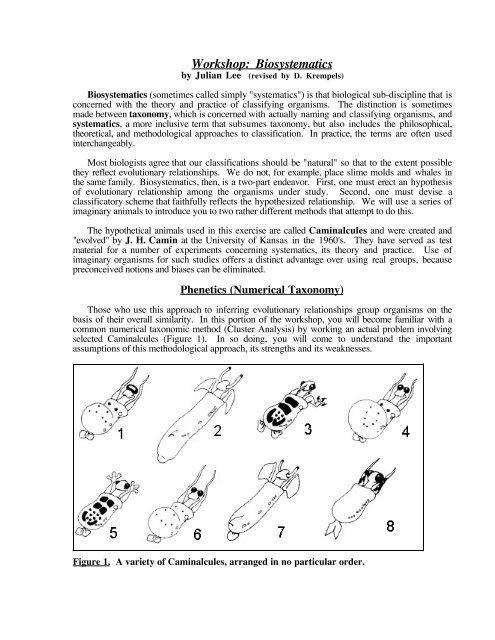
selected Caminalcules (Figure 1). In so doing, you will come to understand the important
assumptions of this methodological approach, its strengths and its weaknesses.
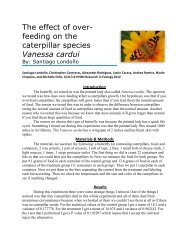
Figure 1. A variety of Caminalcules, arranged in no particular order.

A Sample Procedure
Carefully examine the eight Caminalcules illustrated in Figure 1. These will be your
Operational Taxonomic Units (OTUs)--a name we use to avoid assigning them to any particular
taxonomic rank (such as species). You may think of them as biological species, and refer to them
by number.
The first step is to make a subjective judgement about the overall similarity between all pair-wise
combinations of the eight OTUs, using a scale of 1.0 (maximum similarity) to 0 (complete
disimilarity). These similarity rankings are then cast into a similarity matrix. An example of such a
matrix (for the 8 OTUs in Figure 1) is shown in Table 1.
Table 1. An example of similarity rankings among the eight Caminalcules pictured in
Figure 1. The rankings have been subjectively assigned.
1 2 3 4 5 6 7 8
1 -
2 0.1 -
3 0.2 0.1 -
4 0.7 0.3 0.4 -
5 0.5 0.2 0.8 0.3 -
6 0.8 0.2 0.4 0.7 0.4 -
7 0.1 0.9* 0.2 0.3 0.2 0.3 -
8 0.5 0.3 0.6 0.4 0.6 0.4 0.4 -
Step 1. Find the pair of OTUs that have the highest similarity ranking. (In this example, it happens
to be OTUs 2 and 7, with a similarity ranking of 0.9 shown in boldface and with an asterisk*).
Step 2. Combine OTUs 2 and 7, and treat them as a single composite unit from this point on.
Construct a new similarity matrix (this time it will be 7 x 7), as shown in Table 2.
Table 2. Reduced matrix with similarity values recomputed for all OTUs with composite
OTU 2/7.
2/7 1 3 4 5 6 8
2/7 -
1 0.1 -
3 0.15 0.2 -
4 0.3 0.7 0.4 -
5 0.2 0.5 0.8* 0.3 -
6 0.25 0.8* 0.4 0.7 0.4 -
8 0.35 0.5 0.6 0.4 0.6 0.4 -
Step 3. Recalculate the similarity values for each OTU with the new composite 2/7 OTU. To do
so, simply compute the average similarity of each OTU with 2 and with 7 (listed in Table 1).
In our example, the similarity of OTU 4 with OTU 2 is 0.3, and the similarity of OTU 4 with
OTU 7 is 0.3, then the similarity of OTU 4 with OTU 2/7 will be the average of those two
similarities: [(0.3 + 0.3)/2], or 0.3. The recalculated similarities for each OTU with composite
OTU 2/7 are shown in boldface in Table 2. The new highest similarity value(s) is/are marked with
an asterisk*.
Step 4. In the new, reduced matrix with recomputed similarity values, find the next pair of OTUs
with the highest similarity value. In this case, OTUs 1 and 6 and OTUs 3 and 5 are tied with a
similarity value of 0.8. For simplicity, choose one pairing at random and recalculate the similarity
indices, and then do the next pairing, as shown in Table 3(a).

Table 3. Reduced matrices with similarity values recomputed for all OTUs with (a) new
composite OTU 1/6, (b) new composite OTU 3/5, (c) new composite OTU 4/1/6, and (d)
new composite OTU 8/3/5 and (e) 4/1/6/8/3/5. Again, recalculated similarity indices are
shown in boldface, and the new highest similarity index in each matrix is marked with an
asterisk.
a:
1/6 2/7 3 4 5 8
1/6 -
2/7 0.18 -
3 0.3 0.15 -
4 0.7 0.3 0.4 -
5 0.45 0.2 0.8* 0.3 -
8 0.45 0.35 0.6 0.4 0.6 -
b:
3/5 1/6 2/7 4 8
3/5 -
1/6 0.38 -
2/7 0.35 0.18 -
4 0.35 0.7* 0.3 -
8 0.6 0.45 0.35 0.4 -
c:
4/1/6 3/5 2/7 8
4/1/6 -
3/5 0.37 -
2/7 0.24 0.35 -
8 0.43 0.6* 0.35 -
d:
8/3/5 4/1/6 2/7
8/3/5 -
4/1/6 0.4* -
2/7 0.35 0.24 -
e:
4/1/6/8/3/5 2/7
4/1/6/8/3/5 -
2/7 0.3* -
Step 5. Continue to construct reduced matrices, each time recalculating the similarity indices
between your new composite OTU with all remaining OTUs, as shown in Table 3(b - e). The last
step will result in a 2 x 2 matrix with a single, final similarity value. (In this example, composite
OTY 4/1/6/8/3/5 has a 0.3 similarity to composite OTU 2/7).
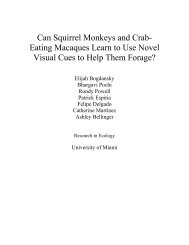
Step 7. Your OTUs can now be clustered graphically in a branching diagram called a phenogram.
The result of our sample cluster analysis is shown in Figure 2. Note that the most similar OTUs
from the first table (OTUs 2 and 7) have been paired at a branch point reflecting their similarity
index (0.9). The next most similar OTU pairings (1/6 and 3/5) have been clustered at their
respective levels (0.8) in the same fashion, and each successive reduced matrix yields the
appropriate branch level, shown on the similarity scale at the left side of the diagram.
This phenogram is designed to not only indicate which of the Caminalcules are supposedly
most physically similar, but also to what degree they are phenotypically similar.

Figure 2. Phenogram of Caminalcules clustered in the sample exercise.
Note again that the similarity values assigned in the example were subjective. Different relative
similarities might have been assigned by a different observer. A phenogram provides a visual
representation of similarity relationships of OTUs, and nothing more. Note that clusters can be
rotated around their branches without changing the implied similarity relationships. For example, if
the diagram were rotated at the 0.3 branch point so that OTUs 2 and 7 were on the right, and OTUs
1, 3, 4, 5, 6 and 8 on the left, the information in the diagram would not be changed. The same would
be true of rotation at any branch point.
Given the computational tedium of working through this simple 8 OTU example, you can see
why real numerical taxonomic studies, which often involve large numbers of OTUs, require the use
of computers.

Exercise
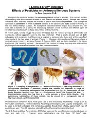
You will now do your own phenogram using a somewhat different group of Caminalcules as
your OTUs. A series of tables is provided below for you to do your reduction calculations, and the
space on the following page is provided so that you may draw a phenogram for your Caminalcules,
shown in Figure 3. Once you have finished the exercise, discuss the questions following the
exercise.
Figure 3. A second set of Caminalcules, arranged in no particular order for you to use in
your own phenetic analysis (and later, in a cladistic analysis).
Questions
1. In the early years of numerical taxonomy, advocates of teh approach claimed that the
methodology would bring objectivity to systematics by the appliation of highly quantitative
techniques, specific algorithms for clustering, and numerical assessment of similarity. What to
make of these claims of objectivity
2. An underlying assumption of numerical taxonomy is that overall similarity is a reliable indicator
of evolutionary relationships (i.e., recency of common ancestry) among organisms. Is this a
reasonable assumption
3. If numerical taxonomy is such a flawed method for inferring evolutoinary relationships, why are
we torturing you with all this (Actually, this is a serious question: Do you believe that cluster
analysis might be of use in other areas of biology If so, in what fields, and how)

Matrices for you to use:
A B C D E F G H
A -
B -
C -
D -
E -
F -
G -
H -

Cladistics (Quantitative Phyletics)
A more objective and suitable method for inferring evoluitionary relationships is cladistics,
sometimes called quantitative phyletics. Rather than grouping OTUs together on the basis of
overall similarity, as in numerical taxonomy, the investigator using this method groups OTUs
together on the basis of shared, derived characters--characters whose presence or absence in two or
more OTUs is inferred to be the result of inheritance form their common ancestor. Thus, in the
branching diagram shown in Figure 4, OTUs A and B are considered most closely related if they
share characters in common not found in OTU C. OTU C is considered most closely related to A
and B if it shares characters common to all three OTUs, but absent from other OTUs outside this
three-OTU grouping. Results of a cladisitc analysis are normally summarized as a branching
diagram called a cladogram (from the Greek clad meaning "branch") (Figure 4), which is an
explicit hypothesis of evolutionary relationships.
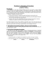
In the cladogram shown, A and B are
considered most closely related if they
share characters in common that are not
found in C. C is considered most closely
related to A and B if it shared charactrers
common to all three OTUs, but absent from
other OTUs outside this three-OTU group.
The cladogram is an explicit hypothesis of
evolutionary relationship.
A taxonomic group descended from a
single common ancestor is said to be
monophyletic if it includes all the
descendants of that common ancestor, and
none of the taxa descended from a different
common ancestor. For example, A and B
would comprise a monophyletic group, but
A and C would not.
Figure 4. A cladogram
A Sample Procedure
We will examine the eight Caminalcules in Figure 1, this time in an attempt to infer the
evolutionary relationships among them, as follows.
Step One. Select a series of characters that can be expressed as binary (i.e., two-state). For
example:
Character a: "eyes present" (+) versus "eyes absent" (-)
Character b: "body mantle present" (+) versus "body mantle absent" (-)
Character c: "paired, anterior tentacles present" (+) versus
"paired, anterior tentacles not present" (-)
Character d: "anterior tentacles flipperlike" (+) versus
"anterior tentacles not flipperlike" (-)
Character e: "eyes stalked" (+) versus "eyes not stalked" (-)
Character f: "body mantle posterior bulbous" (+) versus
"body mantle posterior not bulbous" (-)
Character g: "eyes fused into one" (+) versus "eyes separate" (-)
Character h. "forelimbs with digits" (+) versus "forelimbs without digits" (-)
Step Two. Examine all your organisms and determine which character state it exhibits. Enter the
data in a matrix like the one shown in Table 4.

Table 4. Character states of characters a - h in Caminalcules in Figure 1.
character 1 2 3 4 5 6 7 8
a + + + + + + + +
b + + + + + + + +
c - + - - - - + -
d + + - + - + + +
e - + - - - - + -
f + - - + - + - -
g + - - - - - - -
h - - + - + - - -
Note that in this example, character a (presence or absence of eyes) and character b (presence or
absence of a body mantle) is the same in all eight OTUs. Hence, this (primitive) character is not
useful to us if we are trying to determine differences between the OTUs. (A similar example would
be "hair" in mammals. Since all mammals have hair, the presence of hair in any particular mammal
gives no information about its relationship to other mammals.)
Note also that only OTUs 2 and 7 share character e (stalked eyes), which is absent from all
other OTUs. This suggests that OTUs 2 and 7 both inherited this character from a common
ancestor. Likewise, OTUs 1, 4, and 6 share character f (bulbous mantle posterior) which is absent
from all others. This supports the hypothesis of common ancestry among these three OTUs.. The
same reasoning argues for common ancestry among OTUs 1, 4, and 6 (character f), and for OTUs
3 and 5 (character h), and so on.
A cladogram consistent with the distribution of these eight characters among the eight OTUs is
shown in Figure 5.
Figure 5. A cladogram based on shared, derived characters in Caminalcules 1 - 8.

It is important to note that this is not the only possible branching sequence consistent with the
distribution of the characters among the OTUs. In practice, there are often several, or even many,
cladograms that can be constructed, all of which are consistent with the data. In such cases,
systematists generally apply a parsimony citerion for selecting the "best" cladogram. The rule of
parsimony states that when two or more competing hypotheses are equally consistent with the data,
we provisionally accpet the simplest hypothesis. This is not to say that evolution is always
parsimonious, only that our hypotheses should be.
In the case of competing cladograms, the rule of parsimony would require that we accept the
simplest cladogram--the one with the fewest "steps" to each of the taxa on the tree--is preferred over
a cladogram requiring more evolutionary steps. In our example, we could hypothesize that OTU 6
is actually more closely related to OTU 1 than to OTU 4. However, this would require that
character g (fused eyes) had been evolved once, and then secondarily lost in both OTUs 4 and 6.
This is a less parsimonious hypothesis than one stating fused eyes evolved only once, in OTU 1.
Classification
Given an hypothesis of evolutionary relationships, the second step in biosystematic endeavor is
to erect a classification that faithfully reflects those relationships. Because the results of a cladistic
analysis (i.e., the cladogram) are heirarchical, they can easily be incorporated into the Linnaean
hierarchy, as follows.
Order Caminalcula:
Family 1
Genus 1
Species 2
Species 7
Genus 2
Species 1
Species 4
Species 6
Species 8
Family 2
Genus 1
Species 3
Species 5
In cladistic analysis, all taxa must be monophyletic, meaning that they must include the
common ancestor (almost always hypothetical) and all descendants of that common ancestor. Thus,
in the cladogram above, OTUs 2 and 7 together with their common ancestor (at the branch point
just below them) constitute a monophyletic genus, as do OTUs 1,4,6 and 8 and their common
ancestor (at the branch point just above the appearance of character d).
A Family consisting of only OTUs 2 and 7 would not be monophyletic, because it does not
include all the descendants of the common ancestor (at the branch point just below character d).
Such a group would be considered paraphyletic (containing some, but not all, of a particular
ancestor's descendants).
A Family consisting of OTUs 2 and 7 plus OTUs 3 and 5 would be considered polyphyletic
(consisting of species derived from more than one most recent common ancestor). This is because
such a taxon would be made up of groups descended from both the ancestor just below the
appearance of character h, and the one just below the appearance of characters c and e.
Exercise
Using the Caminalcules in Figure 3, go through the steps of cladistic analysis we just did for
the ones in Figure 1. Use the spaces and matrix provided to choose shared, derived characters that
help you link some of the OTUs in taxa that reflect their hypothetical evolutionary relationships.
Finally, in the space provided, draw a cladogram of your Caminalcules, showing the appearance of
each character as we did in our example.

character state of character if (+) state of character if (-)
a
b
c
d
e
f
g
h
OTUs
character 1 2 3 4 5 6 7 8
a
b
c
d
e
f
g
h
Your cladogram:
Questions
1. The results of phenetic and cladistic analysies are inherently hierarchical, as is the branching
sequence of the evolution of organisms. So, too, is the Linnaean classificatory system of ever more
inclusive taxonomic categories from species, Genus, Family, Order, Class, Phylum, Kingdom and
Domain. Can you name some other hierarchical classification systems (not necessarily biological)
2. Taxonomists were erecting classifications of organisms long before Darwin convinced
biologists of the reality of evolution. Some of these taxonomists believed in the fixity of species
and in special creation. Nevertheless, in some respects, these pre-Darwinian classifications are
rather similar to those produced later by evolutionary taxonomists. Why do you think this is so