From Efficient Markets Theory to Behavioral Finance

Robert J. Shiller 85
share (or of a portfolio of shares representing an index) equals the mathematical
expectation, conditional on all information available at the time, of the present
value P* t of actual subsequent dividends accruing to that share (or portfolio of
shares). P* t is not known at time t and has to be forecasted. Efficient markets say that
price equals the optimal forecast of it.
Different forms of the efficient markets model differ in the choice of the
discount rate in the present value, but the general efficient markets model can be
written just as P t E t P* t , where E t refers to mathematical expectation conditional
on public information available at time t. This equation asserts that any surprising
movements in the stock market must have at their origin some new information
about the fundamental value P* t .
It follows from the efficient markets model that P* t P t U t , where U t is a
forecast error. The forecast error U t must be uncorrelated with any information
variable available at time t, otherwise the forecast would not be optimal; it would
not be taking into account all information. Since the price P t itself is information
at time t, P t and U t must be uncorrelated with each other. Since the variance of the
sum of two uncorrelated variables is the sum of their variances, it follows that the
variance of P* t must equal the variance of P t plus the variance of U t , and hence,
since the variance of U t cannot be negative, that the variance of P* t must be greater
than or equal to that of P t .
Thus, the fundamental principle of optimal forecasting is that the forecast
must be less variable than the variable forecasted. Any forecaster whose forecast
consistently varies through time more than the variable forecasted is making a
serious error, because then high forecasts would themselves tend to indicate
forecast positive errors, and low forecasts indicate negative errors. The maximum
possible variance of the forecast is the variance of the variable forecasted, and this
can occur only if the forecaster has perfect foresight and the forecasts correlate
perfectly with the variable forecasted.
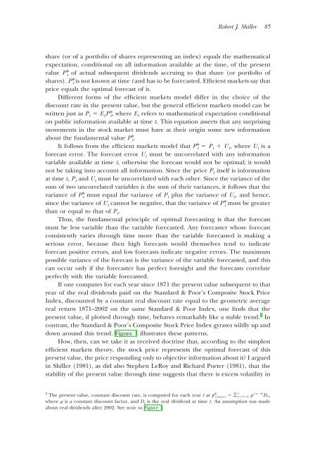
If one computes for each year since 1871 the present value subsequent to that
year of the real dividends paid on the Standard & Poor’s Composite Stock Price
Index, discounted by a constant real discount rate equal to the geometric average
real return 1871–2002 on the same Standard & Poor Index, one finds that the
present value, if plotted through time, behaves remarkably like a stable trend. 2 In
contrast, the Standard & Poor’s Composite Stock Price Index gyrates wildly up and
down around this trend. Figure 1 illustrates these patterns.
How, then, can we take it as received doctrine that, according to the simplest
efficient markets theory, the stock price represents the optimal forecast of this
present value, the price responding only to objective information about it I argued
in Shiller (1981), as did also Stephen LeRoy and Richard Porter (1981), that the
stability of the present value through time suggests that there is excess volatility in
2
The present value, constant discount rate, is computed for each year t as p* const,t ¥ t1 (t) D ,
where is a constant discount factor, and D t is the real dividend at time t. An assumption was made
about real dividends after 2002. See note to Figure 1.