Chapter 5 Discrete Distributions

Chapter 5
Discrete Distributions
In this chapter we introduce discrete random variables, those who take values in a finite or
countably infinite support set. We discuss probability mass functions and some special expectations,
namely, the mean, variance and standard deviation. Some of the more important
discrete distributions are explored in detail, and the more general concept of expectation is
defined, which paves the way for moment generating functions.
We give special attention to the empirical distribution since it plays such a fundamental
role with respect to re sampling and Chapter 13;itwillalsobeneededinSection10.5.1 where
we discuss the Kolmogorov-Smirnov test. Following this is a section in which we introduce a
catalogue of discrete random variables that can be used to model experiments.
There are some comments on simulation, and we mention transformations of random variables
in the discrete case. The interested reader who would like to learn more about any of
the assorted discrete distributions mentioned here should take a look at Univariate Discrete
Distributions by Johnson et al [50].
What do I want them to know
• how to choose a reasonable discrete model under a variety of physical circumstances
• the notion of mathematical expectation, how to calculate it,andbasicproperties
• moment generating functions (yes, I want them to hear about those)
• the general tools of the trade for manipulation of continuous randomvariables,integration,
etc.
• some details on a couple of discrete models, and exposure to a bunch of other ones
• how to make new discrete random variables from old ones
5.1 Discrete Random Variables
As in Chapter 4, all occurrences
5.1.1 Probability Mass Functions
of "support" should be "range"
Discrete random variables are characterized by their supports which take the form
S X = {u 1 , u 2 ,...,u k } or S X = {u 1 , u 2 , u 3 ...}. (5.1.1)
107

108 CHAPTER 5. DISCRETE DISTRIBUTIONS
Every discrete random variable X has associated with it a probability mass function (PMF)
f X : S X → [0, 1] defined by
f X (x) = IP(X = x), x ∈ S X . (5.1.2)
Since values of the PMF represent probabilities, we know from Chapter4 that PMFs enjoy
certain properties. In particular, all PMFs satisfy
1. f X (x) > 0forx ∈ S ,
2. ∑ x∈S f X (x) = 1, and
> should be >= and S should be S_X
3. IP(X ∈ A) = ∑ x∈A f X (x), for any event A ⊂ S .
Delete text from "for" on
Example 5.1. Toss a coin 3 times. The sample space would be
S = {HHH, HTH, THH, TTH, HHT, HTT, THT, TTT} .
Now let X be the number of Heads observed. Then X has support S X = {0, 1, 2, 3}. Assuming
that the coin is fair and was tossed in exactly the same way each time,itisnotunreasonable
to suppose that the outcomes in the sample space are all equally likely. What is the PMF of
X NoticethatX is zero exactly when the outcome TTT occurs, and this event has probability
1/8. Therefore, f X (0) = 1/8, and the same reasoning shows that f X (3) = 1/8. Exactly three
outcomes result in X = 1, thus, f X (1) = 3/8 and f X (3) holds the remaining 3/8probability(the
total is 1). We can represent the PMF with a table:
x ∈ S X 0 1 2 3 Total
f X (x) = IP(X = x) 1/8 3/8 3/8 1/8 1
5.1.2 Mean, Variance, and Standard Deviation
There are numbers associated with PMFs. One important example is the mean µ, alsoknown
as IE X:
∑
µ = IE X = xf X (x), (5.1.3)
provided the (potentially infinite) series ∑ |x| f X (x)isconvergent.Anotherimportantnumberis
the variance:
∑
σ 2 = IE(X − µ) 2 = (x − µ) 2 f X (x), (5.1.4)
which can be computed (see Exercise 5.4) withthealternateformulaσ 2 = IE X 2 − (IE X) 2 .
Directly defined from the variance is the standard deviation σ = √ σ 2 .
Example 5.2. We will calculate the mean of X in Example 5.1.
3.5 should be 1.5
3∑
µ = xf X (x) = 0 · 1
8 + 1 · 3
8 + 2 · 3
8 + 3 · 1
8 = 3.5.
x=0
We interpret µ = 3.5byreasoningthatifweweretorepeattherandomexperimentmany times,
independently each time, observe many corresponding outcomes of the random variable X,and
take the sample mean of the observations, then the calculatedvaluewouldfallcloseto3.5.The
approximation would get better as we observe more and more values of X (another form of the
Law of Large Numbers; see Section 4.3). Another way it is commonly stated is that X is 3.5
“on the average” or “in the long run”.
x∈S
x∈S

5.1. DISCRETE RANDOM VARIABLES 109
Remark 5.3. Note that although we say X is 3.5 on the average, we must keep in mind that our
X never actually equals 3.5 (in fact, it is impossible for X to equal 3.5).
Related to the probability mass function f X (x) = IP(X = x) isanotherimportantfunction
called the cumulative distribution function (CDF), F X .Itisdefinedbytheformula
F X (t) = IP(X ≤ t), −∞ < t < ∞. (5.1.5)
We know that all PMFs satisfy certain properties, and a similar statement may be made for
CDFs. In particular, any CDF F X satisfies
• F X is nondecreasing (t 1 ≤ t 2 implies F X (t 1 ) ≤ F X (t 2 )).
• F X is right-continuous (lim t→a + F X (t) = F X (a)foralla ∈ R).
• lim t→−∞ F X (t) = 0andlim t→∞ F X (t) = 1.
We say that X has the distribution F X and we write X ∼ F X .Inanabuseofnotationwewill
also write X ∼ f X and for the named distributions the PMF or CDF will be identified by the
family name instead of the defining formula. Actually, the ~ notation is
standard only for distributions
specified by name and parameters
5.1.3 How to do it with R
The mean and variance of a discrete random variable is easy to compute at the console. Let’s
return to Example 5.2. Wewillstartbydefiningavectorx containing the support of X, anda
vector f to contain the values of f X at the respective outcomes in x:
> x f mu mu
[1] 1.5
To compute the variance σ 2 ,wesubtractthevalueofmu from each entry in x, squarethe
answers, multiply by f, andsum. Thestandarddeviationσ is simply the square root of σ 2 .
> sigma2 sigma2
[1] 0.75
> sigma sigma
[1] 0.8660254
Finally, we may find the values of the CDF F X on the support by accumulating the probabilities
in f X with the cumsum function.

110 CHAPTER 5. DISCRETE DISTRIBUTIONS
> F = cumsum(f)
> F
[1] 0.125 0.500 0.875 1.000
As easy as this is, it is even easier to do with the distrEx package [74]. We define a
random variable X as an object, then compute things from the object such as mean, variance,
and standard deviation with the functions E, var, andsd:
> library(distrEx)
> X E(X); var(X); sd(X)
[1] 1.5
[1] 0.75
[1] 0.8660254
5.2 The Discrete Uniform Distribution
We have seen the basic building blocks of discrete distributions and we now study particular
models that statisticians often encounter in the field. Perhaps the most fundamental of all is the
discrete uniform distribution.
ArandomvariableX with the discrete uniform distribution on the integers 1, 2,...,m has
PMF
f X (x) = 1 , x = 1, 2,...,m. (5.2.1)
m
We write X ∼ disunif(m). A random experiment where this distribution occurs is the choice
of an integer at random between 1 and 100, inclusive. Let X be the number chosen. Then
X ∼ disunif(m = 100) and
IP(X = x) = 1
100 , x = 1,...,100.
We find a direct formula for the mean of X ∼ disunif(m):
m∑
m∑
µ = xf X (x) = x · 1
m = 1 m + 1
(1 + 2 + ···+ m) =
m 2 , (5.2.2)
x=1
x=1
where we have used the famous identity 1 + 2 + ···+ m = m(m + 1)/2. That is, if we repeatedly
choose integers at random from 1 to m then, on the average, we expect to get (m + 1)/2. To get
the variance we first calculate
and finally,
IE X 2 = 1 m
m∑
x=1
σ 2 = IE X 2 − (IE X) 2 =
x 2 = 1 m(m + 1)(2m + 3)
=
m 6
(m + 1)(2m + 1)
6
( m + 1
−
2
(m + 1)(2m + 1)
,
6
) 2
= ···= m2 − 1
12 . (5.2.3)
Example 5.4. Roll a die and let X be the upward face showing. Then m = 6, µ = 7/2 = 3.5,
and σ 2 = (6 2 − 1)/12 = 35/12.

5.3. THE BINOMIAL DISTRIBUTION 111
5.2.1 How to do it with R
From the console: One can choose an integer at random with the sample function. The general
syntax to simulate a discrete uniform random variable is sample(x, size, replace
= TRUE).
The argument x identifies the numbers from which to randomly sample. If x is a number,
then sampling is done from 1 to x. Theargumentsize tells how big the sample size should
be, and replace tells whether or not numbers should be replaced in the urn after having been
sampled. The default option is replace = FALSE but for discrete uniforms the sampled values
should be replaced. Some examples follow.
5.2.2 Examples
• To roll a fair die 3000 times, do sample(6, size = 3000, replace = TRUE).
• To choose 27 random numbers from 30 to 70, do sample(30:70, size = 27, replace
= TRUE).
• To flip a fair coin 1000 times, do sample(c("H","T"), size = 1000, replace =
TRUE).
With the R Commander: Follow the sequence Probability ⊲ Discrete Distributions ⊲ Discrete
Uniform distribution ⊲ Simulate Discrete uniform variates. . . .
Suppose we would like to roll a fair die 3000 times. In the Number of samples field we
enter 1. Next,wedescribewhatintervalofintegerstobesampled.Since there are six faces
numbered 1 through 6, we set from = 1, wesetto = 6, andsetby = 1 (to indicate that we
travel from 1 to 6 in increments of 1 unit). We will generate a list of 3000 numbers selected
from among 1, 2, . . . , 6, and we store the results of the simulation. For the time being, we
select New Data set. ClickOK.
Since we are defining a new data set, the R Commander requests a name for the data set. The
default name is Simset1,althoughinprincipleyoucouldnameitwhateveryoulike(according
to R’s rules for object names). We wish to have a list that is 3000 long, so we set Sample
Size = 3000 and click OK.
In the R Console window, the R Commander should tell you that Simset1 has been initialized,
and it should also alert you that There was 1 discrete uniform variate sample
stored in Simset 1.. Totakealookattherollsofthedie,weclickView data set and a
window opens.
The default name for the variable is disunif.sim1.
5.3 The Binomial Distribution
The binomial distribution is based on a Bernoulli trial,whichisarandomexperimentinwhich
there are only two possible outcomes: success (S )andfailure(F). We conduct the Bernoulli
trial and let
⎧
⎪⎨ 1 iftheoutcomeis S ,
X =
(5.3.1)
⎪⎩ 0 iftheoutcomeis F.

112 CHAPTER 5. DISCRETE DISTRIBUTIONS
If the probability of success is p then the probability of failure must be 1 − p = q and the PMF
of X is
f X (x) = p x (1 − p) 1−x , x = 0, 1. (5.3.2)
It is easy to calculate µ = IE X = p and IE X 2 = p so that σ 2 = p − p 2 = p(1 − p).
5.3.1 The Binomial Model
The Binomial model has three defining properties:
• Bernoulli trials are conducted n times,
• the trials are independent,
• the probability of success p does not change between trials.
If X counts the number of successes in the n independent trials, then the PMF of X is
( n
f X (x) = p
x)
x (1 − p) n−x , x = 0, 1, 2,...,n. (5.3.3)
We say that X has a binomial distribution and we write X ∼ binom(size = n, prob = p). It
is clear that f X (x) ≥ 0forallx in the support because the value is the product of nonnegative
numbers. We next check that ∑ f (x) = 1:
We next find the mean:
n∑
x=0
( n
x)
p x (1 − p) n−x = [p + (1 − p)] n = 1 n = 1.
µ =
n∑
x=0
( n
x p
x)
x (1 − p) n−x ,
n∑ n!
= x
x!(n − x)! px q n−x ,
x=1
n∑ (n − 1)!
=n · p
(x − 1)!(n − x)! px−1 q n−x ,
x=1
∑n−1
( ) n − 1
=np
p (x−1) (1 − p) (n−1)−(x−1) ,
x − 1
=np.
x−1=0
AsimilarargumentshowsthatIEX(X − 1) = n(n − 1)p 2 (see Exercise 5.5). Therefore
σ 2 = IE X(X − 1) + IE X − [IE X] 2 ,
=n(n − 1)p 2 + np − (np) 2 ,
=n 2 p 2 − np 2 + np − n 2 p 2 ,
=np − np 2 = np(1 − p).

5.3. THE BINOMIAL DISTRIBUTION 113
Example 5.5. Afour-childfamily.Eachchildmaybeeitheraboy(B) oragirl(G). For simplicity
we suppose that IP(B) = IP(G) = 1/2andthatthegendersofthechildrenaredetermined
independently. If we let X count the number of B’s, then X ∼ binom(size = 4, prob = 1/2).
Further, IP(X = 2) is
( 4
f X (2) = (1/2)
2)
2 (1/2) 2 = 6 2 . 4
The mean number of boys is 4(1/2) = 2andthevarianceofX is 4(1/2)(1/2) = 1.
5.3.2 How to do it with R
The corresponding R function for the PMF and CDF are dbinom and pbinom,respectively.We
demonstrate their use in the following examples.
Example 5.6. We can calculate it in R Commander under the Binomial Distribution menu with
the Binomial probabilities menu item.
Pr
0 0.0625
1 0.2500
2 0.3750
3 0.2500
4 0.0625
We know that the binom(size = 4, prob = 1/2) distribution is supported on the integers 0,
1, 2, 3, and 4; thus the table is complete. We can read off the answer to be IP(X = 2) = 0.3750.
Example 5.7. Roll 12 dice simultaneously, and let X denote the number of 6’s that appear. We
wish to find the probability of getting seven, eight, or nine 6’s. If we let S = { get a 6 on one roll } ,
then IP(S ) = 1/6andtherollsconstituteBernoullitrials;thusX ∼ binom(size =12, prob =1/6)
and our task is to find IP(7 ≤ X ≤ 9). This is just
IP(7 ≤ X ≤ 9) =
9∑ ( 12
x
x=7
)
(1/6) x (5/6) 12−x .
Again, one method to solve this problem would be to generate a probability mass table and add
up the relevant rows. However, an alternative method is to notice that IP(7 ≤ X ≤ 9) = IP(X ≤
9) − IP(X ≤ 6) = F X (9) − F X (6), so we could get the same answer by using the Binomial tail
probabilities. . . menu in the R Commander or the following from the command line:
> pbinom(9, size=12, prob=1/6) - pbinom(6, size=12, prob=1/6)
[1] 0.001291758
> diff(pbinom(c(6,9), size = 12, prob = 1/6)) # same thing
[1] 0.001291758

114 CHAPTER 5. DISCRETE DISTRIBUTIONS
Example 5.8. Toss a coin three times and let X be the number of Heads observed. We know
from before that X ∼ binom(size = 3, prob = 1/2) which implies the following PMF:
x = #of Heads 0 1 2 3
f (x) = IP(X = x) 1/8 3/8 3/8 1/8
Our next goal is to write down the CDF of X explicitly. The first case is easy: it is impossible
for X to be negative, so if x < 0thenweshouldhaveIP(X ≤ x) = 0. Now choose a value x
satisfying 0 ≤ x < 1, say, x = 0.3. The only way that X ≤ x could happen would be if X = 0,
therefore, IP(X ≤ x) shouldequalIP(X = 0), and the same is true for any 0 ≤ x < 1. Similarly,
for any 1 ≤ x < 2, say, x = 1.73, the event {X ≤ x} is exactly the event {X = 0orX = 1}.
Consequently, IP(X ≤ x)shouldequalIP(X = 0orX = 1) = IP(X = 0) + IP(X = 1). Continuing
in this fashion, we may figure out the values of F X (x) forallpossibleinputs−∞ < x < ∞, and
we may summarize our observations with the following piecewise defined function:
⎧
0, x < 0,
1
⎪⎨
, 0 ≤ x < 1,
8
1
F X (x) = IP(X ≤ x) = + 3 = 4, 1 ≤ x < 2,
8 8 8
4
8
⎪⎩
+ 3 = 7, 2 ≤ x < 3,
8 8
1, x ≥ 3.
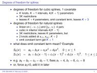
In particular, the CDF of X is defined for the entire real line, R. TheCDFisrightcontinuous
and nondecreasing. A graph of the binom(size = 3, prob = 1/2) CDF is shown in Figure
5.3.1.
Example 5.9. Another way to do Example 5.8 is with the distr family of packages [74]. They
use an object oriented approach to random variables, that is, arandomvariableisstoredinan
object X, andthenquestionsabouttherandomvariabletranslatetofunctions on and involving
X. Randomvariableswithdistributionsfromthebase package are specified by capitalizing the
name of the distribution.
> library(distr)
> X X
Distribution Object of Class: Binom
size: 3
prob: 0.5
The analogue of the dbinom function for X is the d(X) function, and the analogue of the
pbinom function is the p(X) function. Compare the following:
> d(X)(1) # pmf of X evaluated at x = 1
[1] 0.375
> p(X)(2) # cdf of X evaluated at x = 2
[1] 0.875

5.3. THE BINOMIAL DISTRIBUTION 115
cumulative probability
0.0 0.2 0.4 0.6 0.8 1.0
−1 0 1 2 3 4
number of successes
Figure 5.3.1: Graph of the binom(size = 3, prob = 1/2) CDF
Random variables defined via the distr package may be plotted,whichwillreturngraphs
of the PMF, CDF, and quantile function (introduced in Section 6.3.1). See Figure 5.3.2 for an
example.

116 CHAPTER 5. DISCRETE DISTRIBUTIONS
Given X ∼ dbinom(size = n, prob = p).
How to do: with stats (default) with distr
PMF: IP(X = x) dbinom(x, size = n, prob = p) d(X)(x)
CDF: IP(X ≤ x) pbinom(x, size = n, prob = p) p(X)(x)
Simulate k variates rbinom(k, size = n, prob = p) r(X)(k)
For distr need X

5.4. EXPECTATION AND MOMENT GENERATING FUNCTIONS 117
Definition 5.10. More generally, given a function g we define the expected value of g(X) by
This should be a theorem, ∑
not a definition IE g(X) = g(x) f X (x), (5.4.2)
x∈S
provided the (potentially infinite) series ∑ x |g(x)| f (x)isconvergent.WesaythatIEg(X) exists.
In this notation the variance is σ 2 = IE(X − µ) 2 and we prove the identity
IE(X − µ) 2 = IE X 2 − (IE X) 2 (5.4.3)
in Exercise 5.4. Intuitively,forrepeatedobservationsofX we would expect the sample mean
of the g(X)valuestocloselyapproximateIEg(X) asthesamplesizeincreaseswithoutbound.
Let us take the analogy further. If we expect g(X) tobeclosetoIEg(X) ontheaverage,
where would we expect 3g(X) tobeontheaverageItcouldonlybe3IEg(X). The following
theorem makes this idea precise.
Proposition 5.11. For any functions g and h, any random variable X, and any constant c:
1. IE c = c,
2. IE[c · g(X)] = c IE g(X)
3. IE[g(X) + h(X)] = IE g(X) + IE h(X),
provided IE g(X) and IE h(X) exist.
Proof. Go directly from the definition. For example,
∑
∑
IE[c · g(X)] = c · g(x) f X (x) = c · g(x) f X (x) = c IE g(X).
x∈S
x∈S
□
5.4.2 Moment Generating Functions
Definition 5.12. Given a random variable X, itsmoment generating function (abbreviated
MGF) is defined by the formula
∑
M X (t) = IE e tX = e tx f X (x), (5.4.4)
provided the (potentially infinite) series is convergent for allt in a neighborhood of zero (that
is, for all −ɛ < t < ɛ, forsomeɛ > 0).
Note that for any MGF M X ,
x∈S
M X (0) = IE e 0·X = IE 1 = 1. (5.4.5)
We will calculate the MGF for the two distributions introduced above.
Example 5.13. Find the MGF for X ∼ disunif(m).
Since f (x) = 1/m, theMGFtakestheform
M(t) =
m∑
e tx 1 m = 1 m (et + e 2t + ···+ e mt ), for any t.
x=1

118 CHAPTER 5. DISCRETE DISTRIBUTIONS
Example 5.14. Find the MGF for X ∼ binom(size = n, prob = p).
Applications
n∑ ( ) n
M X (t) = e tx p x (1 − p) n−x ,
x
x=0
∑n−x
( n
= (pe
x)
t ) x q n−x ,
x=0
=(pe t + q) n , for any t.
We will discuss three applications of moment generating functions in this book. The first is the
fact that an MGF may be used to accurately identify the probability distribution that generated
it, which rests on the following:
Theorem 5.15. The moment generating function, if it exists in a neighborhood of zero, determines
a probability distribution uniquely.
Proof. Unfortunately, the proof of such a theorem is beyond the scope ofatextlikethisone.
Interested readers could consult Billingsley [8].
□
We will see an example of Theorem 5.15 in action.
Example 5.16. Suppose we encounter a random variable which has MGF
Then X ∼ binom(size = 13, prob = 0.7).
M X (t) = (0.3 + 0.7e t ) 13 .
An MGF is also known as a “Laplace Transform” and is manipulated in that context in
many branches of science and engineering.
Why is it called a Moment Generating Function
This brings us to the second powerful application of MGFs. Many of the models we study
have a simple MGF, indeed, which permits us to determine the mean, variance, and even higher
moments very quickly. Let us see why. We already know that
∑
M(t) = e tx f (x).
x∈S
Take the derivative with respect to t to get
M ′ (t) = d ⎛ ⎞
∑ ∑
dt
⎜⎝ e tx f (x) ⎟⎠ =
x∈S
x∈S
d
dt
( e tx f (x) ) ∑
= xe tx f (x), (5.4.6)
and so if we plug in zero for t we see
∑ ∑
M ′ (0) = xe 0 f (x) = xf(x) = µ = IE X. (5.4.7)
x∈S
x∈S
x∈S

5.4. EXPECTATION AND MOMENT GENERATING FUNCTIONS 119
Similarly, M ′′ (t) = ∑ x 2 e tx f (x)sothatM ′′ (0) = IE X 2 .Andingeneral,wecansee 2 that
M (r)
X (0) = IE Xr = r th moment of Xabout the origin. (5.4.8)
These are also known as raw moments and are sometimes denoted µ ′ r.Inadditiontotheseare
the so called central moments µ r defined by
µ r = IE(X − µ) r , r = 1, 2,... (5.4.9)
Example 5.17. Let X ∼ binom(size = n, prob = p)withM(t) = (q + pe t ) n .Wecalculated
the mean and variance of a binomial random variable in Section 5.3 by means of the binomial
series. But look how quickly we find the mean and variance with the moment generating
function.
And
Therefore
See how much easier that was
M ′ (t) =n(q + pe t ) n−1 pe t | t=0 ,
=n · 1 n−1 p,
=np.
M ′′ (0) =n(n − 1)[q + pe t ] n−2 (pe t ) 2 + n[q + pe t ] n−1 pe t | t=0 ,
IE X 2 =n(n − 1)p 2 + np.
σ 2 = IE X 2 − (IE X) 2 ,
=n(n − 1)p 2 + np − n 2 p 2 ,
=np − np 2 = npq.
Remark 5.18. We learned in this section that M (r) (0) = IE X r .WerememberfromCalculusII
that certain functions f can be represented by a Taylor series expansion about a point a, which
takes the form
∞∑ f (r) (a)
f (x) = (x − a) r , for all |x − a| < R, (5.4.10)
r!
r=0
where R is called the radius of convergence of the series (see Appendix E.3). We combine the
two to say that if an MGF exists for all t in the interval (−ɛ, ɛ), then we can write
M X (t) =
∞∑ IE X r
t r , for all |t| < ɛ. (5.4.11)
r!
r=0
2 We are glossing over some significant mathematical details inourderivation.Suffice it to say that when the
MGF exists in a neighborhood of t = 0, the exchange of differentiation and summation is valid in that neighborhood,
and our remarks hold true.

120 CHAPTER 5. DISCRETE DISTRIBUTIONS
5.4.3 How to do it with R
The distrEx package provides an expectation operator E which can be used on random variables
that have been defined in the ordinary distr sense:
> X library(distrEx)
> E(X)
[1] 1.35
> E(3 * X + 4)
[1] 8.05
For discrete random variables with finite support, the expectation is simply computed with
direct summation. In the case that the random variable has infinite support and the function is
crazy, then the expectation is not computed directly, rather, it is estimated by first generating a
random sample from the underlying model and next computing a sample mean of the function
of interest.
There are methods for other population parameters:
> var(X)
[1] 0.7425
> sd(X)
[1] 0.8616844
There are even methods for IQR, mad, skewness,andkurtosis.
5.5 The Empirical Distribution
Do an experiment n times and observe n values x 1 , x 2 ,...,x n of a random variable X. Forsimplicity
in most of the discussion that follows it will be convenient to imagine that the observed
values are distinct, but the remarks are valid even when the observed values are repeated.
Definition 5.19. The empirical cumulative distribution function F n (written ECDF) is the probability
distribution that places probability mass 1/n on each of the values x 1 , x 2 ,...,x n .The
empirical PMF takes the form
f X (x) = 1 n , x ∈ {x 1, x 2 ,...,x n } . (5.5.1)
If the value x i is repeated k times, the mass at x i is accumulated to k/n.
The mean of the empirical distribution is
∑
µ = xf X (x) =
x∈S
n∑
i=1
x i · 1
n
(5.5.2)
and we recognize this last quantity to be the sample mean, x. The variance of the empirical
distribution is
∑
n∑
σ 2 = (x − µ) 2 f X (x) = (x i − x) 2 · 1
(5.5.3)
n
x∈S
i=1

5.5. THE EMPIRICAL DISTRIBUTION 121
and this last quantity looks very close to what we already knowtobethesamplevariance.
s 2 = 1
n − 1
n∑
(x i − x) 2 . (5.5.4)
i=1
The empirical quantile function is the inverse of the ECDF. See Section 6.3.1.
5.5.1 How to do it with R
The empirical distribution is not directly available as a distribution in the same way that the
other base probability distributions are, but there are plenty of resources available for the determined
investigator.
Given a data vector of observed values x, wecanseetheempiricalCDFwiththeecdf
function:
> x ecdf(x)
Empirical CDF
Call: ecdf(x)
x[1:5] = 4, 7, 9, 11, 12
The above shows that the returned value of ecdf(x) is not a number but rather a function.
The ECDF is not usually used by itself in this form, by itself. More commonly it is used as
an intermediate step in a more complicated calculation, for instance, in hypothesis testing (see
Chapter 10)orresampling(seeChapter13). It is nevertheless instructive to see what the ecdf
looks like, and there is a special plot method for ecdf objects.
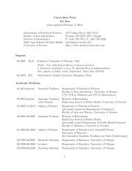
> plot(ecdf(x))

122 CHAPTER 5. DISCRETE DISTRIBUTIONS
ecdf(x)
Fn(x)
0.0 0.2 0.4 0.6 0.8 1.0
2 4 6 8 10 12 14
x
Figure 5.5.1: The empirical CDF
See Figure 5.5.1. The graph is of a right-continuous function with jumps exactly at the
locations stored in x. Therearenorepeatedvaluesinx so all of the jumps are equal to 1/5 =
0.2.
The empirical PDF is not usually of particular interest in itself, but if we really wanted we
could define a function to serve as the empirical PDF:
> epdf x epdf(x)(0) # should be 2/3
[1] 0.6666667
To simulate from the empirical distribution supported on thevectorx, weusethesample
function.
> x sample(x, size = 7, replace = TRUE)
[1] 0 1 0 1 1 0 0
We can get the empirical quantile function in R with quantile(x, probs = p, type
= 1);seeSection6.3.1.
As we hinted above, the empirical distribution is significantmorebecauseofhowandwhere
it appears in more sophisticated applications. We will explore some of these in later chapters –
see, for instance, Chapter 13.

5.6. OTHER DISCRETE DISTRIBUTIONS 123
5.6 Other Discrete Distributions
The binomial and discrete uniform distributions are popular, and rightly so; they are simple and
form the foundation for many other more complicated distributions. But the particular uniform
and binomial models only apply to a limited range of problems. Inthissectionweintroduce
situations for which we need more than what the uniform and binomial offer.
5.6.1 Dependent Bernoulli Trials
The Hypergeometric Distribution
Consider an urn with 7 white balls and 5 black balls. Let our random experiment be to randomly
select 4 balls, without replacement, from the urn. Then the probability of observing 3 white
balls (and thus 1 black ball) would be
( 7
)( 5
3 1)
IP(3W, 1B) = ( 12
) . (5.6.1)
4
More generally, we sample without replacement K times from an urn with M white balls and
N black balls. Let X be the number of white balls in the sample. The PMF of X is
( M
)( N
)
x K−x
f X (x) = ) . (5.6.2)
We say that X has a hypergeometric distribution and write X ∼ hyper(m = M, n = N, k = K).
The support set for the hypergeometric distribution is a little bit tricky. It is tempting to say
that x should go from 0 (no white balls in the sample) to K (no black balls in the sample), but
that does not work if K > M, becauseitisimpossibletohavemorewhiteballsinthesample
than there were white balls originally in the urn. We have the same trouble if K > N. Thegood
news is that the majority of examples we study have K ≤ M and K ≤ N and we will happily
take the support to be x = 0, 1, ...,K.
It is shown in Exercise 5.6 that
µ = K M
M + N , σ2 = K MN M + N − K
(M + N) 2 M + N − 1 . (5.6.3)
The associated R functions for the PMF and CDF are dhyper(x, m, n, k) and phyper,
respectively. There are two more functions: qhyper, whichwewilldiscussinSection6.3.1,
and rhyper,discussedbelow.
Example 5.20. Suppose in a certain shipment of 250 Pentium processors there are17defective
processors. A quality control consultant randomly collects 5 processors for inspection to
determine whether or not they are defective. Let X denote the number of defectives in the
sample.
( M+N
K
1. Find the probability of exactly 3 defectives in the sample,thatis,findIP(X = 3).
Solution: We know that X ∼ hyper(m = 17, n = 233, k = 5). So the required probability
is just
)
To calculate it in R we just type
f X (3) =
( 17
)( 233
3 2
( 250
5
) .

124 CHAPTER 5. DISCRETE DISTRIBUTIONS
> dhyper(3, m = 17, n = 233, k = 5)
[1] 0.002351153
To find it with the R Commander we go Probability ⊲ Discrete Distributions ⊲ Hypergeometric
distribution ⊲ Hypergeometric probabilities....Wefillintheparametersm = 17,
n = 233, and k = 5. Click OK, andthefollowingtableisshowninthewindow.
> A rownames(A) A
Pr
0 7.011261e-01
1 2.602433e-01
2 3.620776e-02
3 2.351153e-03
4 7.093997e-05
We wanted IP(X = 3), and this is found from the table to be approximately 0.0024. The
value is rounded to the fourth decimal place.
We know from our above discussion that the sample space shouldbex = 0, 1, 2, 3, 4, 5,
yet, in the table the probabilities are only displayed for x = 1, 2, 3, and 4. What is
happening As it turns out, the R Commander will only display probabilities that are
0.00005 or greater. Since x = 5isnotshown,itsuggeststhattheoutcomehasatiny
probability. To find its exact value we use the dhyper function:
> dhyper(5, m = 17, n = 233, k = 5)
[1] 7.916049e-07
In other words, IP(X = 5) ≈ 0.0000007916049, a small number indeed.
2. Find the probability that there are at most 2 defectives in the sample, that is, compute
IP(X ≤ 2).
Solution: Since IP(X ≤ 2) = IP(X = 0, 1, 2), one way to do this would be to add the 0,
1, and 2 entries in the above table. this gives 0.7011 + 0.2602 + 0.0362 = 0.9975. Our
answer should be correct up to the accuracy of 4 decimal places. However, a more precise
method is provided by the R Commander. Under the Hypergeometric distribution menu
we select Hypergeometric tail probabilities.. .Wefillintheparametersm, n, andk as
before, but in the Variable value(s) dialog box we enter the value 2. We notice that the
Lower tail option is checked, and we leave that alone. Click OK.
> phyper(2, m = 17, n = 233, k = 5)
[1] 0.9975771
And thus IP(X ≤ 2) ≈ 0.9975771. We have confirmed that the above answer was correct
up to four decimal places.

5.6. OTHER DISCRETE DISTRIBUTIONS 125
3. Find IP(X > 1).
The table did not give us the explicit probability IP(X = 5), so we can not use the table to
give us this probability. We need to use another method. Since IP(X > 1) = 1 − IP(X ≤
1) = 1 − F X (1), we can find the probability with Hypergeometric tail probabilities.. .
We enter 1 for Variable Value(s),weentertheparametersasbefore,andinthiscasewe
choose the Upper tail option. This results in the following output.
> phyper(1, m = 17, n = 233, k = 5, lower.tail = FALSE)
[1] 0.03863065
In general, the Upper tail option of a tail probabilities dialog computes IP(X > x) for
all given Variable Value(s) x.
4. Generate 100, 000 observations of the random variable X.
We can randomly simulate as many observations of X as we want in R Commander.
Simply choose Simulate hypergeometric variates. . . in the Hypergeometric distribution
dialog.
In the Number of samples dialog, type 1. Enter the parameters as above. Under the
Store Values section, make sure New Data set is selected. Click OK.
Anewdialogshouldopen,withthedefaultnameSimset1. Wecouldchangethisifwe
like, according to the rules for R object names. In the sample size box, enter 100000.
Click OK.
In the Console Window, R Commander should issue an alert that Simset1 has been
initialized, and in a few seconds, it should also state that 100,000 hypergeometric variates
were stored in hyper.sim1. We can view the sample by clicking the View Data Set
button on the R Commander interface.
We know from our formulas that µ = K · M/(M + N) = 5 ∗ 17/250 = 0.34. We can check
our formulas using the fact that with repeated observations of X we would expect about
0.34 defectives on the average. To see how our sample reflects the true mean, we can
compute the sample mean
Rcmdr> mean(Simset2$hyper.sim1, na.rm=TRUE)
[1] 0.340344
Rcmdr> sd(Simset2$hyper.sim1, na.rm=TRUE)
[1] 0.5584982
.
We see that when given many independent observations of X, thesamplemeanisvery
close to the true mean µ. We can repeat the same idea and use the sample standard
deviation to estimate the true standard deviation of X. Fromtheoutputaboveourestimate
is 0.5584982, and from our formulas we get
σ 2 = K
MN M + N − K
(M + N) 2 M + N − 1 ≈ 0.3117896,
with σ = √ σ 2 ≈ 0.5583811944. Our estimate was pretty close.
From the console we can generate random hypergeometric variates with the rhyper
function, as demonstrated below.

126 CHAPTER 5. DISCRETE DISTRIBUTIONS
> rhyper(10, m = 17, n = 233, k = 5)
[1] 0 0 0 0 0 2 0 0 0 1
Sampling With and Without Replacement
Suppose that we have a large urn with, say, M white balls and N black balls. We take a sample
of size n from the urn, and let X count the number of white balls in the sample. If we sample
without replacement, then X ∼ hyper(m =M, n = N, k = n)andhasmeanandvariance
On the other hand, if we sample
M
µ =n
M + N ,
σ 2 MN M + N − n
=n
(M + N) 2 M + N − 1 ,
M
(
M
) M + N − n
=n 1 −
M + N M + N M + N − 1 .
with replacement, then X ∼ binom(size = n, prob = M/(M + N)) with mean and variance
M
µ =n
M + N ,
σ 2 M
=n
M + N
(
1 −
M
)
.
M + N
We see that both sampling procedures have the same mean, and the method with the larger
variance is the “with replacement” scheme. The factor by which the variances differ,
M + N − n
M + N − 1 , (5.6.4)
is called a finite population correction. Forafixedsamplesizen, asM, N →∞it is clear that
the correction goes to 1, that is, for infinite populations the samplingschemesareessentially
the same with respect to mean and variance.
5.6.2 Waiting Time Distributions
Another important class of problems is associated with the amount of time it takes for a specified
event of interest to occur. For example, we could flip a coin repeatedly until we observe
Heads. We could toss a piece of paper repeatedly until we make it in the trash can.
The Geometric Distribution
Suppose that we conduct Bernoulli trials repeatedly, noting thesuccessesandfailures. LetX
be the number of failures before a success. If IP(S ) = p then X has PMF
f X (x) = p(1 − p) x , x = 0, 1, 2,... (5.6.5)
(Why) We say that X has a Geometric distribution and we write X ∼ geom(prob = p).
The associated R functions are dgeom(x, prob), pgeom, qgeom, andrhyper, whichgivethe
PMF, CDF, quantile function, and simulate random variates, respectively. rgeom

5.6. OTHER DISCRETE DISTRIBUTIONS 127
Again it is clear that f (x) ≥ 0andwecheckthat ∑ f (x) = 1(seeEquationE.3.9 in Appendix
E.3):
∞∑
∞∑
p(1 − p) x =p q x 1
= p
1 − q = 1.
x=0
We will find in the next section that the mean and variance are
µ = 1 − p
p
x=0
= q p and σ2 = q p 2 . (5.6.6)
Example 5.21. The Pittsburgh Steelers place kicker, Jeff Reed, made 81.2% of his attempted
field goals in his career up to 2006. Assuming that his successive field goal attempts are approximately
Bernoulli trials, find the probability that Jeff misses at least 5 field goals before his
first successful goal.
Solution: IfX = the number of missed goals until Jeff’s first success, then X ∼ geom(prob =
0.812) and we want IP(X ≥ 5) = IP(X > 4). We can find this in R with
> pgeom(4, prob = 0.812, lower.tail = FALSE)
[1] 0.0002348493
Note 5.22. Some books use a slightly different definition of the geometric distribution. They
consider Bernoulli trials and let Y count instead the number of trials until a success, so that Y
has PMF
f Y (y) = p(1 − p) y−1 , y = 1, 2, 3,... (5.6.7)
When they say “geometric distribution”, this is what they mean. It is not hard to see that the
two definitions are related. In fact, if X denotes our geometric and Y theirs, then Y = X + 1.
Consequently, they have µ Y = µ X + 1andσ 2 Y = σ2 X .
The Negative Binomial Distribution
We may generalize the problem and consider the case where we wait for more than one success.
Suppose that we conduct Bernoulli trials repeatedly, noting the respective successes and
failures. Let X count the number of failures before r successes. If IP(S ) = p then X has PMF
( ) r + x − 1
f X (x) = p r (1 − p) x , x = 0, 1, 2,... (5.6.8)
r − 1
We say that X has a Negative Binomial distribution and write X ∼ nbinom(size = r, prob =
p). The associated R functions are dnbinom(x, size, prob), pnbinom, qnbinom, and
rnbinom, whichgivethePMF,CDF,quantilefunction,andsimulaterandom variates, respectively.
As usual it should be clear that f X (x) ≥ 0andthefactthat ∑ f X (x) = 1followsfroma
generalization of the geometric series by means of a Maclaurin’s series expansion:
1
∞∑
1 − t = t k , for −1 < t < 1, and (5.6.9)
k=0
1
∞∑ ( ) r + k − 1
(1 − t) = t k , for −1 < t < 1. (5.6.10)
r r − 1
k=0

128 CHAPTER 5. DISCRETE DISTRIBUTIONS
Therefore
since |q| = |1 − p| < 1.
∞∑
∞∑ ( ) r + x − 1
f X (x) = p r
q x = p r (1 − q) −r = 1, (5.6.11)
r − 1
x=0
x=0
Example 5.23. We flip a coin repeatedly and let X count the number of Tails until we get seven
Heads. What is IP(X = 5)
Solution: We know that X ∼ nbinom(size = 7, prob = 1/2).
and we can get this in R with
( 7 + 5 − 1
IP(X = 5) = f X (5) =
7 − 1
> dnbinom(5, size = 7, prob = 0.5)
[1] 0.1127930
and so
)
(1/2) 7 (1/2) 5 =
( ) 11
2 −12
6
Let us next compute the MGF of X ∼ nbinom(size = r, prob = p).
∞∑ ( ) r + x − 1
M X (t) = e tx p r q x
r − 1
x=0
∞∑ ( ) r + x − 1
=p r [qe t ] x
r − 1
x=0
=p r (1 − qe t ) −r , provided |qe t | < 1,
( ) r
p
M X (t) = , for qe t < 1. (5.6.12)
1 − qe t
We see that qe t < 1whent < − ln(1 − p).
Let X ∼ nbinom(size = r, prob = p)withM(t) = p r (1 − qe t ) −r .Weproclaimedabovethe
values of the mean and variance. Now we are equipped with the tools to find these directly.
M ′ (t) =p r (−r)(1 − qe t ) −r−1 (−qe t ),
=rqe t p r (1 − qe t ) −r−1 ,
= rqet M(t), and so
1 − qet M ′ (0) = rq
1 − q · 1 = rq p .
Thus µ = rq/p. WenextfindIEX 2 .
M ′′ (0) = rqet (1 − qe t ) − rqe t (−qe t )
M(t) + rqet
(1 − qe t ) 2 1 − qe t M′ (t)
∣ ,
t=0
rqp + rq2
= · 1 + rq ( ) rq
,
p 2 p p
= rq ( ) 2 rq
p + .
2 p
Finally we may say σ 2 = M ′′ (0) − [M ′ (0)] 2 = rq/p 2 .

5.6. OTHER DISCRETE DISTRIBUTIONS 129
Example 5.24. ArandomvariablehasMGF
( ) 31
0.19
M X (t) =
.
1 − 0.81e t
Then X ∼ nbinom(size = 31, prob = 0.19).
Note 5.25. As with the Geometric distribution, some books use a slightlydifferent definition of
the Negative Binomial distribution. They consider Bernoulli trials and let Y be the number of
trials until r successes, so that Y has PMF
( ) y − 1
f Y (y) = p r (1 − p) y−r , y = r, r + 1, r + 2,... (5.6.13)
r − 1
It is again not hard to see that if X denotes our Negative Binomial and Y theirs, then Y = X + r.
Consequently, they have µ Y = µ X + r and σ 2 Y = σ2 X .
5.6.3 Arrival Processes
The Poisson Distribution
This is a distribution associated with “rare events”, for reasons which will become clear in a
moment. The events might be:
• traffic accidents,
• typing errors, or
• customers arriving in a bank.
Let λ be the average number of events in the time interval [0, 1]. Let the random variable X
count the number of events occurring in the interval. Then under certain reasonable conditions
it can be shown that
−λ λx
f X (x) = IP(X = x) = e , x = 0, 1, 2,... (5.6.14)
x!
We use the notation X ∼ pois(lambda = λ). The associated R functions are dpois(x,
lambda), ppois, qpois, andrpois, whichgivethePMF,CDF,quantilefunction,andsimulate
random variates, respectively.
What are the reasonable conditions Divide [0, 1] into subintervals of length 1/n. APoisson
process satisfies the following conditions:
• the probability of an event occurring in a particular subinterval is ≈ λ/n.
• the probability of two or more events occurring in any subinterval is ≈ 0.
• occurrences in disjoint subintervals are independent.
Remark 5.26. If X counts the number of events in the interval [0, t]andλ is the average number
that occur in unit time, then X ∼ pois(lambda = λt), that is,
−λt (λt)x
IP(X = x) = e , x = 0, 1, 2, 3 ... (5.6.15)
x!

130 CHAPTER 5. DISCRETE DISTRIBUTIONS
Example 5.27. On the average, five cars arrive at a particular car wash every hour. Let X count
the number of cars that arrive from 10AM to 11AM. Then X ∼ pois(lambda = 5). Also,
µ = σ 2 = 5. What is the probability that no car arrives during this period
Solution: The probability that no car arrives is
−5
50
IP(X = 0) = e
0! = e−5 ≈ 0.0067.
Example 5.28. Suppose the car wash above is in operation from 8AM to 6PM, and we let Y be
the number of customers that appear in this period. Since thisperiodcoversatotalof10hours,
from Remark 5.26 we get that Y ∼ pois(lambda = 5 ∗ 10 = 50). What is the probability that
there are between 48 and 50 customers, inclusive
Solution: We want IP(48 ≤ Y ≤ 50) = IP(X ≤ 50) − IP(X ≤ 47).
> diff(ppois(c(47, 50), lambda = 50))
[1] 0.1678485
5.7 Functions of Discrete Random Variables
We have built a large catalogue of discrete distributions, but the tools of this section will give
us the ability to consider infinitely many more. Given a randomvariableX and a given function
h, wemayconsiderY = h(X). Since the values of X are determined by chance, so are the
values of Y. Thequestionis,whatisthePMFoftherandomvariableY Theanswer,ofcourse,
depends on h. Inthecasethath is one-to-one (see Appendix E.2), the solution can be found by
simple substitution.
Example 5.29. Let X ∼ nbinom(size = r, prob = p). We saw in 5.6 that X represents the
number of failures until r successes in a sequence of Bernoulli trials. Suppose now thatinstead
we were interested in counting the number of trials (successes and failures) until the r th success
occurs, which we will denote by Y. Inagivenperformanceoftheexperiment,thenumberof
failures (X) andthenumberofsuccesses(r) togetherwillcomprisethetotalnumberoftrials
(Y), or in other words, X + r = Y. Wemayleth be defined by h(x) = x + r so that Y = h(X), and
we notice that h is linear and hence one-to-one. Finally, X takes values 0, 1, 2,...implying
that the support of Y would be {r, r + 1, r + 2,...}. SolvingforX we get X = Y −r. Examining
the PMF of X
( ) r + x − 1
f X (x) = p r (1 − p) x , (5.7.1)
r − 1
we can substitute x = y − r to get
f Y (y) = f X (y − r),
( )
r + (y − r) − 1
=
p r (1 − p) y−r ,
r − 1
( ) y − 1
= p r (1 − p) y−r , y = r, r + 1,...
r − 1
Even when the function h is not one-to-one, we may still find the PMF of Y simply by
accumulating, for each y, theprobabilityofallthex’s that are mapped to that y.

5.7. FUNCTIONS OF DISCRETE RANDOM VARIABLES 131
Proposition 5.30. Let X be a discrete random variable with PMF f X supported on the set S X .
Let Y = h(X) for some function h. Then Y has PMF f Y defined by
∑
f Y (y) = f X (x) (5.7.2)
{x∈S X | h(x)=y}
Example 5.31. Let X ∼ binom(size = 4, prob = 1/2), and let Y = (X − 1) 2 .Considerthe
following table:
x 0 1 2 3 4
f X (x) 1/16 1/4 6/16 1/4 1/16
y = (x − 2) 2 1 0 1 4 9
From this we see that Y has support S Y = {0, 1, 4, 9}. Wealsoseethath(x) = (x − 1) 2 is
not one-to-one on the support of X, becausebothx = 0andx = 2aremappedbyh to y = 1.
Nevertheless, we see that Y = 0onlywhenX = 1, which has probability 1/4; therefore, f Y (0)
should equal 1/4. A similar approach works for y = 4andy = 9. And Y = 1exactlywhen
X = 0orX = 2, which has total probability 7/16. In summary, the PMF of Y may be written:
y 0 1 4 9
f X (x) 1/4 7/16 1/4 1/16
Note that there is not a special name for the distribution of Y, itisjustanexampleofwhat
to do when the transformation of a random variable is not one-to-one. The method is the same
for more complicated problems.
Proposition 5.32. If X is a random variable with IE X = µ and Var(X) = σ 2 ,thenthemean
and variance of Y = mX + bis
µ Y = mµ + b, σ 2 Y = m2 σ 2 , σ Y = |m|σ. (5.7.3)

132 CHAPTER 5. DISCRETE DISTRIBUTIONS
Chapter Exercises
Exercise 5.1. Arecentnationalstudyshowedthatapproximately44.7%ofcollege students
have used Wikipedia as a source in at least one of their term papers. Let X equal the number of
students in a random sample of size n = 31 who have used Wikipedia as a source.
1. How is X distributed
X ∼ binom(size = 31, prob = 0.447)
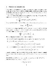
2. Sketch the probability mass function (roughly).
Binomial Dist’n: Trials = 31, Prob of success = 0.447
Probability Mass
0.00 0.08
5 10 15 20
Number of Successes
3. Sketch the cumulative distribution function (roughly).
Binomial Dist’n: Trials = 31, Prob of success = 0.447
Cumulative Probability
0.0 0.4 0.8
5 10 15 20 25
Number of Successes

5.7. FUNCTIONS OF DISCRETE RANDOM VARIABLES 133
4. Find the probability that X is equal to 17.
> dbinom(17, size = 31, prob = 0.447)
[1] 0.07532248
5. Find the probability that X is at most 13.
> pbinom(13, size = 31, prob = 0.447)
[1] 0.451357
6. Find the probability that X is bigger than 11.
> pbinom(11, size = 31, prob = 0.447, lower.tail = FALSE)
[1] 0.8020339
7. Find the probability that X is at least 15.
> pbinom(14, size = 31, prob = 0.447, lower.tail = FALSE)
[1] 0.406024
8. Find the probability that X is between 16 and 19, inclusive.
> sum(dbinom(16:19, size = 31, prob = 0.447))
[1] 0.2544758
> diff(pbinom(c(19, 15), size = 31, prob = 0.447, lower.tail = FALSE))
[1] 0.2544758
9. Give the mean of X, denotedIEX.
> library(distrEx)
> X = Binom(size = 31, prob = 0.447)
> E(X)
[1] 13.857
10. Give the variance of X.
> var(X)
[1] 7.662921

134 CHAPTER 5. DISCRETE DISTRIBUTIONS
11. Give the standard deviation of X.
> sd(X)
[1] 2.768198
12. Find IE(4X + 51.324)
> E(4 * X + 51.324)
[1] 106.752
Exercise 5.2. For the following situations, decide what the distribution of X should be. In
nearly every case, there are additional assumptions that should be made for the distribution to
apply; identify those assumptions (which may or may not hold in practice.)
1. We shoot basketballs at a basketball hoop, and count the number of shots until we make
agoal. LetX denote the number of missed shots. On a normal day we would typically
make about 37% of the shots.
2. In a local lottery in which a three digit number is selected randomly, let X be the number
selected.
3. We drop a Styrofoam cup to the floor twenty times, each time recording whether the cup
comes to rest perfectly right side up, or not. Let X be the number of times the cup lands
perfectly right side up.
4. We toss a piece of trash at the garbage can from across the room. If we miss the trash
can, we retrieve the trash and try again, continuing to toss until we make the shot. Let X
denote the number of missed shots.
5. Working for the border patrol, we inspect shipping cargo as whenitenterstheharbor
looking for contraband. A certain ship comes to port with 557 cargo containers. Standard
practice is to select 10 containers randomly and inspect eachoneverycarefully,
classifying it as either having contraband or not. Let X count the number of containers
that illegally contain contraband.
6. At the same time every year, some migratory birds land in a bush outside for a short rest.
On a certain day, we look outside and let X denote the number of birds in the bush.
7. We count the number of rain drops that fall in a circular area onasidewalkduringaten
minute period of a thunder storm.
8. We count the number of moth eggs on our window screen.
9. We count the number of blades of grass in a one square foot patch of land.
10. We count the number of pats on a baby’s back until (s)he burps.
Exercise 5.3. Find the constant c so that the given function is a valid PDF of a random variable
X.

5.7. FUNCTIONS OF DISCRETE RANDOM VARIABLES 135
1. f (x) = Cx n , 0 < x < 1.
2. f (x) = Cxe −x , 0 < x < ∞.
3. f (x) = e −(x−C) , 7 < x < ∞.
4. f (x) = Cx 3 (1 − x) 2 , 0 < x < 1.
5. f (x) = C(1 + x 2 /4) −1 , −∞ < x < ∞.
Exercise 5.4. Show that IE(X − µ) 2 = IE X 2 − µ 2 . Hint: expand the quantity (X − µ) 2 and
distribute the expectation over the resulting terms.
Exercise 5.5. If X ∼ binom(size = n, prob = p)showthatIEX(X − 1) = n(n − 1)p 2 .
Exercise 5.6. Calculate the mean and variance of the hypergeometric distribution. Show that
µ = K M
M + N , σ2 = K MN
(M + N) 2 M + N − K
M + N − 1 . (5.7.4)