Heliostat field design for solar thermochemical processes* - SFERA

SFERA Winter School 

Solar Fuels & Materials Page 15 

Heliostat field design for solar 

thermochemical processes* 

Robert Pitz-Paal 

DLR - Solar Research 

based on: Robert Pitz-Paal, Nicolas Bayer Botero, Aldo Steinfeld Heliostat field layout 

optimization for high-temperature solar thermochemical processing Solar Energy, Volume 85, 

Issue 2, February 2011, Pages 334-343 

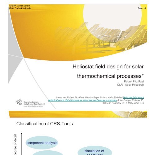
Classification of CRS-Tools 

degree of detail 

component analysis 

system analysis 

system layout 

simulation of 

operations 

optimisation of 

operations 

performance calc. 

layout optimisation 

calculation speed 

2



Maximizing annual energy 

output 

or 

Minimizing production cost 

Heliostat Field Optimization 

by variation of 

Design parameters 

heliostat position 

tower height 

receiver aperture 

… 

Operation parameters 

operation temperature 

… 

E 

S 

W 

N 

3 

Performance Calculation 

Given: Heliostat, Heliostat Positions, Aim Points, Tower, Receiver, (Secondary) 

Task: calculate annual performance 

P 

inc 

( x, 

y, 

t) 

DNI ( t) 

FMir 

refl 

atmo 

( x, 

y) 

cos( 

x, 

y, 

t) 

b& 

• coordinate systems: 

s 

( x, 

y, 

t) 

 

inc 

( x, 

y, 

t) 

• tower coordinate system 

• sun angles 

• azimuth 0° = south 

• elevation 90° = zenith 

y 

x 

• receiver coordinate systems 

4






90 

80 

70 

60 

50 

P 

inc 

( x, 

y, 

t) 

DNI ( t) 

FMir 

refl 

atmo 

( x, 

y) 

cos( 

x, 

y, 

t) 

b& 

• time system: 

9 h 

Vormittag 

10 h 

11 h 

Mittag 

12 h 

Jun 

Mai/Jul 

Apr/Aug 

Mär/Sep 

s 

( x, 

y, 

t) 

 

13 h 

inc 

Nachmittag 

14 h 

( x, 

y, 

t) 

15 h 

40 

30 

20 

6 h 

7 h 

8 h 

9 h 

10 h 

11 h 

10 

8 h 

16 h 

5 h 

0 

60 90 120 150 180 210 240 270 

Feb/Okt 

Jan/Nov 

Dez 

13 h 

14 h 

15 h 

16 h 

17 h 

18 h 

5 




P 

inc 

( x, 

y, 

t) 

DNI ( t) 

FMir 

refl 

atmo 

( x, 

y) 

cos( 

x, 

y, 

t) 

b& 

• time system: 

( x, 

y, 

t) 

 

( x, 

y, 

t) 

• 7 months: Dec, Jan/Nov, Feb/Oct, Mar/Sep, Apr/Aug, Mai/Jul, Jun 

• days/month: 31 61 59 61 61 62 60 

• one representative day per month (21st) 

• local solar time, hourly intervals 

s 

inc 

6






P 

inc 

( x, 

y, 

t) 

DNI ( t) 

FMir 

refl 

atmo 

( x, 

y) 

cos( 

x, 

y, 

t) 

b& 

• radiation model: 

• tabulated data 

• clear sky model from Hottel (1976): 

s 

( x, 

y, 

t) 

 

inc 

( x, 

y, 

t) 

DNI ( t) 

( LAT , h, 

day, 

time) 

 

atmo 

IRR ET 

850 

LAT 35°N, 0m, solar noon 

800 

DNI [W/m²] 

750 

700 

650 

600 

1 2 3 4 5 6 7 8 9 10 11 12 

7 




P 

inc 

( x, 

y, 

t) 

DNI ( t) 

FMir 

refl 

atmo 

( x, 

y) 

cos( 

x, 

y, 

t) 

b& 

• atmospheric attenuation: 

atmo 

( x, 

y) 

f ( slant range) 

1.00 

s 

( x, 

y, 

t) 

 

inc 

( x, 

y, 

t) 

• agrees well with Pittman/Vant-Hull at 

Rho_H2O 7 g/m³ 

Vis 

40 km 

H 

0 km 

h_tower 0.1 km 

Transmissivity [-] 

0.95 

0.90 

0.85 

0.80 

0.75 

0.70 

0.65 

Pitman/Vant-Hull 

HFLCAL 

0.60 

0 0.5 1 1.5 2 2.5 3 

Slant Range [km] 

8






P 

inc 

( x, 

y, 

t) 

DNI ( t) 

FMir 

refl 

atmo 

( x, 

y) 

cos( 

x, 

y, 

t) 

b& 

• cosine factor 

s 

( x, 

y, 

t) 

 

inc 

( x, 

y, 

t) 

9 




P 

inc 

( x, 

y, 

t) 

DNI ( t) 

FMir 

refl 

atmo 

( x, 

y) 

cos( 

x, 

y, 

t) 

b& 

• shading 

s 

( x, 

y, 

t) 

 

inc 

( x, 

y, 

t) 

10






P 

inc 

( x, 

y, 

t) 

DNI ( t) 

FMir 

refl 

atmo 

( x, 

y) 

cos( 

x, 

y, 

t) 

b& 

• blocking 

s 

( x, 

y, 

t) 

 

inc 

( x, 

y, 

t) 

11 

Background 

Design and optimization of solar tower systems require the 

calculation of the reflected beam in the target plane 

12



Background 

Design and optimization of solar tower systems require the 

calculation of the reflected beam in the target plane 

Deviations from ideal 

concentration: 

• non-parallel rays 

• alignment error 

• shape error 

• slope error 

• diffuse reflection 

• (off-axis-reflection) 

13 

Background 

statistical approach (ray-tracing) 

analytical approach (convolution) 

 

 

 

I M E S 

I( x, 

y) 

M ( x1 , y1) 

E( 

x2 

x1, 

y2 

y1) 

S( 

x x2, 

y y2) 

dx1dy1dx2dy2 

e 

I( 

x, 

y) 

 

2 2 

( 

x y ) 

2 

/ 2 

 

 

i0 j0 

Cij 

Hi( 

x) 

H 

j 

( y) 

i! 

j! 

14



HFLCAL Approach 

HFLCAL uses a simplified convolution approach: 

The reflected image of each heliostat is approximated by a circular normal 

distribution (“Gaussian”) 

F 

r ² 

1 

2 

² 

( ) 

r 

e 

2 

² 

 

2 

beam error 

 

2 

sun 

 

2 

beam quality 

0.035 

0.3 

0.030 

0.25 

0.025 

"Kuiper" 

probability [-] 

0.020 

0.015 

"Gaussian" 

0.2 

0.15 

0.010 

0.1 

0.005 

0.05 

0.000 

0 0.5 1 1.5 2 2.5 3 3.5 4 4.5 5 5.5 6 6.5 7 

r [mrad] 

sun 

0 

-5 -4 -3 -2 -1 0 1 2 3 4 5 

2 

mirror 

15 

Accuracy of Mathematical Model 

F 

r ² 

1 

2 

² 

( ) 

r 

e 

2 

² 

 

2 

beam error 

 

2 

sun 

 

2 

beam quality 

• Pettit, Vittitoe and Biggs (1983) found good agreement when beam error 

2 sun 

• Central Limit Theorem: „superposition of a great number of any distributions 

converges towards a normal distribution“ 

200 

200 

180 

160 

ray-tracing 

HFLCAL 

180 

160 

ray-tracing 

HFLCAL 

140 

140 

120 

120 

100 

100 

80 

80 

60 

60 

40 

40 

20 

20 

0 

-2.5 -2 -1.5 -1 -0.5 0 0.5 1 1.5 2 2.5 

perfect mirror 

0 

-2.5 -2 -1.5 -1 -0.5 0 0.5 1 1.5 2 2.5 

realistic mirror 

16




F 

r ² 

1 

2 

² 

( ) 

r 

e 

2 

² 

 

2 

beam error 

 

2 

sun 

 

2 

beam quality 

How to chose the correct value for beam error 

 

10 

4.5% 

9 

4.0% 

8 

3.5% 

total sigma [mrad] 

7 

6 

5 

4 

3 

2 

RMS (HFLCAL-RayTracing) 

3.0% 

2.5% 

2.0% 

1.5% 

1.0% 

1 

0.5% 

0 

0 0.5 1 1.5 2 2.5 3 3.5 4 4.5 5 

slope error (normal) [mrad] 

0.0% 

0 0.5 1 1.5 2 2.5 3 3.5 4 4.5 

slope error (normal) [mrad] 

total sigma 

error 

17 


tracking errors influence the amount of intercepted energy 

 

2 

beam error 

 

2 

sun 

 

2 

beam quality 

( 2 

track 

) 

2 

 

track 

 

 

 

axis1 axis2 

18




astigmatism influences the size and shape of the reflected beam 

 

2 

total 

 

2 

beam error 

 

2 

astigm 

H 

W 

t 

s 

d 

d 

SLR 

f 

SLR 

f 

cos 

; 

cos 

1; 

 

astigm 

 

1 

2 

 

H 

2 

t, 

hel 

facet 

W 

4 

SLR 

2 

s, 

hel 

facet 

 

19 


astimgatism influences the size and shape of the reflected beam 

 

2 

total 

 

2 

beam error 

 

2 

astigm 

kW/m² 

21-24 

18-21 

15-18 

12-15 

9-12 

6-9 

3-6 

0-3 

[kW/m²] 

21-24 

18-21 

15-18 

12-15 

9-12 

6-9 

3-6 

0-3 

-2.4 -1.9 -1.4 -1.0 -0.5 0.0 0.5 1.0 1.4 1.9 2.4 

-2.4 -1.9 -1.4 -1.0 -0.5 0.0 0.5 1.0 1.4 1.9 2.4 

single mirror, incident angle 37.6° (left: HFLCAL, right: ray tracing) 

20






P 

inc 

( x, 

y, 

t) 

DNI ( t) 

FMir 

refl 

atmo 

( x, 

y) 

cos( 

x, 

y, 

t) 

b& 

s 

( x, 

y, 

t) 

 

inc 

( x, 

y, 

t) 

• intercept 

 

inc 

 

1 

2 

2 

 

e 

aperture 

2 

 

 

2 

2 

2 

dd 

• aimpoint = center: analytical solution 

• aimpoint center: numerical solution 

21 




P 

inc 

( x, 

y, 

t) 

DNI ( t) 

FMir 

refl 

atmo 

( x, 

y) 

cos( 

x, 

y, 

t) 

b& 

s 

( x, 

y, 

t) 

 

inc 

( x, 

y, 

t) 

• intercept 

 

inc 

 

1 

2 

2 

 

e 

aperture 

2 

 

 

2 

2 

2 

dd 

• aimpoint = center: analytical solution 

• aimpoint center: semi-analytical solution 

22






P 

inc 

( x, 

y, 

t) 

DNI ( t) 

FMir 

refl 

atmo 

( x, 

y) 

cos( 

x, 

y, 

t) 

b& 

s 

( x, 

y, 

t) 

 

inc 

( x, 

y, 

t) 

• intercept 

 

inc 

 

1 

2 

2 

 

e 

aperture 

2 

 

 

2 

2 

2 

dd 

• free form: numerical solution 

23 




P 

rec 

( x, 

y, 

t) 

sec( 

x, 

y) 

P ( x, 

y, 

t) 

inc 

• secondary transmission 

 

 

24






• solar field power 

• thermal power 

P 

field 

( t) 

Pi 

( x, 

y, 

t) 

i 

Q 

thermal 

( t) 

P ( t) 

 

P ( t) 


conversion 

 


 

• annual performance 

E 

E 


thermal 

 

 

 

t 

w( 

t) 

P 

 

t 


w( 

t) 

Q 

( t) 

thermal 

( t) 

25 

Layout Calculation 

Given: Heliostat, Tower, Receiver, (Secondary) 

Task: calculate heliostat positions 

1. calculation of hypothetical heliostat positions 

• bilinear expansion 

• bilinear with central “gap” 

• slip planes 

• (heliostats in rows) 

• user defined algorithm 

26






1. calculation of hypothetical heliostat positions 

• bilinear expansion 

• bilinear with central “gap” 

• slip planes 

• (heliostats in rows) 

• user defined algorithm 

maximum density zone 

expand with u = au + r x bu 

slip plane: add heliostat to each gap 

27 




2. calculation of field performance 

3. selection of best performing heliostats 

28



Field Performance Matrix 

Given: Heliostat, Heliostat Positions, Tower, Receiver, (Secondary) 

Task: calculate field efficiency for any sun angle 

29 

Optimization 

Given: Heliostat, Positioning Alg., Tower, Receiver-Type, (Secondary) 

Task: optimize layout parameters 

distribute heliostats 

calculate all time points 

chose best heliostats 

optimization 

algorithm 

manipulates 

system 

parameters 

optimize for 

-power per m² reflective area 

-least cost of thermal receiver power 

30



Optimization for Power Generation vs. Chemical 

Processes 

Power Generation 

Typical temperatures below 1300 K 

Typical solar concentration 1000 suns 

Use of secondary concentrators 

Process temperature defined by 

chemical process 

Process temperature depends on solar 

power to receiver (changes over time!) 

Reactor model and chemical 

reaction characteristics 

impact field design 

31 

Assumptions to estimate theoretical upper limit 

the reactor temperature is uniform 

convection and conduction heat losses are neglected 

transient heat losses during start-up and shut-down are neglected 

reaction achieves completion, e.g. there are no chemical side products 

considered 

no purge gases are used 

32



Two Example Reactions.. 

ZnO dissociation (2000K) 

ZnO Zn + 0.5O2 

Coal gasification (1400K) 

C + H2O CO + H2 

Simplified Model Approach 

P 

P 

0 

P 

thermallosses 

solar,in 

reaction 

 

T 

 

P 

reaction 

T 

 

4 

T 

 

A T 

aperture 

P 

thermallosses 

T 

 

T 

 

( T ) 

H 

r 

( T ) cpdT 

 

 

T 

in 

Ea 

 

Areaction 

k0 

exp 

 

RT 

Target function for optimization 

 

solartochemical 

 

 

all time steps 

(T)H 

 

P 

solar, in 

all time steps 

r 

( T ) 

33 

Parameters 

Heliostat size 10 / 120 m² 

Beam Quality 

3.3; 3.0; 2.7 mrad 

incl. sunshape 

Design power 

to reactor 

1; 10; 100 MW 

Heliostat spacing 

Tower Height 

1 MW 40m 

10 MW 120m 

100 MW 250m 

34



Multimodal objective function: 

Different configurations lead to very similar optima 

Case 1 Case 2 

reflectivity 

0.87 0.87 

cosine 

0.8873 0.8863 

blockin&shading 

0.9075 0.8888 

attenuation 

0.9654 0.9688 

0.8339 0.8625 

int ercept 

secondary 

0.9146 0.9228 

receiver 

0.5868 0.5686 

0.3026836 0.3026597 

total 

35 

Results 

Comparison of fields (10MW – 10m²) 

reference field optimized for 

design point concentration of 

500 suns 

field = 69,27 % 

optimization target: chemical 

yield Coal gasification. 

field = 61,8 % 

solar-chemical =39,1% 

peak concentration = 2555 suns 

mean concentration = 2107 suns 

optimization target: chemical 

yield zinc oxide dissociation 

field = 55 % 

solar-chemical =30,6% 

peak concentration = 4798 suns 

mean concentration = 3679 suns 

36



Efficiencies [%] Reactor operating conditions 

Average Peak 

Flux 

Operating Operating 

ZnO dissociation Field Intercept Secondary Optical Reactor Total 

Density 

Temperature Temperature 

[MW/m²] 

[K] 

[K] 

1 MW 

10m2 Heliostat 

10 MW 


100 MW; 3 cavities 

120m² Heliostat 

66.7 86.4 92.1 53,1 55.5 29.5 1910 2014 4.5 

67.3 86.0 92.2 53.4 55.9 29.8 1912 2013 4.6 

63.7 88.7 91.7 51.8 57.0 29.2 1920 2017 4.8 

Efficiencies [%] 

Coal gasification Field Intercept Secondary Optical Reactor Total 

Reactor operating conditions 

Average Peak 

Flux 

Operating Operating 

Density 

Temperature Temperature 

[MW/m²] 

[K] 

[K] 

1 MW 


69.9 95.4 92.9 61.9 66.0 40.9 1308 1469 2.2 

10 MW 


69.4 95.2 93.1 61.5 66.3 40.8 1307 1470 2.9 

100 MW; 3 cavities 


65.4 96.2 93.1 58.6 66.8 39.9 1308 1483 2.5 

37 

Comparison to solar electric systems 

Thermal Receiver 

500 kW/m² 

1MW 


Efficiencies [%] 

Field Intercept Secondary Optical Reactor Total 

72.4 96.5 - 69.9 - - 

Reactor operating conditions 

10MW 


70.0 97.5 - 68.2 - 

n/a 

100MW; Northfield 


64.5 99.5 - 64.2 - - 

Chemical conversion through electrolysis: 

Assume rec 

=0.92 , 

cycle 

=0.45 , 

electrolys 

=0.8 

tot 

=0.699 *0.92* 0.45 * 0.8 = 0.23 

38



Sensitivity Analysis: Impact of beam quality 

a) d) 

The perfect 

mirror 

ZnO 

The perfect 

mirror 

C-Gasif. 

39 

Sensitivity Analysis: Impact of tower height 

b) e) 

ZnO 

C-Gasif. 

40



Sensitivity Analysis: Impact heat recovery / inlet 

temp. 

a) b) 

ZnO 

C-Gasif. 

41 

Summary 

Optimization methodology of heliostat fields for solar tower applied to hightemperature 

chemical reactions 

Application to dissociation of Zinc oxide and coal gasification with optimum 

estimation: 

Zinc oxide dissociation: 2000 K and 5000 suns 

Coal gasification: 

1400 K and 2000 suns 

Excellent secondary optics are required to achieve these conditions 

Penalties up to 25 % in field efficiencies due to need of high temperature heat of 

chemical reactions 

Systems still show efficiency benefits over solar electrochemical concepts 

High temperature reaction concepts very sensitive to beam quality and tower 

height 

42

Heliostat field design for solar thermochemical processes* - SFERA

Create successful ePaper yourself

Delete template?

Save as template?