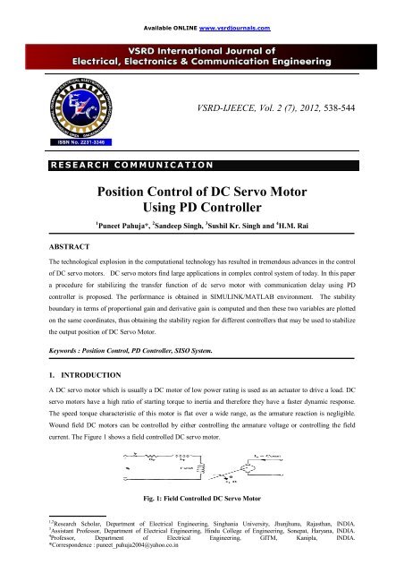
Position Control of DC Servo Motor Using PD Controller - vsrd ...

Available ONLINE www.vsrdjournals.com 

VSRD-IJEECE, Vol. 2 (7), 2012, 538-544 

R E S E A R C H C O M M U N II C A T II O N 

Position Control of DC Servo Motor 

Using PD Controller 

1 Puneet Pahuja*, 2 Sandeep Singh, 3 Sushil Kr. Singh and 4 H.M. Rai 

ABSTRACT 

The technological explosion in the computational technology has resulted in tremendous advances in the control 

of DC servo motors. DC servo motors find large applications in complex control system of today. In this paper 

a procedure for stabilizing the transfer function of dc servo motor with communication delay using PD 

controller is proposed. The performance is obtained in SIMULINK/MATLAB environment. The stability 

boundary in terms of proportional gain and derivative gain is computed and then these two variables are plotted 

on the same coordinates, thus obtaining the stability region for different controllers that may be used to stabilize 

the output position of DC Servo Motor. 

Keywords : Position Control, PD Controller, SISO System. 

1. INTRODUCTION 

A DC servo motor which is usually a DC motor of low power rating is used as an actuator to drive a load. DC 

servo motors have a high ratio of starting torque to inertia and therefore they have a faster dynamic response. 

The speed torque characteristic of this motor is flat over a wide range, as the armature reaction is negligible. 

Wound field DC motors can be controlled by either controlling the armature voltage or controlling the field 

current. The Figure 1 shows a field controlled DC servo motor. 

Fig. 1: Field Controlled DC Servo Motor 

____________________________ 

1,2 Research Scholar, Department of Electrical Engineering, Singhania University, Jhunjhunu, Rajasthan, INDIA. 

3 Assistant Professor, Department of Electrical Engineering, Hindu College of Engineering, Sonepat, Haryana, INDIA. 

4 Professor, Department of Electrical Engineering, GITM, Kanipla, INDIA. 

*Correspondence : puneet_pahuja2004@yahoo.co.in

Puneet Pahuja et al / VSRD International Journal of Electrical, Electronics & Comm. Engg. Vol. 2 (7), 2012 

Where 

e 

f 

-applied field voltage(input), 

i 

f 

-field current, 

R -field resistance, L -field inductance, 

f 

f 

Ia 

- 

armature current which is held constant, - position of shaft (taken as output). 

To design feedback control for systems with time delay, it is necessary to consider the fact that the system’s 

future behaviors depend not only on the current value of the state variables, but also some past history of the 

state variables. The method proposed in this paper involves decomposing the plant frequency response into real 

and imaginary parts and computing the stabilizing parameters for each controller based on such decomposition. 

2. FINDING THE STABILITY BOUNDS FOR PD CONTROLLERS 

Consider the SISO system shown in Figure 2. The plant (DC Servo Motor) whose position is to be controlled is 

given by : 

G ( s) G( s) 

e 

p 

s 

… (1) 

Where is the communication (time) delay. 

+ 

- 

Controller 

G ( ) c 

s 

Plant (DC 

servo motor) 

GP( s ) 

The controller used is of PD type, so : 

Fig. 2: A SISO System with Unity Feedback 

G ( s) 

K K s 

c P d 

… (2) 

The problem is to find the values of 

K 

P 

and 

Kd 

for which the closed-loop characteristic equation of the system 

( s) 1 G ( s) G ( s) 

is Hurwitz Stable. The characteristic equation in terms of j is : 

c 

P 

( j) 1 ( K jK )( R ( ) jI ( )) 

P d P P 

… (3) 

Expanding ( j) 

and setting it to zero produces : 

R ( ) I ( ) 0 

 

 

… (4) 

Where R ( ) 1 K 

PRP ( ) KdIP 

( ) 

… (5) 

Page 539 of 544


And I( ) K 

PRP ( ) KdRP 

( ) 

… (6) 

Setting the real and imaginary parts equal to zero gives : 

K ( R ( )) K ( I ( )) 1 

P P d P 

… (7) 

And K ( I ( )) K ( R 

( )) 0 

… (8) 

P P d P 

Hence, we need to solve the following system : 

RP 

( ) I 

P 

( ) KP 

1 

 

IP 

( ) RP 

( ) 

K 

 

d 

0 

 

 

… (9) 

Solving (9) for ω≠0, we obtain : 

K 

P 

( ) 

 

R ( ) 

P 

P 

G ( j) 

2 

… (10) 

IP 

( ) 

Kd 

( ) 

 

G ( j) 

P 

2 

… (11) 

Where 

P 

2 2 2 

P 

P 

G ( j) =(I ( )) +(R ( )) 

Solving (9) for ω=0, we find that K is arbitrary while : 

d 

K 

P 

1 

( ) 

 

R (0) 

P 

… (12) 

And I 

P(0) 0 

… (13) 

The lower bound in (11) will be zero except for type –zero plants. 

Again, we need to find the upper bound 

c 

that is, the point where : 

K 

( ) K (0) 

P c P 

… (14) 

For a PD controller function when 

K (0) 0 , the amount of phase that this particular controller will add at 

P 

the critical frequency to the loop transfer function is anywhere from zero to 2 

radians which leaves a range of 



3 

, 

 

 

 

2 

for the phase of the plant transfer function. Similarly, for a PD controller function when 

(0) 0 

 

K 

P 

, the amount of phase that this controller will add anywhere from to radians at the critical 

2 

frequency, which means that the phase of the plant transfer function at can be anywhere in the set 

3 

, 2 

2 

. 

In the case where the plant transfer function is a type-one system or higher, K 

P(0) 0 will hold, resulting in 

the controller phase angle of 2 

radians at 

 

c 

and the plant transfer function phase of 

c 

3 

2 

radians at the 

critical frequency. To design PD controllers that will satisfy specific gain and phase margins, a test function 

Ggp 

 

j 

Ae 

is inserted in the feed forward path as shown Figure 3. [1] 

…(15) 

Fig. 3 : A Basic Control System With A Test Function 

Then, G ( j) G( j) e Ae G( j) 

e 

P 

j j j 

… (16) 

Where G ( j) AG( j) 

… (17) 

And 

… (18) 

3. CASE STUDY 

The transfer function of the plant i.e. a typical DC servo motor taking shaft position as output and field voltage 

as input is[2]; 

m( s) 1 

 

v 

f 

( s) s s 

1 

G(s) = 

… (19) 

For the communication delay of 1 : 



s 1 1s 

Gp 

( s) G( s) 

e 

 

e 

s( s 1) 

… (20) 

We proceed with using equation (2) as the controller function. To obtain the values for 

K 

P 

and 

K 

d 

, we 

decompose equation (16) into real and imaginary parts and substitute them into equation (10) and (11) where 

 

 

0, c 

 

. 

Now we find the set of all stabilizing PD controllers for the DC Servo Motor such that the gain margin is greater 

than or equal to 2 and the phase margin is greater than or equal to 4 

. The frequency response is for the motor 

input voltage to the shaft angular position. The magnitude and phase plots of the motor are displayed in Figure 

4. 

40 

20 

Bode Diagram 

Magnitude (dB) 

0 

-20 

-40 

-60 

-80 

Phase (deg) 

-90 

-135 

-180 

-225 

-270 

-315 

-360 

System: DCServoMotor 

Frequency (rad/sec): 2.02 

Phase (deg): -270 

10 -2 10 -1 10 0 10 1 

Frequency (rad/sec) 

System: DCServoMotor 

Frequency (rad/sec): 0.863 

Phase (deg): -180 

Fig. 4 : Bode plot of DC Servo Motor 

The general stability boundary locus is first computed, i.e., the locus when A=1 and θ=0. To design the 

controllers that satisfy the gain margin condition, set A=2 and θ=0 in equation (16). Then, from the given 

frequency response, extract the real and imaginary values at each ω and substitute it into equations (10) and 

(11) to obtain the stability boundary. To satisfy the criterion for the phase margin, repeat the procedure, but 

 

with A=1 and θ= . The results are shown in Figure 5. 

4 



2 

1.8 

1.6 

GM = 1; PM = 0 

GM = 1, PM = /4 

GM = 2, PM = 0 

1.4 

1.2 

K p 

1 

0.8 

0.6 

0.4 

0.2 

0 

-1 -0.5 0 0.5 1 1.5 2 2.5 

K d 

Fig. 5 : Stability Region For Required Gain And Phase Margin 

To verify the results use the closed loop simulation of Figure 6. We chose 

K 

P 

=0.4 and 

K 

d 

=0.5 and tested the 

0 

response of the motor to a step input of 45 . From Figure 7 we find that the closed-loop system is indeed stable. 

Fig. 6 : Simulation Diagram To Verify The Results 

50 

45 

40 

Angular Position(degrees) 

35 

30 

25 

20 

15 

10 

5 

0 

0 5 10 15 20 25 30 

Time(Seconds) 

Fig. 7 : Step Response of the DC Servo Motor with desired values of Gain and Phase Margin 



4. CONCLUSION 

After a number of repeated simulations in Matlab it is found that the given values of ( K , K ) stabilize the 

transfer function of the given DC servo motor. The case study is done. The results are useful to make the 

controller design for the Position control of DC Servo Motor. 

p 

d 

5. FUTURE SCOPE 

The same procedure can be used to find gains for PID controller, for controller design of Positon control of DC 

Servo Motor. The work can be extended to design the robust PID controllers. 

6. REFERENCES 

[1] Tan., N. (2005): Computation of stabilizing PI and PID controllers for the processes with time delay, ISA 

Transactions, vol. 44. 

[2] Houpis, C. H. and Rasmussen, Steven J (1999): Quantitive Feedback Theory Fundamentals and 

Applications, Marcel Dekker Inc. New york Bassel. 

[3] Rai,, H.M. (2003):Control System Engineering, Satya Prakashan . 

[4] Silva, Guillermo J., Datta, Aniruddha, and Bhattacharya, S.P. (2005): PID controllers for Time-Delay 

Systems, Birkhauser. 

[5] Sujoldzic,S. and Watkins, J.M.(2005): Stabilization of an arbitrary order transfer function with time delsy 

using PID controllers, Proc. Of IEEE conf. on Decision and Control.

Position Control of DC Servo Motor Using PD Controller - vsrd ...

You also want an ePaper? Increase the reach of your titles

Delete template?

Save as template?