Packet-pair bandwidth estimation: stochastic analysis of a ... - ICNP

Packet-Pair Bandwidth Estimation: Stochastic
Analysis of a Single Congested Node
1 Seong-ryong Kang, 2 Xiliang Liu, 1 Min Dai, and 1 Dmitri Loguinov
1 Texas A&M University, College Station, TX 77843, USA
{skang, dmitri}@cs.tamu.edu, min@ee.tamu.edu
2 City University of New York, New York, NY 10016, USA
xliu@gc.cuny.edu
Abstract— In this paper, we examine the problem of estimating
the capacity of bottleneck links and available bandwidth of endto-end
paths under non-negligible cross-traffic conditions. We
present a simple stochastic analysis of the problem in the context
of a single congested node and derive several results that allow the
construction of asymptotically-accurate bandwidth estimators.
We first develop a generic queuing model of an Internet router
and solve the estimation problem assuming renewal cross-traffic
at the bottleneck link. Noticing that the renewal assumption on
Internet flows is too strong, we investigate an alternative filtering
solution that asymptotically converges to the desired values of
the bottleneck capacity and available bandwidth under arbitrary
(including non-stationary) cross-traffic. This is one of the first
methods that simultaneously estimates both types of bandwidth
and is provably accurate. We finish the paper by discussing the
impossibility of a similar estimator for paths with two or more
congested routers.
I. INTRODUCTION
Bandwidth estimation has recently become an important
and mature area of Internet research [1], [2], [4], [5], [6],
[7], [10], [11], [12], [14], [15], [16], [18], [19], [20], [21],
[22], [23], [24], [25], [26], [27]. A typical goal of these
studies is to understand the characteristics of Internet paths
and those of cross-traffic through a variety of end-to-end
and/or router-assisted measurements. The proposed techniques
usually fall into two categories – those that estimate the
bottleneck bandwidth [4], [5], [6], [12], [13] and those that
deal with the available bandwidth [11], [19], [24], [26]. Recall
that the former bandwidth metric refers to the capacity of the
slowest link of the path, while the latter is generally defined
as the smallest average unused bandwidth among the routers
of an end-to-end path.
The majority of existing bottleneck-bandwidth estimation
methods are justified assuming no cross-traffic along the path
and are usually examined in simulations/experiments to show
that they can work under realistic network conditions [4],
[5], [6], [7], [12]. With available bandwidth estimation, crosstraffic
is essential and is usually taken into account in the
analysis; however, such analysis predominantly assumes a fluid
model for all flows and implicitly requires that such models be
accurate in non-fluid cases. Simulations/experiments are again
used to verify that the proposed methods are capable of dealing
with bursty conditions of real Internet cross-traffic [11], [19],
[24], [26].
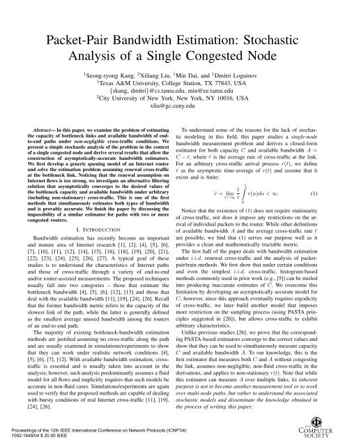
To understand some of the reasons for the lack of stochastic
modeling in this field, this paper studies a single-node
bandwidth measurement problem and derives a closed-form
estimator for both capacity C and available bandwidth A =
C − ¯r, where ¯r is the average rate of cross-traffic at the link.
For an arbitrary cross-traffic arrival process r(t), we define
¯r as the asymptotic time-average of r(t) and assume that it
exists and is finite:
∫
1
t
¯r = lim r(u)du < ∞. (1)
t→∞ t
0
Notice that the existence of (1) does not require stationarity
of cross-traffic, nor does it impose any restrictions on the arrival
of individual packets to the router. While other definitions
of available bandwidth A and the average cross-traffic rate ¯r
are possible, we find that (1) serves our purpose well as it
provides a clean and mathematically tractable metric.
The first half of the paper deals with bandwidth estimation
under i.i.d. renewal cross-traffic and the analysis of packetpair/train
methods. We first show that under certain conditions
and even the simplest i.i.d. cross-traffic, histogram-based
methods commonly used in prior work (e.g., [5]) can be misled
into producing inaccurate estimates of C. We overcome this
limitation by developing an asymptotically accurate model for
C; however, since this approach eventually requires ergodicity
of cross-traffic, we later build another model that imposes
more restriction on the sampling process (using PASTA principles
suggested in [26]), but allows cross-traffic to exhibit
arbitrary characteristics.
Unlike previous studies [26], we prove that the corresponding
PASTA-based estimators converge to the correct values and
show that they can be used to simultaneously measure capacity
C and available bandwidth A. To our knowledge, this is the
first estimator that measures both C and A without congesting
the link, assumes non-negligible, non-fluid cross-traffic in the
derivations, and applies to non-stationary r(t). Note that while
this estimator can measure A over multiple links, its inherent
purpose is not to become another measurement tool or to work
over multi-node paths, but rather to understand the associated
stochastic models and disseminate the knowledge obtained in
the process of writing this paper.
Proceedings of the 12th IEEE International Conference on Network Protocols (ICNP’04)
1092-1648/04 $ 20.00 IEEE

We conclude the paper by discussing the impossibility
of building an asymptotically optimal estimator of both C
and A for a two-node case. While estimation of A may
be possible for multi-node paths, our results suggest that
provably-convergent estimators of C do not exist in the context
of end-to-end measurement. Thus, the problem of deriving a
provably accurate estimator for a two-node case with arbitrary
cross-traffic remains open; however, we hope that our initial
work in this direction will stimulate additional research and
prompt others to prove/disprove this conjecture.
II. STOCHASTIC QUEUING MODEL
In this section, we build a simple model of a router that
introduces random delay noise into the measurements of the
receiver and use it to study the performance of packet-pair
bandwidth-sampling techniques. Note that we depart from the
common assumption of negligible and/or fluid cross-traffic and
specifically aim to understand the effects of random queuing
delays on the bandwidth sampling process. First consider an
unloaded router with no cross-traffic. The packet-pair mechanism
is based on an observation that if two packets arrive at the
bottleneck link with spacing x smaller than the transmission
delay ∆ of the second packet over the link, their spacing after
the link will be exactly ∆. In practice, however, packets from
other flows often queue between the two probe packets and
increase their spacing on the exit from the bottleneck link to
be larger than ∆.
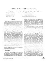
Assume that packets of the probe traffic arrive to the
bottleneck router at times a 1 , a 2 ,...and that inter-arrival times
a n − a n−1 are given by a random process x n determined by
the server’s initial spacing. Further assume that the bottleneck
node delays arriving packets by adding a random processing
time ω n to each received packet n. For the remainder of the
paper, we use constant 1 packet size q for the probing flow and
arbitrarily-varying packet sizes for cross-traffic. Furthermore,
there is no strict requirement on the initial spacing x n as long
as the modeling assumptions below are satisfied. This means
that both isolated packet pairs or bursty packet trains can be
used to probe the path. Let the transmission delay of each
application packet through the bottleneck link be q/C =∆,
where C is the transmission capacity of the link. Under these
assumptions, packet departure times d n are expressed by the
following recurrence 2 :
{
a1 + ω 1 +∆ n =1
d n =
max(a n ,d n−1 )+ω n +∆ n ≥ 2 . (2)
In this formula, the dependence of d n on departure time
d n−1 is a consequence of FIFO queuing (i.e., packet n cannot
depart before packet n − 1 is fully transmitted). Furthermore,
packet n cannot start transmission until it has fully arrived
(i.e., time a n ). The value of the noise term ω n is proportional
to the number of packets generated by cross-traffic and queued
1 Methods that vary the probing packet size also exist (e.g., [6], [10]).
2 Times d n specify when the last bit of the packet leaves the router.
Similarly, times a n specify when the last bit of the packet is fully received
and the packet is ready for queuing.
arrival
departure
time
Fig. 1.
Departure delays introduced by the node.
in front of packet n. The final metric of interest is interdeparture
delay y n = d n − d n−1 as the packets leave the
router. The various variables and packet arrival/departure are
schematically shown in Figure 1.
Even though the model in (2) appears to be simple, it
leads to fairly complicated distributions for y n if we make no
prior assumptions about cross-traffic. We next examine several
special cases and derive important asymptotic results about
process y n .
A. Packet-Pair Analysis
III. RENEWAL CROSS-TRAFFIC
We start our analysis with a rather common assumption in
queuing theory that cross-traffic arrives into the bottleneck link
according to some renewal process (i.e., delays between crosstraffic
packets are i.i.d. random variables). In what follows
in the next few subsections, we show that modeling of this
direction requires stationarity (more specifically, ergodicity) of
cross-traffic. However, since neither the i.i.d. assumption nor
stationarity holds for regular Internet traffic, we then apply
a different sampling methodology and a different analytical
direction to derive a provably robust estimator of capacity C
and average cross-traffic rate ¯r.
The goal of bottleneck bandwidth sampling techniques is to
queue probe packets directly behind each other at the bottleneck
link and ensure that spacing y n on the exit from the router
is ∆. In practice, however, this is rarely possible when the
rate of cross-traffic is non-negligible. This does present certain
difficulties to the estimation process; however, assuming a
single congested node, the problem is asymptotically tractable
given certain mild conditions on cross-traffic. We present these
results below.
To generate measurements of the bottleneck capacity, it is
commonly derived that the server must send its packets with
initial spacing no more than ∆ (i.e., no slower than C). This is
true for unloaded links; however, when cross-traffic is present,
the probes may be sent arbitrarily slower as long as each
packet i arrives to the router before the departure time of
packet i − 1. This condition translates into a n ≤ d n−1 and
Proceedings of the 12th IEEE International Conference on Network Protocols (ICNP’04)
1092-1648/04 $ 20.00 IEEE

(2) expands to:
d n =
{
a1 + ω 1 +∆ n =1
d n−1 + ω n +∆ n ≥ 2 . (3)
From (3), packet inter-departure times y n after the bottleneck
router are given by:
y n = d n − d n−1 =∆+ω n , n ≥ 2. (4)
Notice that random process ω n is defined by the arrival
pattern of cross-traffic and also by its packet-size distribution.
Since this process is a key factor that determines the distribution
of sampled delays y n , we next focus on analyzing its
properties. Assume that inter-packet delays of cross-traffic are
given by independent random variables {X i } and the actual
arrivals occur at times X 1 ,X 1 + X 2 ,... Thus, the arrival
pattern of cross-traffic defines a renewal process M(t), which
is the number of packet arrivals in the interval [0,t]. Using
common convention, further assume that the mean inter-arrival
delay E[X i ] is given by 1/λ, where λ =¯r is the mean arrival
rate of cross-traffic in packets per second.
To allow random packet sizes, assume that {S j },j =
1, 2,...are independent random variables modeling the size of
packets in cross-traffic. We further assume that the bottleneck
link is probed by a sequence of packet-pairs, in which the
delay between the packets within each pair is small (so as
to keep their rate higher than C) and the delay between the
pairs is high (so as not to congest the link). Under these
assumptions, the amount of cross-traffic data received by the
bottleneck link between probe packets 2m − 1 and 2m (i.e.,
in the interval (a 2m−1 ,a 2m ]) is given by a cumulative reward
process:
v n =
M(a n)−M(a
∑ n−1)
j=1
S j , n =2m, (5)
where n represents the sequence number of the second packet
in each pair. For now, we assume a general (not necessarily
equilibrium) process M(t) and re-write (4) as:
M(a n )−M(a
∑ n−1 )
y n =∆+ v S j
n
C =∆+ j=1
, n =2m. (6)
C
Since classical renewal theory is mostly concerned with
limiting distributions, y n by itself does not lead to any tractable
results because the observation period of the process captured
by each of y n is very small.
Define a time-average process W n to be the average of {y i }
up to time n:
W n = 1 n∑
y i . (7)
n
Then, we have the following result.
Claim 1: Assuming ergodic cross-traffic, time-average process
W n converges to:
lim W n =∆+ λE[x n]E[S j ]
=∆+E[ω n ], (8)
n→∞ C
i=1
Snd1
100 mb/s
100 mb/s
1.5 mb/s
R 1
R 2
Snd2
100 mb/s
Fig. 2.
100 mb/s
Rcv1
Rcv2
Single-link simulation topology.
where E[x n ] is the mean inter-probe delay of packet-pairs.
Proof: Process W n samples a much larger span of
M(t) and has a limiting distribution as we demonstrate below.
Applying Wald’s equation to (6) [28]:
E [y n ]=∆+ E[M(a n) − M(a n−1 )]E[S j ]
. (9)
C
The last result holds since M(t) and S j are independent
and M(a n ) − M(a n−1 ) is a stopping time for sequence
{S j }. Equation (9) can be further simplified by noticing that
E[M(t)] is the renewal function m(t):
E [y n ]=∆+ (m(a n) − m(a n−1 ))E[S j ]
. (10)
C
Assuming stationary cross-traffic, (10) expands to [28]:
E [y n ]=∆+ λE[x n]E[S j ]
. (11)
C
Finally, assuming ergodicity of cross-traffic (which implies
that of process y n ), we can obtain (11) using a large number
of packet pairs as the limit of W n in (7) as n →∞.
Notice that the second term in (8) is strictly positive under
the assumptions of this paper. This leads to an interesting
observation that the filtering problem we are facing is quite
challenging since the sampled process y n represents signal
∆ corrupted by a non-zero-mean noise ω n . This is a drastic
departure from the classical filter theory, which mostly deals
with zero-mean additive noise. It is also interesting that the
only way to make the noise zero-mean is to either send probe
traffic with E[x n ]=0(i.e., infinitely fast) or to have no crosstraffic
at the bottleneck link (i.e., λ =¯r =0). The former case
is impossible since x n is always positive and the latter case is
a simplification that we explicitly want to avoid in this work.
We will present our analysis of packet-train probing shortly,
but in the mean time, discuss several simulations to provide
an intuitive explanation of the results obtained so far.
B. Simulations
Before we proceed to estimation of C, let us explain several
observations made in previous work and put them in the
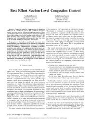
context of our model in (6) and (8). For the simulations in this
section, we used the ns2 network simulator with the topology
shown in Fig. 2. In the figure, the source of probe packets
Snd1 sends its data to receiver Rcv1 across two routers R 1
and R 2 . The speed of all access links is 100 mb/s (delay 5 ms),
Proceedings of the 12th IEEE International Conference on Network Protocols (ICNP’04)
1092-1648/04 $ 20.00 IEEE

0.6
0.5
0.4
0.3
0.2
0.15
0.25
0.2
frequency
0.4
0.3
frequency
0.2
frequency
0.1
frequency
0.15
0.1
0.2
0.1
0.1
0.05
0.05
0
8 9 10 11 12 13 14 15
values of y(n) (ms)
0
10 15 20 25
values of y(n) (ms)
0
8 10 12 14 16 18 20
values of y(n) (ms)
0
10 15 20
values of y(n) (ms)
(a) ¯r =1mb/s
(b) ¯r =1.3 mb/s
(a) ¯r = 750 kb/s
(b) ¯r =1mb/s
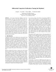
The histogram of measured inter-arrival times y n under CBR cross-
Fig. 3.
traffic.
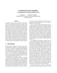
The histogram of measured inter-arrival times y n under TCP cross-
Fig. 4.
traffic.
while the bottleneck link R 1 → R 2 has capacity C =1.5 mb/s
and 20 ms delay. Note that there are five cross-traffic sources
attached to Snd2.
We next discuss simulation results obtained under UDP
cross-traffic. In the first case, we initialize all five sources
in Snd2 to be CBR streams, each transmitting at 200 kb/s
(¯r =1mb/s total cross-traffic). Each CBR flow starts with
a random initial delay to prevent synchronization with other
flows and uses 500-byte packets. The probe flow at Snd1
sends its data at an average rate of 500 kb/s for the probing
duration, which results in 100% utilization of the bottleneck
link. In the second case, we lower packet size of cross-traffic to
300 bytes and increase its total rate to 1.3 mb/s to demonstrate
more challenging scenarios when there is packet loss at the
bottleneck.
These simulation results are summarized in Fig. 3, which
illustrates the distribution of the measured samples y n based
on each pair of packets sent with spacing x n ≤ ∆ (the results
exclude packet pairs that experienced loss). Given capacity
C =1.5 mb/s and packet size q =1, 500 bytes, the value of
∆ is 8 ms. Fig. 3 shows that none of the samples are located
at the correct value of 8 ms and that the mean of the sampled
signal (i.e., W n ) has shifted to 11.7 ms for the first case and
14.5 ms for the second one.
Next, we employ TCP cross-traffic, which is generated
by five FTP sources attached to Snd2. The TCP flows use
different packet sizes of 540, 640, 840, 1,040, and 1,240 bytes,
respectively. The histogram of y n for this case is shown in Fig.
4 for two different average cross-traffic rates ¯r = 750 kb/s and
¯r =1mb/s. As seen in the figure, even though some of the
samples are located at 8 ms, the majority of the mass in the
histogram (including the peak modes) are located at the values
much higher than 8 ms.
Recall from (8) that W n of the measured signal tends to
∆+E[ω n ]. Under CBR cross-traffic, we can estimate the mean
of the noise E[ω n ] to be approximately 11.7 − 8=3.7 ms in
the first case and 14.5−8 =6.5 ms in the second one. The two
naive estimates of C based on W n are ˜C = q/W n =1, 025
kb/s and ˜C = 827 kb/s, respectively. Likewise, for the TCP
case, the measured averages (i.e., 12.2 and 13.3 ms each) of
samples y n lead to incorrect naive estimates ˜C = 983 kb/s
and ˜C = 902 kb/s, respectively.
In order to understand how ˜C and the value of W n evolve,
we run another simulation under 1 mb/s total TCP cross-traffic
and plot the evolutions of the absolute error | ˜C−C| and that of
W n in Fig. 5. As Fig. 5(a) shows, the absolute error between
C and ˜C converges to a certain value after 5,000 samples y n ,
providing a rather poor estimate ˜C ≈ 1, 010 kb/s. Fig. 5(b)
illustrates that W n in fact converges to ∆+E[ω n ], where the
mean of the noise is W n − ∆ ≈ 11.9 − 8=3.9 ms.
Previous work [1], [4], [5], [15], [22] focused on identifying
the peaks (modes) in the histogram of the collected bandwidth
samples and used these peaks to estimate the bandwidth;
however, as Figs. 3 and 4 show, this can be misleading when
the distribution of the noise is not known a-priori. For example,
the tallest peak on the right side of Fig. 3 is located at 13 ms
( ˜C = 923 kb/s), which is only a slightly better estimate than
827 kb/s derived from the mean of y n . Moreover, the tallest
peak in Fig. 4(a) is located at 14.5 ms, which leads to a worse
estimate ˜C = 827 kb/s compared to 983 kb/s computed from
the mean of y n .
To combat these problems, existing studies [1], [4], [5], [15],
[22] apply numerous empirical methods to find out which
mode is more likely to be correct. This may be the only
feasible solution in multi-hop networks; however, one must
keep in mind that it is possible that none of the modes in the
measured histogram corresponds to ∆ as evidenced by both
graphs in Fig. 3.
C. Packet-Train Analysis
Another topic of debate in prior work was whether packettrain
methods offer any benefits over packet-pair methods.
Some studies suggested that packet-train measurements converge
to the available bandwidth 3 for sufficiently long bursts
of packets [1], [4]; however, no analytical evidence to this
effect has been presented so far. Other studies [5] employed
packet-train estimates to increase the measurement accuracy
of bottleneck bandwidth estimation, but it is not clear how
these samples benefit asymptotic convergence of the estimation
process.
We consider a hypothetic packet-train method that transmits
probe traffic in bursts of k packets and averages the interpacket
arrival delays within each burst to obtain individual
3 Even though this question appears to have been settled in some of the
recent papers, we provide additional insight into this issue.
Proceedings of the 12th IEEE International Conference on Network Protocols (ICNP’04)
1092-1648/04 $ 20.00 IEEE

Absolute error (kb/s)
495
490
485
480
Average sample values (ms)
11.95
11.9
11.85
11.8
11.75
frequency
0.4
0.3
0.2
0.1
frequency
0.5
0.4
0.3
0.2
0.1
0 1 2 3
Number of samples
x10 4
0 1 2 3
Number of samples
x10 4
0
10 15 20 25
values of y(n) (ms)
0
10 15 20 25
values of y(n) (ms)
(a) | ˜C − C|
(b) W n
(a) k =5
(b) k =10
Fig. 5. (a) The absolute error of the packet-pair estimate under TCP crosstraffic
of ¯r =1mb/s. (b) Evolution of W n.
Fig. 6. The histogram of measured inter-arrival times Zn k based on packet
trains and CBR cross-traffic of ¯r =1.3 mb/s.
samples {Zn}, k where n is the burst number. For example, if
k =10, samples y 2 ,...,y 10 define Z1 10 , samples y 12 ,...,y 20
define Z2 10 , and so on. The reason for excluding samples
y 1 ,y n+1 ,...,y nk+1 is because they are based on the leading
packets of each burst, which encounter large inter-burst gaps
in front of them and do not follow the model developed so
far.
In what follows in this section, we derive the distribution
of {Zn} k as k →∞.
Claim 2: For sufficiently large k, constant x n = x, and a
regenerative processes M(t), packet-train samples converge to
the following Gaussian distribution for large n:
{
Z
k
n
} D
−→ N
(
, λxV ar[S j − λE[S j ]X i ]
)
(k − 1)C 2 ,
∆+ λxE[S j]
C
(12)
where −→ D
denotes convergence in distribution, N(µ, σ) is a
Gaussian distribution with mean µ and standard deviation σ,
and X i are inter-packet arrival delays of cross-traffic.
Proof: First, define a k-sample version of the cumulative
reward process in (5):
V k n =
M(a kn )−M(a k(n−1)+1 )
∑
j=1
S j , n =1, 2,.... (13)
Process Vn
k is also a counting process, however, its timescale
is measured in bursts instead of packets. Thus, Vn
k
determines the amount of cross-traffic data received by the
bottleneck link during an entire burst n. Equation (13) shows
that Zn k can be asymptotically interpreted as the reward rate
of the reward-renewal process Vn k :
Z k n =∆+
V k n
(k − 1)C , (14)
where k − 1 is the number of inter-packet gaps in a k-packet
train of probe packets. Assuming M(t) is regenerative and for
sufficiently large k, we have [28]:
Z k n =∆+
V1
k
+ o(1). (15)
(k − 1)C
Applying the regenerative central limit theorem, constraining
the rest of the derivations in this section to constant
x n = x, and assuming E[X i ] < ∞ [28]:
{ } V
k (
1 D
−→ N
k − 1
λxE[S j ], λxV ar[S j − λE[S j ]X i ]
k − 1
(16)
Combining (15) and (16), we get (12).
First, notice that the mean of this distribution is the same
as that of samples {y n } in (11), which, as was intuitively
expected, means that both measurement methods have the
same expectation. Second, it is also easy to notice that the
variance of Zn k tends to zero as long as Var[X i ] is finite.
Claim 3: If Var[X i ] is finite, the variance of packet-train
samples Zn k tends to zero for large k.
Proof: Since λ, x, and E[S j ] are all finite and do not
depend on k, using independence of S j and X i in (12), we
have:
( λxV
Var[Zn]=
k ar[Sj ]+λ 3 xE 2 ) 2
[S j ]Var[X i ]
(k − 1)C 2 , (17)
which tends to 0 for k →∞.
As a result of this phenomenon, longer packet trains will
produce narrower distributions centered at ∆+E[ω n ]. The
CBR case already studied in Fig. 3(b) clearly has finite
Var[X i ] and therefore samples {Zn} k must exhibit decaying
variance as k increases. One example of this convergence for
packet trains with k =5and k =10is shown in Fig. 6.
D. Discussion
Now we address several observations of previous work.
It is noted in [5] that while packet-pair histograms usually
have many different modes, the histogram of packet-train
samples becomes unimodal with increased k. This readily
follows from (12) and the Gaussian shape of {Zn}. k Previous
papers also noted (e.g., [5]) that as packet-train size k is
increased, the distribution of samples {Zn} k exhibits lower
variance. This result follows from the above discussion and
(17). Furthermore, [5] found that packet-train histograms for
large k tend to a single mode whose location is “independent
of burst size k.” Our derivations provide an insight into how
this process happens and shows the location of this “single
mode” to be ∆+E[ω n ] in (12).
In summary, packet-train samples {Zn} k represent a limited
reward rate that asymptotically converges to a Gaussian distribution
with mean E[y n ]. Perhaps it is possible to infer some
)
.
Proceedings of the 12th IEEE International Conference on Network Protocols (ICNP’04)
1092-1648/04 $ 20.00 IEEE

characteristics of {X i } by observing the variance of {Z k n} and
applying the result in (12); however, since there are several
unknown parameters in the formula (such as Var[X i ] and
E[S j ]), this direction does not lead to any tractable results
unless we assume a particular process M(t).
Since {Z k n} asymptotically tend to a very narrow Gaussian
distribution centered at ∆+E[ω n ], we find that there is no
evidence that {Z k n} measure the available bandwidth or offer
any additional information about the value of ∆ as compared
to traditional packet-pair samples {y n }.
IV. ARBITRARY CROSS-TRAFFIC
In this section, we relax the stationarity and renewal assumptions
about cross-traffic and derive a robust estimator of
C and ¯r. Assume an arbitrary arrival process r(t) for crosstraffic,
where r(t) is its instantaneous rate at time t. We impose
only one constraint on this process – it must have a finite time
average ¯r shown in (1). The goal of the sampling process
is to determine both C and ¯r. Since ¯r >Cimply constant
packet loss and zero available bandwidth, we are generally
interested in non-trivial cases of ¯r ≤ C. Stochastic process
r(t) may be renewal, regenerative, a superposition of ON/OFF
sources, self-similar, or otherwise. Furthermore, since packet
arrival patterns in the current Internet commonly exhibit nonstationarity
(due to day-night cycles, routing changes, link
failure, etc.), our assumptions on r(t) allow us to model a
wide variety of such non-stationary processes and are much
broader than commonly assumed in traffic modeling literature.
Next, notice that if the probing traffic can sample r(t) using
a Poisson sequence of probes at times t 1 ,t 2 ,..., the average
of r(t i ) converges to ¯r (applying the PASTA principle [28]):
∫
r(t 1 )+r(t 2 )+... + r(t n ) 1
t
lim
= lim r(u)du =¯r,
n→∞
n
t→∞ t
0
(18)
as long as delays τ i = t i − t i−1 are i.i.d. exponential random
variables. In order to accomplish this type of sampling, the
sender must emit packet-pairs at exponentially distributed
intervals. Assuming that the i-th packet-pair arrives to the
router at time t i , it will sample a small segment of r(t) by
allowing g i amount of data to be queued between the probes:
g i =
t∫
i +x i
t i
r(u)du ≈ r(t i )x i , (19)
where x i is the spacing between the packets in the i-th packetpair.
Again, assuming that y i is the i-th inter-arrival sample
generated by the receiver, we have:
y i =∆+ g i
C =∆+r(t i)x i
C . (20)
Finally, fixing the value of x i = x, notice that W n has a
well-defined limit:
lim W 1
n = lim
n→∞ n→∞ n
n∑
i=1
= ∆+ x C lim
(
∆+ r(t )
i)x i
C
n∑
n→∞
i=1
r(t i )
n
=∆+x¯r
C . (21)
In essence, this result 4 is similar to our earlier derivations,
except that (21) requires much weaker restrictions on crosstraffic
and also shows that a single-node model is completely
tractable in the setting of almost arbitrary cross-traffic. We
next show how to extract both C and ¯r from (21).
A. Capacity
Observe that (21) is a linear function of x, where ¯r is the
slope and ∆ is the intercept 5 . Therefore, by injecting packetpairs
with two different spacings x a and x b , one can compute
the unknown terms in (21) using two sets of measurements
{yi a} and {yb i }. To accomplish this, define the corresponding
average processes to be Wn a and Wn:
b
Wn a = 1 n∑
yi a , Wn b = 1 n∑
yi b . (22)
n
n
i=1
The simplest way to obtain both Wn a and Wn b using a
single measurement is to alternate spacing x a and x b while
preserving the PASTA sampling property. Using a one-bit
header field, the receiver can unambiguously sort the interarrival
delays into two sets {yi a} and {yb i }, and thus compute
their averages in (22).
While samples are being collected, the receiver has two
running averages produced by (22). Subtracting Wn b from Wn a ,
we are able to separate ¯r/C from ∆:
i=1
lim (W n a − Wn)= b (x a − x b )¯r
. (23)
n→∞ C
Next, denote by ˜∆ n the following estimate of ∆ at time n:
˜∆ n = Wn a Wn a − Wn
b − x a . (24)
x a − x b
Taking the limit of (24), we have the following result.
Claim 4: Assuming a single congested bottleneck for which
time-average rate ¯r exists, ˜∆n converges to ∆:
lim ˜∆ n =∆. (25)
n→∞
Proof: Re-writing (25):
lim ˜∆ n =∆+ x a¯r
n→∞
C
− x (x a − x b )¯r
a
=∆, (26)
C(x a − x b )
which is obtained with the help of (21), (23), and (24).
Our next result shows a more friendly restatement of the
previous claim.
4 A similar formula has been derived in [3], [8], [19] and several other
papers under a fluid assumption.
5 For technical differences between this approach and previous work (such
as TOPP [19]), see [17].
Proceedings of the 12th IEEE International Conference on Network Protocols (ICNP’04)
1092-1648/04 $ 20.00 IEEE

TABLE I
AVAILABLE BANDWIDTH ESTIMATION ERROR
Bottleneck capacity
Relative error
C (mb/s) Model (29) Pathload Spruce IGI
1.5 8.6% 46.5% 27.9% 84.5%
5 8.3% 40.1% 23.4% 90.0%
10 10.1% 40.9% 26.9% 89.0%
15 7.7% 38.5% 24.5% 83.1%
Corollary 1: Assuming a single congested bottleneck for
which time-average rate ¯r exists, estimate ˜C n = q/ ˜∆ n
converges to capacity C:
lim ˜C n = lim
n→∞
n→∞
B. Available Bandwidth
= lim
n→∞
q
Wn a Wn − x a−W n
b a x a−x b
q(x a − x b )
x a W b n − x b W a n
= C. (27)
Notice that knowing an estimate of C in (27) and using ¯r
in (23), it is easy to estimate the mean rate of cross-traffic:
(Wn a − W
lim
n) b ˜C n
=¯r, (28)
n→∞ x a − x b
which leads to the following result.
Corollary 2: Assuming a single congested bottleneck for
which time-average rate ¯r exists, the following converges to
the available bandwidth A = C − ¯r:
(
lim q xa − x b − Wn a + W b )
n
n→∞ x a Wn b − x b Wn
a = C − ¯r = A. (29)
C. Simulations
We confirm these results and compare our models with
several recent methods spruce [26], IGI [8], and pathload
[12] through ns2 simulations. Since the main theme of this
paper is bandwidth estimation in heavily-congested routers,
we conduct all simulations over a loaded bottleneck link in
Fig. 2 with utilization varying between 82% and 92% (the
exact value changes depending on C and the interaction of
TCP cross-traffic with probe packets). Delays x a and x b are
set to maintain the desired range of link utilization.
Define E A = |Ã − A|/A and E C = | ˜C − C|/C to
be the relative estimation errors of A and C, respectively,
where A is the true available bandwidth of a path, Ã is
its estimate using one of the measurement techniques, C is
the true bottleneck capacity, and ˜C is its estimate. Table I
shows relative estimation errors E A for spruce, IGI, and
pathload. Forpathload, we averaged the low and high
values of the produced estimates Ã. In the IGI case, we used
the estimates available at the end of IGI’s internal convergence
algorithm. Also note that we fed both spruce and IGI the
exact bottleneck capacity C, while model (29) and pathload
operated without this information.
As the table shows, spruce performs better than
pathload in heavily-congested cases, which is expected
Relative estimation error
1.5
1
0.5
0
0 200 400 600 800 1000 1200
Number of samples
Relative estimation error
0.8
0.6
0.4
0.2
0
0 200 400 600 800 1000 1200
Number of samples
(a) E C (b) E A
Fig. 7. Evolution of relative estimation errors of (27) and (29) over a single
congested link with C =1.5 mb/s and 85% link utilization.
Relative estiamtion error
1.2
1
0.8
0.6
0.4
0.2
0
0 200 400 600 800 1000 1200
Number of samples
(a) spruce
Relative estimation error
3
2.5
2
1.5
1
0.5
0
200 400 600 800
Number of samples
(b) IGI
Fig. 8. Relative estimation errors E A produced by spruce and IGI over a
single congested link with C =1.5 mb/s and 85% link utilization.
since it can utilize the known capacity information. Interestingly,
however, IGI’s estimates are worse than those of
pathload even though IGI utilizes the true capacity C in
its estimation algorithm. A similar result is observed in [26]
under a relatively small amount of cross-traffic (20% to 40%
link utilization).
Next, we examine models (27), (29) with a large number of
samples to show their asymptotic convergence and estimation
accuracy. We plot the evolution of relative estimation errors
E C and E A in Fig. 7. As Fig. 7(a) shows, ˜C converges to a
value that is very close (within 3%) to the true value of C. In
Fig. 7(b), the available bandwidth estimates quickly converge
within 10% of A. For the purpose of comparison, we next
plot estimation errors E A produced by spruce and IGI in
Fig. 8. As Fig. 8(a) shows, even with the exact value of C
and after 1,000 samples, spruce exhibits an error of 27%.
Furthermore, IGI’s estimates are much worse than spruce’s
as illustrated in Fig. 8(b), which plots the evolution of errors
until IGI’s internal algorithm terminates.
To better understand these results, we next study how the
accuracy of capacity information provided to spruce and IGI
affects their measurement accuracy.
D. Further Analysis of spruce and IGI
Since bottleneck capacities of Internet paths are not generally
known, the use of spruce and IGI may be limited to a
small number of known paths, unless these methods can obtain
capacity measurements from other tools such as nettimer
[15], [16], pathrate [5], or CapProbe [13]. These estimators
of C are usually very accurate when the routers along the path
are not highly utilized; however, as link utilization increases,
Proceedings of the 12th IEEE International Conference on Network Protocols (ICNP’04)
1092-1648/04 $ 20.00 IEEE

Relative estimation error
1
0.8
0.6
0.4
0.2
Relatvie estimation error
10
8
6
4
2
spruce
IGI
mean of y(n) (ms)
40
30
20
10
Simulation result
y=x
mean of y(n) (ms)
100
80
60
40
20
Simulation result
y=x
0
0 5000 10000
Number of samples
0
0.8 1 1.2 1.4 1.6 1.8
Ratio of estimated and real C
0
0 10 20 30 40
x(n) (ms)
0
0 20 40 60 80 100
x(n) (ms)
(a)
(b)
(a) CBR cross-traffic
(b) TCP cross-traffic
Fig. 9. (a) Relative capacity estimation error E C measured by CapProbe. (b)
Relative estimation errors E A of spruce and IGI based on the ratio ˜C/C.
Fig. 10. Convergence of ω n to zero-mean additive noise for large x n under
CBR and TCP cross-traffic.
their results often become inaccurate. Hence, a natural question
is how robust are spruce and IGI to inaccurate values
of C provided to their estimation process We examine this
issue below, but first discuss simulation results of CapProbe
to illustrate the pitfalls that many estimators of C experience
over heavy-loaded bottleneck links.
For the CapProbe simulation, we use the topology shown in
Fig. 2 with a single bottleneck link whose utilization was kept
at 85% using five TCP cross-traffic sources. Fig. 9(a) plots the
evolution of E C produced by CapProbe in this experiment. As
the figure shows, CapProbe’s minimum filtering is sensitive to
random queuing delays in front of the first packet of the pair
and can eventually converge to a completely wrong value (60%
error).
We next examine how the value of ˜C ≠ C supplied to
IGI and spruce affects their accuracy. We plot the relative
estimation errors in Fig. 9(b), in which the accuracy of both
methods deteriorates when ˜C/C becomes large. To understand
the exact effect of ˜C on these methods, we have the following
simple analysis.
According to [8], IGI first sends packet trains Z i with interpacket
spacing x i (x i

Snd1
100 mb/s
Snd2
100 mb/s
Rcv1
100 mb/s
R 0
C p C
R 1
R 2
100 mb/s 100 mb/s 100 mb/s
Snd3
Rcv3
Rcv2
Transmission delay (ms)
9
8.5
8
estimated
7.5
0 0.5 1 1.5 2
Number of samples
x10 4
(a) Single congested link
Transmission delay (ms)
13
12
11
10
9
8
estimated
0 0.5 1 1.5 2
Number of samples
x10 4
(b) Two congested links
Fig. 11.
Multi-link simulation topology.
Fig. 12. The evolution of estimated transmission delay ˜∆ n for a single and
two congested links.
the router before packet n arrives, which is expected if interpacket
spacing x n at the source is very large compared to the
transmission delay ∆. Under these assumptions, d n−1

Capacity estimates (kb/s)
1500
1000
bottleneck
500
=0.5 mb/s
=1 mb/s
=1.2 mb/s
0
0 500 1000 1500 2000 2500 3000 3500 4000 4500 5000
Number of samples
Fig. 13.
Evolution of estimated bandwidth for two congested links.
where r j (t) is the cross-traffic process at router j. Foratwo
congested-router case, (39) becomes:
W (2)
n = ∆ 2 + 1
nC 2
= ∆ 2 + 1
nC 2
n
∑
i=1
∑ n
i=1
r 2 (t i )y (1)
i
→ ∆ 2 + ∆ 1¯r 2
C 2
+ x
C 1 C 2
[
r 2 (t i ) ∆ 1 + r ]
1(t i )x
C 1
∫
0
∞
r 1 (u)r 2 (u)du. (40)
Since Poisson samples taken at the receiver lead to obtaining
a time average of a mixed signal introduced by the two routers,
it appears impossible to filter out the unknown cross-traffic
statistics or the main integral in (40).
We next examine how the amount of cross-traffic in two
congested links affects the estimation accuracy of the earlier
models developed in the paper. We set the average crosstraffic
rates r 1 (t) and r 2 (t) to be the same in both routers
(i.e., ¯r 1 = ¯r 2 = µ) and vary this value between 500 kb/s
and 1.2 mb/s. We again use the topology in Fig. 11 and plot
in Fig. 13 the value of ˜C n computed using (27) when crosstraffic
is simultaneously injected into both links (C p =2mb/s,
C =1.5 mb/s). As the figure illustrates, the estimates of the
bottleneck bandwidth converge to a value that is significantly
less than the true capacity C and become progressively worse
as µ increases.
VI. CONCLUSION
This paper examined the problem of estimating the capacity/available
bandwidth of a single congested link and showed
a simple stochastic analysis of the problem. Unlike previous
approaches, our estimation did not rely on empirically-driven
methods, but instead used a queuing model of the bottleneck
router that specifically assumed non-negligible, non-fluid
cross-traffic. It is also the first model to provide simultaneous
asymptotically-accurate estimation of both C and A in the
presence of arbitrary cross-traffic.
Our analysis in the multi-node cases suggests that the
problem of obtaining provably-convergent estimates of C and
A in such environments does not have a solution. This insight
possibly explains the lack of analytical/stochastic justification
for many of the proposed methods. Knowing that accurate
estimation of C for the multi-node case is impossible will
potentially provide an important foundation for the methods
that rely on empirically-optimized heuristics.
REFERENCES
[1] B. Ahlgren, M. Björkman, and B. Melander, “Network Probing Using
Packet Trains,” Swedish Institute Technical Report, March 1999.
[2] M. Allman and V. Paxson, “On Estimating End-to-End Network Parameters,”
ACM SIGCOMM, August 1999.
[3] J. Bolot, “End-to-End Packet Delay and Loss Behavior in the Internet,”
ACM SIGCOMM, September 1993.
[4] R.L. Carter and M.E. Crovella, “Measuring Bottleneck Link Speed
in Packet Switched Networks,” International Journal on Performance
Evaluation 27 & 28, 1996.
[5] C. Dovrolis, P. Ramanathan, D. Moore, “What Do Packet Dispersion
Techniques Measure” IEEE INFOCOM, April 2001.
[6] A.B. Downey, “Using PATHCHAR to Estimate Internet Link Characteristics,”
ACM SIGCOMM, August 1999.
[7] K. Harfoush, A. Bestavros, and J. Byers, “Measuring Bottleneck Bandwidth
of Targeted Path Segments,” IEEE INFOCOM, March 2003.
[8] N. Hu and P. Steenkiste, “Evaluation and Characterization of Available
Bandwidth Probing Techniques,” IEEE Journal on Selected Areas in
Communications, vol. 21, No. 6, August 2003.
[9] V. Jacobson, “Congestion Avoidance and Control,” ACM SIGCOMM,
1988.
[10] V. Jacobson, “pathchar – A Tool to Infer Characteristics of Internet
Paths,” ftp://ftp.ee.lbl.gov/pathchar/.
[11] M. Jain and C. Dovrolis, “End-to-End Available Bandwidth: Measurement
Methodology, Dynamics, and Relation with TCP Throughput,”
ACM SIGCOMM, 2002.
[12] M. Jain and C. Dovrolis, “Pathload: A Measurement Tool for End-to-
End Available Bandwidth,” Passive and Active Measurements (PAM)
Workshop, 2002.
[13] R. Kapoor, L. Chen, L. Lao, M. Sanadidi, and M. Gerla, “CapProbe: a
Simple and Accurate Capacity Estimation Technique,” ACM SIGCOMM,
August 2004.
[14] S. Keshav, “A Control-Theoretic Approach to Flow Control,” ACM
SIGCOMM, 1991.
[15] K. Lai and M. Baker, “Measuring Bandwidth,” IEEE INFOCOM, 1999.
[16] K. Lai and M. Baker, “Measuring Link Bandwidths Using a Deterministic
Model of Packet Delay,” ACM SIGCOMM, August 2000.
[17] X. Liu, K. Ravindran, B. Liu, and D. Loguinov, “Single-Hop Probing
Asymptotics in Available Bandwidth Estimation: A Sample-Path Analysis,”
ACM IMC, October 2004.
[18] B.A. Mah, “pchar: A Tool for Measuring Internet Path Characteristics,”
http://www.employees.org/∼bmah/ Software/ pchar/, June 2001.
[19] B. Melander, M. Björkman, P. Gunningberg, “A New End-to-End
Probing and Analysis Method for Estimating Bandwidth Bottlenecks,”
IEEE GLOBECOM, November 2000.
[20] A. Pasztor and D. Veitch, “Active Probing using Packet Quartets,” ACM
IMW, 2002.
[21] A. Pasztor and D. Veitch, “The Packet Size Dependence of Packet Pair
Like Methods,” IEEE/IFIP IWQoS, 2002.
[22] V. Paxson, “Measurements and Analysis of End-to-End Internet Dynamics,”
Ph.D. dissertation, Computer Science Department, University
of California at Berkeley, 1997.
[23] S. Ratnasamy and S. McCanne, “Inference of Multicast Routing Trees
and Bottleneck Bandwidths using End-to-End Measurements,” IEEE
INFOCOM, March 1999.
[24] V. Ribeiro, R. Riedi, R. Baraniuk, J. Navratil, and L. Cottrell,
“pathChirp: Efficient Available Bandwidth Estimation for Network
Paths,” Passive and Active Measurements (PAM) Workshop, 2003.
[25] D. Sisalem and H. Schulzrinne, “The Loss-delay Based Adjustment
Algorithm: A TCP-friendly adaptation scheme,” IEEE Workshop on
Network and Operating System Support for Digital Audio and Video
(NOSSDAV), 1998.
[26] J. Strauss, D. Katabi, and F. Kaashoek, “A Measurement Study of
Available Bandwidth Estimation Tools,” ACM IMC, 2003.
[27] R. Wade, M. Kara, and P.M. Dew, “Study of a Transport Protocol
Employing Bottleneck Probing and Token Bucket Flow Control,” IEEE
ISCC, July 2000.
[28] R.W. Wolff, “Stochastic Modeling and the Theory of Queues,” Prentice-
Hall, 1989.
Proceedings of the 12th IEEE International Conference on Network Protocols (ICNP’04)
1092-1648/04 $ 20.00 IEEE