Ethernet topology discovery without network assistance ... - ICNP

Ethernet Topology Discovery without Network Assistance
Richard Black, Austin Donnelly, Cédric Fournet
Microsoft Research, J.J. Thomson Avenue, Cambridge, U.K.
rjblack,austind,fournet@microsoft.com
Abstract
This work addresses the problem of Layer 2 topology discovery.
Current techniques concentrate on using SNMP to
query information from Ethernet switches. In contrast, we
present a technique that infers the Ethernet (Layer 2) topology
without assistance from the network elements by injecting
suitable probe packets from the end-systems and observing
where they are delivered. We describe the algorithm,
formally characterize its correctness and completeness, and
present our implementation and experimental results. Performance
results show that although originally aimed at the
home and small office the techniques scale to much larger
networks.
1. Introduction
Of calls to computer help desks, those directly attributable
to local area networking problems are amongst
the hardest to solve, take the longest, and have low customer
satisfaction. They have direct costs measured in millions
of dollars per month [13]. The cost to the global
economy in terms of worker productivity is much higher.
Frequently the initial step in diagnosis is to examine the
topology of the network to determine which links, devices
or computers are reachable and how that compares with the
expected state.
Many of these calls do not originate in large organisations
with complex intranets, but in small businesses, home
offices, and branch offices where consumer-grade equipment
is being used and where support staff are not on hand.
Such equipment does not support SNMP (Simple Network
Management Protocol) and our topology discovery algorithm
is the first to work in this setting.
Additionally, many large enterprise networks also contain
hardware without SNMP support, typically towards the
edges of the network. Our approach complements and extends
the reach of existing topology discovery techniques in
this enterprise setting.
Our contribution is a new collaborative protocol permitting
end-systems to discover the topology of an Ethernet—
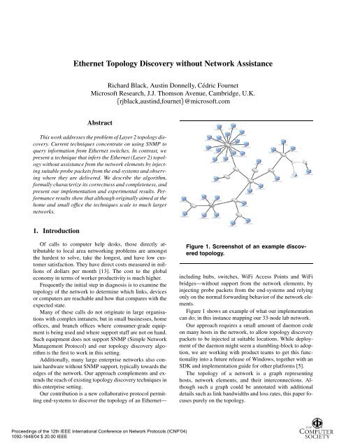
Figure 1. Screenshot of an example discovered
topology.
including hubs, switches, WiFi Access Points and WiFi
bridges—without support from the network elements, by
injecting probe packets from the end-systems and relying
only on the normal forwarding behavior of the network elements.
Figure 1 shows an example of what our implementation
can do; in this instance mapping our 33-node lab network.
Our approach requires a small amount of daemon code
on many hosts in the network, to allow topology discovery
packets to be injected at suitable locations. While deployment
of the daemon might seem a stumbling-block to adoption,
we are working with product teams to get this functionality
into a future release of Windows, together with an
SDK and implementation guide for other platforms [5].
The topology of a network is a graph representing
hosts, network elements, and their interconnections. Although
such a graph could be annotated with additional
details such as link bandwidths and loss rates, this paper focuses
purely on the topology.
Proceedings of the 12th IEEE International Conference on Network Protocols (ICNP’04)
1092-1648/04 $ 20.00 IEEE

Topology discovery can be at a variety of levels, ranging
from Internet-scale mapping efforts to small-scale home
area networks. The techniques applicable to one effort are
not necessarily transferable to others; this paper describes
Ethernet (Layer 2) topology discovery.
Topology discovery should ideally return the simplest
network compatible with all observations. However, the potential
presence of hubs and switches not directly linked to
any hosts significantly complicates our task. Clearly, some
elements cannot be detected by any sequence of packets—
for instance, a switch attached to a single segment is invisible.
More surprisingly, perhaps, it is often possible to infer
the presence of hubs and switches far from any host involved
in the protocol. To clarify these ideas, and gain confidence
in our protocol, we formalize the observable semantics
of networks and show that, in the absence of wireless elements,
our discovery algorithm is correct and complete.
Section 2 covers related work. Section 3 reviews the behavior
of various network elements and defines our terminology
and notations. Section 4 explains the algorithm, and
section 5 describes some limitations, security aspects, and
the extensions to wireless networking. Section 6 considers
the correctness and completeness of the algorithm. Section
7 evaluates its implementation, both on real networks
and in simulation. Section 8 presents our conclusions.
2. Related Work
Recently, there has been much research into Internetscale
mapping or tomography [9, 12, 2]. These tend to be
passive, non-collaborative, IP-layer protocols (although [3]
like us uses active probing). For individual routes in the Internet,
tools such as traceroute and pathchar [7] can be used
to discover link characteristics. Mapping at this level in such
a large environment is far removed from our work; it considers
topology at the IP level and tends to apply to the wide
area and multiple organisations, whereas our work applies
to the local area (a single Ethernet), and a single organisation.
Of course the techniques could be used and combined
in an overall larger picture.
Closer to our problem is that of mapping enterprise or
datacenter networks. In this area commercial products such
as IBM/Tivoli’s NetView and HP’s OpenView are common
[14, 8], along with the more basic Nomad [4] and
OpenNMS [1]. These mappers work by issuing SNMP
queries for router tables (defined in MIB-2) [11], IEEE
802.1D Bridge MIBs [6], and / or RMON-2 MIBs [15].
These MIBs give information for each port on the IP router
or Ethernet switch, including the hosts or network elements
attached to these ports.
These management interfaces have some variation in
their implementation; Lowekamp et al. report needing to
develop work-arounds [10] in their presentation of an efficient
technique for stitching together the partial topologies
resulting from SNMP queries into a consistent whole, using
contradictions to quickly narrow down the possible interconnections
between switches.
Several problems remain with MIB based approaches:
MIBs only contain information on recently active hosts
(since bridges timeout address table entries after around five
minutes); properly secured network elements need the mapper
to supply an appropriate community string (i.e. password)
before allowing access.
Most significantly however, many devices especially in
the application domain of interest do not support SNMP;
indeed, for an ad hoc wireless network there is no device!
We believe that our approach, using a careful analysis of
only the fundamental packet forwarding properties of the
network elements themselves, is new and provides an effective,
end-system-based way to map networks.
3. Terminology
We introduce two new terms: islands and gaps in our
discussion of network topology. However, since our approach
relies on observing and analyzing the standard operational
behavior of the network, we begin with a short summary
of the operation of network elements before we define
those terms. Section 6 gives formal definitions, in terms of
simply-connected graphs and subgraphs.
Hosts, Addresses, and Packets. An Ethernet is a graph
with two kinds of nodes: hosts, with a single link, and network
elements, with multiple links. Ethernet requires that all
redundant links have been eliminated (either through STP
(Spanning Tree Protocol), or by wiring rules); the graph is
therefore a tree, with a single path between any two nodes.
Each host is characterized by its distinct MAC address,
thus a computer with multiple network interfaces is treated
as multiple hosts.
Switches and Hubs. To the reader, it might seem clear
whether a particular element is a switch or a hub, but given
the abuse of terminology used in much marketing literature,
we feel a hard definition is needed.
Switches are devices that can dynamically learn which
addresses are on each port, and filter packets destined to
those addresses accordingly. Concretely, if a switch receives
a packet with source on a given port, then it subsequently
delivers packets for destination to that port only; packets
from that port with destination are dropped. If no
packet from source has been seen, then the switch floods a
packet to that destination to all ports. We do not require that
switches implement the IEEE 802.1D STP, since so many
inexpensive switches do not.
Hubs are stateless devices; they always flood received
packets to all ports except the original incoming port.
Proceedings of the 12th IEEE International Conference on Network Protocols (ICNP’04)
1092-1648/04 $ 20.00 IEEE

Network diagrams (such as in figure 2) in use square
boxes to represent network elements, with an ‘X’ for
switches and an ‘H’ for hubs.
Segments. We use the standard meaning of segment: a
shared media where hosts overhear each others’ transmissions
(e.g. a 10Base2 coax bus or at least one 10BaseT hub).
A segment with at least one host is a shallow segment and
considered to be at the edge of the network; segments with
no hosts are called deep segments. For brevity we sometimes
identify a segment with a host present on the segment.
We classify segments as intermediate if a packet being
put onto the segment may arrive at more than one switch. It
follows that a shallow segment is intermediate if it contains
at least two switches; a deep intermediate segment requires
at least three switches since it has no hosts.
For instance, figure 2 shows a simple network comprising
four hubs and two switches, with eight hosts arranged
in pairs on four segments. The segment containing
is an intermediate segment.
Islands and Gaps. An island consists of one or more shallow
segments of the network, forming a maximal connected
subgraph with no deep segments.
A gap is a portion of a network containing only deep segments;
it therefore connects multiple islands together.
For instance, figure 2 shows a single island; figure 5
shows three islands connected by two gaps (both just a
wire); figures 7 and 8 illustrate more complex gaps, composed
of several deep segments.
Access Points. Wireless APs (Access Points) partially filter
packets: they maintain a table of addresses associated
with their wireless port, and transmit a packet on the wireless
port only if its destination address appears in the association
table (or if it is broadcast or multicast). An AP
does not forward a packet to an unknown destination from
its wired to its wireless interface. Packets arriving from the
wireless side with a destination address that does not appear
in the association table are bridged to the fixed side of
the AP. We say a host is behind an AP if it is connected to
the AP’s wireless side.
Note that a consequence of association is that wireless
clients of an AP must send packets with a source address
which has previously associated: this precludes the forging
of source addresses.
Wireless Bridges. Wireless bridges (such as the Linksys
WET11) are also devices with one wired and one wireless
port: they are designed to permit one or more wired computers
to associate indirectly to a wireless access point. We
say that the wired computers are behind the bridge.
Wireless bridges require care during discovery because
hosts can appear to be connected to a fixed network when
actually there is a point-to-point wireless link between them
and other portion(s) of the network.
We consider bridges which operate in one of two modes.
In clone mode, the bridge notes the first source MAC address
it receives on its fixed side, and associates to the AP
using that address. This only allows a single host behind the
bridge, however it provides true Layer 2 bridging semantics.
In proxy mode, the bridge associates with the AP using
the bridge’s own address. It performs proxy-ARP for
the IP addresses on the wired side, building a table of IP
and MAC addresses; when packets arrive on the wireless
side, the bridge rewrites them to have the correct destination
MAC address (rather than its own), and sends them
out on the fixed side. Packets from the fixed side have their
source MAC address rewritten to be the bridge’s own, since
this is the address associated with the AP. This allows multiple
IP hosts to operate behind the bridge, but does not provide
true Layer 2 connectivity.
4. Algorithm
At a very high level the technique is based on two simple
properties: (1) hosts on the same segment can be detected
since in promiscuous mode each can see all the traffic
of the others, and (2) a packet with a particular source address
entering a switch on one port will prevent the switch
from sending packets with that destination address to any
other port.
Assumptions. In our implementation we use a distinguished
host Å, themapper, that acts as a central controlling
entity for the algorithm. We also assume that most hosts
in the network run a daemon that can inject topology packets
and record received packets (using promiscuous mode);
section 5 relaxes our assumption for some hosts.
A preliminary protocol permits us to discover all hosts
running daemons, and establish a control RPC connection
to them. The RPC interface permits Å to request the transmission
of a packet and query which packets have been observed.
The mapper determines the sequence, addresses, and injection
points for packet transmissions, and how such transmissions
are interleaved with queries. The RPC protocol is
fairly standard so hereinafter we simply assume that the algorithm
directly controls all hosts. Throughout the discussion
we assume that no packet loss occurs; the real implementation
uses either acknowledgements (where a packet
always arrives somewhere) or repetition (where a test packet
may be validly not delivered anywhere) but we elide these
details for clarity and space; the technique used at each
stage is obvious from the discussion below.
For our notation we let ÈÉ range over
host MAC addresses. In addition, we sometimes rely on addresses
Ä not attributed to any host on the network but
instead allocated from a private range assigned for our technique.
Proceedings of the 12th IEEE International Conference on Network Protocols (ICNP’04)
1092-1648/04 $ 20.00 IEEE

We use the notation to mean that host
sends an Ethernet packet with source address and destination
address . Note that in standard Ethernet is at liberty
to fake the source address, indeed we exploit this in
our algorithm; because such addresses are from a private
range always different from real addresses, normal traffic is
not disturbed. Topology discovery packets also use a distinct
Ethernet Type field to further prevent interference.
In description we may distinguish training and probe
packets: training packets cause a switch to learn a particular
source address, whereas probe packets test whether a
switch has learnt a trained address. Of course on the wire
there is no difference between them.
Outline. Mapping proceeds by execution and analysis of
a number of phases. We initially explain the wired algorithm,
and subsequently explain the extensions for wireless
elements and uncooperative hosts in section 5. We also ensure
that all switches know the real addresses of all hosts at
the beginning of the mapping, using ordinary broadcasts.
The first phase discovers the shallow segments of the network
by the use of promiscuous mode. Shallow intermediate
segments can also be deduced from the promiscuous
mode information obtained.
The second phase discovers switches attached to at least
one shallow segment, plus the shallow segments they are attached
to, and fully determines all islands (defined in section
3 above). In the usual case there are no shallow intermediate
segments, hence each island consists of a single switch
that attaches shallow segments.
The third phase discovers the segment or switch at the
edge of each island where it connects to its adjoining gaps.
Finally, the fourth phase discovers the structure of the gaps
that interconnect the islands.
Phase 1: Segment Detection. We select an arbitrary host,
named the collector, and set all hosts in promiscuous mode.
Each other host sends a probe packet to the collector. The
collector also sends a probe packet using a special segmentlocal
destination address Ä (described below) so that any
hosts sharing its segment may see it. For each host, the sees
set consists of the source addresses for all received probe
packets, plus the host’s own address.
From these sets, we determine shallow segments and
their interconnection, as follows. Two hosts belong to the
same segment if they have the same sees set. Further, we
sort shallow segments into a tree, the segment tree, by placing
a segment above another when hosts in the parent segment
see the probes sent from the child segment. Hence, the
collector’s segment is at the root of the tree, and branches
appear when multiple segments are attached towards the
collector.
Consider the network in figure 2, consisting of eight
hosts  connected to several hubs joined by
switches, all of which have engaged promiscuous mode.
H
A B
H
GJ
H
CD
flow of
packets
H
EF
Segment Tree:
segment
A, B
segment
C, D
segment
E, F
segment
G, J
Figure 2. Segment detection.
Let be the collector. The leaves and only see
; similarly, and  only see Â. Further in,
and see , while and see all eight
hosts (since is the collector). Hosts are in the same segment
if they have identical sees sets, so in our case the shallow
segments are , , ,and Â.
For the subsequent phases, we select one host to represent
each shallow segment; this host is called the segment
leader. Other hosts play no further part. In our example we
select , , and .
Phase 2: Switches. In this phase, we detect any switch
shared between multiple shallow segments by observing
when a switch trained by (the leader of) one segment
changes behavior when observed by (the leader of) another
segment.
We first establish a technique to teach an address to exactly
the switches of a given segment—a host cannot do so
by sending a packet to its own address, since such packets
are internally looped-back.
The IEEE defines in the 802.1D standard a range of addresses
which must not be propagated by switches; the first
of these is used by the STP. We cannot use one of these addresses
however, since consumer switches flood these packets
precisely in order to appear transparent to STP.
Instead the host (say ) sends a packet Ä
where Ä is a fresh address and is the address of some
other host. 1 Whilst knowledge of Ä may leak to many
switches in the network, at least the switches on ’s segment
are trained that Ä is on ’s segment. Host can now
send to destination Ä, with the guarantee that no switches
will forward the packet. Note that Ä is specific to ; each
host will need to set up its own fresh address Ä.
Having established the ability to send packets to a single
segment we can explain a simple example of training to detect
switches and discriminate between the two networks in
figure 3 by sending three packets. First, Ä. Second,
Ä. Third . If the second packet
reaches the same switch as the first packet (figure 3(a)), then
1 It is more efficient to use another host on ’s segment, but any other
host or even broadcast will do.
Proceedings of the 12th IEEE International Conference on Network Protocols (ICNP’04)
1092-1648/04 $ 20.00 IEEE

A B A B
H
A B
H
H
C D
H
(a)
(b)
G J
E F
Figure 3. Training to separate two switches.
Figure 4. Probe flow after training A;C;E;G.
the third packet will be forwarded by the switch to host .
If and are attached to different switches (figure 3(b)),
the third packet will not reach host .
We expand the description of our general technique in
two stages for clarity. First, suppose that there are no intermediate
segments in the network. We pick one fresh address,
, which will be repeatedly trained. Each segment
leader Ë sends a training packet Ë Ä. Ifthereare
multiple segment leaders connected to a single switch then
will be repeatedly trained so that for each switch the last
segment leader to send the training packet will be the owner
of address on its switch. Note that each switch will have
a different view as to the location of the host .
We then cause each segment leader to send a probe
packet Ë Ë , and observe which segment leaders
receive the probes. Any switch with a segment leader
attached has one segment leader which was the last to train
the switch with the address ; that leader will receive probe
packets sent by other attached segment leaders. We say that
this host gathers the probes from the other segment leaders
on the same switch; the gathered segments and the gathering
segment are attached to the same switch. Any segments
remaining unaccounted for (neither gathered nor a gatherer)
are each connected to a separate switch by themselves (they
train their local switch and probe it, but the switch correctly
drops the probe packet so it is never received).
Now relax the restriction and consider intermediate segments.
As shown by ’s segment in figure 2, a segment can
be attached to several switches; a training packet sent by the
leader of an intermediate segment trains multiple switches.
If the leader of an intermediate segment was the last host
to train more than one switch then it would be a point of
confluence for the probe messages, and could erroneously
gather the segments of multiple switches and believe them
to be attached to the same switch. As an example, consider
figure 2 and suppose that was the collector. If was also
to train last, it would gather from , and and the two
switches of the network would be indistinguishable.
We solve this by having the segment leaders train in preorder
when performing a depth-first walk of the segment
tree (starting from the collector). This means that probes
sent to now propagate away from the collector towards
the leaves of the tree, guaranteeing that there is no point of
confluence.
For the running example of figure 2 the segment leaders
would train in the order: . The probes would
therefore flow as shown in figure 4, yielding the following
gathers sets: and both gather nothing, gathers ,
and gathers . The switch connectivity is known.
There is one further detail: the existence of intermediate
segments can mean that probe packets to can traverse
more than one switch across the network. If host were
to train before host in figure 2, the probe from would
travel the whole way to . Such probes are easily handled
because they come from a host which is neither a peer not a
direct parent of the gatherer in the segment tree.
At this point in the algorithm we have linked shallow
segments to their switches, and if intermediate shallow segments
are present then they chain together the multiple
switches they connect, forming islands in which the complete
topology is known. Switches not attached to intermediate
shallow segments form trivial one-switch islands
comprised of the switch together with its (non-intermediate)
shallow segments. What remains to be investigated are the
deep segments and the switches interconnecting the islands.
Phase 3: Island Edges. From the segment tree, we can
easily detect parent- and child-segments on different islands,
hence the existence of a gap to analyze, but we first
need to know whether the paths to each of these children
attach to the parent through distinct switches, or whether
these paths share points of attachment to the parent. In brief,
we need to identify the switches at the edge of each island.
Figure 5 shows a topology with three islands and two
gaps. Host Å is collector, at the root of the segment tree.
The figure also shows the segment tree resulting from running
the first phase of the algorithm.
The segment of interest is the segment of host which
has four direct children , , and in the segment tree,
representing the three islands. We chose this network because
it shows both an island (number 1) connected via a
switchdiscoveredinPhase2,andanislandconnectedvia
an additional switch.
Our algorithm analyzes each cross-island parent-child
connectivity in turn. There are two possible cases to consider:
(1) if the parent segment has no switches below it in
the segment tree, then we create a new one representing the
switch through which the child’s island attaches to the parent’s
island. We know this switch must exist because if it
Proceedings of the 12th IEEE International Conference on Network Protocols (ICNP’04)
1092-1648/04 $ 20.00 IEEE

island 1
island 0
B
A
M
H
switch S
island 2
H
switch T
segment
B
segment
C
segment
M
segment
A
segment
D
segment
F
CD
E
F
G
segment
E
segment
G
Figure 5. Example network with three islands, and the resulting segment tree after Phase 2.
did not then we would have discovered a single, larger, island
rather than the two we actually discovered. Alternatively,
(2) the parent segment has one or more switches below
it in the segment tree. We thus need to discover which
one of these switches connects the child’s island to the parent’s
island. We test each candidate switch as follows: we
send a probe packet from the child segment to a host below
the switch under test; if the probe packet is not seen
on the parent segment then the child segment must be below
the switch under test, and so the child’s island attaches
to the parent’s island via this switch. If the child’s island is
not connected via any of the candidate switches then we infer
the existence of a new switch, just as in case (1) above.
In the example, a packet sent from host in island 1 to
host in island 0 is not visible at host , therefore we know
that ’s segment (hence island 1) is connected via the same
switch as host . In contrast, a packet sent from host in
island 2 to host is visible at host allowing us to infer
the existence of switch Ë.
To complete the discovery of cross-island connectivity,
we determine the switch at the child segment on the edge of
the island; fortunately this is deterministic and easy. If the
child segment has a parent switch, then it is the edge of the
island (all the other segments on that switch are also children
of the same parent and can be removed from consideration).
If the child segment has no parent switch, then we
infer the existence of an additional switch.
In the example, hosts and share a parent switch, so
that switch is at the edge of island 1; host has no such
parent switch, so we can infer the existence of switch Ì at
the edge of island 2. (Recall that switches Ë and Ì must be
distinct because and are in different islands; if they had
been a single switch, would have gathered in Phase 2.)
At the end of this phase, we have discovered all hosts and
switches attached to shallow segments; further, for each remaining
gap, we have identified the islands connected by
that gap, and the corresponding switches at the edge of the
gap. For each gap, we now select one host per island to train
and probe the gap via its edge switch. We call these hosts
switch leaders.
Phase 4: Discovering Gaps. In order to explore any remaining
gap, we first set up a simple test, then describe a
recursive discovery algorithm.
Path Crossing Test. Our test combines both training and
probing with a fresh address, say ; it involves four switch
leaders, say È and É, at the edge of the gap.
The purpose of the test is to determine how the path from
to intersects the path from È to É. It is especially useful
for exploring deep segments because the intersection between
the two paths need not be close to any of the hosts involved
in the test. It goes sequentially, as follows:
1. sends a training packet to ( ).
2. È sends a training packet to É (È É).
3. sends a probe packet to ( ) and both
and È report whether they receive the probe or not.
The test and its results are depicted in figure 6. We now interpret
each of the three possible results, and also define notations
used in this phase.
Only È observes the probe: Since does not observe
the probe, some switch on the path from to has been
trained by the packet È É. That is, there is a switch
that is both on the path from to andonasegmenton
the path from È to É. We say that the two paths cross at that
switch, and write È É ¢.
Only observes the probe: Since È does not observe
the probe, conversely, we know that the switches on the segments
on the path from to (seeing the probe message)
and the switches on the segments on the path from È to É
(trained to forward to È ) are disjoint. Moreover, since
and È still have to be connected, this connection necessarily
goes through one of the former switches and one of the
latter switches, and the deep segments between these two
switches separate the network with , on one side and
È , É on the other side. We say that the two paths are disjoint,
and write È É .
Both and È observe the probe: This third result reveals
the presence of a deep hub that duplicates the probe
packet sent to . Precisely, there is a switch on a segment
of the path from È to É that is also on a segment of the path
Proceedings of the 12th IEEE International Conference on Network Protocols (ICNP’04)
1092-1648/04 $ 20.00 IEEE

Q
island 0
island 1
island 2
D
A
P
A
1
X
B
Q
B
?
A
P
P
2 X Q
B
Q
A
P
B
3 B X
Figure 6. The test ÈÉ and its results.
from to , but that is not directly on that second path. We
say that the two paths are hubbed, and write È É H.
The test can be used with È É, with packet two becoming
È Ä, yielding three possible results with
similar interpretations. (È É is not defined, but for uniformity
it is convenient to extend our definition and let
È É .)
Our “path-crossing” test has useful equational properties,
which can be used to reduce the number of tests actually
performed during gap discovery. For instance, we have
ÈÉ È É ÉÈ ,andÈ É if
and only if ÈÉ . Besides, series of tests È É
can often be combined to reuse the same training- or probepackets.
Recursive Gap Discovery. Recall that at the end of the third
phase we have detected some number of gaps in the network,
each of which bordered by switches, each switch having
a host (the switch leader) on an attached segment. Starting
from these switches, we recursively use the path crossing
test to split each gap into smaller gaps until we are left
with wires. (This section explains how to split gaps, but the
precise tracking of the sub-gaps is deferred till section 6.)
As a first step, we check whether any switch on the edge
of the gap has more than one deep segment attached to it, as
this allows us to break the gap at such a switch. This is done
by choosing each switch leader in turn to be the host È ,
and testing È È for all remaining hosts as and s.
Whenever there exist some and with È È H
or È È ¢, one can split the current gap into several
gaps with fewer border switches: one of these gaps has
switches for (at least) and È but not for , another has
switches for and È but not for . We iterate this process
until all such gaps are split.
H
H
B
Q
D
E
F
E
gap
Figure 7. A network with a three-switch gap.
As a simple example, consider the three-switch network
shown in figure 7, and the problem of determining how
those switches are connected. By the end of Phase 3, we
know they are in three separate islands, and all border the
same gap. Suppose we select as È ; without loss of generality
is and is . The result of is , so
does not split the gap; by symmetry the same holds if we select
as È .However,whenwepick as È we find that
is ¢, splitting the gap into two gaps each of two
switches. Such gaps are trivially represented by a wire, and
hence the switches are connected in the order -- .
In the next step, we observe that in the case of a gap
whose segment closest to some host È is an intermediate
segment, then a packet on a path from È to a switch leader
behind one of the switches on such a segment is sufficient
to train a switch connecting some other part of the gap attached
to the same segment. We can thus apply È É recursively,
with the path ÈÉtouching the edge of the gap under
evaluation as long as there is some segment on the edge
of the gap which is an intermediate segment.
As an example, refer to figure 5, assume hosts and
are inactive, and consider the gap bordered by , Å, , .
Packets suffice to train switch Ì , so we can
proceed as if were active, and recursively fill the gap bordered
by , Å, and (virtually) . Symmetrically, packets
Å suffice to train switch Ë,asif were present.
Finally we may reach a stage where every edge of some
gap is represented by a switch with a single wire leaving
that switch into the gap attached to a single other switch.
At this point we must apply the general form of È É.
We chose È and É such that ÈÉ crosses the gap and then
we group the remaining switch leaders into classes and subclasses
based on the evaluation of È É. Once this is
done we can order the classes along the line ÈÉby sorting
with ÈÉ. This gives us the number of switches along
the line ÈÉwhich have points of attachment, the number of
points of attachment to each such switch, and the classes of
switch leaders attached to each switch. (See section 6 and
figure 9 for example networks.)
We proceed to analyse the gap by recursion; choosing a
new É inside each such class and repeatedly dividing the remaining
switch leaders into classes and subclasses, and ordering
the classes. Depending on the topology this may be
quite expensive, but since at least one switch leader (the one
F
Proceedings of the 12th IEEE International Conference on Network Protocols (ICNP’04)
1092-1648/04 $ 20.00 IEEE

H
Figure 8. Two indistinguishable 3-stars.
chosen as É) is removed from the switch leaders under consideration,
it will eventually terminate with the topology of
the network (under observational equivalence).
5. Discussion
Limitations. There are certain configurations of networking
equipment which we cannot detect. The most obvious is
a dead branch such as a hub or switch with no hosts, hanging
as a leaf from the network. These have no operational
effect, and so are undetectable in our setting.
Some live equipment is also undetectable. A segment
(apparently) connecting only two devices may be either a
piece of wire or an arbitrary number of linked hubs; similarly,
any collection of hubs on the same segment are indistinguishable
from a single, larger, hub. Likewise, a switch
connecting exactly two deep segments forwards any packet
it receives on one port to the other port; it has no effect on
packet flow, and is indistinguishable from a wire.
Finally, deep hub stars are indistinguishable from a single
switch connecting the arms of the star; again none of
the equipment has hosts directly connected. Figure 8 shows
two indistinguishable 3-stars, although clearly this generalises
to an Ò-star for Ò½.
In all cases, we apply Occam’s Razor and infer the simplest
network which satisfies the observable properties.
A limitation of another sort comes from switches running
with 802.1x port-based access control enabled. Such
switches prevent hosts connected to them from sending
packets with unauthenticated source address. This stops us
from training their switches, and thus we cannot determine
which hosts attach to them. However, such switches are
high-end products and also implement a remote management
interface, allowing their topology to be discovered
through more traditional schemes.
Wireless. So far we have described wired hosts on a wired
network; we now explain how wireless hosts and segments
fit into the technique.
First, recall from section 4 that we begin by finding all
the hosts in the network supporting the daemon. At this
original stage, hosts attached to a wireless NIC report the
BSSID of the AP that they are associated with.
While in theory there is nothing preventing a wireless
host from enabling promiscuous mode, in practice this requires
firmware support on the device and driver support
in the OS. In our experience, enabling promiscuous mode
on a wireless NIC does not work reliably, so we do not depend
on this behavior. Instead we use BSSID equality to detect
wireless hosts on the same segment.
At the original stage hosts also supply their real MAC address
in the body of the packet. This allows us to detect if a
wireless bridge has rewritten the source address in the Ethernet
header. We group hosts with equal changed addresses
(which is the address of the bridge attaching them to the network)
and use recursion to map the portion of the network
on the wired side of the bridge. 2
We locate APs and bridges in Phase 2 by electing a leader
for the AP or bridge. The leaders send a probe packet to address
, and we note where it is gathered, just like any other
host. The difference is that hosts behind an AP cannot take
part in training switches, so their probes may be gathered
some distance from their actual location. 3
Uncooperative hosts. While it is desirable to have all
hosts run the daemon code, mapping is possible without
having the cooperation of all hosts—although obviously the
accuracy of the topology may be affected. Any host not
running a daemon but having an IP stack (e.g. a network
printer) can be located in the network in a similar way to the
locating of APs and bridges: the mapper can send a thirdparty
ARP request for the address to the host’s IP address.
A third-party ARP request is one whose ARP-layer
source address is not the sender’s. In our case the mapper
sets the ARP source address to be , which makes the IP
host send an ARP response to , so it can be gathered in the
normal fashion. The mapper could collect the list of IP addresses
to be probed passively, by continuously monitoring
traffic on the network—the list need not be manually configured.
Security Aspects. The daemons send and receive packets
on behalf of the mapper. To mitigate security concerns,
daemons only send and record topology traffic packets, and
send packets only from either our reserved topology address
range or their real address. This prevents any impact on the
routing of normal packets. In addition, the daemons enforce
a rate limit on transmission to prevent their being used in
an amplification attack. As in any collaborative scheme, the
correctness depends on the correct behavior of the contributors.
2 It may be that the mapper is behind a wireless bridge; this is detected
by the mapper’s address changing. Whilst this adds a little complexity
to the implementation it doesn’t much affect the algorithm; each wired
region is mapped independently.
3 This rarely causes any ambiguity since wireless segments cannot be
intermediate segments.
Proceedings of the 12th IEEE International Conference on Network Protocols (ICNP’04)
1092-1648/04 $ 20.00 IEEE

6. Correctness and Completeness
In this section, we give a formal account of our algorithm.
Throughout, we assume there is no wireless element
or uncooperative host. Due to space constraints, we only
give a sketch of the proofs.
Basic Definitions and Tests. We first recall our definitions,
in terms of graphs. A network is a simply-connected,
finite graph whose nodes are switches, hubs, and distinct
hosts , ,..., È , É,..., Ì ,....Hostshaveasinglelink.
We write for the unordered pair of hosts and .
An Ò-segment is a maximal, simply-connected subgraph
of linked hubs attached to Ò (distinct, otherwisedisconnected)
hosts and switches. The segment is shallow
if it is attached to at least one host, deep otherwise. For instance,
a ¾-segment is typically just a link, but may also be
two links attached by a hub.
An island is a maximal simply-connected subgraph consisting
of shallow segments; An Ñ-gap is a simplyconnected
union of deep segments that connect Ñ (distinct)
border switches.
Next, we provide lemmas that formally relate the results
of tests performed on networks to their actual topology. All
tests assume that all switches are initially trained for all host
addresses; this can be enforced by sending for
all hosts and .
Lemma 1 (Seeing Packets) Let be the set of hosts
on segments that connect to . This set is observable.
The set contains at least and . For ,
we have È ¾ if and only if host È observes packets
(or equivalently ). For ,
we observe È ¾ using local training, as detailed in
section 4.
For a fixed host Ì , the collector, we write Ø when
¾ Ì . The relation Ø is a preorder with smallest element
Ì . When convenient, we also use the associated equivalence
Ø (when Ø and Ø ), strict preorder
Ø (when Ø and Ø ), and covering relation
Ø (when Ø and Ø Ø implies
Ø or Ø ). By definition, all these relations are
also observable.
Lemma 2 (Path Crossing) For all hosts È É with
, letÈ É ¾ ¢ H be such that
¯ È É when there exist two switches separating
, on one side from È , É on the other side.
¯ È É ¢ when there is a switch on a segment of
the path from È to É that is on the path from to .
¯ È É H when there is a switch on a segment of
the path from È to É that is also on a segment of the
path from to but not directly on that path.
The result of È É is observable.
Network Equivalence. We let observational equivalence,
written , relate two networks when they have the same
hosts and, starting from a state where all switches are clear,
for any series of packets sent from these hosts, all hosts observe
the same packets.
This equivalence captures our intuition of indistinguishability
of networks, from the viewpoint of its hosts. However,
it does not provide an effective decision procedure. To this
end, we now give a characterization of in terms of the local
network topology. In essence, our theorem bounds what
can ever be observed without network assistance. This enables
us to confirm that our discovery algorithm is complete:
under our hypotheses, its precision cannot be improved.
Theorem 1 (Completeness) Observational equivalence is
also the finest equivalence preserved by:
R1. Substitution between Ò-segments.
R2. Addition and deletion of dead branches: for any network
N, we have N H N and N ¢ N.
R3. Addition and deletion of redundant switches with two
links: for any networks N, N ¼ , we have N¢ ¢ ¢N ¼
N¢ ¢N ¼ .
R4. Addition and deletion of deep hub stars: for any networks
N½N , we have H´ ¢ ¢N µ ½
¢´ ¢N µ ½ .
(where ¢N and HN stands for networks N½N Ð attached
to ¢ and H, respectively.) Informally, the rules R1–R4 list
parts of the network topology that are not observable: attached
hubs (R1), ends of the network with no hosts (R2);
switches attaching two deep segments (R3); and hubs symmetrically
attaching deep ¾-segments, as depicted in figure
8 (R4). The theorem states that this list is actually complete.
The normal form of a network is obtained by repeatedly
applying these rules from left to right, and replacing any Ò-
segment by a single hub attaching Ò wires (or just a wire for
Ò ¾). Since each application deletes elements, we obtain
the smallest network in its equivalence class.
An abstract discovery algorithm performs a finite series
of tests for each given network and returns its normal form.
Proof sketch Let be the finest equivalence preserved
by rules R1–R4. To prove that N N ¼ implies N N ¼ ,
it suffices to check that each of the equivalence cases in
the theorem is an observational equivalence. These different
networks can’t be separated by any series of packets because:
R1. Hubs on a segment don’t filter messages.
R2. No message ever arrives from a dead branch.
R3. As an invariant, the state of the two left- and rightswitches
are the same on both sides of the equivalence;
Proceedings of the 12th IEEE International Conference on Network Protocols (ICNP’04)
1092-1648/04 $ 20.00 IEEE

if the left switch routes to the right, or the right switch
routes to the left, then so does the middle switch.
R4. As an invariant, the outer switches have the same state
on both sides of the equivalence, and the states of each
inner switch is obtained from the state of the central
switch by routing outward the addresses routed towards
that branch by the central switch and routing inward
the addresses routed towards any other branch by
the central switch.
Conversely, to prove that N N ¼ implies N N ¼ ,we
rely on the existence of a correct abstract algorithm (Theorem
2): since the algorithm yields the -normal form of
the network, and since it only depends on the result of observable
tests, -equivalent networks yield identical normal
forms. £
An Abstract Algorithm. We now specify our algorithm,
omitting the details, data structures, and optimizations of
our implementation. Our discovery strategy relies on fewer
tests than those we implemented. In the discussion, we implicitly
refer to the normal form of the network, thereby excluding
occurrences of the right-hand-sides of rules R1–R4.
Determine the islands and their contents (Phases 1 and 2).
Choose a host Ì and observe Ø ,then
1. Find all shallow segments, as the equivalence classes
of Ø . Retain a single host on each shallow segment.
2. Find all switches attaching shallow segments. We distinguish
two cases for these switches: (I) the switch attaches
Ò ·½segments ½ Ò with Ø
for ½ Ò, or (B) the switch attaches Ò segments
½ Ò and also connects to on some other island
(through deep segments), with Ø for ½Ò.
Phase 2 proceeds as follows:
a) Every sends Ä, in increasing order: if
Ø ,then sends its message before .Asaresult,
every shallow switch is trained and, in both cases
(I) and (B), the switch is trained towards the that
sent Ä last.
b) Every sends , in any order. The result
of the test consists of sets Ë containing the source
for each packet observed at .
We find a switch attaching shallow segments for each
non-empty set Ë : either there exists Ø for
some ¾ Ë , and we have a (I)-switch attaching
¾ Ë Ø , or we have a (B)-switch
attaching Ë .
Determine the switches attaching islands to gaps (Phase 3).
We write when Ø and and belong
to different islands: and ’s islands are then connected
by a gap via switches attached to and , respectively.
Hence, the relation yields the branches of a tree of islands
rooted at Ì .If and ¼
for two distinct
and ¼ on the same island, then and ¼ are attached to
a previously-found (B) switch connecting ’s island. Otherwise,
is attached to a newly-found switch connecting
’s island.
On ’s island, we may need additional tests to find the
switch attaching and connecting each island with a
such that . For each with Ø with a
previously-found switch attached to and connecting ,if
¾ then is also connected to that switch. Otherwise,
we have found a new switch (and will consider
for any remaining island connected to ).
To every such identified switch attached to corresponds
a Ñ-gap, with Ñ ½ additional switches, one for
each island with s such that .
Determine every remaining Ñ-gap, by induction on Ñ
(Phase 4). The input is a set Ë of Ñ unordered pairs ¼
representing distinct switches that can be trained towards
by sending ¼
without affecting the rest of the
gap. To begin with, Ë contains a pair for each border
switch, for some host linked to the switch.
In preparation for the inductive cases, we define an auxiliary
operation on sets of switches: to add a switch represented
by ÈÈ ¼
to some set Ë ¼ , written Ë ¼ · ÈÈ ¼ ,firstdetect
whether the switch ÈÈ ¼
is already represented by any
¼ ¾ Ë ¼ ,usingthetestÈÈ ¼ ¼ ¢, then merge these
two switches and their connections, otherwise add a distinct
switch ¼ to Ë ¼ .
When Ñ ½, do nothing. When Ñ ¾, attach the two
switches by a wire. When Ѿ:
1. Select ÈÈ ¼ ÉÉ ¼ ¾ Ë and partition Ë ÒÈÈ ¼ ÉÉ ¼ as
follows: ¼ and ¼ are in the same subclass when
¼ È É ¼ ; ¼ and ¼ are in the same class
when ¼ È É ¼
¾ H.
Each class corresponds to a network attached to a
switch on a segment from ÈÈ ¼
to ÉÉ ¼ . When a class
contains several subclasses, each subclass corresponds
to one or several networks attached to a distinct switch,
with the class switch and all the subclass switches attached
by a hub.
We distinguish two kind of inductive cases, for
ÈÈ ¼ ÉÉ ¼ and ÈÈ ¼ ÉÉ ¼ . In both cases, a set Ë ¼
collects the switches bordering the remaining gap after
analysing all classes and subclasses; at the state of the
analysis, Ë ¼ contains ÈÈ ¼ and ÉÉ ¼ (when ÉÉ ¼ ÈÈ ¼ ).
After analysing all classes, if Ë ¼
is smaller than Ë, recursively
fill Ë ¼ .
Each class is analyzed as follows:
a) If has several subclasses ½ Ò , then
for each subclass , select ¼
¾ Ò ,fill
· È, and keep the resulting switch.
Proceedings of the 12th IEEE International Conference on Network Protocols (ICNP’04)
1092-1648/04 $ 20.00 IEEE

A
B
A
B
A
B
H
H
H
H
P
Q
P
Q
P
Q
Figure 9. Examples of 4-gaps with deep switches and hubs.
If ÈÈ ¼
ÉÉ ¼ , attach these Ò kept switches to
ÈÈ ¼ by a hub (and do not add anything to Ë ¼ ).
If ÈÈ ¼ ÉÉ ¼ , select ¼ ¾ ½ and ¼ ¾ ¾ ,
attach the switch ¼
and the Ò resulting switches
by a hub, and add ¼ to Ë ¼ .
b) If is a single subclass, fill · ÈÉ ¼ . In the filled
sub-gap, if the switch ÈÉ ¼
is represented by some
¼ with ¼ and ¼ in , add ¼ to Ë ¼ .Otherwise,
since we cannot have three switches in a line,
the switch behind ÈÉ ¼
is represented by some ¼
with ¼ and ¼ in . Add ¼ to Ë ¼ .
We do not progress in only two situations:
i. ÈÈ ¼ ÉÉ ¼ and Ë ÒÈÈ ¼ is a subclass.
ii. ÈÈ ¼ ÉÉ ¼ , ¼ ,andÈÉ ¼ ¼ .
2. Finally, when there is no progress for any choice of
ÈÈ ¼ ÉÉ ¼
¾ Ë, attach the remaining switches in Ë using
an extra switch with Ñ links. £
As an example of inductive cases in the algorithm, consider
the three -gaps of figure 9, with border switches
, , È ,and É. All border switches are linked to an
inner switch, so any splitting with a single switch (say
È ) yields a single subclass containing all other switches
( É). To make progress, we consider splits using
two distinct switches.
In the leftmost gap, È É H, and the split according
to È É yields a class with two subclasses, .
For each subclass, we fill a ¾-gap, È and È,
find inner switches hubbed to a third switch represented by
ÈÉ, and finally fill Ë ¼
È É in a similar way. We
obtain the exact topology of the network.
In the central gap, È É and we have a single
subclass . We fill the sub-gaps È É
and È É and, since these hub-stars are observed as
switch-stars, obtain the topology of the (equivalent) rightmost
network.
Theorem 2 (Correctness) The discovery algorithm finds
the normal form of any network.
Proof sketch In this final case, by 1(b)i we have
È È ¼ for all distinct ¼ , ¼ , ÈÈ ¼ ¾ Ë, soall
switches are connected by a single wire to some other inner
switch in the gap. If Ñ ¿, rules (R3) and (R4) ensure
that we have a single, central inner switch. If Ñ ¿, assume
some of these inner switches are not the same, that is,
there exist ¼ and ¼ connected by three or more segments
of the form ¼ ¢ ¢ ¡¡¡ ¢ ¢ ¼ .Ifthereexists
ÈÈ ¼ linked to ¼ ’s inner switch and ÉÉ ¼ linked
anywhere else on that path, then ÉÈ ¢ contradicting
1(b)ii. By rule (R3) and symmetry, all inner switches are
thus distinct and attached to a hub. By rule (R4), they cannot
all be connected to a single central hub, so there exist distinct
¼ ÈÈ ¼ on some hub and ¼ ÉÉ ¼ on some other
hub linked by (at least) one switch, with ÈÉ ¢ contradicting
1(b)ii. £
7. Experimental Evaluation
In addition to developing and formalizing the algorithm
itself, we also created an implementation, consisting of
about 4,000 lines of code for the mapper and about 500 for
the daemon, which we used to validate our model against a
real network. A screenshot of our code run on our lab test
network was presented in figure 1.
As well as deploying on our internal networks, we also
purchased one of every home networking switch on offer at
our local store. Some of these experiments informed more
practical considerations: our implementation begins with a
special packet sequence to detect switches based on the
Conexant CX84200; this chip sometimes reflects packets
out the port they went in on which is disastrous to the normal
operation of a network, and too confusing for our algorithm
to deal with. 4 Another surprise was that while inexpensive
home networking switches learn new Ethernet addresses
immediately, enterprise-class switches can take up
to 150 ms. Our implementation therefore delays between
4 The Linksys BEFW11S4 has a similar problem, but we have yet to
find a way to detect it.
Proceedings of the 12th IEEE International Conference on Network Protocols (ICNP’04)
1092-1648/04 $ 20.00 IEEE

sending a training packet and the probe packets which test
the training.
In our implementation we created an abstraction above
the raw Ethernet socket interface, which permits us to run
unmodified mapper and daemons on a simulated network.
This allows testing of our implementation on many different
topologies to exercise the various code paths.
Experimental results. We instrumented the simulator to
record the number of packets injected into the network (including
the RPC traffic from the mapper to the daemons).
We also put together real network topologies to measure
elapsed times.
The table below shows the costs for a small selection
of networks, expressed both as a number of packets (taken
from the simulator results), and the (average) elapsed time
when run on a real network.
Topology pkts secs
(switch A) 6 1.10
(switch A B) 32 2.14
(switch A (switch B)) 38 2.13
(switch A (AP B (bridge C))) 37 3.30
(switch A B (switch C D)) 69 2.61
(switch A B (hub C D (switch E F))) 87 2.64
Three-switch problem (figure 7) 92 3.38
Figure 5 149 4.46
The time is always greater than one second because this is
the length of the host discovery period; time after this initial
second is spent probing the network topology and is dominated
by the many delays of 150 ms in case there are enterprise
switches present.
Although the 150 ms delays are the dominant factor in
the cost of the algorithm we can give complexity information
for the phases. The first phase is linear in the number of
hosts. The second phase is linear in the number of switches.
The third phase is Ç´ ¾ µ where is the number of islands
and is the largest number of gaps attached to any one island.
The fourth phase is more difficult to analyse, but our
experience is that the numbers involved are tiny even in very
large corporate networks.
8. Conclusions
We showed how the hosts on the edges of an Ethernet
can cooperate to discover the topology of the network connecting
them. Not only can the technique map portions of
the network near hosts, but the path crossing test permits the
discovery of network components far from any host.
We do not require any intelligence in the network elements
being discovered, and so our work complements
previous approaches to topology discovery which rely on
querying switch and router MIBs via SNMP or other management
protocols. Because we infer topology from the behavior
of the network, a minor limitation is that elements
which do not influence the behavior are not discoverable by
our technique.
Formally, we specified our algorithm for a wired network,
and showed that it always detects the simplest network
that is observationally equivalent to the actual network.
Experimentally, we presented performance data from
simulations, as well as timings from a real implementation
deployed over 33 machines in our lab.
References
[1] Tarus Balog. OpenNMS. SNMP walker and network
manager, 2004, Available online at
http://www.opennms.org/.
[2] Yigal Bejerano and Rajeev Rastogi. Robust Monitoring of
Link Delays and Faults in IP Networks. In Proceedings of
INFOCOM 2003, April 2003.
[3] Bill Cheswick, Hal Burch, and Steve Branigan. Mapping
and Visualizing the Internet. In Proceedings of Usenix
2000, June 2000. Productized by Lumeta corporation.
[4] Paul Coates. Nomad: Network mapping and monitoring.
SNMP walker software from Newcastle University, 2002,
Available online at http://netmon.ncl.ac.uk/.
[5] Microsoft Corporation. Network Diagnostics. In Windows
Hardware Engineering Conference (WinHEC), May 2004.
Session TW04010, Available online at http://www.
winhec2004.com/content/breakouts.aspx.
[6] E. Decker, P. Langille, A. Rijsinghani, and K. McCloghrie.
Definitions of managed objects for bridges. RFC 1493,
IETF, July 1993.
[7] Allen B. Downey. Using pathchar to estimate Internet link
characteristics. In Proceedings of ACM SIGCOMM 1999,
September 1999.
[8] HP. Web page at http://www.openview.hp.com/
products/nnm/index.asp, February 2003.
[9] Bradley Huffaker, Daniel Plummer, David Moore, and
K Claffy. Topology discovery by active probing.
Whitepaper published by CAIDA, 2002.
[10] Bruce Lowekamp, David R. O’Hallaron, and Thomas R.
Gross. Topology Discovery for Large Ethernet Networks.
In Proceedings of ACM SIGCOMM 2001, August 2001.
[11] K. McCloghrie and M. T. Rose. Management information
base for network management of TCP/IP-based internets:
MIB-II. RFC 1213, IETF, March 1991.
[12] Venkata N. Padmanabhan, Lili Qiu, and Helen J. Wang.
Server-based inference of internet link lossiness. In
Proceedings of IEEE INFOCOM 2003, San Francisco,
April 2003.
[13] Microsoft Product Support Services. Top ten customer pain
points. Internal Summary and estimations, 2003.
[14] Tivoli. Web page at http://www.ibm.com/
software/tivoli/products/netview/, February
2003.
[15] S. Waldbusser. Remote network monitoring management
information base version 2 using SMIv2. RFC 2021, IETF,
January 1997.
Proceedings of the 12th IEEE International Conference on Network Protocols (ICNP’04)
1092-1648/04 $ 20.00 IEEE