AME 436
AME 436
AME 436

Create successful ePaper yourself
Turn your PDF publications into a flip-book with our unique Google optimized e-Paper software.
<strong>AME</strong> <strong>436</strong> <br />
<br />
Energy and Propulsion <br />
"<br />
Lecture 8<br />
Unsteady-flow (reciprocating) engines 3:<br />
ideal cycle analysis<br />
Outline"<br />
Common cycle types<br />
Otto cycle<br />
Why use it to model premixed-charge unsteady-flow engines<br />
Air-cycle processes<br />
P-V & T-s diagrams<br />
Analysis<br />
Throttling and turbocharging/supercharging<br />
Diesel cycle<br />
Why use it to model nonpremixed-charge unsteady-flow engines<br />
P-V & T-s diagrams<br />
Air-cycle analysis<br />
Comparison to Otto<br />
Complete expansion cycle<br />
Otto vs. Diesel - Ronneys Catechism<br />
Fuel-air cycles & comparison to air cycles & reality<br />
Sidebar topic: throttleless premixed-charge engines<br />
<strong>AME</strong> <strong>436</strong> - Lecture 8 - Spring 2013 - Ideal cycle analysis<br />
2<br />
• 1
Common cycles for IC engines"<br />
No real cycle behaves exactly like one of the ideal cycles, but for<br />
simple cycle analysis we need to hold one property constant<br />
during each process in the cycle<br />
Process →<br />
↓ Cycle Name↓<br />
Heat<br />
addition<br />
Compression<br />
Expansion<br />
Heat<br />
rejection<br />
Model for<br />
Otto s v s v Premixed-charge<br />
unsteady-flow<br />
engine<br />
Diesel s P s v Nonpremixed-charge<br />
unsteady-flow<br />
engine<br />
Brayton s P s P Steady-flow gas<br />
turbine<br />
Complete<br />
expansion<br />
s v s P Late intake valve<br />
closing premixedcharge<br />
engine<br />
Stirling v T v T Stirling engine<br />
Carnot s T s T Ideal reversible<br />
engine<br />
<strong>AME</strong> <strong>436</strong> - Lecture 8 - Spring 2013 - Ideal cycle analysis<br />
3<br />
Why use Otto cycle to model premixed-charge engines"<br />
Volume compression ratio (r) = volume expansion ratio as<br />
reciprocating piston/cylinder arrangement provides<br />
Heat input at constant volume corresponds to infinitely fast<br />
combustion - not exactly true for real cycle, but for premixed-charge<br />
engine, burning time is a small fraction of total cycle time<br />
As always, constant s compression/expansion corresponds to an<br />
adiabatic and reversible process - not exactly true but not bad either<br />
Recall that V on P-V diagram is cylinder volume (m 3 ), a property of<br />
the cylinder, NOT specific volume (v, units m 3 /kg), a property of the<br />
gas<br />
Note that s is specific entropy (J/kgK) which IS a property of the<br />
gas, heat transfer = ∫ Tds if mass doesn’t change during heat<br />
addition<br />
<strong>AME</strong> <strong>436</strong> - Lecture 8 - Spring 2013 - Ideal cycle analysis<br />
4<br />
• 2
Ideal 4-stroke Otto cycle process"<br />
Compression ratio r = V 2 /V 1 = V 2 /V 3 = V 5 /V 4 = V 6 /V 7<br />
Stroke Process Name Constant Mass in<br />
cylinder<br />
Other info<br />
A 1 → 2 Intake P Increases P 2 = P 1 ; T 2 = T 1<br />
At 1, exhaust valve closes,<br />
intake valve opens<br />
B 2 → 3 Compression s Constant P 3 /P 2 = r γ ; T 3 /T 2 = r (γ-1)<br />
At 2, intake valve closes<br />
--- 3→ 4 Combustion V Constant T 4 = T 3 + fQ R /C v ;<br />
P 4 /P 3 = T 4 /T 3<br />
At 3, spark fires<br />
C 4 → 5 Expansion s Constant P 4 /P 5 = r γ ; T 4 /T 5 = r (γ-1)<br />
--- 5 → 6 Blowdown V Decreases P 6 = P ambient ;<br />
T 6 /T 5 = (P 6 /P 5 ) (γ-1)/γ<br />
At 5, exhaust valve opens,<br />
exhaust gas blows<br />
down; gas remaining in<br />
cylinder experiences ≈<br />
isentropic expansion<br />
D 6 → 7 Exhaust P Decreases P 7 = P 6 ; T 7 = T 6<br />
<strong>AME</strong> <strong>436</strong> - Lecture 8 - Spring 2013 - Ideal cycle analysis<br />
5<br />
P-V & T-s diagrams for ideal Otto cycle"<br />
Model shown is open cycle, where mixture is inhaled, compressed,<br />
burned, expanded then thrown away (not recycled)<br />
In a closed cycle with a fixed (trapped) mass of gas to which heat is<br />
transferred to/from, 6 → 7, 7 → 1, 1 → 2 would not exist, process<br />
would go directly 5 → 2 (Why dont we do this Remember heat<br />
transfer is too slow!)<br />
Pressure (atm)<br />
7.0<br />
6.0<br />
5.0<br />
4.0<br />
3.0<br />
2.0<br />
1.0<br />
Compression Combustion Expansion<br />
Blowdown Intake Exhaust<br />
Intake start 1 2<br />
3 4 5<br />
6 7<br />
P-V diagram<br />
Temperature (K)<br />
Compression Combustion Expansion<br />
Blowdown Intake Exhaust<br />
Close T-s cycle 1 2<br />
3 4 5<br />
6 7<br />
1200<br />
T-s diagram<br />
1000<br />
800<br />
600<br />
400<br />
200<br />
0.0<br />
0.E+00 1.E-04 2.E-04 3.E-04 4.E-04 5.E-04 6.E-04<br />
Cylinder volume (m^3)<br />
0<br />
-100 0 100 200 300 400 500 600 700<br />
Entropy (J/kg-K)<br />
<strong>AME</strong> <strong>436</strong> - Lecture 8 - Spring 2013 - Ideal cycle analysis<br />
6<br />
• 3
!<br />
Otto cycle analysis"<br />
Thermal efficiency (ideal cycle, no throttling or friction loss)<br />
what you get work out + work in<br />
" th<br />
= = = C v(T 4<br />
# T 5<br />
) + C v<br />
(T 2<br />
# T 3<br />
)<br />
what you pay for heat in<br />
C v<br />
(T 4<br />
# T 3<br />
)<br />
= T 4<br />
# T 5<br />
# T 3<br />
+ T 2<br />
T 4<br />
# T 3<br />
= T 4(1# T 5<br />
/T 4<br />
) # T 3<br />
(1# T 2<br />
/T 3<br />
)<br />
T 4<br />
# T 3<br />
= T 4(1# (V 5<br />
/V 4<br />
) #($ #1) ) # T 3<br />
(1# (V 2<br />
/V 3<br />
) #($ #1) )<br />
T 4<br />
# T 3<br />
= T 4(1# r #($ #1) ) # T 3<br />
(1# r #($ #1) )<br />
T 4<br />
# T 3<br />
= (T 4<br />
# T 3<br />
)(1# r #($ #1) )<br />
T 4<br />
# T 3<br />
=1# 1<br />
r<br />
$ #1<br />
Note η th is independent of heat input (but of course in real cycle, if mixture<br />
is too lean (too little heat input) it wont burn, if rich some fuel cant be<br />
burned since not enough O 2 )<br />
Note that this η th could have been determined by inspection of the T - s<br />
diagram - each Carnot cycle strip has same 1 - T L /T H = 1 - (T 2 /T 3 ) =<br />
1 - (V 3 /V 2 ) γ-1 = 1 - (1/r) γ-1<br />
<strong>AME</strong> <strong>436</strong> - Lecture 8 - Spring 2013 - Ideal cycle analysis<br />
7<br />
Effect of compression ratio (Otto)"<br />
Animation: P-V diagrams, increasing compression ratio (same<br />
displacement volume, same fuel mass fraction (f), thus same heat input)<br />
Pressure (atm)<br />
14.0<br />
12.0<br />
10.0<br />
8.0<br />
6.0<br />
4.0<br />
Compression Combustion Expansion<br />
Blowdown Intake Exhaust<br />
Intake start 1 2<br />
3 4 5<br />
6 7<br />
P-V diagram<br />
P-V diagram<br />
(high (low compression)<br />
(medium compression)<br />
2.0<br />
0.0<br />
0.0E+00 2.0E-03 4.0E-03 6.0E-03 8.0E-03 1.0E-02 1.2E-02<br />
Cylinder volume (m^3)<br />
<strong>AME</strong> <strong>436</strong> - Lecture 8 - Spring 2013 - Ideal cycle analysis<br />
8<br />
• 4
Effect of compression ratio (Otto)"<br />
Animation: T-s diagrams, increasing compression ratio (same<br />
displacement volume, same fuel mass fraction (f), thus same heat input)<br />
Higher compression clearly more efficient (taller Carnot strips)<br />
800<br />
Compression Combustion Expansion<br />
Blowdown Intake Exhaust<br />
Close T-s cycle 1 2<br />
3 4 5<br />
6 7<br />
700<br />
Temperature (K)<br />
600<br />
500<br />
400<br />
300<br />
200<br />
T-s diagram<br />
(medium (high (low compression)<br />
100<br />
0<br />
-100 0 100 200 300 400 500<br />
Entropy (J/kg-K)<br />
<strong>AME</strong> <strong>436</strong> - Lecture 8 - Spring 2013 - Ideal cycle analysis<br />
9<br />
Effect of heat input (Otto)"<br />
Animation: P-V diagrams, increasing heat input via increasing f (same<br />
displacement volume, same compression ratio)<br />
Heat in = mC v ( T 4<br />
!T 3 ) = m R " P 4<br />
V 4<br />
! !1 mR ! PV % (<br />
3 3<br />
$<br />
# mR &<br />
' = P ! P )V<br />
4 3<br />
! !1<br />
Pressure (atm)<br />
8.0<br />
7.0<br />
6.0<br />
5.0<br />
4.0<br />
3.0<br />
2.0<br />
1.0<br />
Compression Combustion Expansion<br />
Blowdown Intake Exhaust<br />
Intake start 1 2<br />
3 4 5<br />
6 7<br />
P-V diagram<br />
P-V diagram<br />
(high (low heat input)<br />
(medium heat<br />
0.0<br />
0.0E+00 1.0E-03 2.0E-03 3.0E-03 4.0E-03 5.0E-03 6.0E-03<br />
Cylinder volume (m^3)<br />
<strong>AME</strong> <strong>436</strong> - Lecture 8 - Spring 2013 - Ideal cycle analysis<br />
10<br />
• 5
Effect of heat input (Otto)"<br />
Animation: T-s diagrams, increasing heat input via increasing f (same<br />
displacement volume, same compression ratio)<br />
Heat input does not affect efficiency (same T L /T H in Carnot strips)<br />
800<br />
Compression Combustion Expansion<br />
Blowdown Intake Exhaust<br />
Close T-s cycle 1 2<br />
3 4 5<br />
6 7<br />
700<br />
Temperature (K)<br />
600<br />
500<br />
400<br />
300<br />
200<br />
T-s diagram<br />
(medium (high (low heat heat input)<br />
100<br />
0<br />
-100 0 100 200 300 400 500 600 700<br />
Entropy (J/kg-K)<br />
<strong>AME</strong> <strong>436</strong> - Lecture 8 - Spring 2013 - Ideal cycle analysis<br />
11<br />
Otto cycle analysis"<br />
η th increases as r increases - why not use r → ∞ (η th → 1)<br />
Main reason: KNOCK (lecture 10) - limits r to about 10<br />
depending on octane number of fuel<br />
Also - heat losses increase as r increases (but this matters<br />
mostly for higher compression ratios like those in Diesels<br />
discussed later)<br />
Typical premixed-charge engine with r = 8, γ = 1.3, theoretical<br />
η th = 0.46; real engine ≈ 0.30 or less - why so different<br />
Heat losses - to cylinder walls, valves, piston<br />
Friction<br />
Throttling<br />
Slow burn - combustion occurs over a finite time, thus a finite<br />
change in volume, not all at minimum volume (thus maximum T);<br />
as shown later this reduces η th<br />
Gas leakage past piston rings (blow-by) & valves<br />
Incomplete combustion (minor issue)<br />
<strong>AME</strong> <strong>436</strong> - Lecture 8 - Spring 2013 - Ideal cycle analysis<br />
12<br />
• 6
Throttling losses"<br />
Animation: gross & net indicated work, pumping work<br />
Net indicated work<br />
Gross indicated work<br />
(+)<br />
(-)! Pumping work<br />
<strong>AME</strong> <strong>436</strong> - Lecture 8 - Spring 2013 - Ideal cycle analysis<br />
13<br />
Throttling losses"<br />
When you need less than the maximum IMEP available from a<br />
premixed-charge engine (which is most of the time), a throttle is<br />
used to control IMEP, thus torque & power<br />
Throttling adjusts torque output by reducing intake density through<br />
decrease in pressure (P = ρRT); recall<br />
IMEP g<br />
P intake<br />
= " th,i,g" v<br />
fQ R<br />
RT intake<br />
# IMEP g<br />
= P intake<br />
RT intake<br />
" th,i,g<br />
" v<br />
fQ R<br />
= $ intake<br />
" th,i,g<br />
" v<br />
fQ R<br />
!<br />
note IMEP g<br />
= " th,i,g" v<br />
fQ R<br />
P intake<br />
= K % P intake<br />
RT intake<br />
where K ≈ constant (not a function of throttle position, thus P intake )<br />
Throttling loss significant at light loads (see next page)<br />
Control of fuel/air ratio can adjust torque, but cannot provide<br />
sufficient range of control - misfire problems with lean mixtures<br />
Diesel - nonpremixed-charge - use fuel/air ratio control - no misfire<br />
limit - no throttling needed<br />
<strong>AME</strong> <strong>436</strong> - Lecture 8 - Spring 2013 - Ideal cycle analysis<br />
14<br />
• 7
Throttling loss"<br />
How much work is lost to throttling for fixed work or power output,<br />
i.e. a fixed BMEP, if fuel mass fraction (f) and N are constant<br />
" th<br />
(with throttling) ( Brake power /<br />
= m ˙ Q fuel R) with<br />
(<br />
= m ˙ fuel) without<br />
" th<br />
(without throttling) ( Brake power / m ˙ fuel<br />
Q R ) without<br />
m ˙ fuel<br />
( ) (<br />
without<br />
= m ˙ air ) without<br />
(<br />
= $ intake) without<br />
V d<br />
N /n<br />
( ) with<br />
( ˙ ) with<br />
( ) with<br />
V d<br />
N /n =<br />
= m ˙ ( f /(1# f )<br />
air<br />
m ˙ air<br />
( f /(1# f )<br />
( P intake<br />
/RT intake ) without<br />
P intake<br />
/RT intake<br />
m air<br />
$ intake<br />
(<br />
= P intake) without<br />
% IMEP g<br />
( ) with<br />
( ) with<br />
P intake<br />
IMEP without<br />
= BMEP + FMEP;<br />
( ) with<br />
( ) /K<br />
without<br />
(<br />
( IMEP g ) /K = IMEP g) without<br />
IMEP<br />
with<br />
( g ) with<br />
IMEP with<br />
= BMEP + FMEP + PMEP = BMEP + FMEP + (P ex<br />
# P in<br />
)<br />
= BMEP + FMEP + (P ex<br />
# IMEP with<br />
/K)<br />
& IMEP with<br />
= (BMEP + FMEP + P ex<br />
)(K /(K +1))<br />
&<br />
" th<br />
(with throttling)<br />
" th<br />
(without throttling) = BMEP + FMEP<br />
(BMEP + FMEP + P ex<br />
)(K /(K +1))<br />
<strong>AME</strong> <strong>436</strong> - Lecture 8 - Spring 2013 - Ideal cycle analysis<br />
15<br />
!<br />
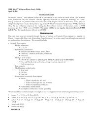
Throttling loss"<br />
Throttling loss increases from zero at wide-open throttle (WOT) to about<br />
half of all fuel usage at idle (other half is friction loss)<br />
At typical highway cruise condition (≈ 1/3 of BMEP at WOT), about 15%<br />
loss due to throttling (side topic: throttleless premixed-charge engines)<br />
Throttling isn’t always bad, when you take your foot off the gas pedal &<br />
shift to a lower gear to reduce vehicle speed, youre using throttling loss<br />
(negative BMEP) and high N to maximize negative power<br />
1<br />
0.9<br />
! 0.85<br />
Double-click plot!<br />
To open Excel chart!<br />
Efficiency (with throttle) /<br />
Efficiency (without throttle)<br />
0.8<br />
0.7<br />
0.6<br />
0.5<br />
0.4<br />
0.3<br />
0.2<br />
Typical highway cruise<br />
condition ! 1/3 of<br />
maximum BMEP<br />
K = IMEP/P intake = 9.1<br />
FMEP = 10 psi<br />
P ambient = 14.7 psi<br />
0.1<br />
0<br />
0 0.2 0.4 0.6 0.8 1<br />
BMEP / BMEP at wide open throttle<br />
<strong>AME</strong> <strong>436</strong> - Lecture 8 - Spring 2013 - Ideal cycle analysis<br />
16<br />
• 8
Throttling loss"<br />
Another way to reduce throttling losses: close off some<br />
cylinders when low power demand<br />
Cadillac had a 4-6-8 engine in the 1981 but it was a mechanical<br />
disaster<br />
Mercedes had Cylinder deactivation on V12 engines in 2001 -<br />
2002<br />
GM uses a 4-8 Active Fuel Management (previously called<br />
Displacement On Demand) engine<br />
Nowadays several manufacturers have variable displacement<br />
engines (e.g Chrysler 5.7 L Hemi, Multi-Displacement System)<br />
Good summary article on the mechanical aspects of variable<br />
displacement:<br />
http://www.autospeed.com/A_2618/xBXyt34qy_1/cms/article.html<br />
Certainly reduces throttling loss, but still have friction losses in<br />
inoperative cylinders<br />
<strong>AME</strong> <strong>436</strong> - Lecture 8 - Spring 2013 - Ideal cycle analysis<br />
17<br />
Throttling loss"<br />
Many auto magazines suggest cylinder deactivation will cut fuel<br />
usage in half, as if engines use fuel based only on displacement, not<br />
RPM (N) or intake manifold pressure - more realistic reports suggest<br />
8 - 10% improvement in efficiency<br />
Aircycles4recips.xls (to be introduced in next lecture) analysis<br />
Defaults: r = 9, V d = 0.5 liter, P intake = 1 atm, FMEP = 1 atm)<br />
Predictions: P intake = 1 atm, 13.45 hp, η = 29.96%<br />
1/3 of max. power via throttling: P intake = 0.445 atm, 4.48 hp, η = 22.42%<br />
1/3 of max. power via halving displacement<br />
(double FMEP to account for friction losses in inoperative cylinders)<br />
P intake = 0.806 atm, 4.48 hp, η = 24.78%<br />
(10.3% improvement over throttling)<br />
Smaller engine operating at wide-open throttle to get same power:<br />
V d = 0.5 liter / 3 = 0.167 liter, 4.48 hp, η = 29.96%<br />
(33.6% improvement over throttling bigger engine)<br />
Moral: if we all drove under-powered cars (small displacement)<br />
we’d get much better gas mileage than larger cars with variable<br />
displacement – could use turbocharging to regain maximum power<br />
Hybrids use the wide-open throttle, small displacement idea and<br />
store surplus power in battery<br />
<strong>AME</strong> <strong>436</strong> - Lecture 8 - Spring 2013 - Ideal cycle analysis 18<br />
• 9
Turbocharging & supercharging"<br />
Best way to increase power is to increase intake air pressure above<br />
ambient using an air pump that forces air into the engine at P in ><br />
ambient<br />
Instead of having a pumping loss, you have a pumping gain! <br />
Turbocharging: instead of blowdown (5 → 6), divert exhaust gas<br />
through a turbine & use shaft power to drive air pump; since use is<br />
made of high pressure gas that is otherwise wasted during<br />
blowdown, thermal efficiency can actually be increased<br />
Supercharging: air pump is driven directly from the engine rather<br />
than a separate turbine; if pump is 100% efficient (yeah, right…)<br />
then no loss of overall cycle efficiency<br />
Limitations / problems<br />
To get maximum benefit, need intercooler to cool intake air (thus<br />
increase density) after compression but before entering engine<br />
Need time to overcome inertia of rotating parts & fill intake manifold<br />
with high-pressure air (turbo lag)<br />
Turbochargers: moving parts in hot exhaust system - not durable<br />
Cost, complexity<br />
If an engine isnt turbocharged or supercharged, its called<br />
naturally aspirated<br />
<strong>AME</strong> <strong>436</strong> - Lecture 8 - Spring 2013 - Ideal cycle analysis<br />
19<br />
Turbocharging & supercharging"<br />
Source: http://auto.howstuffworks.com/turbo.htm<br />
<strong>AME</strong> <strong>436</strong> - Lecture 8 - Spring 2013 - Ideal cycle analysis<br />
20<br />
• 10
Turbocharging & supercharging"<br />
35.0<br />
30.0<br />
Compression Combustion Expansion<br />
Blowdown Intake Exhaust<br />
Intake start 1 2<br />
3 4 5<br />
6 7<br />
P-V diagram<br />
Pressure (atm)<br />
25.0<br />
20.0<br />
15.0<br />
10.0<br />
5.0<br />
Pumping gain<br />
Work available<br />
to turbocharger<br />
0.0<br />
0.E+00 1.E-04 2.E-04 3.E-04 4.E-04 5.E-04 6.E-04<br />
Cylinder volume (m^3)<br />
<strong>AME</strong> <strong>436</strong> - Lecture 8 - Spring 2013 - Ideal cycle analysis<br />
21<br />
Turbocharging & supercharging"<br />
Compression Combustion Expansion<br />
Blowdown Intake Exhaust<br />
Close T-s cycle 1 2<br />
3 4 5<br />
6<br />
1200<br />
7<br />
T-s diagram<br />
1000<br />
Temperature (K)<br />
800<br />
600<br />
400<br />
v<br />
200<br />
Blowdown becomes<br />
expansion process for turbine<br />
0<br />
-100 0 100 200 300 400 500 600 700<br />
Entropy (J/kg-K)<br />
<strong>AME</strong> <strong>436</strong> - Lecture 8 - Spring 2013 - Ideal cycle analysis<br />
P<br />
22<br />
• 11
Why use Diesel cycle to model nonpremixed-charge engines"<br />
Volume compression ratio = (volume ratio during heat addition) x<br />
(volume expansion ratio) as with reciprocating piston/cylinder<br />
arrangement (same reason as Otto/premixed)<br />
Heat input at constant pressure corresponds to slower combustion<br />
than constant-volume combustion - not exactly true for real engine,<br />
but represents slower combustion than premixed-charge engine<br />
while still maintaining simple cycle analysis<br />
Diesels have slower combustion since fuel is injected after<br />
compression, thus need to mix and burn, instead of just burn<br />
(already mixed before spark is fired) in premixed-charge engine<br />
As always, constant s compression/expansion corresponds to an<br />
adiabatic and reversible process - not exactly true but not bad<br />
either<br />
Diesels not throttled (for reasons discussed later) (though often<br />
turbo/supercharged)<br />
<strong>AME</strong> <strong>436</strong> - Lecture 8 - Spring 2013 - Ideal cycle analysis<br />
23<br />
Ideal Diesel cycle analysis"<br />
Compression ratio r = V 1 /V 2 = V 2 /V 3 = V 5 /V 3 = V 6 /V 7<br />
New parameter: Cutoff ratio β = V 4 /V 3 ; since 3 → 4 is const. P not const. V<br />
β = V 4 /V 3 = (mRT 4 /P 4 )/(mRT 3 /P 3 ) = T 4 /T 3 (Cutoff ratio β not to be confused with nondimensional<br />
activation energy β)<br />
Stroke Process Name Constant Mass in<br />
cylinder<br />
Other info<br />
A 1 → 2 Intake P Increases P 2 = P 1 ; T 2 = T 1<br />
At 1, exhaust valve opens,<br />
intake valve closes<br />
B 2 → 3 Compression s Constant P 3 /P 2 = r γ ; T 3 /T 2 = r (γ-1)<br />
At 2, intake valve closes<br />
--- 3→ 4 Combustion P Constant T 4 = T 3 + fQ R /C P ;<br />
T 4 /T 3 = V 4 /V 3<br />
At 3, fuel is injected<br />
C 4 → 5 Expansion s Constant P 4 /P 5 = (r/β) γ ; T 4 /T 5 = (r/β) (γ-1)<br />
--- 5 → 6 Blowdown V Decreases P 6 = P ambient ;<br />
T 6 /T 5 = (P 6 /P 5 ) (γ-1)/γ<br />
At 5, exhaust valve opens,<br />
exhaust gas blows down<br />
as with Otto<br />
D 6 → 7 Exhaust P Decreases P 7 = P 6 ; T 7 = T 6<br />
<strong>AME</strong> <strong>436</strong> - Lecture 8 - Spring 2013 - Ideal cycle analysis<br />
24<br />
• 12
P-V & T-s diagrams for ideal Diesel cycle"<br />
Work is done during both 4 → 5 AND 3 → 4 (const. P combustion,<br />
volume increasing, thus w 3→4 = P 3 (v 4 - v 3 )<br />
Ambient intake pressure case shown (no pumping loop)<br />
Pressure (atm)<br />
5.0<br />
4.5<br />
4.0<br />
3.5<br />
3.0<br />
2.5<br />
2.0<br />
1.5<br />
1.0<br />
0.5<br />
Compression Combustion Expansion<br />
Blowdown Intake Exhaust<br />
Intake start 1 2<br />
3 4 5<br />
6 7<br />
P-V diagram<br />
0.0<br />
0.E+00 1.E-04 2.E-04 3.E-04 4.E-04 5.E-04 6.E-04<br />
Cylinder volume (m^3)<br />
Temperature (K)<br />
Compression Combustion Expansion<br />
Blowdown Intake Exhaust<br />
Close T-s cycle 1 2<br />
3 4 5<br />
6 7<br />
1000<br />
900 T-s diagram<br />
800<br />
700<br />
600<br />
500<br />
400<br />
300<br />
200<br />
100<br />
0<br />
-200 0 200 400 600 800<br />
Entropy (J/kg-K)<br />
<strong>AME</strong> <strong>436</strong> - Lecture 8 - Spring 2013 - Ideal cycle analysis<br />
25<br />
Diesel cycle analysis"<br />
Thermal efficiency (ideal cycle, no throttling or friction loss)<br />
work out + work in<br />
" th<br />
= = C (T # T ) + P (v # v ) + C (T # T )<br />
v 4 5 4 4 3 v 2 3<br />
heat in<br />
C P<br />
(T 4<br />
# T 3<br />
)<br />
= (T 4 # T 5 ) + (R /C v )(T 4 # T 3 ) # (T 3 # T 2 )<br />
(C P<br />
/C v<br />
)(T 4<br />
# T 3<br />
)<br />
=1# 1 $ + T 4 (1# (V 5 /V 4 )#($ #1) ) # T 3<br />
(1# (V 2<br />
/V 3<br />
) #($ #1) )<br />
$(T 4<br />
# T 3<br />
)<br />
=1# 1 $ + 1 $ + T 4 (#(V 5 /V 4 )#($ #1) ) + T 3<br />
((V 2<br />
/V 3<br />
) #($ #1) )<br />
$(T 4<br />
# T 3<br />
)<br />
=1+ #T 4<br />
([(V 5<br />
/V 3<br />
)(V 3<br />
/V 4<br />
)] #($ #1) ) + T 3<br />
((V 2<br />
/V 3<br />
) #($ #1) )<br />
$(T 4<br />
# T 3<br />
)<br />
=1+ #T 4<br />
([r /%] #($ #1) ) + T 3<br />
(r #($ #1) )<br />
$(T 4<br />
# T 3<br />
)<br />
= $ #1 + T (1# T /T ) # T (1# T /T )<br />
4 5 4 3 2 3<br />
$<br />
$(T 4<br />
# T 3<br />
)<br />
=1+ #%T 3([r /%] #($ #1) ) + T 3<br />
(r #($ #1) )<br />
$(%T 3<br />
# T 3<br />
)<br />
=1# %([r /%]#($ #1) ) # (r #($ #1) )<br />
=1# 1 % $ #1<br />
$(% #1)<br />
r $ #1 $(% #1)<br />
<strong>AME</strong> <strong>436</strong> - Lecture 8 - Spring 2013 - Ideal cycle analysis<br />
26<br />
!<br />
• 13
!<br />
Otto vs. Diesel cycle comparison"<br />
Thermal efficiency (ideal cycle, no throttling or friction loss)<br />
" th,Diesel<br />
=1# 1 & % $ #1 )<br />
r $ #1 ( + ; recall "<br />
' $ (% #1)<br />
th,Otto<br />
=1# 1<br />
*<br />
r ( 1)<br />
$ #1<br />
% $ #1<br />
$(% #1) >1 for % >1,$ >1; % $ #1<br />
,1 as % ,1<br />
$ (% #1)<br />
⇒ For same r, η th (Otto) > η th (Diesel)<br />
⇒ η th (Otto) ≈ η th (Diesel) as β → 1 (small heat input)<br />
Lower η th is due to burning at increasing volume, thus decreasing T<br />
- thus less efficient Carnot-cycle strips; most efficient burning<br />
strategy is at minimum volume, thus maximum T<br />
Note that (unlike Otto cycle) η th is dependent on the heat input<br />
! V 4<br />
= T 4<br />
=1+ T 4<br />
"T 3<br />
=1+ fQ R<br />
/ C P<br />
fQ<br />
=1+ R<br />
V 3<br />
T 3<br />
T 2<br />
r ""1<br />
T 3<br />
Higher heat input ⇒ higher f ⇒ larger β ⇒ lower η th<br />
<strong>AME</strong> <strong>436</strong> - Lecture 8 - Spring 2013 - Ideal cycle analysis<br />
27<br />
!<br />
C P<br />
T 2<br />
r ""1<br />
Must have V 4 /V 3 ≤ V 5 /V 3 (otherwise burning is still occurring at<br />
bottom of piston travel) end of thus β ≤ r<br />
fQ<br />
" # r $ 1+ R<br />
C P<br />
T 2<br />
r # r $ f # (r &1)C PT 2<br />
r % &1<br />
% &1 Q R<br />
For r = 20, Q R = 4.3 x 10 7 J/kg, C P = 1400 J/kgK, γ = 1.3, T 2 = 300K,<br />
requirement is f < 0.417, which is much greater than stoichiometric f<br />
(≈ 0.065) anyway so in practice this limit is never reached<br />
Typical f ≈ 0.04 (with other parameters as above): β ≈ 2.67, η th ≈<br />
0.515 (Diesel) vs. 0.593 (Otto), so difference not large for realistic<br />
conditions<br />
As with Otto, η th increases as r increases - why not use r → ∞<br />
(η th → 1) Unlike Otto, knock is not an issue - Diesel compresses<br />
air, not fuel/air mixture; main reason: heat losses<br />
Since knock is not an issue, Diesels use much higher r<br />
As gas is compressed more, T increases and volume of gas<br />
decreases, increasing ΔT/ΔX for conduction loss<br />
As conduction loss increases, compression work lost increases<br />
At some point, lost work outweighs inherently higher η th of cycle<br />
having higher r<br />
Also - as r increases, peak pressure increases - larger mechanical<br />
stresses for little improvement in η th<br />
<strong>AME</strong> <strong>436</strong> - Lecture 8 - Spring 2013 - Ideal cycle analysis 28<br />
Otto vs. Diesel cycle comparison"<br />
• 14
Otto vs. Diesel cycle comparison"<br />
Pressure (atm)<br />
12.0<br />
10.0<br />
8.0<br />
6.0<br />
4.0<br />
2.0<br />
Compression Combustion Expansion<br />
Blowdown Intake Exhaust<br />
Intake start 1 2<br />
3 4 5<br />
6 7<br />
Otto<br />
Diesel<br />
P-V diagram<br />
0.0<br />
0.E+00 1.E-04 2.E-04 3.E-04 4.E-04 5.E-04 6.E-04<br />
Cylinder volume (m^3)<br />
Unthrottled Otto & Diesel with same compression ratio & heat<br />
input: Otto has higher peak P & T, more work output<br />
<strong>AME</strong> <strong>436</strong> - Lecture 8 - Spring 2013 - Ideal cycle analysis<br />
29<br />
Temperature (K)<br />
1200<br />
1000<br />
800<br />
600<br />
400<br />
200<br />
Compression Combustion Expansion<br />
Blowdown Intake Exhaust<br />
Close T-s cycle 1 2<br />
3 4 5<br />
6 7<br />
Otto vs. Diesel cycle (animation)"<br />
T-s diagram<br />
Equal areas<br />
Diesel<br />
Otto<br />
Otto work<br />
Diesel work<br />
Otto heat input<br />
Diesel heat input<br />
0<br />
-200 0 200 400 600 800<br />
Entropy (J/kg-K)<br />
Otto clearly has higher η th - every Carnot strip has same T L for both<br />
cycles, but every Otto strip has higher T H<br />
Unlike Otto cycle, η th for Diesel cannot be determined by inspection of the<br />
T - s diagram since each Carnot cycle strip has a different 1 - T L /T H<br />
<strong>AME</strong> <strong>436</strong> - Lecture 8 - Spring 2013 - Ideal cycle analysis<br />
30<br />
• 15
Effect of compression ratio (Diesel)"<br />
Animation: P-V diagrams, increasing compression ratio (same<br />
displacement volume, same fuel mass fraction (f), thus same heat input)<br />
Pressure (atm)<br />
14.0<br />
12.0<br />
10.0<br />
8.0<br />
6.0<br />
4.0<br />
Compression Combustion Expansion<br />
Blowdown Intake Exhaust<br />
Intake start 1 2<br />
3 4 5<br />
6 7<br />
P-V diagram<br />
P-V diagram<br />
(high (low compression)<br />
(medium compression)<br />
2.0<br />
0.0<br />
0.0E+00 2.0E-03 4.0E-03 6.0E-03 8.0E-03 1.0E-02 1.2E-02<br />
Cylinder volume (m^3)<br />
<strong>AME</strong> <strong>436</strong> - Lecture 8 - Spring 2013 - Ideal cycle analysis<br />
31<br />
Effect of compression ratio (Diesel)"<br />
Animation: T-s diagrams, increasing compression ratio (same<br />
displacement volume, same fuel mass fraction (f), thus same heat input)<br />
Higher compression clearly more efficient (taller Carnot strips)<br />
800<br />
Compression Combustion Expansion<br />
Blowdown Intake Exhaust<br />
Close T-s cycle 1 2<br />
3 4 5<br />
6 7<br />
700<br />
Temperature (K)<br />
600<br />
500<br />
400<br />
300<br />
200<br />
T-s diagram<br />
(medium (high (low compression)<br />
100<br />
0<br />
-100 0 100 200 300 400 500<br />
Entropy (J/kg-K)<br />
<strong>AME</strong> <strong>436</strong> - Lecture 8 - Spring 2013 - Ideal cycle analysis<br />
32<br />
• 16
Effect of heat input (Diesel)"<br />
Animation: P-V diagrams, increasing heat input via increasing f (same<br />
displacement volume, same compression ratio)<br />
Pressure (atm)<br />
8.0<br />
7.0<br />
6.0<br />
5.0<br />
4.0<br />
3.0<br />
2.0<br />
Compression Combustion Expansion<br />
Blowdown Intake Exhaust<br />
Intake start 1 2<br />
3 4 5<br />
6 7<br />
P-V diagram<br />
P-V diagram<br />
(high (low heat input)<br />
(medium heat<br />
1.0<br />
0.0<br />
0.0E+00 1.0E-03 2.0E-03 3.0E-03 4.0E-03 5.0E-03 6.0E-03<br />
Cylinder volume (m^3)<br />
<strong>AME</strong> <strong>436</strong> - Lecture 8 - Spring 2013 - Ideal cycle analysis<br />
33<br />
Effect of heat input (Diesel)"<br />
Animation: T-s diagrams, increasing heat input via increasing f (same<br />
displacement volume, same compression ratio)<br />
Heat input does affect efficiency (shrinking T L /T H in Carnot strips as f<br />
increases)<br />
800<br />
Compression Combustion Expansion<br />
Blowdown Intake Exhaust<br />
Close T-s cycle 1 2<br />
3 4 5<br />
6 7<br />
700<br />
Temperature (K)<br />
600<br />
500<br />
400<br />
300<br />
200<br />
T-s diagram<br />
(medium (high (low heat heat input)<br />
100<br />
0<br />
-100 0 100 200 300 400 500 600 700<br />
Entropy (J/kg-K)<br />
<strong>AME</strong> <strong>436</strong> - Lecture 8 - Spring 2013 - Ideal cycle analysis<br />
34<br />
• 17
Example"<br />
For an ideal Diesel cycle with the following parameters: r = 20, γ = 1.3, M = 0.029 kg/<br />
mole, f = 0.05, Q R = 4.45 x 10 7 J/kg, initial temperature T 2 = 300K, initial pressure P 2<br />
= 1 atm, P exh = 1 atm, determine:<br />
a) Temperature (T 3 ) & pressure (P 3 ) after compression & compression work per kg<br />
P 3<br />
P 2<br />
= r ! ! P 3<br />
= P 2<br />
r ! =1atm(20) 1.3 ! P 3<br />
= 49.1atm<br />
T 3<br />
= r !"1 ! T<br />
T<br />
3<br />
= T 2<br />
r !"1 = 300K ( 20) 1.3"1 ! T 3<br />
= 737K<br />
2<br />
W comp<br />
= "C v<br />
(T 3<br />
"T 2<br />
) = " R<br />
! "1 (T "T ) = " # 1<br />
8.314J / moleK 1<br />
(737 " 300) = " (737K " 300K)<br />
3 2<br />
M ! "1 0.029kg / mole 1.3"1<br />
W comp<br />
= "(955.6J / kgK)(737K " 300K) = "417.6kJ / kg (negative since work is into system)<br />
b) Temperature (T 4 ) and pressure (P 4 ) after combustion, and the work output<br />
during combustion per kg of mixture<br />
T 4<br />
= T 3<br />
+ fQ R<br />
;C<br />
C<br />
p<br />
= !<br />
p<br />
! !1 R = 1.3 8.314J / moleK<br />
1.3!1 0.029kg / mole = 1242J<br />
kgK<br />
$ v '<br />
P 4<br />
= P 3<br />
= 49.1atm " W comb<br />
= P(v 4<br />
! v 3<br />
) = Pv 4<br />
3 & !1<br />
% v<br />
)<br />
3 (<br />
= RT $ T '<br />
4<br />
!1<br />
3&<br />
% T<br />
)<br />
3 (<br />
= R T !T 4 3<br />
W comb<br />
=<br />
8.314J / moleK<br />
0.029kg / mole<br />
( 2528K ! 737K) = +513.5kJ / kg<br />
" T = 737K + (0.05)(4.45#107 J / kg)<br />
= 2528K<br />
4<br />
1242J / kgK<br />
( ) = * (<br />
M T !T 4 3)<br />
<strong>AME</strong> <strong>436</strong> - Lecture 8 - Spring 2013 - Ideal cycle analysis<br />
35<br />
!<br />
!<br />
Example (continued)"<br />
c) Cutoff Ratio<br />
" = V 4<br />
= V 4<br />
m<br />
= RT )1<br />
#<br />
3<br />
P 4<br />
&<br />
% ( = T 4<br />
= 2528K<br />
V 3<br />
m V 3 $ P 3<br />
RT 4 ' T 3<br />
737K = 3.43<br />
d) Temperature (T 5 ) and pressure (P 5 ) after expansion, and the expansion work per kg of<br />
mixture<br />
P 4<br />
= r )<br />
# & #<br />
% ( = 20 &<br />
1.3<br />
% ( = 9.89 * P<br />
P 5 $ " ' $ 3.43'<br />
5<br />
= P 4<br />
9.89 = 49.1atm = 4.96atm<br />
9.89<br />
T 4<br />
#<br />
= r &<br />
% (<br />
T 5 $ " '<br />
) +1<br />
W exp<br />
= +C V<br />
T 5<br />
+ T 4<br />
= ( 5.83) 1.3+1 =1.7 * T 5<br />
= T 4<br />
1.7 = 2528K =1489K<br />
1.7<br />
( ) = +955.63J /kgK( 1489K + 2528K) = 992.9kJ /kg<br />
e) Net work per kg of mixture<br />
Net work = Compression work + Work during combustion + Expansion work<br />
= -417.6 + 992.9 + 513.5 = 1089 kJ/kg<br />
<strong>AME</strong> <strong>436</strong> - Lecture 8 - Spring 2013 - Ideal cycle analysis<br />
36<br />
• 18
Example (continued)"<br />
f) Thermal Efficiency<br />
η th = (Net work per unit mass) / (Heat input per unit mass)<br />
= (Net work)/fQ R = (1.089 x 10 6 J/kg)/(0.05)(4.45 x 10 7 J/kg) = 0.489 = 48.9%<br />
compare this to the theoretical efficiency (should be the same since this is an ideal<br />
cycle analysis)<br />
" th<br />
=1# 1 & % $ #1 ) 1 & 3.43 1.3 #1 )<br />
( + =1# ( + = 0.489 = 48.9%<br />
r $ #1 ' $ (% #1)<br />
* 20 1.3#1 ' 1.3( 3.43 #1)<br />
*<br />
g) IMEP<br />
!<br />
!<br />
Net work<br />
IMEP = =<br />
V d<br />
(Net work)/mass<br />
=<br />
V d<br />
/mass<br />
Net work/mass<br />
= "<br />
V d<br />
/(" 2<br />
V d<br />
)<br />
2<br />
(Net work/mass)<br />
P<br />
# IMEP = 2<br />
1.089 %10 6 J /kg<br />
(Net work/mass) =<br />
=12.7atm<br />
($/ M)T 2<br />
[(8.314J /moleK) /(0.029kg /mole)](300K)<br />
1atm<br />
Note that the mass does not include the mass in the clearance volume; it is<br />
assumed that this mass is inert (i.e. exhaust gas) which does not yield additional heat<br />
release, plus its compression/expansion work cancel out<br />
<strong>AME</strong> <strong>436</strong> - Lecture 8 - Spring 2013 - Ideal cycle analysis<br />
37<br />
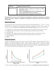
Examples of using P-V & T-s diagrams"<br />
Consider the “baseline ideal Diesel cycle shown on the P-V and T-s diagrams. Sketch<br />
modified diagrams if the following changes are made. Unless otherwise noted, assume in<br />
each case the initial T & P, r, f, Q R , etc. are unchanged.<br />
a) The compression ratio is increased (same maximum volume)<br />
Equal<br />
areas<br />
The minimum volume must decrease since r increases but the maximum volume does not.<br />
The cutoff ratio = 1 + fQ R /C P T 2 r γ-1 decreases. The temperature after compression T 3 as<br />
well as the maximum temperature T 4 = T 3 + fQ R /C P increase. In order to maintain equal<br />
heat addition and thus equal areas on the T-s diagram, s 4 decreases.<br />
<strong>AME</strong> <strong>436</strong> - Lecture 8 - Spring 2013 - Ideal cycle analysis<br />
38<br />
• 19
Examples of using P-V & T-s diagrams"<br />
b) Part way through the constant-pressure burn, the remainder of the burn occurs<br />
instantaneously at constant volume<br />
Higher max. T for<br />
modified cycle<br />
v<br />
Equal<br />
areas<br />
The cycle is the same until the 2 nd part of the burn occurs at constant volume<br />
rather than constant pressure, which has a higher slope. To maintain the same<br />
total heat release, s 4 must decrease. Also, because constant volume combustion<br />
results in higher T than constant pressure combustion, the maximum T increases<br />
<strong>AME</strong> <strong>436</strong> - Lecture 8 - Spring 2013 - Ideal cycle analysis<br />
39<br />
Examples of using P-V & T-s diagrams"<br />
c) The intake valve closes late (i.e. after part of the compression stroke has started;<br />
the pressure stays at ambient pressure and no compression occurs until after the<br />
intake valve closes) in such a way that the pressure after the expansion is ambient.<br />
Lower max. T for<br />
modified cycle<br />
v<br />
P<br />
Equal<br />
areas<br />
In order to have the pressure after expansion be ambient, the P-V curve for the<br />
expansion part of the modified cycle must be the same as the compression part of<br />
the base cycle. The pressure remains at ambient part way through the compression<br />
stroke, until the intake valve closes. The compression ratio is lower, thus the P and<br />
T after compression (state 3) are lower. s 4 must increase in order for the heat<br />
release (thus area) of the modified cycle to be the same as that of the baseline cycle.<br />
<strong>AME</strong> <strong>436</strong> - Lecture 8 - Spring 2013 - Ideal cycle analysis<br />
40<br />
• 20
Complete expansion cycle"<br />
Highest efficiency cycle consistent with piston/cylinder engine has<br />
constant-V combustion but expansion back to ambient P - complete<br />
expansion or Atkinson cycle (caution: different sources have<br />
different cycle naming conventions – Atkinson, Humphrey, Miller etc.<br />
– wikipedia.com is becoming the new default standard!)<br />
Needs different compression & expansion ratios - can be done by<br />
closing the intake valve AFTER the compression starts or by<br />
extracting power in a turbine whose work is somehow connected to<br />
the main shaft power output<br />
Pressure (atm)<br />
Pressure (atm)<br />
Compression Combustion Expansion<br />
Blowdown Compression Intake Combustion Exhaust Expansion<br />
Intake Blowdown start 1 Intake 2 Exhaust<br />
3 Intake start 4 1 5 2<br />
6 3 7 4 5<br />
12.0<br />
12.0<br />
6 7<br />
P-V diagram<br />
P-V diagram<br />
10.0<br />
10.0<br />
8.0<br />
8.0<br />
6.0<br />
6.0<br />
4.0<br />
4.0<br />
2.0<br />
2.0<br />
0.0<br />
0.0<br />
0.E+00 2.E-04 4.E-04 6.E-04 8.E-04 1.E-03<br />
0.E+00 2.E-04 4.E-04 6.E-04 8.E-04<br />
Cylinder volume (m^3)<br />
1.E-03<br />
Cylinder volume (m^3)<br />
1200<br />
r compression = 3<br />
r expansion = 5.5<br />
Dont forget this -work<br />
when computing η!<br />
T-s diagram<br />
Compression Combustion Expansion<br />
Blowdown<br />
Close T-s cycle<br />
Temperature (K)<br />
Compression Combustion Expansion<br />
Blowdown Intake Exhaust<br />
Close T-s cycle 1 2<br />
3 4 5<br />
6 7<br />
1200<br />
T-s diagram<br />
1000<br />
800<br />
600<br />
400<br />
200<br />
0<br />
constant v<br />
constant P<br />
-200 0 200 400 600 800<br />
Entropy (J/kg-K)<br />
<strong>AME</strong> <strong>436</strong> - Lecture 8 - Spring 2013 - Ideal cycle analysis<br />
41<br />
1000<br />
Complete expansion cycle analysis"<br />
Temperature (K)<br />
800<br />
Isentropic compression: V 3<br />
= V 2<br />
/ r c<br />
; T 3<br />
= T 2<br />
r c !!1 ;P 3<br />
= P 2<br />
r c<br />
!<br />
600<br />
Constant volume combustion: V 4<br />
= V 3<br />
400<br />
T 4<br />
= T 3<br />
+ fQ R<br />
= T 2<br />
r !!1 c<br />
+ fQ "<br />
R<br />
= T 2<br />
r !!1 fQ<br />
c<br />
1+ R<br />
%<br />
$<br />
!!1<br />
' = 1+! " !1<br />
C V # C V<br />
T 2<br />
r c &<br />
200 C V<br />
Recall from Diesel cycle analysis: " =1+<br />
fQ R<br />
0<br />
-100 0 100 200 300 400 500 600 700<br />
Entropy (J/kg-K)<br />
C P<br />
T 2<br />
r !!1<br />
" T<br />
P 4<br />
= P 4<br />
%<br />
3 $<br />
# T 3 &<br />
' = P r " T r !!1 (1+! ( " !1 ))%<br />
! 2 c<br />
2 c $<br />
!!1<br />
# T 2<br />
r<br />
'<br />
c &<br />
= P !<br />
2r c<br />
( ( ))<br />
( 1+! (" !1))<br />
Isentropic expansion: P 5<br />
= P 2<br />
, expansion ratio r e<br />
= V 4<br />
/V 5<br />
> r c<br />
( ( ))<br />
1 !<br />
= r c ( 1+! (" !1)) 1 !<br />
or r e<br />
P 4<br />
= P 5<br />
r ! e<br />
( r e<br />
= P 1<br />
" % ! "<br />
4<br />
$ ' = P !<br />
2r c<br />
1+! " !1 %<br />
# P 5 &<br />
$<br />
# P '<br />
2 &<br />
T 4<br />
= T 5<br />
r !!1 e<br />
( T 5<br />
= T 4<br />
r = T 2r !!1 c<br />
(1+! (" !1))<br />
!!1<br />
e )<br />
r c ( 1+! (" !1)) 1 ! ,<br />
= T !!1 2<br />
1+! " !1<br />
*+<br />
-.<br />
( ( )) 1 !<br />
( ( )) 1 !<br />
r c<br />
= 1+! " !1<br />
<strong>AME</strong> <strong>436</strong> - Lecture 8 - Spring 2013 - Ideal cycle analysis<br />
42<br />
• 21
Complete expansion cycle analysis"<br />
net work<br />
! th<br />
=<br />
heat in = C v(T 4<br />
!T 5<br />
)+ C v<br />
(T 2<br />
!T 3<br />
)+ P 2<br />
(v 2<br />
! v 5<br />
)<br />
C v<br />
(T 4<br />
!T 3<br />
)<br />
"<br />
Note P 2<br />
(v 2<br />
! v 5<br />
) = P 2<br />
v 2<br />
1! v 5<br />
v 4<br />
% ( "<br />
$ ' = RT 2<br />
1! P 2<br />
v 2<br />
1! v 5<br />
v 4<br />
% + "<br />
* $ '- = RT 2<br />
1! r %<br />
e<br />
(<br />
$ ' = RT 2<br />
1! (1+! (" !1)) 1 ! +<br />
# v 4<br />
v 2 & ) # v 4<br />
v 2 &,<br />
# r c & )*<br />
,-<br />
T 4<br />
!T 5<br />
+T 2<br />
!T 3<br />
+ RT 2<br />
(<br />
1! (1+! (" !1)) 1 ! +<br />
C<br />
" th<br />
=<br />
v<br />
)*<br />
,-<br />
T 4<br />
!T 3<br />
T 2<br />
r !!1 c<br />
(1+! (" !1))!T 2<br />
(1+! (" !1)) 1! (<br />
+T 2<br />
!T 2<br />
r !!1 c<br />
+ (! !1)T 2<br />
1! (1+! (" !1)) 1 ! +<br />
)*<br />
,-<br />
=<br />
fQ R<br />
/ C v<br />
=<br />
( 1+! (" !1)) !<br />
! (" !1) ! 1<br />
=<br />
! th<br />
=1! 1<br />
r c<br />
!!1<br />
( ( ))<br />
1 !<br />
1+! " !1<br />
+ 1 ! !1(<br />
!1+ 1! 1+! " !1<br />
!!1 !!1 !!1<br />
r c<br />
r c<br />
r c<br />
)*<br />
(<br />
1+! " !1<br />
!!1<br />
r c<br />
)*<br />
fQ R<br />
/ C v<br />
T 2<br />
r c<br />
!!1<br />
( ( )) 1 !<br />
( ( )) 1 ! + (<br />
!1 + (! !1) 1+! " !1<br />
,- ( ( ))<br />
1 ! +<br />
{ !1<br />
)*<br />
,- }<br />
! (" !1)<br />
( 1+! (" !1)) 1 !<br />
!1<br />
(" !1)<br />
(finally!)<br />
<strong>AME</strong> <strong>436</strong> - Lecture 8 - Spring 2013 - Ideal cycle analysis<br />
+<br />
,-<br />
43<br />
Otto vs. Complete exp. cycle comparison"<br />
Thermal efficiency (ideal cycle, no throttling or friction loss)<br />
! th,Atkinson<br />
= ! th<br />
=1! 1 "<br />
( 1+" (# !1)) 1 " %<br />
$<br />
!1'<br />
"!1<br />
r $<br />
c<br />
# !1 ' ; recall ! =1! 1<br />
th,Otto "!1 ( 1)<br />
r<br />
#<br />
&<br />
c<br />
( 1+" (# !1)) 1 "<br />
!1<br />
>1 for # >1 (1! 1 "<br />
( 1+" (# !1)) 1 " %<br />
$<br />
!1'<br />
"!1<br />
# !1<br />
r $<br />
c<br />
# !1 ' >1! 1<br />
"!1 ( 1)<br />
r<br />
#<br />
& c<br />
( 1+" (# !1)) 1 "<br />
!1<br />
)1 as # )1 ( ! th,Atkinson<br />
=1! 1<br />
"!1 ( 1)<br />
# !1<br />
r c<br />
( ) 1 "<br />
!1<br />
1+" (# !1)<br />
" 1 "<br />
) " ) 0 as # ) * ( !<br />
# !1<br />
(# !1) "!1 th,Atkinson<br />
)1<br />
"<br />
⇒ For same r c , η th (Complete expansion) > η th (Otto)<br />
⇒ η th (Complete expansion) ≈ η th (Otto) as β → 0 (small heat input)<br />
Like Diesel, Complete Expansion and Otto converge to same cycle at small<br />
heat input due to complete expansion (same T H & T L as Otto)<br />
Note that (unlike Otto cycle, but like Diesel cycle) η th in Complete<br />
expansion cycle is dependent on the heat input (through β), but<br />
unlike Diesel cycle, η th,CompleteExp increases with increasing heat input<br />
<strong>AME</strong> <strong>436</strong> - Lecture 8 - Spring 2013 - Ideal cycle analysis<br />
44<br />
• 22
Complete expansion cycle"<br />
Thermodynamically, ideal complete expansion cycle is same as<br />
turbocharged cycle if you take turbine work as net work output<br />
rather than driving an air pump<br />
Gain due to complete expansion is substantial<br />
Low-r cycle ideal shown on page 41: η th = 0.424 vs. 0.356<br />
Realistic cycle parameters (next lecture): η th = 0.366 vs. 0.295<br />
No muffler needed if exhaust always leaves cylinder at 1 atm!<br />
Late intake valve closing is preferable (higher η th ) to throttling for<br />
part-load operation, but<br />
Mechanically much more complex<br />
Every power level requires a different intake valve closing time, thus a<br />
different r compression , thus a different r expansion<br />
Since intake valve is closed late, maximum mass flow is less than<br />
conventional Otto cycle, so less power - at higher power levels can’t<br />
sustain complete expansion cycle<br />
This is an alternative to throttling for premixed-charge engines, but<br />
why dont we even talk about throttling for Diesels (Answer in 2<br />
slides…)<br />
<strong>AME</strong> <strong>436</strong> - Lecture 8 - Spring 2013 - Ideal cycle analysis<br />
45<br />
Complete expansion cycle"<br />
What is kept constant in comparison below Clearance volume<br />
Complete expansion cycle provides higher BMEP (based on V d for<br />
maximum-power cycle) AND higher efficiency, but at the expense of<br />
greatly increased mechanical complexity (and need for 2x larger<br />
piston stroke for wide-open throttle operation)<br />
Displacement-on-demand (1/2 displacement) similar to Complete<br />
Expansion, but doesn’t benefit high end of power range<br />
0.40<br />
1.0<br />
18<br />
Brake efficiency<br />
0.35<br />
0.30<br />
0.25<br />
0.20<br />
0.15<br />
0.10<br />
0.05<br />
0.00<br />
Throttled<br />
0 2 4 6 8 10 12 14<br />
BMEP (atm)<br />
Complete expansion<br />
Displacement on demand<br />
Intake Press (throttled or DoD)<br />
r c = 8 (throttled & DoD), γ = 1.3, f = 0.068, Q R = 4.5 x 10 7 J/kg, T in = 300K, P in = 1 atm (CE),<br />
P exh = 1 atm, ExhRes = TRUE, Const-v comb, BurnStart = 0.045, BurnEnd = 0.105, h =<br />
0.01, η comp = η exp = 0.9, FMEP = 1 atm<br />
<strong>AME</strong> <strong>436</strong> - Lecture 8 - Spring 2013 - Ideal cycle analysis 46<br />
0.9<br />
0.8<br />
0.7<br />
0.6<br />
0.5<br />
0.4<br />
0.3<br />
0.2<br />
0.1<br />
0.0<br />
0 2 4 6 8 10 12 14<br />
BMEP (atm)<br />
Throttled<br />
Displacement on demand<br />
rc (comp. exp. cycle)<br />
re (comp. exp. cycle)<br />
16<br />
14<br />
12<br />
10<br />
8<br />
6<br />
4<br />
2<br />
0<br />
rc or re (complete expansion)<br />
• 23
Ronney’s catechism (1/4)"<br />
Why do we throttle in a premixed charge engine despite the<br />
throttling losses it causes<br />
Because we have to reduce power & torque when we don’t want the full output of<br />
the engine (which is most of the time in LA traffic, or even on the open road)<br />
Why don’t we have to throttle in a nonpremixed charge engine<br />
Because we use control of the fuel to air ratio (i.e. to reduce power & torque, we<br />
reduce the fuel for the (fixed) air mass)<br />
Why don’t we do that for the premixed charge engine and avoid<br />
throttling losses<br />
Because if we try to burn lean in the premixed-charge engine, when the<br />
equivalence ratio (φ) is reduced below about 0.7, the mixture misfires and may<br />
stop altogether<br />
Why isn’t that a problem for the nonpremixed charge engine<br />
Nonpremixed-charge engines are not subject to flammability limits like premixedcharge<br />
engines since there is a continuously range of fuel-to-air ratios varying from<br />
zero in the pure air to infinite in the pure fuel, thus someplace there is a<br />
stoichiometric (φ = 1) mixture that can burn. Such variation in f does not occur in<br />
premixed-charge engines since, by definition, φ is the same everywhere.<br />
<strong>AME</strong> <strong>436</strong> - Lecture 8 - Spring 2013 - Ideal cycle analysis<br />
47<br />
Ronney’s catechism (2/4)"<br />
So why would anyone want to use a premixed-charge engine<br />
Because the nonpremixed-charge engine burns its fuel slower, since fuel and air<br />
must mix before they can burn. This is already taken care of in the premixedcharge<br />
engine. This means lower engine RPM and thus less power from an<br />
engine of a given displacement<br />
Wait - you said that the premixed-charge engine is slower burning.<br />
Only if the mixture is too lean. If it’s near-stoichiometric, then it’s faster because,<br />
again, mixing was already done before ignition (ideally, at least). Recall that as φ<br />
drops, T ad drops proportionately, and burning velocity (S L ) drops exponentially as<br />
T ad drops<br />
Couldn’t I operate my non-premixed charge engine at overall<br />
stoichiometric conditions to increase burning rate<br />
No. In nonpremixed-charge engines it still takes time to mix the pure fuel and<br />
pure air, so (as discussed previously) burning rates, flame lengths, etc. of<br />
nonpremixed flames are usually limited by mixing rates, not reaction rates. Worse<br />
still, with initially unmixed reactants at overall stoichiometric conditions, the last<br />
molecule of fuel will never find the last molecule of air in the time available for<br />
burning in the engine - one will be in the upper left corner of the cylinder, the<br />
other in the lower right corner. That means unburned or partially burned fuel<br />
would be emitted. That’s why diesel engines smoke at heavy load, when the<br />
mixture gets too close to overall stoichiometric.<br />
<strong>AME</strong> <strong>436</strong> - Lecture 8 - Spring 2013 - Ideal cycle analysis 48<br />
• 24
Ronney’s catechism (3/4)"<br />
So what wrong with operating at a maximum fuel to air ratio a<br />
little lean of stoichiometric<br />
That reduces maximum power, since you’re not burning every molecule of O 2<br />
in the cylinder. Remember - O 2 molecules take up a lot more space in the<br />
cylinder that fuel molecules do (since each O 2 is attached to 3.77 N 2<br />
molecules), so it behooves you to burn every last O 2 molecule if you want<br />
maximum power. So because of the mixing time as well as the need to run<br />
overall lean, Diesels have less power for a given displacement / weight / size /<br />
etc.<br />
So is the only advantage of the Diesel the better efficiency at<br />
part-load due to absence of throttling loss<br />
No, you also can go to higher compression ratios, which increases efficiency at<br />
any load. This helps alleviate the problem that slower burning in Diesels<br />
means lower inherent efficiency (more burning at increasing cylinder volume)<br />
Why can the compression ratio be higher in the Diesel engine<br />
Because you don’t have nearly as severe problems with knock. That’s because<br />
you compress only air, then inject fuel when you want it to burn. In the<br />
premixed-charge case, the mixture being compressed can explode (since it’s<br />
fuel + air) if you compress it too much<br />
<strong>AME</strong> <strong>436</strong> - Lecture 8 - Spring 2013 - Ideal cycle analysis<br />
49<br />
Ronney’s catechism (4/4)"<br />
Why is knock so bad<br />
We’ll discuss that in the section on knock<br />
So, why have things evolved such that small engines are usually<br />
premixed-charge, whereas large engines are nonpremixed-charge<br />
In small engines (lawn mowers, autos, etc.) you’re usually most concerned with getting the<br />
highest power/weight and power/volume ratios, rather than best efficiency (fuel economy).<br />
In larger engines (trucks, locomotives, tugboats, etc.) you don’t care as much about size and<br />
weight but efficiency is more critical<br />
But unsteady-flow aircraft engines, even large ones, are almost<br />
always premixed-charge, because weight is always critical in<br />
aircraft<br />
You got me on that one! (Though there is at least one production Diesel powered aircraft.)<br />
But of course most large aircraft engines are steady-flow gas turbines, which kill unsteadyflow<br />
engines in terms of power/weight and power/volume (but not efficiency.)<br />
<strong>AME</strong> <strong>436</strong> - Lecture 8 - Spring 2013 - Ideal cycle analysis<br />
50<br />
• 25
Fuel-air cycles"<br />
Up till now, we’ve only considered air cycles, where the<br />
properties of the gas (in particular C P , C v , γ) are assumed constant<br />
throughout the cycle (so that one can use relations like Pv γ =<br />
constant & T ad = T ∞ + fQ R /C v ) and heat is magically added to the gas<br />
at the appropriate point in the cycle<br />
This yields nice simple closed-form results, but isn’t very realistic<br />
We can get a more realistic estimate of performance by using real<br />
gas properties obtained from GASEQ or other chemical equilibrium<br />
programs<br />
Uses variable gas properties and compositions<br />
Shows that rich mixtures have low η th due to throwing away fuel that<br />
can’t be burned due to lack of O 2<br />
Shows limitation on work output because of limitation on what heat<br />
input combustion can provide<br />
Still doesn’t consider effects of<br />
Finite burning time (especially lean & rich mixtures)<br />
Incomplete combustion (crevice volumes, flame quenching, etc.)<br />
Heat & friction losses<br />
Hydrodynamic (pressure) losses in intake/exhaust<br />
Etc., etc.<br />
<strong>AME</strong> <strong>436</strong> - Lecture 8 - Spring 2013 - Ideal cycle analysis 51<br />
Fuel-air cycle analysis using GASEQ"<br />
Under Units menu, check mass, Joules and atm<br />
At the top of the page, under "Problem type" select "adiabatic compression/<br />
expansion" and make sure the box frozen composition is checked<br />
Under Reactants select appropriate set of reactants, e.g. Iso-octane-air flame<br />
To set the stoichiometry, first click on one of the species (e.g. the fuel), then to the<br />
right of the Stoichiometry box, click the button called set; in the dialog box that<br />
pops up, enter the equivalence ratio you want, then close the box<br />
Note (i.e. write down) the mass fraction of fuel<br />
In the box below the reactants box, enter the reactant temperature and pressure (e.g.<br />
298K, 1 atm) and the volume ratio of the compression process (e.g. 1/8 = 0.125 for<br />
compression ratio of 8) OR the final pressure (NOT pressure ratio) (e.g. 5 atm for a<br />
pressure ratio of 10 with reactants at 0.5 atm) in the locations provided<br />
Click on the "calculate" box. Note the internal energy, enthalpy and specific volume<br />
of both the reactants (call them u 2 , h 2 , v 2 ) and the products (u 3 , h 3 , v 3 )<br />
Click on the "R
Fuel-air cycle analysis using GASEQ"<br />
Click on the "R
Fuel-air cycle analysis"<br />
Efficiency<br />
0.7<br />
0.6<br />
0.5<br />
0.4<br />
0.3<br />
0.2<br />
0.1<br />
0.0<br />
Air-cycle<br />
Fuel-air cycle<br />
Gasoline engine, r = 8, T2 = 50C<br />
Iso-octane-air<br />
Otto cycle, r = 10<br />
T2 = 300K, P2 = 1 atm<br />
0 0.5 1 1.5 2 2.5 3 3.5<br />
Equivalence ratio<br />
Work/mass (kJ/kg) or<br />
maximum cycle T (K)<br />
3000<br />
2500<br />
2000<br />
1500<br />
1000<br />
500<br />
0<br />
work/mass (<br />
T4 (max. cyc<br />
work/mass (<br />
0 0.5 1 1.5 2 2<br />
Equivalence ratio<br />
<strong>AME</strong> <strong>436</strong> - Lecture 8 - Spring 2013 - Ideal cycle analysis<br />
55<br />
Efficiency<br />
0.7<br />
0.6<br />
0.5<br />
0.4<br />
0.3<br />
0.2<br />
0.1<br />
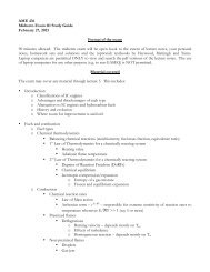
Fuel-air cycle analysis"<br />
BMEP = Work/V d = (Work/mass)/(V d /mass) = ρ intake (Work/mass)<br />
Work/mass or BMEP peaks at φ slightly > 1 (unlike η th which peaks at<br />
slightly < 1) - why Because BMEP is limited by the ability to burn all the<br />
O 2 , which is what takes up most of the space in the cylinder (each O 2<br />
attached to 3.77 N 2 , fuel occupies only ≈ 2% by moles or volume), so<br />
burning rich ensures all O 2 is burned<br />
Peak T is maximum at φ slightly > 1 for the same reason; outside the range<br />
0.6 < φ < 2, peak T is too low, ⇒ S L too low<br />
Air-cycle<br />
Fuel-air cycle<br />
Gasoline engine, r = 8, T2 = 50C<br />
Work/mass (kJ/kg) or<br />
maximum cycle T (K)<br />
3000<br />
2500<br />
2000<br />
1500<br />
1000<br />
500<br />
Iso-octane-air<br />
Otto cycle, r = 10<br />
T2 = 300K, P2 = 1 atm<br />
work/mass (Fuel-air cycle)<br />
T4 (max. cycle temp.)<br />
work/mass (real engine)<br />
0.0<br />
0 0.5 1 1.5 2 2.5 3 3.5<br />
Equivalence ratio<br />
0<br />
0 0.5 1 1.5 2 2.5 3 3.5<br />
Equivalence ratio<br />
<strong>AME</strong> <strong>436</strong> - Lecture 8 - Spring 2013 - Ideal cycle analysis<br />
56<br />
• 28
Example"<br />
Repeat the previous example of the ideal Diesel air-cycle analyis using a fuel-air cycle<br />
analysis (using GASEQ) with a stoichiometric iso-octane air mixture.<br />
P 2 = 1 atm, T 2 = 300K, f = 0.05 (φ = 0.792), u 2 =-172.54 kJ/kg, ρ 2 =1.2176 kg/m 3<br />
From GASEQ with Adiabatic Compression/Expansion, Frozen Chemistry, by<br />
trial and error find the pressure for which Volume Products/Volume Reactants =<br />
0.05 (r = 20). We obtain<br />
P 3 =53.7 atm, T 3 =805K, u 3 =260.17 kJ/kg, ρ 3 =24.366 kg/m 3<br />
Click R
Summary"<br />
Air-cycle analysis is very useful for understanding ICE performance<br />
P-v & T-s diagrams and numerical analysis are complementary<br />
Various cycles are used to model different real engines, but most<br />
involve isentropic compression/expansion and constant v or P heat<br />
addition<br />
Engines are air processors; more air processed ⇒ more power<br />
produced<br />
The differences between premixed (gasoline-type) and nonpremixed<br />
charge (diesel-type) combustion lead to major differences<br />
in performance and thus which applications for which each are<br />
most appropriate<br />
Power is controlled by air flow (via throttle) in premixed charge engines<br />
but via fuel/air ratio (FAR) in nonpremixed charge engines<br />
Compression ratio is limited by knock in premixed charge engines but<br />
by heat losses in nonpremixed charge engines<br />
Fuel-air cycles, where real gas properties are employed, are more<br />
realistic approximations than air cycles but still far removed from<br />
reality<br />
The ideal cycle analyses do NOT show the limitations of<br />
performance imposed by heat losses, slow burning, knock, friction,<br />
etc. - coming up in next 2 lectures<br />
<strong>AME</strong> <strong>436</strong> - Lecture 8 - Spring 2013 - Ideal cycle analysis<br />
59<br />
• 30