SOLUTION FOR HOMEWORK 10, STAT 4351 Welcome to your 10th ...

SOLUTION FOR HOMEWORK 10, STAT 4351
Welcome to your 10th (almost anniversary) homework. We begin our work on classical
continuous distributions.
As usual, try to find mistakes and get extra points!
Now let us look at your problems.
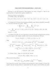
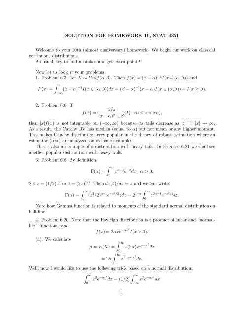
1. Problem 6.3. Let X ∼ Unif(α, β). Then f(x) = (β − α) −1 I(x ∈ (α, β)) and
F(x) =
∫ x
−∞
2. Problem 6.6. If
(β − α) −1 I(x ∈ (α, β))dx = (β − α) −1 (x − α)I(x ∈ (α, β)) + I(x ≥ β).
f(x) =
β/π
(x − α) 2 + β2I(−∞ < x < ∞),
then |x|f(x) is not integrable on (−∞, ∞) because its tails decrease as |x| −1 , |x| → ∞.
As a result, the Cauchy RV has median (equal to α) but not mean or any higher moment.
This makes Cauchy distribution very popular in the theory of robust estimation where an
estimator (test) are analyzed on extreme examples.
This is also an example of a distribution with heavy tails. In Exercise 6.21 we shall see
another popular distribution with heavy tails.
3. Problem 6.8. By definition,
Γ(α) =
∫ ∞
0
x α−1 e −x dx, α > 0.
Set x = (1/2)z 2 or z = (2x) 1/2 . Then dx(z)/dz = z and we can write:
Γ(α) =
∫ ∞
0
∫ ∞
(z 2 /2) α−1 e −z2 /2 zdz = 2 1−α z 2α−1 e −z2 /2 dz.
Note how Gamma function is related to moments of the standard normal distribution on
half-line.
4. Problem 6.20. Note that the Rayleigh distribution is a product of linear and “normallike”
functions, and
f(x) = 2αxe −αx2 I(x > 0).
(a). We calculate
µ = E(X) =
= 2α
∫ ∞
0
∫ ∞
0
0
x(2α)xe −αx2 dx
x 2 e −αx2 dx.
Well, now I would like to use the following trick based on a normal distribution:
∫ ∞
0
x 2 e −αx2 dx = (1/2)
1
∫ ∞
−∞
x 2 e −αx2 dx

= (1/2) (2π(2α)−1 ) 1/2
(2π(2α) −1 ) 1/2 ∫ ∞
−∞
x 2 e −x2 /[2(2α) −1] dx
= (1/2)(2π(2α) −1 ) 1/2 (2α) −1 .
Here I used the fact that if Z ∼ Norm(0, σ 2 ) then E(Z 2 ) = σ 2 . As a result
µ = (2α)(1/2)[2π(2α) −1 ] 1/2 (2α −1 ) −1 = (1/2)[π/α] 1/2 .
(b) To calculate σ 2 = V ar(X) begin with
Then
∫ ∞
E(X 2 ) = (2α) x 3 e −αx2 dx
0
∫ ∞
∫ ∞
= α x 2 e −αx2 dx 2 = α ze −αz dz
0
0
= −ze −αz∣ ∫
∣∞
∞
+ e −αz dz = α −1 .
z=0
V ar(X) = α −2 − (1/4)π/α = (1/α)[α −1 − π/4].
0
5. Problem 6.21. Here f(x) = αx −(α+1) I(x > 1). Please note that ∫ ∞
1 x −β dx < ∞ if
β > 1. This implies that ∫ ∞
x r x −(α+1) dx < ∞
1
if r − α < 0.
This is a famous “heavy–tail” Pareto distribution which is popular in actuarial science.
6. Problem 6.37. Let X ∼ N(0, 1) and Y = X 2 . Then
Cov(X, Y ) = E(XY ) − E(X)E(Y ) = E(X 3 ) − 0 = 0,
because all odd moments of the standard normal random variable are zero due to the symmetry
of the density about 0.
7. Problem 6.41. Let X ∼ Poiss(λ). Then as we know
M X (t) = e λ(et −1) .
For Z = (X − λ)/λ 1/2 [please look at this transformation and check that Z has zero mean
and unit variance] we can write
M Z (t) = E{e t(X−λ)/λ1/2 } = e −tλ1/2 M X (tλ −1/2 )
= e −tλ1/2 e λ(etλ−1/2 −1) = e −tλ1/2 +λ(e tλ−1/2 −1) .
Now, if λ → ∞ then using Taylor expansion we can write
e tλ−1/2 − 1 = tλ −1/2 + (1/2)t 2 /λ + o λ (1)λ −1 .
2

Here o λ (1) → 0 as λ → ∞ is a standard mathematical notation “o-small of 1”, and we get
M Z (t) → e −tλ1/2 +tλ 1/2 +(1/2)t 2 = e t2 /2 , λ → ∞.
Because e t2 /2 is the mgf of a standard normal RV, we proved a remarkable result (a version
of the central limit theorem) that Poisson RV converges to Normal RV in distribution as
λ → ∞.
8. Problem 6.45. First of all, let us recall that the exponent in a bivariate normal is
1 x − µ 1 ) 2
−
2(1 − ρ 2[
σ 2 1
− 2ρ x − µ 1 y − µ 2
+ (y − µ 2) 2 ]
.
σ 1 σ 2 σ2
2
Now, for the distribution at hand, the exponent is
−(1/102)[(x + 2) 2 − 2.8(x + 2)(y − 1) + 4(y − 1) 2 ].
(a). We need to equate the terms. Plainly we get µ 1 = −2, µ 2 = 1, plus three equations
which we should solve as a system:
1
2(1 − ρ 2 )σ 2 1
= 1/102,
2ρ
2(1 − ρ 2 )σ 1 σ 2
= 2.8
102 ,
1
2(1 − ρ 2 )σ 2 2
= 4/102.
Dividing first on the third we get σ 1 = 2σ 2 . The second one gives us 2(1−ρ 2 )σ2 2 /ρ = 102/2.8
and combining it with the third we get ρ = .7. Finally, we get σ 2 = 5 and σ 1 = 10.
(b) We know that (see Theorem 6.9 on page 221)
E(Y |X = x) = µ 2 + ρσ 2 σ −1
1 (x − µ 1).
Plug-in numbers and get the answer.
Similarly,
V ar(Y |X = x) = σ 2 2 (1 − ρ2 ).
Plug-in numbers and get the answer.
9. Problem 6.55. Here X ∼ Exp(θ = 120).
(a)
∫ 24
P(X ≤ 24) = (120) −1 e −t/120 dt = −e −t/120∣ ∣24
0
0 = 1 − e−24/120 = 1 − e −.2 .
(b)
∫ ∞
P(X > 180) = (120) −1 e −t/120 dt = −e −t/120∣ ∣∞
180
180 = e−3/2 .
3

10. Problem 6.78. Here we study X b ∼ Bin(p = .23, n = 120). Then µ = np = 27.6,
σ = [np(1 − p)] 1/2 = [(27.6)(.77)] 1/2 = 4.61. Using Normal approximation
P(X b > 32) = P(X N > 32.5) = P( X N − µ
σ
> 32.5 − µ )
σ
= P(Z > 32.5 − µ ) = P(Z > 1.06).
σ
Here Z is the standard normal random variable. Then I use Normal Table in the Text and
get
P(Z > 1.06) = .5000 − P(0 ≤ Z ≤ 1.06) = .5000 − .3554 = .1446.
4