BOUNDARY LAYERS IN FLUID DYNAMICS
BOUNDARY LAYERS IN FLUID DYNAMICS
BOUNDARY LAYERS IN FLUID DYNAMICS

You also want an ePaper? Increase the reach of your titles
YUMPU automatically turns print PDFs into web optimized ePapers that Google loves.
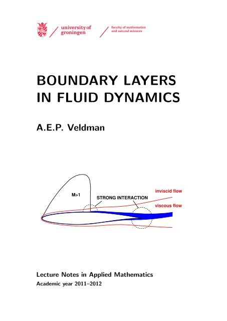
<strong>BOUNDARY</strong> <strong>LAYERS</strong><br />
<strong>IN</strong> <strong>FLUID</strong> <strong>DYNAMICS</strong><br />
A.E.P. Veldman<br />
M>1<br />
STRONG <strong>IN</strong>TERACTION<br />
inviscid flow<br />
viscous flow<br />
Lecture Notes in Applied Mathematics<br />
Academic year 2011–2012
<strong>BOUNDARY</strong> <strong>LAYERS</strong><br />
<strong>IN</strong> <strong>FLUID</strong> <strong>DYNAMICS</strong><br />
Code: WIBL-03<br />
Academic year: 2011–2012<br />
MSc Applied Mathematics<br />
MSc Mathematics<br />
Lecturer: A.E.P. Veldman<br />
University of Groningen<br />
Institute for Mathematics and Computer Science<br />
P.O. Box 407<br />
9700 AK Groningen<br />
The Netherlands
iii<br />
PROLOGUE<br />
It all started in 1904 at the International Mathematical Congress in Heidelberg, when Ludwig<br />
Prandtl give a lecture entitled “Über Flüssigkeitsbewegungen bei sehr kleiner Reibung” (English:<br />
“On fluid flow with very little friction”). He explained that the viscosity of a fluid plays<br />
a role in a (very) thin layer adjacent to the surface, which he called “Uebergangsschicht” or<br />
“Grenzschicht”. Translated into English, the latter led to the term boundary layer. With this<br />
lecture, the understanding of fluid flow was significantly increased. For instance, d’Alembert’s<br />
Paradox, stating that a body placed in a potential flow does not experience a force – clearly<br />
in conflict with every-day experience – was resolved. Subsequently, it could be explained,<br />
e.g., why birds and airplanes can fly. The thus far invisible boundary layer was responsible.<br />
Finally, as a spin-off, a new branch of mathematics was created: singular perturbation theory.<br />
In these lecture notes we will have a closer look at the flow in boundary layers. At various<br />
levels of modeling the featuring physical phenomena will be described. Also, numerical<br />
methods to solve the equations of motion in the boundary layer are discussed. Outside the<br />
boundary layer the flow can be considered inviscid (i.e. non viscous). The overall flow field<br />
is found by coupling the boundary layer and the inviscid outer region. The coupling process<br />
(both physically and mathematically) will also receive ample attention.<br />
It is recommended to have some basic knowledge of fluid dynamics and numerical methods<br />
for solving partial differential equations, for instance from the RuG lectures on Fluid<br />
Dynamics, Numerical Mathematics and/or Computational Fluid Dynamics.<br />
Groningen, Spring 2012
Contents<br />
1 THE <strong>BOUNDARY</strong>-LAYER EQUATIONS 1<br />
1.1 The Navier–Stokes equations . . . . . . . . . . . . . . . . . . . . . . . . . . . 2<br />
1.2 The boundary-layer approximation . . . . . . . . . . . . . . . . . . . . . . . . 4<br />
1.3 Influence of boundary layer on external flow . . . . . . . . . . . . . . . . . . . 10<br />
1.4 Similarity solutions . . . . . . . . . . . . . . . . . . . . . . . . . . . . . . . . . 14<br />
2 TURBULENT FLOW 19<br />
2.1 Structure of a turbulent boundary layer . . . . . . . . . . . . . . . . . . . . . 19<br />
2.2 Reynolds-averaged equations . . . . . . . . . . . . . . . . . . . . . . . . . . . 23<br />
2.3 Turbulence models . . . . . . . . . . . . . . . . . . . . . . . . . . . . . . . . . 25<br />
3 <strong>IN</strong>TEGRAL FORMULATION 31<br />
3.1 The Von Kármán equation . . . . . . . . . . . . . . . . . . . . . . . . . . . . . 31<br />
3.2 History of solution methods . . . . . . . . . . . . . . . . . . . . . . . . . . . . 33<br />
3.3 Problems near flow separation . . . . . . . . . . . . . . . . . . . . . . . . . . . 37<br />
3.4 The normal pressure gradient . . . . . . . . . . . . . . . . . . . . . . . . . . . 37<br />
4 ASYMPTOTIC PO<strong>IN</strong>T OF VIEW 39<br />
4.1 Classical boundary-layer theory . . . . . . . . . . . . . . . . . . . . . . . . . . 39<br />
4.2 Strong interaction and the triple deck . . . . . . . . . . . . . . . . . . . . . . 42<br />
5 NUMERICAL SOLUTION METHODS 49<br />
5.1 Parabolic character . . . . . . . . . . . . . . . . . . . . . . . . . . . . . . . . . 49<br />
5.2 The heat equation - numerical . . . . . . . . . . . . . . . . . . . . . . . . . . . 50<br />
5.3 The boundary-layer equations – numerical . . . . . . . . . . . . . . . . . . . . 55<br />
6 FLOW SEPARATION 59<br />
6.1 Something goes wrong . . . . . . . . . . . . . . . . . . . . . . . . . . . . . . . 59<br />
6.2 Asymptotic theory and numerical approach . . . . . . . . . . . . . . . . . . . 60<br />
6.3 A numerical experiment . . . . . . . . . . . . . . . . . . . . . . . . . . . . . . 62<br />
7 COUPL<strong>IN</strong>G OF <strong>BOUNDARY</strong> LAYER AND EXTERNAL FLOW 65<br />
7.1 Coupling algorithms . . . . . . . . . . . . . . . . . . . . . . . . . . . . . . . . 65<br />
7.2 Formulation of a model problem . . . . . . . . . . . . . . . . . . . . . . . . . 67<br />
7.3 Discretisation of the external flow . . . . . . . . . . . . . . . . . . . . . . . . . 68<br />
7.4 Numerical analysis of the model problem . . . . . . . . . . . . . . . . . . . . . 70<br />
7.5 Further analysis of the quasi-simultaneous method . . . . . . . . . . . . . . . 73<br />
v
vi<br />
CONTENTS<br />
7.6 Appendices . . . . . . . . . . . . . . . . . . . . . . . . . . . . . . . . . . . . . 76<br />
7.6.1 Appendix 1: Matrix prerequisites . . . . . . . . . . . . . . . . . . . . . 76<br />
7.6.2 Appendix 2: Generalization to other disciplines . . . . . . . . . . . . . 76<br />
8 OTHER EQUATIONS OF MOTION 79<br />
8.1 Parabolised Navier–Stokes equations . . . . . . . . . . . . . . . . . . . . . . . 79<br />
8.2 General discretisation principles . . . . . . . . . . . . . . . . . . . . . . . . . . 81<br />
8.3 Appendix: Some functional analysis . . . . . . . . . . . . . . . . . . . . . . . 82
Chapter 1<br />
THE <strong>BOUNDARY</strong>-LAYER<br />
EQUATIONS<br />
As Prandtl showed for the first time in 1904, usually the viscosity of a fluid only plays a<br />
role in a thin layer (along a solid boundary, for instance). Prandtl called such a thin layer<br />
“Uebergangsschicht” or “Grenzschicht”; the English terminology is boundary layer or shear<br />
layer (Dutch: grenslaag).<br />
In this first chapter Prandtl’s theory will be described, and the equations of motion that<br />
are valid in such a boundary layer are presented. As a starting point, the equations capable<br />
to describe the flow of any fluid (liquid or gas) are taken: the Navier–Stokes equations.<br />
The large influence of the boundary layer is<br />
visible in the accompanying illustrations. Here<br />
the solution is shown of two computations of<br />
flow past an RAE 2822 airfoil: a ‘viscous’ computation<br />
with boundary layer and an ‘inviscid<br />
= non-viscous’ computation without boundary<br />
layer. (In computer simulation it is very easy<br />
to switch certain physical effects on and off; in<br />
an experiment that is usually more difficult. . . )<br />
It is clear 1 that the lift (Dutch: draagkracht)<br />
of the wing is significantly lowered by the presence<br />
of the boundary layer. The adjacent figure<br />
also shows a comparison with experiment 2 .<br />
The most important reason for the difference<br />
between theory and experiment, visible as a<br />
difference in shock position, is the uncertainty<br />
in turbulence modeling.<br />
1 Lift is generated by a difference in pressure between upper and lower side: it equals the surface area<br />
between the upper and lower curve in the plot.<br />
2 The difference between theory and experiment in the pressure distribution at the leading edge of the airfoil<br />
is caused by a small discrepancy between the shape of the scale model that was actually used in the wind<br />
tunnel experiments and the intended airfoil shape as used in the computations.<br />
1
2 CHAPTER 1. THE <strong>BOUNDARY</strong>-LAYER EQUATIONS<br />
Inviscid computation<br />
Viscous computation<br />
1.1 The Navier–Stokes equations<br />
The motion of a continuous medium can be described by kinematic and dynamic conservation<br />
laws for mass, momentum and energy, extended with thermodynamical equations of state.<br />
These will be formulated in terms of independent variables in space x = (x 1 , x 2 , x 3 ) t and in<br />
time t. The dependent variables are denoted as<br />
velocity vector u = (u 1 , u 2 , u 3 ) t ,<br />
density ρ,<br />
pressure p,<br />
internal energy e,<br />
temperature T .<br />
The equations are presented in conservation form for a Cartesian coordinate system. Differentiation<br />
with respect to the i-th coordinate direction of a quantity φ is denoted as ∂ i φ.<br />
Further, the sommation convention for repeated indices is used.<br />
Conservation of mass<br />
Conservation of massa is described by the equation of continuity<br />
Conservation of momentum<br />
The momentum equation (Dutch: impulsvergelijking) reads<br />
∂ t ρ + ∂ i (ρu i ) = 0. (1.1)<br />
∂ t (ρu i ) + ∂ j (ρu i u j ) = ρF i + ∂ j σ ij . (1.2)<br />
F i is the i-component of an external force per unit of mass and volume; σ = (σ ij ) is the stress<br />
tensor. The stress tensor describes the force acting on the interface between fluid elements.<br />
It consists of a component perpendicular to the interface (normal stress) and a component<br />
in the interface (shear stress). In an inviscid medium only the normal stress exists, which is<br />
termed pressure; in a viscous medium additional terms are present, which together form the<br />
viscous stress tensor τ. Whence<br />
σ ij = −p δ ij + τ ij , (1.3)
1.1. THE NAVIER–STOKES EQUATIONS 3<br />
with δ ij the Kronecker symbol. In a so-called Newtonian medium the viscous stress tensor<br />
is linearly proportional to the velocity gradient. For a medium in local thermodynamic<br />
equilibrium this leads to the following model for τ:<br />
τ ij = 2µ(e ij − 1 3 e kkδ ij ), (1.4)<br />
where<br />
e ij = 1 2 (∂ ju i + ∂ i u j )<br />
is the deformation tensor, and µ the dynamical or molecular viscosity.<br />
The above equations (1.2), with the stress tensor formulated according to (1.3) and (1.4),<br />
are the factual Navier–Stokes equations: presented by Navier in 1823 and (independently) by<br />
Stokes in 1845. In every-day practice, the name also covers the continuity equation (1.1) and<br />
the energy equation (1.5).<br />
Conservation of energy<br />
Conservation of total energy E = e + 1 2 u iu i can be formulated as<br />
∂ t (ρE) + ∂ i (ρEu i ) = ρF i u i + ∂ j (u i σ ij ) − ∂ i q i . (1.5)<br />
In the right-hand side two terms can be recognized describing the work done by the external<br />
and internal forces, and a term featuring the heat flux q i . For many fluids, the heat flux is<br />
proportional to the temperature gradient (Fourier’s law)<br />
q i = −k ∂ i T. (1.6)<br />
Equations of state<br />
The above set of equations has to be closed with two thermodynamic equations of state. For<br />
an ideal gas these read<br />
p = ρRT and e = c v T. (1.7)<br />
R = c p − c v , with c p and c v the specific heats. The latter usually are assumed to be constant.<br />
Finally, the dependence of µ and k depend on the state of the fluid has to be specified, in<br />
particular on the temperature T .<br />
The equations (1.1), (1.2) and (1.5) are valid for each viscous, heat conducting fluid.<br />
The equations (1.3), (1.4), (1.6) and (1.7) make more specific statements about the fluid.<br />
When µ = 0 and k = 0 (i.e. no viscosity and no heat conduction) the Euler equations arise,<br />
formulated by Euler already in 1755.<br />
Incompressible formulation<br />
When the fluid is incompressible, i.e. when its density ρ is constant, the equations of motion<br />
can be simplified. The continuity equation becomes<br />
∂ i u i = 0, (1.8)
4 CHAPTER 1. THE <strong>BOUNDARY</strong>-LAYER EQUATIONS<br />
and the momentum equation now reads<br />
∂ t u i + ∂ j (u i u j ) = F i + 1 ρ ∂ jσ ij . (1.9)<br />
When also the viscosity µ is assumed constant, these two equations are sufficient to describe<br />
the flow. The temperature can be obtained from the following version of the energy equation<br />
∂ t (c v T ) + ∂ j (c v T u j ) = 1 ρ ∂ i(k ∂ i T ) + 2µ e ij ∂ j u i . (1.10)<br />
The above equations have to be supplied with boundary conditions. Along a solid boundary<br />
the velocity component perpendicular to the boundary has to be zero; for a viscous fluid<br />
also the tangential velocity has to vanish (no-slip condition). Further, along the boundary<br />
the temperature can be prescribed or its normal derivative (adiabatic boundary). At in- and<br />
outflow boundaries other conditions do apply (see the CFD lecture notes).<br />
By expanding the stress tensor σ ij in (1.9), and by using (1.8), the Navier–Stokes equations<br />
for an incompressible fluid can be written as<br />
∂u<br />
∂t + (u · grad) u = F − 1 ρ<br />
Here the kinematic viscosity ν = µ/ρ has been introduced.<br />
div u = 0, (1.11)<br />
grad p + ν div grad u. (1.12)<br />
When an internal flow is simulated, without in- or outflow openings, i.e. in a domain Ω<br />
with solid boundary Γ, at the boundary only a condition for the velocity u can be formulated.<br />
As indicated above, usually this condition will be<br />
u = 0 along Γ. (1.13)<br />
1.2 The boundary-layer approximation<br />
The Navier–Stokes equations are considered sufficiently general to describe the Newtonian<br />
fluids appearing in hydro- and aerodynamics. The solution of these equations is a complex<br />
job, also with computational means (despite the fast computers available nowadays). Fortunately,<br />
the equations contain terms that can be neglected in large parts of the flow domain.<br />
This allows the equations to be simplified, and herewith to reduce the effort for solving them.<br />
The terms that describe the viscous shear stresses offer such a possibility for simplification.<br />
These terms are only of interest in local areas of high shear (boundary layer, wake).<br />
Outside these areas ‘non-viscous’ equations can be used.<br />
We begin with the derivation of the equations that describe the flow in shear layers, like<br />
boundary layers and wakes. Starting point are the Navier–Stokes equations for steady, twodimensional,<br />
incompressible flow, where the density ρ is assumed constant. The equations<br />
are formulated in a Cartesian coordinate system (x, y) with velocity components (u, v). It is<br />
further assumed that the x-axis coincides (locally) with the solid boundary.
1.2. THE <strong>BOUNDARY</strong>-LAYER APPROXIMATION 5<br />
The equations of motion for steady two-dimensional incompressible flow are<br />
∂u<br />
∂x + ∂v<br />
⎫<br />
∂y = 0,<br />
u ∂u<br />
∂x + v ∂u<br />
(<br />
∂y = −1 ∂p ∂ 2 )<br />
ρ ∂x + ν u<br />
∂x 2 + ∂2 u<br />
⎪⎬<br />
∂y 2 ,<br />
u ∂v<br />
∂x + v ∂v<br />
(<br />
∂y = −1 ∂p ∂ 2 )<br />
ρ ∂y + ν v<br />
∂x 2 + ∂2 v<br />
∂y 2 .<br />
⎪⎭<br />
(1.14)<br />
Along a solid surface the velocity satisfies (u, v) = (0, 0). The second condition<br />
v = 0 at a solid surface<br />
(1.15a)<br />
also holds for non-viscous flow. The first condition<br />
u = 0 at a solid surface<br />
(1.15b)<br />
only holds for viscous flow. This is the no-slip condition, and prevents the shear stress at the<br />
wall to become infinite. When the flow is studied at a molecular level this condition has to<br />
be adapted; in practice this is only relevant for highly rarefied gases.<br />
Estimates outside the boundary layer<br />
Next a global estimate of the order of magnitude of the various terms in the Navier–Stokes<br />
equations is derived. Firstly, we will study the flow field not too close to the body surface. In<br />
such a situation the flow contains a length scale L determined by the geometry of the body;<br />
for an airfoil the chord length would be characteristic. Not too close to the body it may be<br />
assumed that variations in flow variables will only appear on this length scale.<br />
✻<br />
✛<br />
L<br />
✲<br />
characteristic length<br />
✲<br />
distance<br />
Further, as a velocity scale the problem possesses the magnitude of the oncoming flow U ∞ .<br />
Any variations in velocity will also be of that order. In this way, derivatives of the velocity<br />
can roughly be estimated according to<br />
∂u<br />
∂x ∼ U ∞<br />
L ;<br />
similar for the other first-order derivatives. Hence, in the continuity equation both terms are<br />
of equal importance.
6 CHAPTER 1. THE <strong>BOUNDARY</strong>-LAYER EQUATIONS<br />
In the x-momentum equation the convective terms can be estimated as<br />
u ∂u<br />
∂x ∼ U ∞<br />
2<br />
L<br />
(the other term is equally large),<br />
and the diffusive terms as<br />
The ratio between these two types of terms is<br />
ν ∂2 u<br />
∂x 2 ∼ ν U ∞<br />
L 2 .<br />
convection<br />
diffusion<br />
∼ U ∞L<br />
ν<br />
≡ Re, (1.16)<br />
the Reynolds number (Dutch: Reynoldsgetal). This ratio holds in areas where L is the characteristic<br />
length scale. The y-momentum equation can be treated in a similar fashion.<br />
When the Reynolds number is large, outside the boundary layer the Navier–Stokes equations<br />
can be simplified to the Euler equations<br />
u ∂u<br />
∂x + v ∂u<br />
∂y = −1 ρ<br />
u ∂v<br />
∂x + v ∂v<br />
∂y = −1 ρ<br />
∂p<br />
⎫⎪<br />
∂x , ⎬<br />
(1.17)<br />
∂p<br />
∂y . ⎪ ⎭<br />
This system requires less boundary conditions than Navier–Stokes. As a consequence, one of<br />
the boundary conditions from (1.15a, 1.15b) has to be dropped. Obviously, this should be the<br />
condition caused by the viscosity, as we have removed the viscosity from the mathematical<br />
model. Hence, along a solid wall only the condition<br />
v = 0 (normal velocity)<br />
may be prescribed. In general, the tangential velocity will not be zero. Therefore, along a solid<br />
boundary an Euler solution will usually not satisfy the boundary conditions for Navier–Stokes.<br />
Apparently, the Navier–Stokes solution becomes quite different from the Euler solution, at<br />
least in the neighborhood of the boundary. With this reasoning, heuristically the presence<br />
of a boundary layer close to the wall can be motivated. In this layer, the flow will possess<br />
another length scale, namely the distance to the wall. Now the above reasoning has to be<br />
reconsidered.<br />
Examples: For many flows the Reynolds number is very large, for example the flow of air<br />
around a car or an airplane, or the flow of water around a ship. The following table shows<br />
the coefficients of viscosity for air and water (at 15 ◦ C and 1 atm).<br />
ρ (kg/m 3 ) µ (kg/m sec) ν (cm 2 /sec)<br />
air 1.225 1.78 · 10 −5 1.45 · 10 −5<br />
water 0.9991 · 10 3 1.137 · 10 −3 1.138 · 10 −6<br />
It follows that air is over 10 times as viscous as water! For a number of applications this<br />
yields the following Reynolds numbers:
1.2. THE <strong>BOUNDARY</strong>-LAYER APPROXIMATION 7<br />
medium char. vel. char. length Re<br />
cyclist (tourist) air 15 km/h 0.5 m 1 · 10 5<br />
golf ball (pro) air 200 km/h 0.04 m 2 · 10 5<br />
speed skater (pro) air 45 km/h 0.8 m 5 · 10 5<br />
swimmer (pro) water 5 km/h 1.5 m 2 · 10 6<br />
car air 120 km/h 4 m 1 · 10 7<br />
shark water 20 km/h 4 m 2 · 10 7<br />
airplane (wing) air 900 km/h 3 m 5 · 10 7<br />
ship water 20 km/h 200 m 1 · 10 9<br />
Estimates inside the boundary layer<br />
In the boundary layer, the tangential velocity of the Euler solution has to be brought back<br />
to zero at the wall.<br />
u<br />
✲<br />
✻<br />
y, v<br />
✻<br />
δ<br />
❄<br />
✲<br />
x, u<br />
Let us now try to estimate the thickness of this boundary layer. For simplicity we will<br />
consider the boundary layer along a straight boundary, coinciding with the x-axis. First, our<br />
assumptions will be made more precise:<br />
1. the velocity at the outer edge of the boundary layer is of the order U;<br />
2. the derivatives in x-direction can be estimated by means of a characteristic length L<br />
that is independent of ν;<br />
3. the thickness of the boundary layer has a characteristic size δ with δ ≪ L; derivatives<br />
in y-direction can be based upon this length scale;<br />
4. no external influence exists (like e.g. a shock wave) that introduces a special scale for<br />
the pressure gradient; the pressure gradient adapts to the other terms in the equations.<br />
The estimations start with the continuity equation<br />
∂u<br />
∂x + ∂v<br />
∂y = 0.<br />
The first term ∂u/∂x ∼ U/L, which then should also hold for the second term ∂v/∂y. At the<br />
surface v = 0, which implies that inside the boundary layer<br />
v ∼ δU L .
8 CHAPTER 1. THE <strong>BOUNDARY</strong>-LAYER EQUATIONS<br />
Next the x-momentum equation is considered<br />
We conclude:<br />
u ∂u<br />
∂x + v ∂u = − 1 ∂p<br />
∂y ρ ∂x + ν ∂2 u<br />
∂x<br />
} {{ }<br />
2 + ν ∂2 u<br />
} {{ } ∂y 2 .<br />
} {{ }<br />
U 2<br />
νU<br />
L<br />
L 2 νU<br />
δ 2<br />
• both convective terms are equally large ∼ U 2 /L;<br />
• the diffusive term with the x-derivatives is much smaller than that with the y-derivatives;<br />
• the largest of the diffusive terms balances with the convective terms when<br />
U 2<br />
L ∼ νU<br />
δ 2<br />
Finally, the momentum equation in y-direction is considered<br />
⇒ δ<br />
L ∼ √ ν<br />
UL = Re−1/2 . (1.18)<br />
u ∂v<br />
∂x + v ∂v = − 1 ∂p<br />
∂y ρ ∂y + ν ∂2 v<br />
∂x<br />
} {{ }<br />
2 + ν ∂2 v<br />
} {{ } ∂y 2 .<br />
} {{ }<br />
U 2 δ<br />
νUδ<br />
L 2<br />
L 3 νU<br />
δL<br />
The convective term and the diffusive term in y-direction are equally important, ∼ U 2 δ/L 2 ,<br />
and this determines the order of magnitude of ∂p/∂y. The pressure variation across the<br />
boundary layer becomes ∼ ρU 2 δ 2 /L 2 . The x-momentum equation yields the pressure itself<br />
to be ∼ ρU 2 . Hence, in first approximation, the pressure can be considered constant in the<br />
y-direction.<br />
When these estimates are substituted in the Navier–Stokes equations, the following system<br />
of equations is left<br />
∂u<br />
∂x + ∂v<br />
∂y = 0,<br />
⎫⎪ ⎬<br />
u ∂u<br />
∂x + v ∂u<br />
∂y = −1 ∂p<br />
ρ ∂x + ν ∂2 u<br />
∂y 2 ,<br />
(1.19)<br />
0 = − 1 ∂p<br />
ρ ∂y . ⎪ ⎭<br />
These are the boundary-layer equations (Dutch: grenslaagvergelijkingen), with which the flow<br />
in a shear layer can be approximately described. The corresponding boundary conditions are<br />
at the surface (y = 0) : u = v = 0 ;<br />
at the edge (y = y e ) : u = u e , p → p e ,<br />
(1.20)<br />
where u e and p e follow from the inviscid Euler solution. The index ‘e’ stems from the word<br />
’edge’ (Dutch: rand). Herewith, at the outer boundary the tangential velocity at the surface
1.2. THE <strong>BOUNDARY</strong>-LAYER APPROXIMATION 9<br />
from the Euler flow (which would not vanish) is prescribed. From the Euler equation (1.17)<br />
at the surface, where v = 0, it follows<br />
du e<br />
u e<br />
dx = −1 ∂p e<br />
ρ ∂x , (1.21)<br />
and this form of Bernoulli’s equation can be substituted in (1.19). Then the x-momentum<br />
equation becomes<br />
u ∂u<br />
∂x + v ∂u<br />
∂y = u du e<br />
e<br />
dx + ν ∂2 u<br />
∂y 2 . (1.22)<br />
Next we will analyze the mathematical character of the system (1.19)+(1.22). Hereto it<br />
is reformulated as a first-order system by introducing ∂u/∂y = ω:<br />
⎛<br />
0 1 0<br />
⎞ ⎛<br />
⎝ v 0 −ν ⎠ ⎝<br />
}<br />
1 0<br />
{{<br />
0<br />
}<br />
A<br />
u<br />
v<br />
ω<br />
⎞<br />
⎠<br />
y<br />
⎛<br />
+ ⎝<br />
1 0 0<br />
u 0 0<br />
0 0 0<br />
} {{ }<br />
B<br />
⎞ ⎛<br />
⎠ ⎝<br />
u<br />
v<br />
ω<br />
⎞<br />
⎠<br />
x<br />
=<br />
⎛<br />
⎜<br />
⎝<br />
0<br />
u e<br />
du e<br />
dx<br />
ω<br />
The characteristic directions λ = dx/dy follow from det(λA − B) = 0. This results in a<br />
3-fold root λ = 0, with characteristic direction x = Constant. This situation cannot be fully<br />
labelled along theoretical lines. When v ≡ 0, (1.22) shows a parabolic character with stable<br />
direction x → ∞ for u > 0; for u < 0 this direction switches. We will come back to this<br />
later. This consideration suggests that, for u > 0, the x-direction is a time-like direction, and<br />
that the system can be solved by a ‘marching’ process in x-direction. As initial condition<br />
the velocity profile of u has to be prescribed upstream (only ∂u/∂x appears in the equation;<br />
∂v/∂x is not present). This is in contrast to the full Navier–Stokes equations which also<br />
⎞<br />
⎟<br />
⎠
10 CHAPTER 1. THE <strong>BOUNDARY</strong>-LAYER EQUATIONS<br />
do require boundary conditions downstream. The steady Navier–Stokes equations possess a<br />
partly elliptic character through their diffusive terms. But also without diffusion, i.e. Euler,<br />
the acoustical part of the equation (div u & grad p) provides an elliptic character (see PDV<br />
lecture notes - Veldman 1996). It will be clear that the boundary-layer equations can be<br />
solved much more easily than Navier–Stokes and Euler.<br />
Not alone in the boundary layer, but in more parts of the flow domain the Navier–Stokes<br />
equations can be simplified. Outside the boundary layer the Euler equations are valid. These<br />
are essential when strong shocks appear in the flow, because in the shock rotation is generated.<br />
For weak shocks the flow can be modeled as a potential flow (which is irrotational). In the<br />
above figure, the subdivision of the flow field according to the relevant modeling is shown;<br />
such a subdivision is termed zonal modeling.<br />
1.3 Influence of boundary layer on external flow<br />
Because the boundary layer is very thin, in first instance this suggests to compute the external<br />
flow around the ‘clean’ body, i.e. without boundary layer. Based on the external streamwise<br />
velocity, thereafter the boundary layer can be computed. Finally, the external flow has to be<br />
corrected for the presence of the boundary layer.<br />
Displacement thickness<br />
The effect of the boundary layer on the external flow is expressed in a quantity called displacement<br />
thickness (Dutch: verdringingsdikte), denoted by δ ∗ . Via the no-slip condition,<br />
the streamwise velocity in the boundary layer is smaller than it would have been in an inviscid<br />
flow. As a consequence, the transport of mass also becomes smaller. The displacement<br />
thickness denotes how much the wall has to be shifted for an inviscid flow past the displaced<br />
wall to have the same mass transport as the viscous flow along the original wall, i.e.<br />
y u e ✲<br />
✻<br />
✁<br />
✁ ✁<br />
✁✁ ✁<br />
✁<br />
✁ ✁ ✁ ✁ ✁ ✁✁ ✁ ✻ <br />
<br />
δ ∗ <br />
<br />
<br />
❄<br />
u ✲<br />
∫ ye<br />
0<br />
u(x, y) dy =<br />
∫ ye<br />
δ ∗<br />
u e (x) dy,<br />
where y e is chosen sufficiently large (there u ≈ u e<br />
should hold). As a consequence, in the adjacent figure,<br />
where u has been plotted as a function of y, the<br />
shaded areas have the same surface area. By rewriting<br />
the above definition we find<br />
δ ∗ (x) = 1<br />
u e (x)<br />
∫ ∞<br />
0<br />
{u e (x) − u(x, y)} dy. (1.23)<br />
δ ∗ gives the modified shape of the body as it is experienced by the external flow: the body<br />
looks thicker because of the lower velocities in the boundary layer.<br />
This can be further explained by considering the vertical velocity in the boundary layer.<br />
The continuity equation gives<br />
∂v<br />
∂y = −∂u ∂x .
1.3. <strong>IN</strong>FLUENCE OF <strong>BOUNDARY</strong> LAYER ON EXTERNAL FLOW 11<br />
As u = u e at the edge of the boundary layer, it can be expected that v grows linearly according<br />
to v ∼ −y du e /dx. The next term in the series expansion of v for large y is the interesting<br />
one. Suppose<br />
then we have<br />
v(x, y) ∼ − du e<br />
dx y + v 1(x) + · · · , y → ∞,<br />
[<br />
v 1 (x) = lim v(x, y) + du ]<br />
e<br />
y→∞<br />
dx y [∫ y<br />
∂v<br />
= lim<br />
y→∞<br />
0 ∂y (x, y) dy + du ]<br />
e<br />
dx y [∫ y<br />
= lim − ∂u<br />
y→∞<br />
0 ∂x (x, y) dy + du ]<br />
e<br />
dx y [∫ y<br />
{ due<br />
= lim<br />
y→∞<br />
0 dx − ∂u } ]<br />
∂x (x, y) dy<br />
= d ∫ ∞<br />
(u e − u) dy ≡ d<br />
dx<br />
dx (u eδ ∗ ). (1.24)<br />
At the outer edge of the boundary layer the vertical velocity behaves like<br />
0<br />
v(x, y) ∼ − du e<br />
dx y + d<br />
dx (u eδ ∗ ), y → ∞. (1.25)<br />
To have a smooth match with the external flow, this also has to hold for the vertical velocity<br />
of the external flow close to the wall. In more detail we must have<br />
In first instance we had chosen this expression to be zero.<br />
v EIF (x, 0) ≈ d<br />
dx (u eδ ∗ ). (1.26)<br />
v<br />
✻<br />
viscous v<br />
(RVF)<br />
❅❘<br />
<br />
❅■ v EIF (x, 0)<br />
RVF = real viscous flow<br />
EIF = extrapolated inviscid flow<br />
❅❅■ extrapolated inviscid v (EIF)<br />
y<br />
✲<br />
In the above interpretation, the presence of the boundary layer can be formulated as a<br />
transpiration velocity through the surface. An alternative formulation states that the displacement<br />
body is a streamline of the external flow. This immediately follows from the expansion<br />
of v given in (1.25). Choose y = δ ∗ , and note that high in the boundary layer u ≈ u e , then<br />
we have<br />
v(x, δ ∗ ) ≈ − du e<br />
dx δ∗ + d<br />
dx (u eδ ∗ dδ ∗<br />
) = u e<br />
dx ,
12 CHAPTER 1. THE <strong>BOUNDARY</strong>-LAYER EQUATIONS<br />
such that<br />
stating that y = δ ∗ is a streamline.<br />
v<br />
u (x, δ∗ ) ≈ dδ∗<br />
dx , (1.27)<br />
In Chapter 4 we will formulate the above heuristics in terms of singular perturbation<br />
theory.<br />
Momentum thickness<br />
Next to an equation based on mass transport, we also can compare the viscous and inviscid<br />
flow based on momentum transport. Thus, the momentum thickness (Dutch: impulsverliesdikte)<br />
is defined as the additional distance (compared to the δ ∗ ) over which the wall has to<br />
be displaced such that an inviscid flow produces the same momentum transport:<br />
∫ ye<br />
δ ∗ +θ<br />
u 2 e dy =<br />
∫ ye<br />
0<br />
u 2 dy.<br />
Herewith we have<br />
θ = 1 u 2 e<br />
∫ ∞<br />
0<br />
(u 2 e − u 2 ) dy − δ ∗ = 1 u 2 e<br />
∫ ∞<br />
0<br />
u(u e − u) dy. (1.28)<br />
This quantity is related to the drag caused by the boundary layer, as shown next.<br />
D<br />
✻<br />
C<br />
U ∞ ✲<br />
boundary-layer edge<br />
h<br />
A<br />
❄<br />
B<br />
Consider the above control volume and monitor the conservation of momentum in x-<br />
direction, i.e. conservation of ρu. The increase in momentum has to be caused by external<br />
forces. Such forces are generated by the pressure and by the viscous (shear/normal) stresses.<br />
We obtain<br />
∂<br />
∂t<br />
∫<br />
V<br />
∫<br />
ρu dV +<br />
S<br />
∫<br />
ρu u n dS = (σ · n) x dS, (1.29)<br />
with σ the stress tensor and (σ · n) x the x-component of the force exerted on a surface with<br />
normal n.<br />
S
1.3. <strong>IN</strong>FLUENCE OF <strong>BOUNDARY</strong> LAYER ON EXTERNAL FLOW 13<br />
For incompressible flow we have<br />
σ ij = −p δ ij + µ (∂ j u i + ∂ i u j ),<br />
which describes the i-component of the force per surface unit acting on a surface element with<br />
normal in the j-direction. In our analysis we are only interested in the forces in x-direction.<br />
Changing the notation gives<br />
σ xx = −p + 2µ ∂u<br />
∂x , σ xy = µ<br />
( ∂u<br />
∂y + ∂v )<br />
.<br />
∂x<br />
In steady equilibrium, in (1.29) the ∂/∂t-term drops out, and we are left with<br />
∫<br />
∫<br />
∫<br />
ρu 2 dS + ρuv dS − ρu 2 dS =<br />
BC<br />
DC<br />
AD<br />
∫<br />
= − µ ∂u<br />
AB ∂y<br />
∫BC<br />
dS + (−p + 2µ ∂u<br />
( ∂u<br />
∂x<br />
∫DC<br />
) dS + µ<br />
∂y + ∂v ) ∫<br />
dS + (p − 2µ ∂u<br />
∂x<br />
AD ∂x ) dS,<br />
where we have used already that v = 0 at the surface. Further, in the viscous terms the<br />
contribution of µ ∂u/∂y at the surface dominates because ∂u/∂y is larger than ∂u/∂x. Also<br />
the contributions from the pressure cancel, because in a Blasius flow the pressure is constant.<br />
Finally, when the other viscous contributions are neglected, the following relation remains<br />
∫<br />
BC<br />
∫<br />
ρu 2 dS +<br />
DC<br />
∫<br />
ρuv dS −<br />
AD<br />
∫<br />
ρu 2 dS = −<br />
AB<br />
µ ∂u<br />
∂y dS ≡ −D B.<br />
The right-hand side equals the drag (Dutch: weerstand) D that the flow experiences due the<br />
viscous forces (shear stress - Dutch: schuifspanning) along the surface up to the point B.<br />
AD is chosen far enough upstream such that u = U ∞ , the oncoming flow. Along the plate<br />
u e = U ∞ . Further, CD is chosen high enough such that u ≈ U ∞ , but v is not zero (the flow<br />
has to make way due to the displacement effect). We are left with<br />
∫ h<br />
∫<br />
D B = ρ(U∞ 2 − u 2 ) dy − U ∞ ρv dx.<br />
0<br />
From mass conservation for the control volume information can be obtained on the behavior<br />
of v along the upper side<br />
∫<br />
∫<br />
∫<br />
∫<br />
∫ h<br />
ρu dS + ρv dS − ρu dS = 0 =⇒ ρv dS = ρ(U ∞ − u) dy.<br />
BC<br />
DC<br />
Substituting this results in<br />
D B = ρ<br />
AD<br />
∫ h<br />
0<br />
DC<br />
DC<br />
u(U ∞ − u) dy evaluated at B,<br />
where without problems we can let h → ∞ since u approaches U ∞ = u e sufficiently fast.<br />
Recognizing the definition of the momentum thickness (1.28), the drag of the plate (upto the<br />
point B) can be written as<br />
D B = ρU 2 ∞θ(B). (1.30)<br />
0
14 CHAPTER 1. THE <strong>BOUNDARY</strong>-LAYER EQUATIONS<br />
Skin-friction coefficient<br />
We have just encountered the shear stress along the surface. This quantity is often denoted<br />
by<br />
τ w ≡ µ ∂u<br />
∂y ∣ . (1.31)<br />
wall<br />
The corresponding non-dimensional coefficient is called the skin-friction coefficient (Dutch:<br />
schuifspanningscoëfficiënt)<br />
c f ≡<br />
τ w<br />
1<br />
. (1.32)<br />
2 ρu2 e<br />
As we just saw, the shear stress produces the viscous contribution to the drag.<br />
1.4 Similarity solutions<br />
To find ‘analytical’ solutions of partial differential equations, like the boundary-layer equations,<br />
often similarity solutions are sought. Inspired by the method of separation of variables,<br />
it is hoped to find solutions with a similarity structure. For the boundary-layer equations we<br />
look for velocity profiles that are the same at each x-station apart from a scaling (in space<br />
and/or in magnitude):<br />
u(x, y) = u e (x) f ′ (η) with η = y/L(x).<br />
This will be substituted in (1.22) to find out whether there exist special choices of u e (x) which<br />
allow for such a similarity solution.<br />
First, the streamfunction is introduced<br />
Ψ(x, y) ≡<br />
∫ y<br />
with which the vertical velocity is given by<br />
u e f ′ ( due<br />
dx f ′ + u e f<br />
0<br />
u dy = u e (x)L(x)f(η),<br />
v(x, y) = − ∂Ψ<br />
∂x = − d<br />
dx (u eL) f(η) − u e L f ′ (η) ∂η<br />
∂x .<br />
Substitution in the x-momentum equation gives<br />
)<br />
−<br />
which can be rewritten as<br />
u e<br />
du e<br />
dx<br />
′′ ∂η<br />
∂x<br />
( d<br />
dx (u eL) f + u e L f ′ ∂η<br />
∂x<br />
)<br />
ue<br />
L f ′′ = u e<br />
du e<br />
dx + ν u e<br />
L 2 f ′′′ ,<br />
(<br />
(f ′ ) 2 − ff ′′) − u2 e dL du e<br />
L dx ff′′ = u e<br />
dx + ν u e<br />
L 2 f ′′′ . (1.33)<br />
If we would succeed to divide the x-dependency out of the equation, then an ordinary differential<br />
equation in only one independent variable η is obtained. This will be successful<br />
when<br />
du e<br />
u e<br />
dx ∼ u2 e dL<br />
L dx ∼ ν u e<br />
L 2 .
1.4. SIMILARITY SOLUTIONS 15<br />
It simply can be verified that the choice<br />
√ ν<br />
u e ∼ U x p , L ∼<br />
U xq with q = 1 2<br />
(1 − p) (1.34)<br />
satisfies the above condition. Recognize in L the proportionality with Re −1/2 deduced earlier.<br />
The inviscid velocity u e from (1.34) corresponds<br />
with flow past a wedge (Dutch: wig). To show<br />
this, using conformal mapping, we will calculate<br />
the potential past a wedge with full opening angle<br />
βπ . When the wedge lies in a complex z-<br />
plane, then the conformal mapping<br />
−ζ = (−z) 2<br />
2−β (1.35)<br />
maps this wedge onto the positive real axis<br />
in the ζ-plane. The −-signs in this map are<br />
necessary to position the cuts along the positive<br />
real axis (i.e. inside the wedge).<br />
y<br />
❆❑ x<br />
❆❆✟ ✟✟ ✟✯<br />
❆❑ βπ/2<br />
✟<br />
❍<br />
✟✟✟✟✟✟✟✟✟✟✟<br />
❄<br />
❍<br />
❍<br />
❍<br />
❍<br />
❍<br />
❍<br />
❍<br />
❍<br />
❍<br />
❍<br />
❍<br />
The complex velocity potential χ corresponding to the flow along the flat plate in the<br />
ζ-plane is χ = Uζ. In the z-plane, the corresponding complex velocity potential is obtained<br />
from substitution of the conformal mapping (1.35). Hence<br />
χ = −(−z) 2<br />
2−β U<br />
describes the flow past the wedge 3 . The velocity field follows from dχ/dz (we need only its<br />
absolute velocity):<br />
|u| = |u − iv| =<br />
dχ<br />
∣ dz ∣ = 2U<br />
2 − β |z| β<br />
2−β .<br />
Falkner–Skan equation<br />
Thus the streamwise velocity along the surface of the wedge is given by (note x = |z| is the<br />
distance from the nose)<br />
u e (x) = U x β/(2−β) . (1.36)<br />
Herewith, we have obtained the required form of u e for the existence of similarity solutions<br />
of the boundary-layer equations. Via p = β/(2 − β) and q = 1 2<br />
(1 − p) = (1 − β)/(2 − β), see<br />
(1.34), we arrive at<br />
√<br />
u(x, y) = u e (x) f ′ U<br />
(η) with η =<br />
ν(2 − β) x(β−1)/(2−β) y, (1.37)<br />
where the scale factor in η has been chosen such that (1.38) becomes simpler. From (1.33) it<br />
follows that the function f(η) satisfies the Falkner–Skan equation (1930)<br />
f ′′′ + ff ′′ + β ( 1 − (f ′ ) 2) = 0, f(0) = f ′ (0) = 0, f ′ (∞) = 1. (1.38)<br />
3 Since the streamfunction Ψ = Im χ = 0 for ζ along the positive real axis, the streamfunction also vanishes<br />
when z lies on the wedge ⇒ the wedge is a streamline.
16 CHAPTER 1. THE <strong>BOUNDARY</strong>-LAYER EQUATIONS<br />
This equation does not possess a solution for all β. Nowadays (i.e. since the late 1970’s) we<br />
know that this property is related to the problems that are encountered in boundary layers<br />
featuring flow separation.<br />
When 0 ≤ β ≤ 1 a unique solution exists, in which f ′ → 1 exponentially for η → ∞. When<br />
β ∗ ≡ −0.1988 · · · < β < 0 two solutions exist with this property. One of these solutions has<br />
f ′′ (0) > 0, while for the other solution f ′′ (0) < 0. The latter solution shows backflow (Dutch:<br />
terugstroming), i.e. it features an area where f ′ (η) < 0. The figure above gives a sketch of<br />
the corresponding streamline patterns; the figure below shows the velocity profiles.<br />
The latter figure also shows two other important quantities: f ′′ (0) which is related to the<br />
shear stress, and δ ≡ ∫ ∞<br />
0 (1 − f ′ (η))dη = lim {η − f(η)} which is related to the displacement<br />
η→∞<br />
thickness. When −1 ≤ β < β ∗ no exponentially decaying solutions exist, whereas for |β| > 1<br />
an abundance of solutions exists (Oskam & Veldman 1982; Botta et al. 1986). Which role<br />
these solutions play in practice is still unclear. Through (1.36) the parameter β is linked to<br />
the velocity gradient (pressure gradient):<br />
Flat plate<br />
β<br />
2 − β = x u e<br />
du e<br />
dx . (1.39)<br />
An important special case is β = 0, corresponding with flow past a flat plate. This case is<br />
named after Blasius, who discussed it in 1908. The streamwise velocity of the potential flow<br />
is simply constant u e = U. The coordinate transformation (1.37) gives<br />
√<br />
U<br />
η = y<br />
2xν . (1.40)<br />
Thus the thickness of the boundary layer grows proportional to √ x.
1.4. SIMILARITY SOLUTIONS 17<br />
The velocity profile u = Uf ′ (η) satisfies the Blasius equation<br />
f ′′′ + ff ′′ = 0, f(0) = f ′ (0) = 0, f ′ (∞) = 1.<br />
Its solution, experimentally observed, is shown above. Important values are f ′′ (0) = 0.4696<br />
and δ = 1.217. The skin friction coefficient becomes<br />
c f = µ<br />
∂u<br />
1<br />
2 ρU 2 ∂y ∣ = µ<br />
√ √ √ U ∂u<br />
2ν<br />
ν<br />
1<br />
y=0 2 ρU 2 2xν ∂η ∣ =<br />
η=0<br />
xU f ′′ (0) = 0.664<br />
xU ,<br />
and the displacement thickness<br />
δ ∗ = 1 U<br />
∫ ∞<br />
0<br />
(U − u) dy =<br />
√<br />
2xν<br />
U<br />
∫ ∞<br />
0<br />
(1 − f ′ ) dη =<br />
√<br />
2xν<br />
U δ.<br />
Often, by lack of another length scale, a Reynolds number is introduced based on the distance<br />
from the leading edge<br />
Re x = Ux<br />
ν .<br />
In terms of this Reynolds number we can write<br />
c f = 0.664 Re −1/2<br />
x and δ ∗ = 1.721 x Re −1/2<br />
x . (1.41)
18 CHAPTER 1. THE <strong>BOUNDARY</strong>-LAYER EQUATIONS<br />
The momentum thickness is given by<br />
θ = 1 ∫ ∞<br />
√ ∫ 2xν ∞<br />
U 2 u(U − u) dy =<br />
f ′ (1 − f ′ ) dη<br />
0<br />
U 0<br />
√ √<br />
2xν<br />
2xν<br />
=<br />
U [f − ff′ − f ′′ ] ∞ 0 =<br />
U f ′′ (0) = 0.664 x Rex −1/2 . (1.42)
Chapter 2<br />
TURBULENT FLOW<br />
For not too large Reynolds numbers the flow looks smooth. The streamlines are nicely parallel<br />
to each other, as in thin layers (Greek: lamina). We call this laminar flow. For larger Reynolds<br />
numbers such a flow becomes unstable for disturbances. As a result the flow appears much<br />
more irregular: turbulent flow. Below a snapshot of a turbulent boundary layer is shown.<br />
Both the laminar and the turbulent parts of the flow can be seen very clearly.<br />
2.1 Structure of a turbulent boundary layer<br />
The seemingly chaotic behavior of turbulent flow enhances the exchange of momentum in<br />
comparison with laminar flow. Since the shear stress is directly proportional, it is relatively<br />
large in turbulent shear layers. The larger momentum transport makes turbulent velocity<br />
19
20 CHAPTER 2. TURBULENT FLOW<br />
profiles much fuller than laminar velocity profiles. The wall shear stress is larger, resulting in<br />
a larger drag.
2.1. STRUCTURE OF A TURBULENT <strong>BOUNDARY</strong> LAYER 21<br />
Typical velocity profiles for laminar and turbulent flow along a flat plate are shown in<br />
the first of the above figures (taken from Moran 1984). The other figure shows the wall<br />
shear stress as a function of the distance to the leading edge (non-dimensional Re x ). For<br />
Re>≈ 3 × 10 5 the flow can become turbulent, with its corresponding larger c f . The laminar<br />
solution of Blasius has been discussed in §1.4. The transition from laminar to turbulent flow<br />
takes place in a transition process to which we return in §2.3.<br />
The velocity profile of a turbulent boundary layer is quite different from that of a laminar<br />
boundary layer (see preceding section). We will have a close look at it now. In a turbulent<br />
boundary layer often three regions (layers) are distinguished:<br />
• an outer layer (Dutch: buitenlaag) which is sensitive to the properties of the external<br />
flow;<br />
• an inner layer (Dutch: binnenlaag) where turbulent mixing is the dominant physics;<br />
• a laminar sublayer (Dutch: laminaire sublaag) close to the surface where the turbulent<br />
stresses are negligible with respect to µ ∂u/∂y (the no-slip condition implies u ′ = v ′ = 0<br />
at the surface).<br />
These layers naturally blend into each other (sometimes the blending region between laminar<br />
sublayer and inner layer is called buffer zone). The figure above shows a velocity profile,<br />
plotted against a logarithmic scale in y (be aware!) which shows the inner layers much
22 CHAPTER 2. TURBULENT FLOW<br />
thicker than they actually are. The profile has been made non-dimensional with the friction<br />
velocity (Dutch: wrijvingssnelheid)<br />
u τ ≡ √ τ w /ρ, (2.1)<br />
in which τ w is the shear stress along the surface.<br />
Laminar sublayer<br />
In the laminar sublayer the shear stress is dominated by the molecular contribution τ =<br />
µ ∂u/∂y. As this layer is very thin, τ cannot be much different from its value at the wall τ w .<br />
Hence in this layer we have approximately<br />
Combining this with (2.1) yields<br />
u ≈ τ w<br />
µ y.<br />
u + ≡ u u τ<br />
≈ ρu τ y<br />
µ ≡ y+ . (2.2)<br />
Observe that y + is a Reynolds number based on u τ and the distance to the wall. This quantity<br />
is plotted horizontally in the graph.<br />
Inner layer<br />
In the inner layer it is assumed that turbulent mixing is so important that properties of the<br />
external flow (outside the boundary layer) do not have influence. In that case, only one<br />
velocity scale can be made with the available parameters, namely √ τ/ρ. As characteristic<br />
value we take u τ , as defined in (2.1). To estimate the slope of the velocity profile we need<br />
a length scale l that is characteristic is for the mixing process. We call l the mixing length<br />
(Dutch: mengweglengte), and obtain as an estimate<br />
∂u<br />
∂y ≈ u τ<br />
l . (2.3)<br />
In the boundary layer only one length scale is available, namely the distance to the wall y.<br />
The mixing length is therefore chosen proportional to this distance:<br />
with κ a non-dimensional constant. Now<br />
which can be integrated to<br />
l ≡ κy, (2.4)<br />
∂u<br />
∂y = u τ<br />
κy ,<br />
u<br />
u τ<br />
= 1 κ ln y + C′ .<br />
Introducing C ′ = κ −1 ln(ρu τ /µ) + C, and using the notation from (2.2) the standard form of<br />
the law-of-the-wall (Dutch: wandwet) is obtained<br />
u + ≡ u u τ<br />
= 1 κ ln y+ + C. (2.5)
2.2. REYNOLDS-AVERAGED EQUATIONS 23<br />
This formula fits experimental data very well for κ = 0.41 and C = 5.0, as shown clearly<br />
in the above graph. The constant κ is named after Theodore Von Kármán (1930). The<br />
velocity profiles in the laminar sublayer (2.2) and in the inner layer (2.5) match continuously<br />
in y + ≈ 11.<br />
Outer layer<br />
In the outer layer the wall profile has to be adapted such that for large y it obtains a shape<br />
that ‘smoothly’ approaches u e . This profile has to be dependent of the y-coordinate scaled<br />
by the boundary-layer thickness, i.e. y/δ(x). For small y the adaptation should be small, say<br />
∼ y 2 . This gave Coles (1956) the idea to use a ‘sin 2 y’-function. He suggested the following<br />
velocity profile, which turns out to fit many experimental data<br />
u + = 1 κ ln y+ + C + 2 ( ) πy<br />
κ Π(x) sin2 , y ≤ δ(x). (2.6)<br />
2δ(x)<br />
This velocity profile is also very useful in the inner layer, where y/δ(x) is small. For y = δ(x)<br />
the velocity has to match the external flow, which yields<br />
u e<br />
= 1 u τ κ ln δu τ<br />
ν + C + 2 Π. (2.7)<br />
κ<br />
In total we now have three unknowns u τ , δ and Π. One equation has been given in (2.7),<br />
two more equations are needed. These will be derived from the equations of motion; more on<br />
this subject in Chapter 3.<br />
2.2 Reynolds-averaged equations<br />
Turbulent flow still can be described by the equations of motion from Chapter 1. These<br />
equations do allow solutions with a very small length scale and time scale. To describe these<br />
phenomena with a discrete numerical method, very fine computational grids with very small<br />
time steps are required. This is impossible with the current performance of computers. Therefore,<br />
the influence of the small-scaled phenomena on the larger scales, which can be resolved<br />
by the grid, is usually described by a turbulence model.<br />
Osborne Reynolds was the first who, around 1890, followed such an approach. He assumed<br />
a clear distinction in time scale between the local turbulent phenomena and the more global<br />
phenomena in the flow. This allows to divide the variables into a mean value and a fluctuation.<br />
For instance<br />
u = ū + u ′ , p = ¯p + p ′ , (2.8)<br />
in which ū is the mean value of u over a time interval T that is small with respect to the<br />
global time scale but large w.r.t. the turbulent time scale:<br />
ū(x, t) = 1 T<br />
∫ t+T<br />
t<br />
u(x, τ) dτ. (2.9)<br />
For the incompressible case we will elaborate this a bit. Substitute (2.8) in (1.8)+(1.9)<br />
and integrate these equations between t and t + T . As approximately ∫ t+T<br />
t<br />
u ′ dτ = 0, by
24 CHAPTER 2. TURBULENT FLOW<br />
definition of ū, the terms that are linear in u and p do not contribute from u ′ of p ′ . Only the<br />
convective term ∂ j (u i u j ) provides a source for the appearance of u ′ . The following system of<br />
equations emanates<br />
∂ i ū i = 0,<br />
Here the Reynolds stress tensor<br />
∂ t ū i + ∂ j (ū i ū j ) + ∂ j R ij = ¯F i + 1 ρ ∂ j ¯σ ij . (2.10)<br />
R ij = u ′ i u′ j + u′ iūj + ū i u ′ j<br />
(2.11)<br />
has been introduced. It stems from the convective terms, but it has the appearance of a<br />
stress tensor; therefore it is usually combined with the stress tensor σ ij . Subsequently some<br />
approximations are introduced. When ū i and ū j are constant over the integration interval<br />
(t, t + T ) the following expressions are valid<br />
u ′ iūj = 0, ū i u ′ j = 0, ū iū j = ū i ū j and ∂ t ū i = ∂ t ū i . (2.12)<br />
In general (2.12) only holds approximately. After substitution of (2.12) in (2.10) the Reynoldsaveraged<br />
Navier–Stokes (RaNS) equations follow<br />
∂ i ū i = 0,<br />
∂ t ū i + ∂ j (ū i ū j ) = ¯F i + ∂ j<br />
( 1<br />
ρ ¯σ ij + ˜R ij<br />
)<br />
(2.13)<br />
where ˜R ij = −u ′ i u′ j .<br />
The problem with solving these time-averaged Navier–Stokes equations are the new unknowns<br />
u ′ i , for which in first instance no equation is available. Finding such an equation<br />
is called the closure problem (Dutch: sluitingsproblem). This is the essence of turbulence<br />
modeling: ˜Rij has to be expressed in known quantities like ū and ¯p. More on this in §2.3.<br />
The estimation of the magnitude of the Reynolds stresses proceeds somewhat different<br />
than in §1.2. There – with change of notation u = (u, v) – v ≪ u, but for the fluctuations<br />
u ′ and v ′ this does not hold; in general u ′ and v ′ will be of equal magnitude. The Reynolds<br />
stresses u ′ v ′ , u ′2 and v ′2 are all three equally large. But, as before, y-derivatives will be larger<br />
than x-derivatives, hence simplification is possible. Often the following terms are left in the<br />
boundary-layer approximation:<br />
ū ∂ū ∂ū<br />
+ ¯v<br />
∂x ∂y = −1 ρ<br />
∂ ¯p<br />
∂x + ∂ ( µ<br />
∂y ρ<br />
)<br />
∂ū<br />
∂y − u′ v ′ , (2.14a)<br />
0 = − 1 ∂ ¯p<br />
ρ ∂y + ∂ ( )<br />
µ ∂¯v<br />
∂y ρ ∂y − v′2 . (2.14b)<br />
The most important term neglected in the x-momentum equation (2.14a) is ∂(u ′2 )/∂x which<br />
is a factor δ/L smaller than the term ∂(u ′ v ′ )/∂y (in laminar flow the factor between both<br />
diffusive terms is δ 2 /L 2 ). In the y-momentum equation (2.14b) we sometimes retain part of<br />
the diffusive term. The Reynolds stress part learns that ∂ ¯p/∂x and ∂ ¯p/∂y are comparable.<br />
But since y is small, the pressure variation in vertical direction is of lower order than ¯p itself;<br />
therefore ∂ ¯p/∂y = 0 is still often used.
2.3. TURBULENCE MODELS 25<br />
2.3 Turbulence models<br />
We will now return to the contribution of u ′ v ′ in the x-momentum equation (2.14a).<br />
equation has to be found which describes this contribution: the closure problem.<br />
An<br />
One way is to multiply the Navier–Stokes equations with u or v. Then expressions are<br />
formed of the products of velocities, but with 3 velocity factors, à la (u ′ ) 2 v ′ . Subsequently<br />
we have to come up with something for this kind of terms. In other words: this is replacing<br />
one problem with another.<br />
The more brisk way is to directly produce formulas for u ′ v ′ that reasonably match experimental<br />
data. Hereto, first it is assumed that the turbulent events are proportional to velocity<br />
differences in the boundary layer. By observing that the Reynolds stress tensor R ij appearing<br />
in (2.13) is similar to the stress tensor σ ij , a Boussinesq-type suggestion is made<br />
Thus the following closure relation is assumed<br />
R ij = ɛ(∂ j u i + ∂ i u j ).<br />
−u ′ v ′ ≡ ɛ ∂u<br />
∂y , (2.15)<br />
where ɛ is called the eddy viscosity. The name stems from the larger structures in turbulent<br />
flow, which are called ‘eddies’ (Dutch: draaikolken). In this way the shear stress, see (2.14a),<br />
can be approximated as<br />
τ = µ ∂u<br />
∂y − ρu′ v ′ ≈ (µ + ρɛ) ∂u<br />
∂y . (2.16)<br />
The quantity ɛ has dimension velocity × length. Therefore it is written as<br />
ɛ = v t l, (2.17)<br />
with v t a velocity scale to be chosen, and l the mixing length from §2.1.<br />
Cebeci-Smith model<br />
The simple algebraic turbulence models choose for v t Prandtl’s mixing length model (1925)<br />
v t = l<br />
∂u<br />
∣ ∂y ∣ . (2.18)<br />
Together with (2.17) this results in<br />
∣ ∣∣∣<br />
ɛ = l 2 ∂u<br />
∂y ∣<br />
met l = κy. (2.19)<br />
In the sublayer this model does not work satisfactory. Therefore, Van Driest (1956) proposed<br />
to change the expression for l into<br />
(<br />
l = κy 1 − e −y+ /A +) , (2.20)
26 CHAPTER 2. TURBULENT FLOW<br />
with, as before, y + = yu τ /ν, u τ = √ τ w /ρ and A + = 26. For small y + (2.20) reduces the<br />
value of l with respect to the original expression; this is plausible since next to the wall less<br />
length is available for the mixing. Also in the outer layer, ɛ is often modified; for example as<br />
ɛ = 0.0168 u e δ ∗ . (2.21)<br />
ɛ<br />
u e δ ∗<br />
0.0168<br />
✻<br />
Eddy viscosity according to Cebeci-Smith<br />
y<br />
✲<br />
The equations (2.19)-(2.21) form the eddy-viscosity model of Cebeci–Smith (1967, 1974),<br />
much used in aerodynamics where the bodies often are very slender.<br />
k − ɛ model<br />
Of course, it is very well possible to choose quite something different for v t in (2.17). We<br />
will discuss such a model, that is especially being used in hydrodynamics: the k − ɛ model<br />
(Launder & Spalding 1972). In this model, first the turbulent kinetic energy is introduced:<br />
k = 1 2 u′ i u′ i .<br />
For k a transport equation is postulated. Such a transport equation consists of a convective<br />
part, a dissipative part and, sometimes, a production part (source term).<br />
In boundary-layer approximation the equation for k usually looks like<br />
u ∂k<br />
∂x + v ∂k ∣ ∣∣∣ ∂u<br />
2<br />
= ν t ∂y ∂y ∣ − ɛ + ∂ (<br />
ν + ν )<br />
t ∂k<br />
,<br />
∂y σ<br />
} {{ } } {{ }<br />
k ∂y<br />
} {{ }<br />
convection production diffusion<br />
with ν t = c µ k 2 /ɛ, and ɛ the dissipation of the kinetic energy.<br />
For ɛ also an equation has to be found. Unfortunately, physical insight hardly gives any<br />
clues; many versions exist. We describe one popular version in boundary-layer approximation<br />
[<br />
u ∂ɛ<br />
∂x + v ∂ɛ ∣ ]<br />
∣∣∣<br />
∂y = ∂u<br />
2<br />
c ɛ1 ν t ɛ<br />
∂y ∣ − c ɛ2 ɛ<br />
k + ∂ [(<br />
ν + ν ) ]<br />
t ∂ɛ<br />
.<br />
∂y σ ɛ ∂y<br />
This equation has been chosen such that its mathematical structure is similar to that of the<br />
k-equation. The free constants usually are chosen as<br />
c µ = 0.09, c ɛ1 = 1.44, c ɛ2 = 1.92, σ k = 1, σ ɛ = 1.3.
2.3. TURBULENCE MODELS 27<br />
Both equations require boundary conditions at the surface and at the outer edge. At the surface,<br />
based on the behavior as described in §2.1 a wall function for k and ɛ can be formulated<br />
in the inner layer. As boundary condition for the equations continuity is required of k and ɛ<br />
at the transition from inner and outer layer (near y + ≈ 11). At the outer edge again many<br />
variants are possible: the simplest is k = ɛ = 0 as y → ∞.<br />
Many other turbulence models have been formulated. An overview can be found e.g. on<br />
the webpage www.cfd-online.com/Wiki/Turbulence modeling.<br />
Transition<br />
At the end of this chapter on turbulent flow we close with some remarks on the transition from<br />
laminar to fully turbulent flow. This transition is triggered when a laminar flow is no longer<br />
able to damp disturbances; loosely spoken, ‘the boundary layer gets exhausted’ (Dutch: ’de<br />
grenslaag raakt vermoeid’). This is due to the decelerating influence of the wall.<br />
Stability analysis of the boundary-layer equations is limited since the equations are nonlinear.<br />
Models that describe transition do exist, but they are very approximate. Much more<br />
urgent than for the modelling of turbulence, direct simulations, with their required resolution<br />
in space and time, are necessary to create more insight in the transition behavior.<br />
The ‘grand challenge’<br />
It must be stressed that the modeling of turbulence and transition is the most important<br />
problem in flow simulation. It will remain challenging for many years to come; we give an<br />
impression of its current status.<br />
For attached (Dutch: aanliggend) flow the situation is most optimistic; most turbulence<br />
models give good results (at fixed transition). However, often the flow features recirculation<br />
zones, e.g. behind sluice gates and breakwaters, behind buildings and hart valves, behind<br />
cars, ships and airplanes, in combustion chambers and cooling systems, etc. For these applications<br />
still no turbulence models exist that can provide flow simulations with the accuracy<br />
as requested by industry.<br />
As an example we discuss the flow around airplane wings during take-off and landing,<br />
where (due to the low air speed) the lift coefficient has to be as large as possible. According<br />
to potential-flow theory, the lift increases proportional with the angle of attack (Dutch:
28 CHAPTER 2. TURBULENT FLOW<br />
invalshoek). However, viscous effects, in particular the decambering (Dutch: ontwelving) of<br />
the profile due to the displacement effects of the boundary layer, lead to a smaller increase<br />
in lift. Even, at a certain angle of attack the lift starts to decrease, around the moment that<br />
massive (trailing-edge) separation sets in. Also, the drag of the profile is rising sharply. The<br />
graph below (taken from Torenbeek & Wittenberg 2002) shows the behaviour of lift and drag<br />
with increasing angle-of-attack. It will be clear that the value of maximum lift is one of the<br />
most essential parameters in wing design; the flow behaviour in separated flow regions plays<br />
a crucial role here.<br />
The uncertainty in turbulence modeling for this situation is currently larger than the difference<br />
between the boundary-layer approximation and the full Navier–Stokes equations. As<br />
an illustration we show in the α − C L plane (angle-of-attack versus lift) a number of computations<br />
for the RAE 2822 profile under conditions near maximum lift. The graph shows a<br />
0.86<br />
0.82<br />
0.78<br />
0.74<br />
✻<br />
x<br />
+<br />
+<br />
+<br />
+<br />
+<br />
+ +<br />
x<br />
x ◦<br />
+<br />
x<br />
x<br />
✲<br />
α<br />
RAE 2822 - Case 10<br />
M ∞ = 0.750<br />
Re = 6.2 × 10 6<br />
+ Navier-Stokes<br />
x boundary-layer meth.<br />
◦ experiment (corr.)<br />
C L<br />
2.40 2.60 2.80 3.00
2.3. TURBULENCE MODELS 29<br />
close-up of the situation around point B in the above figure (although another airfoil is involved).<br />
In 1987, this flow case was the subject of a workshop (Holst 1987), in which various<br />
Navier–Stokes and boundary-layer methods participated. The figure also shows an experimental<br />
result. All Navier–Stokes computations are close together, but they predict a lift that<br />
is too high. The boundary-layer methods, however, come closer to the experiment. Most of<br />
the latter methods make use of an integral formulation (see Chapter 3), in which the flow is<br />
modeled in an ‘engineering’ way.<br />
Therefore, at this moment it is not yet worthwhile in airplane design to apply the more<br />
than 100× as expensive Navier–Stokes methods. In the future, when our knowledge of turbulence<br />
has increased sufficiently, this will change undoubtedly. It is expected that extremely<br />
expensive direct numerical simulations, with sufficient resolution of all space and time scales,<br />
are necessary to design better turbulence models. Finding such models, necessary to keep the<br />
calculation times acceptable for industrial applications, is one of the ‘Grand Challenges’ of<br />
modern science and engineering.<br />
The above challenge has been envisioned already by Sir Horace Lamb in 1932, then aged<br />
83, when he stated in a speech to the British Association for the Advancement of Science:<br />
I am an old man now, and when I die and go to heaven there are two matters on<br />
which I hope for enlightenment. One is quantum electrodynamics, and the other<br />
is the turbulent motion of fluids. And about the former I am rather optimistic.<br />
According to another apocryphal story, Werner Heisenberg was asked what he would ask<br />
God, given the opportunity. His reply was:<br />
When I meet God, I am going to ask him two questions: Why relativity And why<br />
turbulence I really believe he will have an answer for the first.<br />
The situation has not changed significantly since then (see e.g. Speciale & So 1998).
30 CHAPTER 2. TURBULENT FLOW
Chapter 3<br />
<strong>IN</strong>TEGRAL FORMULATION<br />
3.1 The Von Kármán equation<br />
In the time that solving partial differential equations was in its infancy, people have been<br />
looking for more global descriptions of the flow. For the description of a boundary layer,<br />
formulations have been sought which average in vertical direction. In this way, ordinary<br />
differential equations in streamwise direction are left; but of course we loose flow details in<br />
normal direction.<br />
The x-momentum equation (1.22) can be rewritten as<br />
∂<br />
∂x (u2 ) + ∂ ∂y (uv) = u du e<br />
e<br />
dx + 1 ∂τ<br />
ρ ∂y . (3.1)<br />
This equation is integrated between y = 0 and y = h, where we will specify the outer edge<br />
later:<br />
∫ h<br />
∂<br />
h<br />
∂x (u2 ) dy + uv<br />
du e<br />
∣ = u e<br />
dx h + τ h<br />
ρ ∣ . (3.2)<br />
0<br />
The vertical velocity at the outer edge is found from the continuity equation<br />
v∣ h =<br />
0<br />
∫ h<br />
0<br />
0<br />
∫<br />
∂v<br />
h<br />
∂y dy = − ∂u<br />
∂x dy.<br />
At the wall y = 0 we have u = v = 0 and τ = τ w . When h is chosen outside the boundary<br />
layer, then u = u e and τ = 0. Substitution hereof in (3.2) leads to<br />
∫ h<br />
0<br />
∫<br />
∂<br />
h<br />
∂u<br />
∂x (u2 ) dy − u e<br />
∂x dy = u du e<br />
e<br />
dx h − τ w<br />
ρ .<br />
The pressure gradient is shifted to the left-hand side<br />
∫ h<br />
0<br />
0<br />
∫<br />
∂<br />
h<br />
∂x (u2 − u 2 ∂<br />
e) dy − u e<br />
∂x (u − u e) dy = − τ w<br />
ρ .<br />
The integrands decay fast enough when y → ∞, and the ∂/∂x is moved outside the integral.<br />
Then we arrive at<br />
d<br />
dx<br />
∫ ∞<br />
0<br />
(u 2 e − u 2 ) dy − u e<br />
d<br />
dx<br />
0<br />
31<br />
∫ ∞<br />
0<br />
0<br />
(u e − u) dy = τ w<br />
ρ ,<br />
0
32 CHAPTER 3. <strong>IN</strong>TEGRAL FORMULATION<br />
which can be rewritten via the definitions from §1.3 as<br />
d [<br />
u<br />
2<br />
dx e (θ + δ ∗ ) ] d<br />
− u e<br />
dx (u eδ ∗ ) = τ w<br />
ρ .<br />
Finally we expand all differentiations and divide by u 2 e. Then we obtain<br />
dθ<br />
dx + θ u e<br />
(2 + H) du e<br />
dx = 1 2 c f , (3.3)<br />
in which<br />
H ≡ δ ∗ /θ<br />
is the shape factor (Dutch: vormfactor), and c f is the skin friction coefficient defined in §1.3.<br />
This momentum integral equation was introduced by Von Kármán in 1921.<br />
The equation contains a number of unknowns: θ, H and c f . To determine these two<br />
additional relations are required. These are constructed along many (creative) ways, of which<br />
we give an example.<br />
A possibility to create an extra equation is to multiply (3.1) with u and then to integrate.<br />
An equation based on the energy is then obtained. Using the continuity equation, the starting<br />
point is written as<br />
u 2 ∂u ∫ y<br />
∂x − u∂u ∂u<br />
∂y 0 ∂x dy − u u du e<br />
e<br />
dx = µ u<br />
ρ u∂2 ∂y 2 . (3.4)<br />
This equation is integrated with respect to y between 0 and h.<br />
left-hand side gives<br />
∫ h<br />
0<br />
[<br />
u ∂u ∫ y<br />
]<br />
∂u<br />
∂y 0 ∂x dy dy =<br />
∫ h ∫ y<br />
0<br />
0<br />
∂u<br />
∂x dy d( 1 2 u2 ) =<br />
The second term at the<br />
∫ y<br />
1<br />
2 u2 0<br />
∣<br />
∂u ∣∣∣<br />
h<br />
∂x dy<br />
0<br />
∫ h<br />
−<br />
0<br />
The first and the third term of (3.4) give together<br />
∫ h<br />
0<br />
[<br />
u 2 ∂u ]<br />
∂x − u u du e<br />
e dy = 1<br />
dx<br />
2<br />
1 ∂u<br />
2u2 ∂x dy = 1 2<br />
∫ h<br />
0<br />
∫ h<br />
0<br />
u ∂<br />
∂x (u2 − u 2 e) dy.<br />
(u 2 e − u 2 ) ∂u<br />
∂x dy.<br />
Together with a partial integration of the right-hand side of (3.4) this results in<br />
1<br />
2<br />
d<br />
dx<br />
∫ ∞<br />
0<br />
u(u 2 e − u 2 ) dy = µ ρ<br />
∫ ∞<br />
0<br />
( ) ∂u 2<br />
dy, (3.5)<br />
∂y<br />
where the limit h → ∞ has been taken. This is the energy integral equation.
3.2. HISTORY OF SOLUTION METHODS 33<br />
3.2 History of solution methods<br />
In the past - laminar<br />
Fist observe that the shape of a laminar velocity profile has quite smooth curves, resembling<br />
those of polynomials. Thus, the first calculations methods used simple polynomials<br />
to approximate the velocity profile u(x, y). Pohlhausen (1921) for example used a 4 ◦ -degree<br />
polynomial<br />
u<br />
= a + bη + cη 2 + dη 3 + eη 4 , η ≤ 1,<br />
u e<br />
with η = y/δ(x), in which δ(x) is the still unknown boundary-layer thickness. In total 6<br />
unknowns have to be solved from the following 6 equations<br />
at the surface: u = 0, u e<br />
du e<br />
dx = −ν ∂2 u<br />
∂y 2 ;<br />
at the edge: u = u e ,<br />
together with the Von Kármán integral equation.<br />
∂u<br />
∂y = 0, ∂ 2 u<br />
∂y 2 = 0;<br />
How fine this works will be shown with an even further simplified variant, in which only<br />
a 2 ◦ -degree polynomial is used<br />
u<br />
u e<br />
= a + bη + cη 2 ,<br />
η = y/δ(x).<br />
The coefficients follow from<br />
at the surface: u = 0;<br />
at the edge: u = u e and ∂u<br />
∂y = 0;<br />
resulting in<br />
By applying their definition, we find<br />
c f ≡ µ<br />
∂u<br />
1<br />
2 ρu2 e<br />
∂y ∣ = 4 ν<br />
y=0<br />
u e δ<br />
u<br />
= 2 y ( y<br />
) 2<br />
u e δ − , y ≤ δ.<br />
δ<br />
and<br />
θ ≡<br />
∫ δ<br />
Substitution hereof in the Von Kármán equation (3.3) yields<br />
0<br />
(<br />
u<br />
1 − u )<br />
dy = · · · = 2 u e u e 15 δ.<br />
2 dδ<br />
15 dx = 2ν<br />
u e δ<br />
with the solution<br />
δ 2 = 30 νx<br />
u e<br />
.<br />
It follows that<br />
c f = 0.73 Re −1/2<br />
x and θ = 0.73x Re −1/2<br />
x .<br />
The exact Blasius values differ less than 10%: the coefficient 0.73 should have been 0.664 (see<br />
(1.41) and (1.42)). One can imagine that use of a third- or fourth-order polynomial, which<br />
does require a bit more calculus, brings even better results (e.g. Kuethe & Schetzer 1950,<br />
Cebeci & Bradshaw 1977).
34 CHAPTER 3. <strong>IN</strong>TEGRAL FORMULATION<br />
In the past - turbulent<br />
The shape of turbulent velocity profile is quite different from a polynomial shape. Instead, for<br />
turbulent flow the velocity profile of Coles (2.6) are used. The three unknowns u τ , δ and Π<br />
follow from (2.7), the Von Kármán momentum integral equation (3.3) and the energy integral<br />
equation (3.5).<br />
The above methods perform not too bad for attached (Dutch: aanliggend) flow, but for<br />
separated (Dutch: losgelaten) flow the assumed velocity profiles (Pohlhausen’s polynomial or<br />
Coles’ profile) are not suited: they simply do not have the right kind of shape. Therefore,<br />
nowadays other methods are being used.<br />
Today – laminar<br />
For laminar flow a method is treated which performs quite well for separated flow. It is<br />
based on velocity profiles from the Falkner–Skan equation. This equation describes a family<br />
of solutions with one free parameter β. This family will be denoted by f β . The horizontal<br />
velocity is given by<br />
u<br />
= f β ′ (η) with η = y/L(x).<br />
u e<br />
The idea now is to consider β and the length scale L as two unknown functions of x, as in<br />
u<br />
= f<br />
β(x) ′ (y/L(x)) . (3.6)<br />
u e<br />
From this velocity profile the δ ∗ , θ, c f (and other quantities) can be expressed in terms of β(x)<br />
and L(x). Remains to find two equations for these two quantities. Hereto the Von Kármán<br />
momentum integral equation (3.3) and the energy integral equation (3.5) are selected.<br />
Today – turbulent<br />
Nowadays, the turbulent approach is no longer based on profile families. With more global<br />
considerations it is tried to derive some relations between the quantities θ, δ ∗ and c f , such<br />
that together with the momentum integral equation sufficient relations are available.<br />
A much-used method is the entrainment method of Head (1958), or refinements hereof.<br />
It is based on the following idea. Let δ(x) be the thickness of the boundary layer, then the<br />
mass transport is given by<br />
Q(x) =<br />
∫ δ(x)<br />
0<br />
u dy. (3.7)<br />
This quantity does not have to be constant, but usually increases significantly. An increase<br />
of Q has to be compensated by flow entering the boundary layer from outside. This flow<br />
E = dQ/dx<br />
is called entrainment velocity (Dutch literally: meeneemsnelheid).
3.2. HISTORY OF SOLUTION METHODS 35<br />
Comparing (3.7) with the definition of the displacement thickness we find<br />
δ ∗ = δ − Q/u e .<br />
Hence<br />
E = d<br />
dx u e(δ − δ ∗ ) ≡ d<br />
dx (u eθH 1 ), (3.8)<br />
where we have introduced<br />
H 1 ≡ δ − δ∗<br />
= δ − H. (3.9)<br />
θ θ<br />
With much entrained air, the behaviour of the boundary layer is highly influenced by it.<br />
Head’s idea is that properties of the entrained air are quite relevant for the global behaviour<br />
of the boundary layer. His first assumption is that the non-dimensional entrainment velocity<br />
E/u e only depends on H 1 . Based on several experiments, which are indicated in the left-hand<br />
graph below, the following relation was proposed (also indicated)<br />
1<br />
u e<br />
d<br />
dx (u eθH 1 ) = E u e<br />
= 0.0306 (H 1 − 3.0) −0.6169 . (3.10)<br />
The discrepancies between the experimental data and the above approximation do not really<br />
justify the amount of digits given, but in practice the original above formula is used.
36 CHAPTER 3. <strong>IN</strong>TEGRAL FORMULATION<br />
The second step is that Head assumes that H 1 can be expressed as a function of only<br />
the shape factor H = δ ∗ /θ. Head’s original experimental data and his fit are shown in the<br />
right-hand graph above. Note that his data only cover the range H ≤ 3, yet they do tend to<br />
indicate a minimum in the H-H 1 relation. In the 1980’s, more experiments have been carried<br />
out, and for this relation a number of variants have been proposed, some of them are shown<br />
graphically in (3.11). Indeed, the H-H 1 relation appears to show a minimum. Further analysis<br />
of the experimental data suggests that this minimum corresponds with the point of flow<br />
separation. In the next subsection we will demonstrate the dramatic impact of this minimum.<br />
(3.11)<br />
Finally, a relation for c f is required. In the original formulation of Head (1958) this is the<br />
Ludwig-Tillman formula<br />
with Re θ = u e θ/ν.<br />
c f = 0.246 × 10 −0.678H Re −0.268<br />
θ<br />
(3.12)<br />
The equations (3.10)-(3.12) + the Von Kármán equation (3.3) yield 4 equations for 4<br />
unknowns: θ, H, H 1 and c f .<br />
Relation (3.12) does not allow for negative values of c f , hence it is not very useful for<br />
separated flow. Therefore, in later years, this relation has been replaced by more complicated<br />
expressions, for example by Green (1972). Also (3.10) has been refined over the years. Chapter<br />
5 from Bradshaw (1976) gives more information.<br />
It should be realized that it has taken quite some trial-and-error effort and considerable<br />
insight to come up with combinations of parameters that appear to be more or less universal<br />
for boundary layers. This shows the craftmanship of the pioneers of applied fluid mechanics.<br />
Subsequently, it is quite remarkable that such a ‘crude’ engineering approach yields surprisingly<br />
good results for attached flow; even a limited amount of flow separation can be allowed.<br />
Navier–Stokes still has a hard time improving this approach (see the airfoil example at the<br />
end of Chapter 2).
3.3. PROBLEMS NEAR FLOW SEPARATION 37<br />
3.3 Problems near flow separation<br />
When the pressure gradient is positive, hence du e /dx negative, then the boundary layer<br />
decelerates. Forgetting ∂u/∂y and ∂ 2 u/∂y 2 for the moment, the boundary-layer equation<br />
reduces to<br />
u ∂u<br />
∂x = −1 ∂p<br />
ρ ∂x .<br />
The degree in which p increases is the same everywhere in the flow. Inside the boundary<br />
layer, where u is small, this has more effect than in its outer regions. After experiencing some<br />
unfavorable (positive) pressure gradient, negative velocities will appear in the boundary layer<br />
(backflow). The wall streamline has separated from the wall.<br />
The above system of equations starts to misbehave itself, which can be demonstrated by<br />
taking apart two equations, (3.8) and the Von Kármán equation. These are first reordered to<br />
Von Kármán:<br />
Entrainment:<br />
dθ<br />
dx<br />
= 1 2 c f − θ u e<br />
(2 + H) du e<br />
dx<br />
H 1<br />
dθ<br />
dx + θ dH 1<br />
dx = E u e<br />
− θH 1<br />
u e<br />
du e<br />
dx<br />
The other relations are of algebraic nature. The above relations form two differential equations<br />
from which θ and H 1 can be solved; the algebraic equations provide the other quantities.<br />
But now watch figure (3.11). The relation H − H 1 shows a minimum, hence not for every<br />
value H 1 a value for H can be found! In practice, this minimum is found to correspond with<br />
a point of flow separation (Dutch: loslaatpunt).<br />
Also the laminar approach breaks down. This is because not for all β a solution of the<br />
Falkner–Skan equation exists. The limiting value β = −0.1988 · · · corresponds with separating<br />
flow: f ′′ (0) = 0 (see §1.4).<br />
3.4 The normal pressure gradient<br />
In the boundary layer, in first instance the pressure is assumed constant in vertical direction.<br />
This assumption is not longer valid when the streamlines are highly curved. To understand<br />
this consider the inviscid part of the y-momentum equation<br />
u ∂v<br />
∂x + v ∂v<br />
∂y = −1 ρ<br />
The slope of a streamline is given by v/u. When the streamline runs more or less parallel to<br />
the x-axis, its curvature is approximately given by<br />
κ = d ( v<br />
)<br />
.<br />
dx u<br />
∂p<br />
∂y .<br />
Elementary calculus gives<br />
κ =<br />
u ∂v/∂x − v ∂u/∂x<br />
u 2 ,
38 CHAPTER 3. <strong>IN</strong>TEGRAL FORMULATION<br />
and using the continuity equation, the y-momentum equation can be rewritten as<br />
∂p<br />
∂y = −κρu2 .<br />
This holds for the viscous flow as well as for the inviscid external EIF (Equivalent Inviscid<br />
Flow). Their difference satisfies<br />
∂<br />
∂y (p EIF − p) = −κρ(u 2 EIF − u 2 ).<br />
At the outer edge of the boundary layer both pressures are equal. At the wall they become<br />
different<br />
∫ ∞<br />
p EIF,wall − p wall = κρ(u 2 EIF − u 2 ) dy.<br />
When u EIF is assumed constant, u EIF = u e , then we arrive at<br />
p EIF,wall − p wall = κρu2 e(θ + δ ∗ ).<br />
0<br />
The figure shows the difference between the real pressure<br />
and the extrapolated pressure from the external<br />
flow (for κ > 0). As the velocity in the boundary layer<br />
is smaller than that in the external flow, because<br />
∂p<br />
∣∂y<br />
∣ = |κρu2 | < |κρu 2 e| =<br />
∂p<br />
∣∂y<br />
∣ ,<br />
EIF<br />
the pressure through the boundary layer is more constant<br />
than the extrapolated pressure.<br />
y ✻<br />
y e<br />
0<br />
❏<br />
❏❏❏❏❏❏❏❏❏<br />
p<br />
p EIF<br />
✲<br />
p
Chapter 4<br />
ASYMPTOTIC PO<strong>IN</strong>T OF VIEW<br />
With small viscosity, the Navier–Stokes equations give rise to a singular perturbation problem.<br />
In this type of problems the perturbation parameter multiplies the highest-order derivative.<br />
In ‘classical’ perturbation problems, the solution can be written as a series expansion in<br />
the small parameter. In singular perturbation problems this can be done as well, but the<br />
domain where the problem is defined has to be divided in subdomains, in each of which other<br />
series expansions are valid. Usually, thin layers along boundaries are being split off. Following<br />
Prandtl, these layers are called boundary layers. The reason that along boundaries something<br />
different happens is because by zeroing the small parameter the highest order term is removed<br />
from the equation, and herewith also a boundary condition has to be removed. Hence, the<br />
zeroth-order solution does not satisfy all boundary conditions of the original problem, and<br />
this has to be repaired by adding a boundary layer.<br />
4.1 Classical boundary-layer theory<br />
We will reformulate our considerations from Chapter 1 in a way as is common for singular<br />
perturbation theory. Hereto, first non-dimensional variables are introduced<br />
¯x = x L , ȳ = y L , ū =<br />
u<br />
U ∞<br />
, ¯v =<br />
v<br />
U ∞<br />
, ¯p =<br />
p<br />
ρU 2 ∞<br />
. (4.1)<br />
With these scalings, the Navier–Stokes equations change into<br />
∂ū<br />
∂¯x + ∂¯v<br />
∂ȳ = 0,<br />
ū ∂ū ∂ū<br />
+ ¯v<br />
∂¯x ∂ȳ = − ∂ ¯p<br />
∂¯x + 1 Re<br />
ū ∂¯v ∂¯v<br />
+ ¯v<br />
∂¯x ∂ȳ<br />
= −∂<br />
¯p<br />
∂ȳ + 1 Re<br />
( )<br />
∂2ū<br />
∂¯x 2 + ∂2 ū<br />
∂ȳ 2 ,<br />
( ∂2¯v<br />
∂¯x 2 + ∂2¯v )<br />
∂ȳ 2 .<br />
⎫<br />
⎪⎬<br />
⎪⎭<br />
(4.2)<br />
The only difference with before is that the coefficient of the diffusion term has changed from<br />
ν into 1/Re. We will therefore omit the overbars; the diffusion coefficient will learn whether<br />
we are working with the non-dimensional or dimensional variables.<br />
39
40 CHAPTER 4. ASYMPTOTIC PO<strong>IN</strong>T OF VIEW<br />
As we saw in Chapter 1, the flow domain is divided in two parts: the boundary layer<br />
and the external flow region. In each of these domains the solution can be written in a series<br />
expansion. It is assumed that all terms in this expansion, including their derivatives,<br />
are bounded; if this is not the case then the expansion has to be reconsidered. Thereafter,<br />
this expansion is substituted in the equations of motion, and terms of equal powers in the<br />
perturbation parameter are taken together; here we use the boundedness of the terms.<br />
In Chapter 1 we already got an impression of the behavior of the solution. We saw that<br />
the small parameter ν plays a role through Re −1/2 . Therefore, first an expansion is postulated<br />
in integer powers of Re −1/2 .<br />
In the outer domain the asymptotic expansions become<br />
u(x, y; Re) = u E 0 (x, y) + Re−1/2 u E ⎫<br />
1 (x, y) + · · · , ⎬<br />
v(x, y; Re) = v0 E(x, y) + Re−1/2 v1 E (x, y) + · · · ,<br />
p(x, y; Re) = p E 0 (x, y) + Re−1/2 p E 1 (x, y) + · · · . ⎭<br />
(4.3)<br />
Substitution into the Navier–Stokes equations, and grouping the most important terms (i.e.<br />
Re 0 ) together reveals that u E 0 , vE 0 and pE 0 satisfy the Euler equations.<br />
In the boundary layer first a stretched coordinate in normal direction is introduced<br />
ỹ = Re 1 2 y. (4.4)<br />
This coordinate is O(1) in the boundary layer. The expansions in the boundary layer become<br />
u(x, y; Re) = u B 0 (x, ỹ) + Re−1/2 u B ⎫<br />
1 (x, ỹ) + · · · , ⎬<br />
v(x, y; Re) = Re −1/2 v0 B(x, ỹ) + Re−1 v1 B (x, ỹ) + · · · ,<br />
p(x, y; Re) = p B 0 (x, ỹ) + Re−1/2 p B 1 (x, ỹ) + · · · . ⎭<br />
(4.5)<br />
Substitution in Navier–Stokes shows that the leading terms satisfy the (non-dimensional form<br />
of the) boundary-layer equations<br />
∂u B 0<br />
∂x + ∂vB 0<br />
∂ỹ<br />
= 0,<br />
u B 0<br />
∂u B 0<br />
∂x + vB 0<br />
∂u B 0<br />
∂ỹ<br />
= − ∂pB 0<br />
∂x + ∂2 u B 0<br />
∂ỹ 2 ,<br />
⎫⎪ ⎬<br />
(4.6)<br />
0 = − ∂pB 0<br />
∂ỹ . ⎪ ⎭<br />
The further terms in these expansions satisfy much more complicated equations.<br />
After the equations, the boundary conditions have to be determined. In any case the<br />
external flow has to match the prescribed oncoming flow. Further, the boundary-layer flow<br />
has to satisfy the boundary conditions at the solid surface<br />
u B 0 (x, 0) = v B 0 (x, 0) = 0.
4.1. CLASSICAL <strong>BOUNDARY</strong>-LAYER THEORY 41<br />
Finally, the external flow and the boundary-layer flow have to match each other. The latter<br />
is achieved by comparing the behavior of the external flow for y ↓ 0 with the behavior of the<br />
boundary-layer flow for ỹ → ∞.<br />
First, the main term from the outer domain can be determined with boundary condition<br />
v0 E(x, 0) = 0. Herewith the streamwise velocity uE 0 (x, 0) is fixed, as is the pressure pE 0 (x, 0).<br />
These two quantities satisfy the Euler equations giving<br />
Further, the boundary layer solution has to match, leading to<br />
u E 0<br />
∂u E 0<br />
∂x (x, 0) = −∂pE 0<br />
(x, 0). (4.7)<br />
∂x<br />
lim<br />
ỹ→∞ uB 0 (x, ỹ) = ⎫ uE 0 (x, 0), ⎬<br />
lim<br />
ỹ→∞ pB 0 (x, ỹ) = pE 0 (x, 0). ⎭<br />
(4.8)<br />
In the next step, we consider the behavior of the vertical velocity for ỹ → ∞ in the boundarylayer<br />
solution:<br />
v0 B (x, ỹ) ∼ −ỹ d<br />
dx uB 0 (x, ∞) + d (˜δ∗ u B 0 (x, ∞))<br />
+ · · · ,<br />
dx<br />
where<br />
∫ ∞<br />
˜δ ∗ u B 0 (x, ∞) = [u B 0 (x, ∞) − u B 0 (x, ỹ)] dỹ<br />
(hence δ ∗ = Re −1/2˜δ∗ + Re −1 · · ·).<br />
0<br />
Substituting this expansion in (4.5) results in<br />
[<br />
v(x, y; Re) = Re −1/2 −ỹ d<br />
dx uB 0 (x, ∞) + d (˜δ∗ ]<br />
u B 0 (x, ∞))<br />
+ · · ·<br />
dx<br />
= −y d<br />
dx uB 0 (x, ∞) + · · ·<br />
+ Re −1/2 [ d<br />
dx<br />
= −y d<br />
dx uE 0 (x, 0) + · · ·<br />
+ Re −1/2 [ d<br />
dx<br />
(˜δ∗ u B 0 (x, ∞))<br />
+ · · ·<br />
(˜δ∗ u E 0 (x, 0))<br />
+ · · ·<br />
]<br />
+ Re −1 · · ·<br />
]<br />
+ Re −1 · · ·<br />
+ Re −1 · · ·<br />
(4.9)<br />
The right-hand side is written in terms of y instead of ỹ; it must be the expansion of (4.3) for<br />
y → 0. The first term −y du E 0 (x, 0)/dx matches the expansion of vE 0 (because of the continuity<br />
equation). The second term in this expansion has to match the term Re −1/2 v1 E (x, y). This<br />
leads to the boundary condition for the second term in the outer domain<br />
v1 E (x, 0) = d (˜δ∗ u E 0 (x, 0))<br />
. (4.10)<br />
dx<br />
We knew this already from Chapter 1, but now it is clear how to proceed this systematically:<br />
the Euler expansions are solved with given vertical velocity; the boundary layer terms follow
42 CHAPTER 4. ASYMPTOTIC PO<strong>IN</strong>T OF VIEW<br />
through the streamwise velocity.<br />
In principle the above process can be continued; more and more terms in the asymptotic<br />
expansions can be computed. The general rule that holds is schematically given in the figure<br />
below. In practice this process is stopped at a point where one is satisfied with the amount<br />
of physics which is included in the formulation.<br />
y<br />
✻<br />
y<br />
✻<br />
ỹ<br />
✻<br />
inviscid<br />
external flow<br />
1 st order<br />
v wall = 0 → slip<br />
<br />
pressure<br />
❄<br />
boundary layer<br />
1 st order<br />
<br />
✲<br />
x<br />
✲<br />
x<br />
<br />
<br />
✒<br />
<br />
<br />
<br />
displacement thickness<br />
ỹ<br />
✻<br />
inviscid<br />
external flow<br />
2 nd order<br />
v wall ≠ 0<br />
✻ ✻ ❄ ❄<br />
pressure<br />
❄<br />
boundary layer<br />
2 nd order<br />
<br />
✲<br />
x<br />
✲<br />
x<br />
4.2 Strong interaction and the triple deck<br />
In the preceding section it was assumed that all terms and derivatives w.r.t. x, y and ỹ<br />
remain bounded. If this is not the case the balance between the terms in the Navier–Stokes<br />
equations is disturbed, and possibly other groups of terms are as important as those that we<br />
have considered thus far.<br />
irregular<br />
geometry:<br />
kink<br />
<br />
❍ ❍❍❍❍ ❍❥<br />
<br />
trailing edge<br />
❳❳❳❳❳❳❳ ✘ <br />
<br />
✘✘✘✘✘✘<br />
<br />
✲<br />
✲<br />
irregular<br />
flow:<br />
✲ ✲<br />
<br />
<br />
shock<br />
separation<br />
✒<br />
✒<br />
Let us have a look at the x-direction. For various reasons it can happen that the length<br />
scale L is not a good representation for the behavior of the solution in x-direction. In each<br />
of the four examples in the above sketch a point exists in whose vicinity the characteristic
4.2. STRONG <strong>IN</strong>TERACTION AND THE TRIPLE DECK 43<br />
x-scale is determined locally and independent of the global scale L. In this neighborhood<br />
derivatives with respect to x become more important than thus far assumed.<br />
Let us now investigate which asymptotic structure holds in the vicinity of such a point;<br />
we will do this for laminar flow - the preceding section also was valid for laminar flow only.<br />
In all cases it is assumed that the oncoming flow possesses the classical boundary-layer<br />
structure in which (4.5) holds. The velocity profile shortly before the point S to be investigated<br />
can then be written as<br />
u(x S , y; Re) = B ′ (ỹ) + O(Re −1/2 ), (4.11)<br />
in which the function B(ỹ) is known (for instance a Blasius profile). This function has the<br />
properties<br />
ỹ ↓ 0 : B(ỹ) ∼ 1 2 aỹ2 (a = 0.332 for Blasius),<br />
ỹ ↑ ∞ : B(ỹ) ∼ ỹ − b (b = 1.721 for Blasius).<br />
It is assumed that the region around the point S where the classical description becomes<br />
questionable has a width<br />
x = O(Re −α ), 0 < α < 1 2 .<br />
The restriction α < 1 2<br />
means that the width is larger than the boundary-layer thickness, and<br />
that x-derivatives remain less important than y-derivatives; this simplifies the analysis. If this<br />
assumption turns out wrong, then this will show up during the analysis. A scaled coordinate<br />
is introduced<br />
x α = (x − x S )Re α .<br />
potential flow<br />
✻<br />
O(Re −α )<br />
✻ boundary layer<br />
❄<br />
O(Re −1/2 )<br />
✻<br />
O(Re −β )<br />
❄<br />
❄ <br />
S <br />
✛ O(Re −α ) ✲<br />
In vertical direction it is to be expected that close to the singular point something happens,<br />
i.e. on a y-scale Re −β with β > 1 2<br />
. In any case, next to this y-scale the oncoming thickness<br />
y = O(Re −1/2 ) plays a role. Also the y-scale y = O(Re −α ) will play a role as there the<br />
x-derivatives and y-derivatives are equally large. The analysis will reveal that these three<br />
scales suffice to describe the flow. It remains to find the special values of α and β.
44 CHAPTER 4. ASYMPTOTIC PO<strong>IN</strong>T OF VIEW<br />
Step 1: Lower layer<br />
In the lower layer the viscous terms have to play a role. These are to be balanced with the<br />
convective terms.<br />
The oncoming velocity profile, which we consider for small ỹ, is u ∼ aỹ = aRe 1/2 y. So<br />
when y = O(Re −β ), then u = O(Re 1 2 −β ). When x = O(Re −α ) we can deduce :<br />
u ∂u<br />
∂x = O(Re1−2β+α ) ;<br />
1 ∂ 2 u<br />
Re ∂y 2 = O(Reβ− 1 2 ).<br />
Balancing these two terms gives<br />
β = α 3 + 1 2 .<br />
With this relation between α and β, the viscous terms are as important as the convective<br />
terms.<br />
The balancing pressure gradient is of the order p = O(Re − 2α 3 ), whereas the continuity<br />
equation gives v = O(Re α 3 − 1 2 ). As a function of<br />
y β = Re β y = Re β− 1 2 ỹ :<br />
the asymptotic expansions now become<br />
u(x, y; Re) = Re − α 3 U O (x α , y β ) + · · · ,<br />
v(x, y; Re) = Re α 3 − 1 2 V O (x α , y β ) + · · · ,<br />
p(x, y; Re) = Re − 2α 3 P O (x α , y β ) + · · · .<br />
⎫<br />
⎪⎬<br />
⎪⎭<br />
(4.12)<br />
Substitution into the Navier–Stokes equations learns that again the boundary-layer equations<br />
describe the flow, with a pressure which is constant in vertical direction.<br />
Along y β = 0 the boundary conditions are U O (x, 0) = V O (x, 0) = 0.<br />
For y β → ∞ we have<br />
U O ∼ ay β + aG(x α ) + · · · . (4.13)<br />
As boundary condition the coefficient of y β is given (from the oncoming flow). Additionally<br />
one more boundary condition is required. This can be the prescription of<br />
P O (x α , y β ) = P (x α ) (4.14)<br />
or of G(x α ). We stress that as soon as one of the variables P or G is prescribed, the other<br />
(G or P ) is determined.<br />
Now is the time to match the lower layer to the middle layer.
4.2. STRONG <strong>IN</strong>TERACTION AND THE TRIPLE DECK 45<br />
Step 2: Middle layer<br />
When (4.13) is rewritten in ỹ, then for ỹ ↓ 0 we find<br />
u(x, y; Re) ∼ aỹ + Re − α 3 aG(xα ) + · · · .<br />
This suggests that the expansions for u and v in the middle layer look like (for v use the<br />
continuity equation)<br />
u(x, y; Re) ∼ U M 0 (x α , ỹ) + Re − α 3 U<br />
M<br />
1 (x α , ỹ) + · · · ,<br />
v(x, y; Re) ∼ Re α− 1 2 V<br />
M<br />
0 (x α , ỹ) + Re 2α 3 − 1 2 V<br />
M<br />
1 (x α , ỹ) + · · · .<br />
Substitution in the Navier–Stokes equation results in the following equations for U0<br />
M<br />
V0 M:<br />
∂U0<br />
M + ∂V 0<br />
M<br />
= 0, U M ∂U0<br />
M<br />
0 + V M ∂U0<br />
M<br />
0 = 0,<br />
∂x α ∂ỹ<br />
∂x α ∂ỹ<br />
where the velocity profile of the oncoming boundary layer (4.11) induces that<br />
and<br />
U M 0<br />
(x α , ỹ) → B ′ (ỹ) and V M<br />
0 (x α , ỹ) → 0 as x α → −∞.<br />
On this basis it can be concluded that<br />
U M 0<br />
= B ′ (ỹ) and V M<br />
0 = 0. (4.15)<br />
This explains that ay β is independent of x α in (1.13).<br />
The next terms in the expansions satisfy<br />
∂U M 1<br />
∂x α<br />
+ ∂V 1<br />
M<br />
∂ỹ<br />
= 0, U M 0<br />
∂U M 1<br />
∂x α<br />
+ U M 1<br />
∂U M 0<br />
∂x α<br />
+ V M<br />
0<br />
∂U M 1<br />
∂ỹ<br />
+ V M<br />
1<br />
∂U M 0<br />
∂ỹ<br />
= 0,<br />
with U M 1<br />
(x α, ỹ) → 0 and V M<br />
1 (x α, ỹ) → 0 as x α → −∞. Substitution of (4.15) yields<br />
B ′ ∂U M 1<br />
∂x α<br />
+ B ′′ V1 M = 0 =⇒ −B ′ ∂V 1<br />
M<br />
∂ỹ<br />
+ B′′ V M<br />
1 = 0.<br />
This is an ordinary differential equation in ỹ that can be solved analytically. It follows<br />
V M<br />
1 (x α , ỹ) = −G ′ (x α )B ′ (ỹ) and U M 1 (x α , ỹ) = G(x α )B ′′ (ỹ),<br />
in which G(x α ) is the same as in (4.13). Summarizing, the expansions become<br />
u(x, y; Re) ∼ B ′ (ỹ) + Re − α 3 B ′′ (ỹ)G(x α ) + · · · , (4.16)<br />
v(x, y; Re) ∼ −Re 2α 3 − 1 2 B ′ (ỹ)G ′ (x α ) + · · · . (4.17)<br />
After substitution into the y-momentum equation, the pressure appears to be constant<br />
p(x, y; Re) ∼ Re − 2α 3 P (xα ).<br />
This information will now be transferred to the upper layer.
46 CHAPTER 4. ASYMPTOTIC PO<strong>IN</strong>T OF VIEW<br />
Step 3: Upper layer<br />
In the upper layer the x- and y-dimensions are equally large. Viscous effects are not important.<br />
The flow is a potential flow, where the equations of Laplace and Bernoulli hold.<br />
The vertical velocity (4.17) for ỹ → ∞ induces a vertical velocity −Re 2α 3 − 1 2 G ′ (x α ) in the<br />
upper layer. According to Laplace, in the horizontal velocity this gives a contribution of the<br />
same order of magnitude. When in the Bernoulli equation p + 1 2 (u2 + v 2 ) = C 1 we substitute<br />
u = 1 + ũ and v = ṽ, with ũ ≪ 1 and ṽ ≪ 1, then we find in first approximation<br />
p + ũ = C 2 (≡ C 1 − 1 2<br />
). (4.18)<br />
Hence also in the expansion of the pressure a term of the order Re 2α 3 − 1 2<br />
which apparently is related to displacement effects.<br />
should be present,<br />
Thus matching upper and middle layer results in two kinds of pressure terms, giving the<br />
expansion<br />
p(x, y; Re) = Re − 2α 3 p (p) (x α , y α ) + Re 2α 3 − 1 2 p (δ) (x α , y α ) + · · · . (4.19)<br />
We remark that p (p) is known as soon as P (x α ) is known (Laplace holds also for p and the<br />
boundary condition p (p) (x α , 0) = P (x α ) determines the solution), and vice-versa of course.<br />
The same holds for p (δ) and G(x α ).<br />
An overview of the above line of reasoning including the main findings is presented in the<br />
figure below. The encircled numbering gives the order of the steps that have been taken.<br />
p = O(Re − 1 2 )<br />
p = Re − 2α 3 p (P ) (x α , y α ) + Re 2 3 α− 1 2 p (G) (x α , y α ) + · · ·<br />
u = 1 + O(Re − 1 2 )<br />
ỹ ↑ ∞ : u ∼ 1<br />
y = O(Re −α )<br />
u, v = O(Re 2 3 α− 1 2 )<br />
✎☞<br />
✍✌<br />
3 ⇑<br />
ỹ ↑ ∞ : v ∼ −Re 2α 3 − 1 2 G ′ (x α ) + · · ·<br />
✎☞<br />
✍✌<br />
2a y = O(Re − 1 2 ) p = Re − 2α 3 P (x α )<br />
y = O(Re − 1 2 ) ⇒<br />
v = −Re 2α 3 − 1 2 G ′ (x α )B ′ (ỹ) + · · ·<br />
u = B ′ (ỹ) + Re − α<br />
u = B ′ 3 G(x α )B ′′ (ỹ) + · · ·<br />
(ỹ)<br />
✎☞<br />
v = O(Re − 1 2 ) y = O(Re −β ✍✌ 2b ⇑<br />
)<br />
y β ↑ ∞ : u ∼ Re − α 3 (ay β + aG(x α ) + · · ·)<br />
✎☞<br />
✍✌<br />
1 β =<br />
⇒<br />
α 3 + 1 2<br />
ỹ ↓ 0 : u ∼ aỹ u ∼ Re 1 p = Re − 2α<br />
2 −β 3 P (x α )<br />
ay β<br />
u = Re − α<br />
x = O(Re −α 3 u O (x α , y β )<br />
)<br />
1<br />
<br />
singular point
4.2. STRONG <strong>IN</strong>TERACTION AND THE TRIPLE DECK 47<br />
Hierarchy<br />
An important remark is now that P and G are related to each other through the equations in<br />
the lower layer. Herewith, also p (p) and p (δ) are related. In asymptotic expansions like (4.19)<br />
first the most important terms are determined and only later the following. The two terms in<br />
(4.19) are equally important when α = 3 8 . For α < 3 8 the term with p(p) is the most important<br />
and it determines p (δ) via the boundary layer. This is the same pattern as sketched in §4.1.<br />
This ordering is called the direct hierarchy between the external flow and the boundary layer.<br />
When α > 3 8 the term with p(δ) is the most important, and it determines p (p) . The ordering<br />
has reversed: inverse hierarchy.<br />
When, for α < 3 8 , we want to compute p(p) we have to realize that there is no mechanism<br />
that can produce such a pressure; recall that the influence of the boundary layer is not larger<br />
than the order of p (δ) . External factors are excluded, hence ⇒ p (p) = 0 as α < 3 8 . Reasoning<br />
in this way, the oncoming flow remains valid. However, when α = 3 8 then p(p) and p (δ) are<br />
of a similar magnitude. The above reasoning that p (p) = 0 is no longer valid, but a coupled<br />
description exists between the boundary layer and the external flow, in which both flow regions<br />
together determine the solution. There is no longer a special hierarchy; this is called strong<br />
interaction. The special three-layered region for α = 3 8<br />
is called triple deck.
48 CHAPTER 4. ASYMPTOTIC PO<strong>IN</strong>T OF VIEW<br />
Triple-deck equations<br />
Summarizing our findings, the equations describing the triple deck are:<br />
Lower layer<br />
∂U O<br />
+ ∂V O<br />
= 0,<br />
∂x α ∂y β<br />
U O ∂U O<br />
∂x α<br />
+ V O ∂U O<br />
∂y β<br />
= − ∂P + ∂2 U O<br />
;<br />
∂x α<br />
∂y 2 β<br />
with<br />
and<br />
U O (x α , 0) = V O (x α , 0) = 0<br />
U O (x α , y β ) ∼ ay β + aG(x α ), y β → ∞.<br />
Upper layer<br />
P (x α ) = 1 π<br />
∫ ∞<br />
−∞<br />
G ′ (ξ)<br />
x α − ξ dξ.<br />
In this derivation use has been made of the linearized Bernoulli equation (4.18) and the<br />
thin-airfoil formula<br />
u(x) = 1 ∫ ∞<br />
v(ξ)<br />
π x − ξ dξ,<br />
−∞<br />
which describes the solution of a potential flow for which the vertical velocity along the x-axis<br />
(−∞, +∞) is prescribed (see PDV lecture notes - Veldman 1996).<br />
The triple-deck equations have been formulated by Stewartson (1969) and Messiter (1970),<br />
and solved in the mid 1970’s. The character of this system, in particular its lack of hierarchy,<br />
has played an important role in developing calculation methods for boundary-layer flow in<br />
the 1980’s. In Chapters 6 and 7 we will return to this issue.
Chapter 5<br />
NUMERICAL SOLUTION<br />
METHODS<br />
5.1 Parabolic character<br />
We reformulate the boundary-layer equation (4.6) by substituting (4.7)+(4.8). At the same<br />
time we omit the 0-s and B-s:<br />
∂u<br />
∂x + ∂v = 0, (5.1)<br />
∂y<br />
with boundary conditions<br />
u ∂u<br />
∂x + v ∂u<br />
∂y = u du e<br />
e<br />
dx + ∂2 u<br />
∂y 2 , (5.2)<br />
at y = 0 : u = v = 0, (5.3a)<br />
when y → ∞ : u → u e . (5.3b)<br />
These equations have a parabolic character, where the x-direction is time-like (see §1.2).<br />
The parabolic character can also be shown by means of a transformation of the y-<br />
coordinate<br />
ψ(x, y) =<br />
∫ y<br />
0<br />
u(x, ȳ) dȳ.<br />
Check that ψ(x, y) is the streamfunction, hence u = ∂ψ/∂y and v = −∂ψ/∂x. Now automatically<br />
(5.1) is satisfied. We introduce a coordinate transformation (x, y) → (ξ, ψ), with x = ξ<br />
(Von Mises transformation). The derivatives transform like<br />
After substitution into (5.2) we obtain<br />
∂<br />
∂x = ∂ ∂ξ + ∂ψ ∂<br />
∂x ∂ψ = ∂ ∂ξ − v ∂<br />
∂ψ ,<br />
∂<br />
∂y = ∂ψ ∂<br />
∂y ∂ψ = u ∂<br />
∂ψ .<br />
u ∂u<br />
∂ξ − u du e<br />
e<br />
dξ = u ∂ (<br />
u ∂u ) ( ) ∂u 2<br />
= u + u 2 ∂2 u<br />
∂ψ ∂ψ ∂ψ ∂ψ 2 . (5.4)<br />
49
50 CHAPTER 5. NUMERICAL SOLUTION METHODS<br />
with boundary conditions<br />
at ψ = 0 : u = v = 0,<br />
for ψ → ∞ : u → u e .<br />
This is a partial differential equation in one dependent and two independent variables. The<br />
type is parabolic, because in ξ-direction a first-order derivative is the highest, whereas in ψ-<br />
direction a second-order derivative appears. The ξ-direction acts as the time-like direction.<br />
The standard example of a parabolic equation is the heat equation<br />
∂T<br />
∂t = a∂2 T<br />
∂x 2 , (5.5)<br />
where usually a > 0. Suppose that (5.5) has to solved on a strip {(x, t) | 0 ≤ x ≤ 1, t ≥ 0}<br />
with initial values along t = 0 and homogeneous boundary conditions (for T or ∂T/∂x) at<br />
x = 0 and x = 1. Then<br />
∫<br />
d 1<br />
1<br />
dt<br />
2 T 2 dx =<br />
0<br />
∫ 1<br />
0<br />
T ∂T ∫ 1<br />
∂t dx = a<br />
0<br />
T ∂2 T<br />
∂x 2 dx = −a ∫ 1<br />
0<br />
( ) ∂T 2<br />
dx. (5.6)<br />
∂x<br />
The integral in the left-hand side of (5.6) is a kind of kinetic energy of the temperature T .<br />
In mathematical terms it is an L 2 -norm. When a > 0 this quantity decreases in positive<br />
time direction. This means that disturbances damp in time: in other words the analytical<br />
solution is stable when t → ∞ (see also PDV lecture notes). Going backward in time the<br />
solutions of this equation are unstable (t → −∞). When a changes sign (a < 0) then the<br />
stable time direction also changes. This means that the direction of time plays an important<br />
role. We will encounter this analytical property in the numerical solution methods (§5.3).<br />
For the boundary-layer equation (5.1)+(5.2) or (5.4) this means that for u > 0 the solution<br />
is stable for increasing x and ξ, respectively. The equation can be solved safely in a<br />
numerical way by marching in this direction. However, when u < 0 in a (small) portion of<br />
the computational domain, then this locally leads to an instability in the marching direction,<br />
which can produce numerical problems. A special numerical treatment is desired, in which<br />
locally the marching direction is reversed.<br />
5.2 The heat equation - numerical<br />
With the heat equation we treat some numerical solution methods for parabolic equations.<br />
It is remarked that it is a special case (namely u = 0) of the unsteady convection-diffusion<br />
equation treated in the CFD lecture notes (see also CFD Exercise 4).<br />
We solve<br />
on a discrete grid<br />
∂T<br />
∂t = T<br />
a∂2 , t ≥ 0, 0 ≤ x ≤ 1, (5.7)<br />
∂x2 t n = n δt; x i = ih, h = 1/I.
5.2. THE HEAT EQUATION - NUMERICAL 51<br />
The term ∂ 2 T /∂x 2 is centrally discretised, while for the time derivative ∂T /∂t a number of<br />
methods will be treated. As boundary conditions a combination of Dirichlet and Neumann<br />
(discretised using a mirror point) is chosen<br />
T (0, t) = 0 and ∂T (1, t) = 0.<br />
∂x<br />
We will investigate when the chosen discretisation method is stable. Hereto the Fouriermethod<br />
is used and as a stability criterion we use |g(θ)| ≤ 1 for the amplification factor.<br />
Further it is analysed whether a monotone operator (or M-matrix) is formed (i.e. ‘no wiggles’),<br />
defined by diagonal dominance and non-positive entries outside the diagonal (see CFD<br />
lecture notes).<br />
As an illustration we solve (5.7) for the initial value T (x, 0) = x, on a grid with h = 1/10<br />
and for a = 1. For 0 ≤ t ≤ 5 the behavior of T (1, t) is shown. We abbreviate d ≡ 2aδt/h 2 .<br />
Explicit<br />
T n+1<br />
i<br />
− Ti n − d (<br />
T<br />
n<br />
2 i+1 − 2Ti<br />
n + Ti−1) n = 0. (5.8)<br />
A monotone operator is formed if and only if 0 ≤ d ≤ 1. The amplification factor is<br />
g(θ) = 1 + d(cos θ − 1), (5.9)<br />
hence the scheme is stable is if and only if 0 ≤ d ≤ 1. The stability limit is quite sharp, as<br />
can be inferred from the following two plots.<br />
T<br />
1<br />
0.5<br />
explicit<br />
d = 1<br />
1e+07<br />
T<br />
5e+06<br />
0<br />
explicit<br />
d = 1.02<br />
0<br />
0 1 2 3 4<br />
t<br />
-5e+06<br />
-1e+07<br />
0 1 2 3 4<br />
t<br />
Implicit with parameter ω (0 < ω ≤ 1)<br />
T n+1<br />
i<br />
− Ti n − ω d (<br />
T<br />
n+1<br />
i+1<br />
− 2T n+1<br />
2<br />
i<br />
+ Ti−1<br />
n+1 )<br />
+<br />
− (1 − ω) d 2<br />
(<br />
T<br />
n<br />
i+1 − 2Ti<br />
n + Ti−1<br />
n<br />
)<br />
= 0.<br />
(5.10)
52 CHAPTER 5. NUMERICAL SOLUTION METHODS<br />
This is a monotone operator if and only if 0 ≤ d ≤ 1<br />
1 − ω<br />
The amplification factor is<br />
g(θ) =<br />
(monitor the coefficient of T<br />
n<br />
i ).<br />
1 − (1 − ω)d(1 − cos θ)<br />
, (5.11)<br />
1 + ωd(1 − cos θ)<br />
hence the scheme is stable if and only if d ≥ 0 ∧ d(1 − 2ω) ≤ 1. The first requirement follows<br />
from g ≤ 1, the second one from g ≥ −1.<br />
ω<br />
✻<br />
❅<br />
❅❅ ❅<br />
❅❅ ❅ <br />
❅❅ ❅ ❅<br />
monotone ❅ stable: |g| ≤ 1<br />
❅❅ ❅<br />
❅❅ ❅<br />
❅❅ ❅ ❅<br />
1<br />
1<br />
2<br />
0<br />
❅<br />
❅ ❅ ❅ ❅ ❅ ❅ ❅ ❅ ❅ ❅ ❅ ❅ ❅ ❅ ❅ ❅<br />
<br />
<br />
❅ ❅ ❅ ❅ ❅<br />
❅<br />
❅<br />
❅<br />
❅<br />
❅<br />
❅<br />
❅<br />
❅ ❅ ❅ ❅ ❅<br />
❅ <br />
❅<br />
❅<br />
❅<br />
❅<br />
❅ ❅ ❅ ❅ ❅ ❅ ❅ ❅ ❅ ❅ ❅ ❅❅<br />
❅<br />
❅<br />
❅ ❅ ❅ ❅ ❅ ❅ ❅ ❅<br />
❅ ❅ ❅ ❅ ❅ ❅ ❅<br />
<br />
❅<br />
❅<br />
❅ ❅ ❅ ❅ ❅ ❅ ❅ ❅ ❅ ❅ ❅ ❅ ❅ ❅<br />
❅ ❅<br />
❅<br />
❅ ❅ ❅ ❅ ❅ ❅ ❅ ❅❅ ❅❅<br />
❅<br />
❅<br />
❅ ❅ ❅ ❅ ❅ ❅ ❅ ❅<br />
❅ <br />
❅<br />
❅<br />
❅ ❅ ❅<br />
❅ ❅ ❅ ❅❅ ❅❅ ❅ ❅<br />
❅<br />
<br />
❅ ❅ ❅❅<br />
❅ ❅<br />
❅ <br />
<br />
❅❅<br />
❅ ❅ ❅ <br />
✲<br />
0<br />
1 2<br />
d<br />
Combinations (d, ω) exist for which the scheme is stable, but for which the operator is<br />
not monotone. In these cases wiggles can appear in the solution. In the interesting domain<br />
1<br />
2<br />
≤ ω ≤ 1 more can be said about this. The scheme is stable for all d ≥ 0. When d → ∞,<br />
the amplification factor approaches<br />
(1 − ω)<br />
g(θ) ∼ −<br />
ω<br />
when θ ≠ 0 (d → ∞).<br />
Apart from θ = 0, all Fourier-frequencies are treated in the same way, making this quite<br />
visible in the solution. Errors oscillate clearly around zero, as explained next.<br />
F<br />
(error<br />
in T )<br />
✻<br />
F n+1<br />
F n<br />
▲<br />
▲▲▲▲▲▲▲▲▲▲✁<br />
✁ ✁✁✁✁✁✁✁❚ ❚<br />
❚❚❚❚❚✪<br />
✪ ✪✪✪ ❧ ❧❧❧❧<br />
≈ − 1 − ω<br />
ω<br />
n − 1 n n + 1<br />
t<br />
✲<br />
When ω > 1 2 the errors damp in time, but not when ω = 1 2<br />
(unless the boundary conditions<br />
help a hand). Unfortunately, ω = 1 2<br />
is a popular case, because here second-order accuracy is
5.2. THE HEAT EQUATION - NUMERICAL 53<br />
obtained (Crank-Nicholson method). For large d the wiggles are very visible: their damping<br />
→ −1 as d → ∞. In practice the wiggles are often reduced by averaging (with ω and 1 − ω<br />
as weight factors).<br />
T<br />
1<br />
0.5<br />
ω = 0.5<br />
d = 10<br />
T<br />
1<br />
0.5<br />
ω = 0.5<br />
d = 100<br />
T<br />
1<br />
0.5<br />
averaged<br />
ω = 0.5<br />
d = 100<br />
0<br />
0<br />
0<br />
0 1 2 3 4 t<br />
0 1 2 3 4 t<br />
0 1 2 3 4 t<br />
Increasing ω at constant d<br />
yields a better damping of<br />
the wiggles: here ∼ −2/3<br />
as d → ∞.<br />
T<br />
1<br />
0.5<br />
0<br />
ω = 0.6<br />
d = 100<br />
0 1 2 3 4 t<br />
T<br />
1<br />
0.5<br />
0<br />
averaged<br />
ω = 0.6<br />
d = 100<br />
0 1 2 3 4 t<br />
1<br />
T<br />
0.5<br />
0<br />
ω = 1.0<br />
d = 10<br />
1<br />
T<br />
0.5<br />
0<br />
ω = 1.0<br />
d = 100<br />
When ω = 1, for all d the<br />
operator is monotone: no<br />
wiggles.<br />
0 1 2 3 4 t<br />
0 1 2 3 4 t<br />
B3 – three-point backward<br />
3<br />
2 T i<br />
n+1 − 2Ti<br />
n + 1 2 T i n−1 − d (<br />
T<br />
n+1 n+1<br />
i+1<br />
− 2Ti + T n+1 )<br />
i−1 = 0. (5.12)<br />
2<br />
This is a second-order scheme in space and time. The operator is never monotone, but when<br />
d ≥ 0 only the term 1 2 T n−1<br />
i<br />
is stubborn. The amplification factor satisfies<br />
[ 3<br />
2 + d(1 − cos θ)] g 2 − 2g + 1 2 = 0,
54 CHAPTER 5. NUMERICAL SOLUTION METHODS<br />
whence<br />
g(θ) = 2 ± √ 1 − 2d(1 − cos θ)<br />
.<br />
3 + 2d(1 − cos θ)<br />
This scheme is stable if and only if d ≥ 0. When d → ∞ the amplification factor g(θ) → 0.<br />
This strong damping for large d can be stronger than in the analytical problem; so watch out<br />
with accuracy for large δt.<br />
T<br />
1<br />
0.5<br />
B3<br />
d = 10<br />
T<br />
1<br />
0.5<br />
B3<br />
d = 100<br />
0<br />
0<br />
0 1 2 3 4<br />
t<br />
0 1 2 3 4<br />
t<br />
Remark In the above computations the first time step t = δt is calculated with the implicit<br />
method for ω = 1.0.<br />
Keller-box<br />
In the ‘box’ method of Keller, first (5.7) is written as a system<br />
∂T<br />
∂t = ∂S<br />
∂x ,<br />
S = a∂T ∂x . (5.13)<br />
This system is next discretised in the center of the ‘box’ with corners (x i , t n ), (x i , t n+1 ),<br />
(x i+1 , t n ) and (x i+1 , t n+1 )<br />
(<br />
1 T<br />
n+1<br />
2<br />
i+1 − T n<br />
i+1<br />
δt<br />
+ T i<br />
n+1<br />
δt<br />
− T n<br />
i<br />
)<br />
= 1 2<br />
(<br />
S<br />
n+1<br />
i+1 − Sn+1 i<br />
+ Sn i+1 − Sn i<br />
h<br />
h<br />
1 (<br />
S<br />
n+1<br />
i+1<br />
2<br />
+ ) T n+1<br />
Sn+1 i = a<br />
i+1 − T i<br />
n+1<br />
.<br />
h<br />
In this form the method is simply applicable on grids with non-equidistant grid points. Further,<br />
the method is second-order accurate in space and time.<br />
To simplify the comparison with the other methods, we eliminate the S from the above<br />
system discretised around x i+<br />
1 and around x<br />
2<br />
i−<br />
1 . Then we obtain<br />
2<br />
1<br />
(<br />
4 T<br />
n+1 n+1<br />
i+1<br />
+ 2Ti + Ti−1<br />
n+1 )<br />
− 1<br />
(<br />
4<br />
T<br />
n<br />
i+1 + 2Ti<br />
n + Ti−1) n −<br />
d<br />
4<br />
(<br />
T<br />
n+1<br />
i+1<br />
n+1<br />
− 2Ti + Ti−1<br />
n+1 )<br />
− d<br />
(<br />
4<br />
T<br />
n<br />
i+1 − 2Ti<br />
n + Ti−1<br />
n )<br />
(5.14)<br />
= 0.<br />
)<br />
,
5.3. THE <strong>BOUNDARY</strong>-LAYER EQUATIONS – NUMERICAL 55<br />
We recognize that the ∂ 2 /∂x 2 -term is treated as in (5.10) with ω = 1 2<br />
. The ∂/∂t-term contains<br />
averages over a number of x-levels. Through all this averaging (5.14) is not monotone,<br />
unless d = 1. For d < 1 the terms with Ti±1 n+1 have the wrong sign, and for d > 1 the term T<br />
n<br />
i<br />
has a wrong coefficient.<br />
T<br />
1<br />
0.5<br />
box<br />
d = 10<br />
1<br />
T<br />
0.5<br />
box<br />
d = 100<br />
0<br />
0<br />
0 1 2 3 4<br />
t<br />
0 1 2 3 4<br />
t<br />
The amplification factor for Fourier components reads<br />
g(θ) =<br />
1 + cos θ − d(1 − cos θ)<br />
1 + cos θ + d(1 − cos θ) ,<br />
hence the method is stable if and only if d ≥ 0. When d → ∞, then g(θ) → −1, as for<br />
the Crank-Nicholson method, hence the Keller-box method is prone to wiggles. The example<br />
shows that even for d = 10 (δt = 0.05) the wiggles are clearly present.<br />
Conclusions<br />
Stability When d > 0 the contributions to the coefficient of Ti<br />
n+1 (the diagonal) from<br />
∂ 2 T/∂x 2 and ∂T/∂t amplify each other; for d < 0 they do not. This explains why d = 0<br />
separates the stable domain from the unstable one. This leads to the following ‘rule of thumb’,<br />
which can be useful when it is unclear whether a certain term should be discretised upwind<br />
or downwind:<br />
Make sure in any discretisation that, in the left-hand side, the contributions to the<br />
diagonal amplify each other.<br />
Accuracy The explicit method with δt = 0.005 and the other methods with δt = 0.05<br />
(apart from the ‘box’-method) are quite comparable when graphical accuracy is requested.<br />
The explicit method has to compute 10× as many time steps, but one individual time step is<br />
much cheaper. Especially on parallel and vector computers this method is popular.<br />
5.3 The boundary-layer equations – numerical<br />
The boundary-layer equations (5.1)–(5.3b) have to be solved on a domain 0 ≤ x ≤ X, and in<br />
principle for 0 ≤ y < ∞. In practice the edge is placed at a finite distance: y = y e . Herewith<br />
an error is introduced - this error depends on the rate with which u approaches u e when
56 CHAPTER 5. NUMERICAL SOLUTION METHODS<br />
y → ∞.<br />
In many cases this happens in an exponential way. For the similarity solutions of §1.4 this<br />
can be proven. This allows to choose y e rather small: a few times δ ∗ (say 5δ ∗ ) suffices for<br />
an attached boundary layer. In wakes the computational domain should be thicker. Another<br />
choice for y e , useful for boundary layers and wakes, is to base y e on δ 95 : the value of y for<br />
which u = 0.95 u e . A useful choice is y e = 1.5 δ 95 . In wakes δ 95 is based on u e − u min , where<br />
u min is the minimum value of u.<br />
y ✻ u<br />
✲<br />
δ 95<br />
0.95u e u e<br />
✲<br />
<br />
Near the surface velocity profiles in y-direction<br />
show larger variations than near the edge of the<br />
boundary layer; the more so for turbulent boundary<br />
layers. It is therefore appropriate to cover the computational<br />
domain 0 ≤ y ≤ y e with a non-uniform<br />
grid, with finer meshes close to the surface. It is<br />
useful to transform the computational domain to a<br />
constant thickness through a scaling: η = y/y e ; this<br />
scaling depends on x. When y e is based on δ ∗ or δ 95 ,<br />
this scaling is not known beforehand. But when an<br />
a priory engineering estimate is not satisfactory, it<br />
is possible to have y e iterating within the iteration<br />
process that is applied anyway to solve the equations<br />
per boundary-layer station.<br />
The computation of a boundary-layer solution can be started with a prescribed initial<br />
profile. As the boundary-layer equations are solved, and not full Navier–Stokes, only the<br />
horizontal velocity component u has to be given (compare CFD lecture notes §2.7). Often a<br />
similarity solution can be used. For example, with a sharp leading edge one can start with the<br />
Falkner–Skan solution for β = 0. For a blunt nose, in the stagnation point the Falkner–Skan<br />
solution for β = 1 can be used.<br />
In the discretisation we make use of the parabolic character of the equations. In this<br />
way the x- and y-direction have a different character. In the x-direction information in the<br />
analytical problem is transferred in positive direction (increasing x) when u > 0. This is<br />
reflected in the difference method by a backward discretisation. The y-coordinate does not<br />
possess a special direction – derivatives w.r.t. y are centrally discretised. For the positioning
5.3. THE <strong>BOUNDARY</strong>-LAYER EQUATIONS – NUMERICAL 57<br />
of the variables in the grid this, in a natural way, leads to the following sketch; here the<br />
x-direction is modified as compared to the MAC positioning (see CFD lecture notes §2.2).<br />
For the discretisation in x-direction implicit methods are preferred because of their better<br />
stability. Tune the grid size to the behavior of the solution: small cells when the variation is<br />
large, large cells when the solution is almost constant. My personal favorite is the B3-method<br />
(or the B2-method: implicit with ω = 1). Popular methods like Crank-Nicholson or Kellerbox<br />
are very sensitive to wiggles, and in difficult situations (for example separated flow) they<br />
lead to large numerical problems.<br />
❢<br />
△<br />
❢<br />
u<br />
v<br />
u<br />
△<br />
j + 1<br />
❢ ❢ ✈<br />
❢ ❢ ✈<br />
❢<br />
△<br />
△ v<br />
△<br />
j<br />
△<br />
y = 0<br />
y = y e<br />
Positioning of<br />
❢ u<br />
v<br />
△<br />
❢ u<br />
variables<br />
i − 2 i − 1 i<br />
Discretisation of<br />
continuity equation<br />
i − 2 i − 1 i<br />
❢<br />
Discretisation of<br />
momentum equation<br />
The u-variable (and also p) is defined in grid points (i, j + 1 2<br />
), the v-variable in (i, j). The<br />
continuity equation and the momentum equation both are discretised in (i, j + 1 2<br />
). Above<br />
some possible difference molecules are shown. The boundary condition u = 0 at y = 0 is<br />
treated with a mirror point. When the surface corresponds with j = 1 and the edge of the<br />
boundary layer with j = N + 1 2<br />
, per boundary-layer station we have N + 1 unknowns u and<br />
N unknowns v. To compute these, 3 boundary conditions and 2(N −1) equations are available.<br />
When in some points u < 0, the above discretisation weakens the diagonal in the momentum<br />
equation. Often these negative velocities are quite small in absolute value. An<br />
approximation u = 0 is reasonable. Then the term u ∂u/∂x does not play a role anymore.<br />
This is the FLARE approximation (after Flügge-Lotz and Reyhner 1968). An alternative<br />
where nothing is approximated, is reversing the discretisation direction of u ∂u/∂x. In this<br />
way stations downstream appear in the difference molecule. The solution can no longer be<br />
obtained by one single marching sweep from x = 0 to x = X, but one has to iterate with<br />
multiple sweeps.<br />
The non-linearity of the momentum equation can be treated as in the CFD lecture notes<br />
§2.6, where x now plays the role of time. Hence linearisation around the previous x-station,<br />
or around the current x-station.<br />
An upwind treatment of v ∂u/∂y is seldom required, as the grid size in y-direction usually<br />
is sufficiently small; check the mesh Péclet number! (Hint: Recognize that both the vertical<br />
velocity v and the vertical mesh size δy scale as √ ν).
58 CHAPTER 5. NUMERICAL SOLUTION METHODS<br />
After the discretisation, the continuity equation and the momentum equation can (alternatingly)<br />
be put together in one large system, such that a 2 × 2 block structure is formed.<br />
This system is solved iteratively, due the non-linearity, until the solution at the boundarylayer<br />
station is obtained. Thereafter the next downstream point can be treated.<br />
Remark 1 In the past the continuity equation and the momentum equation were treated<br />
alternatingly: continuity equation → new v, momentum equation → new u, continuity equation<br />
→ new v, etcetera. This iterative process can diverge; avoiding this process is better.<br />
Remark 2 Traditionally the variables u and v are positioned in the same point, and not<br />
staggered half a mesh size as above. As the pressure is prescribed, there is no danger for<br />
pressure oscillations as in solving the Navier–Stokes equations (see CFD lecture notes §2.2).<br />
However, when the boundary-layer equations are extended to the parabolised Navier–Stokes<br />
equations (see §8.1), in which ∂p/∂y is unknown, this danger does exist. With the above<br />
indicated discretisation this extension proceeds without any problems. Also the term ∂u/∂x<br />
from the continuity equation does not have to be averaged over two y-values, which is required<br />
in the traditional approach.
Chapter 6<br />
FLOW SEPARATION<br />
6.1 Something goes wrong<br />
As long as everywhere in the boundary layer u > 0, no problems occur when numerically<br />
solving the boundary-layer equations (§5.1-5.3). Also analytically everything is fine.<br />
Nickel (1958) has proven the uniqueness of a possible solution of (5.1)-(5.3b) for which (i)<br />
u(x, y) > 0 (y > 0); (ii) u y (x, 0) > 0 (y ≥ 0); (iii) u yy (x, y) < C (y ≥ 0). But no statement<br />
is made on solutions that do not satisfy these criteria. Further, Oleinik (1963) has proven<br />
the existence of a solution for situations where du e /dx > 0 (i.e. for an accelerating boundary<br />
layer). Walter (1976) provides an entrance to the theoretical literature.<br />
However, when u < 0 somewhere in the boundary layer, currently no theory on existence<br />
or uniqueness is available. Based on numerical experiences it is suspected that there does not<br />
always exist a solution; we return to this issue later.<br />
u ✲<br />
✶<br />
✶ <br />
flow separation<br />
✯<br />
2<br />
Calculations (analytical/numerical) of solutions of<br />
the boundary-layer equations run into problems the moment<br />
that somewhere at the x-station considered the<br />
velocity wants to become negative (u < 0). Usually<br />
this is next to the surface, such that ∂u/∂y| wall = 0<br />
indicates the start of the problems. This situation corresponds<br />
with the onset of backward flow, where the<br />
wall separates from the surface. The point where the<br />
wall shear stress ∂u/∂y vanishes, is called the point of<br />
flow separation (Dutch: loslaatpunt). The problems in<br />
the computation manifest themselves in a very rapid increase<br />
of δ ∗ , usually followed by a complete breakdown<br />
of the computational process (Goldstein singularity).<br />
The reason for these problems has been unclear for a long time (more than half a century).<br />
Possible causes could be:<br />
• The rapid increase of δ ∗ could indicate a much smaller x-length scale than was assumed<br />
in the derivation of the boundary-layer equations. When ∂/∂x terms are getting important,<br />
the may no longer be neglected w.r.t. the ∂/∂y terms. In short: the boundary-layer<br />
59
60 CHAPTER 6. FLOW SEPARATION<br />
model may no longer be valid near flow separation.<br />
• In points where u = 0 the parabolic character of the equation changes direction. Is this<br />
treated correctly Is it allowed to calculate from upstream towards downstream In<br />
short: the numerical method may not be sound.<br />
One has to realize that the computational equipment and the knowledge of numerical<br />
algorithms available in the 1920’s until 1950’s were not that advanced that quickly<br />
another model could be tried.<br />
• Is the prescription of an arbitrary u e correct; maybe it has to satisfy certain properties<br />
before a solutions exists (Goldstein 1948)<br />
Remark Compare the Falkner–Skan equation (§1.4) where the condition β ≥ β ∗ through<br />
(1.39) leads to a condition on u e .<br />
Only in the second half of the 1960’s some light was shed on this matter. In 1966, Catherall<br />
& Mangler changed the boundary condition at y e : they prescribed δ ∗ instead of u e . In this<br />
way it appeared possible to compute through the separation point, without a breakdown of the<br />
calculations. In 1969 (Stewartson) and 1972 (Sychev) a new asymptotic theory was presented.<br />
This theory made it clear that u e may not be prescribed arbitrarily, but the boundary-layer<br />
equations are still valid: triple-deck theory. In §4.2 we have encountered this theory already.<br />
6.2 Asymptotic theory and numerical approach<br />
Now a summary follows of the asymptotic description given in §4.2 of a laminar boundary<br />
layer in the vicinity of a point where ‘classical’ a singularity occurs (as in separation, near<br />
shocks and at trailing edges), and the consequences this has for the development of numerical<br />
solution methods.<br />
Around the singularity a new length scale<br />
potentialflow<br />
✻<br />
O(Re −3/8 )<br />
❄<br />
✻‘classical’<br />
boundary layer<br />
O(Re −1/2 )<br />
✻O(Re −5/8 )<br />
❄<br />
❄ <br />
S <br />
✛ O(Re −3/8 ) ✲<br />
in x-direction appears: Re −3/8 L. In vertical<br />
direction, this area is divided in three layers.<br />
In the lower layer, with thickness Re −5/8 L, the<br />
boundary layer reacts on the singular point.<br />
This generates a displacement effect that is<br />
passed to the external flow via the middle<br />
layer. In the lower and the middle layer the<br />
boundary-layer equations are still valid as a<br />
first approximation. The middle layer is relatively<br />
unimportant, and is present because the<br />
oncoming flow has this thickness. The upper<br />
layer, with thickness Re −3/8 L, is part of the external flow where the inviscid equations are<br />
valid.<br />
For a numerical method this implies that in the vicinity of singular points finer grid cells<br />
(scale Re −3/8 L in x-direction and Re −5/8 L in y-direction) have to be used. For the mathematical<br />
model this has no consequences, as the boundary-layer equations are still sufficient.<br />
Remark In turbulent boundary layers the situation is somewhat different, but that is not<br />
relevant for the global message.
6.2. ASYMPTOTIC THEORY AND NUMERICAL APPROACH 61<br />
Also something can be learned about the iteration process with which the viscous and<br />
inviscid equations should be solved. The hierarchy between boundary layer and external flow<br />
plays the main role, as discussed in §4.2.<br />
In §4.1 the external flow gives the u e and the corresponding pressure. These are passed to<br />
the boundary layer, and via the displacement effect this results a correction to the pressure<br />
in the external flow. This correction is the Re −1/2 term in the asymptotic expansion (4.3).<br />
Viewing this process as an iterative process, then an amplification factor Re −1/2 appears. For<br />
sufficiently large Re this converges (see §7.4).<br />
However, in the triple deck the situation is different. The pressure correction, just mentioned,<br />
is no longer O(Re −1/2 ) smaller than the original pressure, but instead equally large<br />
(see §4.2). In fact this is the criterion that determines the scale Re −3/8 . In terms of iteration<br />
processes an amplification factor proportional to Re 0 appears, which makes convergence uncertain.<br />
On even smaller x-length scales this amplification factor is larger than O(Re 0 ), and<br />
even grows with Re!<br />
In physical terms, in the situation of §4.1 the external flow is dominant. The interaction<br />
between boundary layer and external flow is called weak. In the triple deck, boundary layer<br />
and external flow are equally important (no hierarchy). The interaction here is called strong.<br />
In a (numerical) iteration process this lack of hierarchy has to show up in order not to risk<br />
divergence. We return to this issue in Chapter 7.<br />
The adjacent pressure distribution, corresponding<br />
with flow along a flat plate with<br />
indentation (see above), shows how much<br />
an external pressure distribution is influenced<br />
by a separated boundary layer.
62 CHAPTER 6. FLOW SEPARATION<br />
6.3 A numerical experiment<br />
In this section a numerical experiment in the vicinity of a separation point is described, where<br />
the problems are clearly recognizable (Veldman 1980). In this experiment a computation has<br />
been carried out with the boundary-layer equations for prescribed δ ∗ . The latter has been<br />
chosen such that the flow features a separation bubble. Herewith in the station i close to<br />
separation δi<br />
∗ has been varied. In the other stations all quantities were kept fixed. We have<br />
monitored how the solution for u ei changes with δi ∗ . The figure below shows the result.<br />
u ei<br />
✻<br />
u emin<br />
✲<br />
✛<br />
<br />
<br />
i − 1 i<br />
✛<br />
attached<br />
✲<br />
separated<br />
δ ∗ i<br />
✲<br />
The graph of u ei as a function of δ ∗ appears to possess a minimum. In this minimum<br />
∂u/∂y(x, 0) ≈ 0, which corresponds with a point of flow separation. The graph shows that<br />
no values for δi ∗ exist for which u ei < u emin . Hence, when u ei is prescribed within this range,<br />
no solution for δi ∗ is possible. This explains the difficulties that computations with prescribed<br />
u e encounter in separation points. Goldstein’s 1948 vision turned right!<br />
To determine the boundary-layer solution a boundary condition is required. We saw that<br />
prescribing u e will not always work, but prescribing δ ∗ does work. These two possibilities can<br />
be generalized to the prescription of a linear combination<br />
u ei + c i δ ∗ i = RL i . (6.1)<br />
Combining boundary layer and boundary condition means in the above plot that an intersection<br />
point has to exist of the indicated curve with the line (6.1). This will only work well for<br />
certain choices of c i . We give some possible situations:<br />
– When c i > 0 it will not work when the line is lying too low.<br />
– When c i < 0 and c i not too close to 0 it will work.<br />
u ei ✻<br />
u ei ✻<br />
❅<br />
❅❅❅❅❅❅❅❅❅❅<br />
boundary layer<br />
<br />
bound. layer<br />
<br />
b.c.<br />
u e + cδ ∗ = RL<br />
<br />
c > 0<br />
✲<br />
b.c.<br />
❅ u e + cδ ∗ = RL<br />
✑ ✑✑✑✑✑✑✑✑✑✑ c < 0<br />
✲<br />
δ ∗ i<br />
δ ∗ i
6.3. A NUMERICAL EXPERIMENT 63<br />
The classical situation, prescription of u e , corresponds with c i = 0; we have to stay somewhat<br />
away from that situation. Therefore the slope of the line (6.1) should not be too small, but<br />
positive.<br />
This analysis shows that we have to look for a relation like (6.1) with the ‘correct’ sign<br />
for c i . Just like u e , this relation has to be provided by the external flow. In Chapter 7 we<br />
will elaborate on this.
64 CHAPTER 6. FLOW SEPARATION
Chapter 7<br />
COUPL<strong>IN</strong>G OF <strong>BOUNDARY</strong><br />
LAYER AND EXTERNAL FLOW<br />
7.1 Coupling algorithms<br />
The flow field has been divided in two parts: boundary layer and external flow. This formulation<br />
falls in the general category of domain decompoistion. The equations of motion in each<br />
of the subdomains provide a relation between the velocity along the edge of the boundary<br />
layer (u e ) and the displacement thickness (δ ∗ ). We will denote these relations in a symbolic<br />
way as follows:<br />
external flow u e = E[δ ∗ ], (7.1)<br />
boundary-layer flow u e = B[δ ∗ ]. (7.2)<br />
Remark E denotes ‘external’; B denotes ‘boundary layer’.<br />
It is assumed that, also after discretisation, (7.1)+(7.2) do possess a (unique) solution.<br />
The form in which (7.2) is written has been deliberately chosen as for any given δ ∗ a u e can<br />
be found, but the reverse does not always hold (Chapter 6).<br />
The asymptotic scheme from §4.1 directly leads to an iteration method for solving (7.1)+(7.2)<br />
{<br />
(n) u e = E[δ ∗(n−1) ],<br />
δ ∗(n) = B −1 [u (n)<br />
e ].<br />
(7.3)<br />
This is the classical or direct method. Near separation the problems mentioned before occur<br />
as B −1 does not always exist. These problems can be avoided by reversing the iteration<br />
process, leading to the so-called inverse method<br />
{<br />
δ ∗(n) = E −1 [u (n−1)<br />
e ],<br />
(7.4)<br />
u e (n) = B[δ ∗(n) ].<br />
The operator E −1 does not give rise to problems in practice. However, we will see in §7.4<br />
that this process converges slowly.<br />
65
66 CHAPTER 7. COUPL<strong>IN</strong>G OF <strong>BOUNDARY</strong> LAYER AND EXTERNAL FLOW<br />
Mixtures of (7.3) + (7.4) are also possible. An example is the semi-inverse method<br />
⎧<br />
u ⎪⎨<br />
E e = E[δ ∗(n−1) ], (direct)<br />
u B e = B[δ ∗(n−1) ], (inverse)<br />
⎪⎩<br />
δ ∗(n) = δ ∗(n−1) + ω ( (7.5)<br />
u B e − u E )<br />
e<br />
with ω a suitably chosen relaxation parameter. The methods of Le Balleur (1978) and Carter<br />
(1981) have this structure.<br />
Finally, one can also try to avoid an iterative treatment of (7.1) + (7.2) as much as<br />
possible. We have encountered this philosophy several times already. In §7.4 an example is<br />
presented. It is based on the existence of an approximation I of the external operator E that<br />
is so simple that it can be used as a boundary condition for the boundary-layer equation.<br />
We call I the interaction law, as it describes an approximation of the interaction between<br />
boundary layer flow and external flow. The following iterative process is created<br />
{<br />
(n) u e − I[δ ∗(n) ] = E[δ ∗(n−1) ] − I[δ ∗(n−1) ]<br />
u (n)<br />
e − B[δ ∗(n) ] = 0<br />
(7.6)<br />
This method is called quasi-simultaneous, because the approximation I of E is solved simultaneously<br />
with B. It is remarked that the converged result does not depend on the choice of<br />
I; on the other side, I is of crucial influence on the rate of convergence of the process (7.6).<br />
Remark In numerical linear algebra terminology, I is a preconditioner for E.<br />
✲ <strong>IN</strong>VISCID REGION<br />
DIRECT<br />
<strong>IN</strong>VISCID REGION<br />
<strong>IN</strong>VERSE<br />
✛<br />
δ ∗<br />
u e<br />
δ ∗<br />
u e<br />
VISCOUS REGION<br />
DIRECT<br />
✛<br />
✲<br />
VISCOUS REGION<br />
<strong>IN</strong>VERSE<br />
direct method<br />
inverse method<br />
δ ∗<br />
✲ <strong>IN</strong>VISCID REGION<br />
DIRECT<br />
✛<br />
RELAXATION<br />
FORMULA<br />
✛<br />
✛<br />
u e<br />
δ ∗<br />
✲ <strong>IN</strong>VISCID REGION<br />
DIRECT<br />
u e<br />
✲<br />
VISCOUS REGION<br />
<strong>IN</strong>VERSE<br />
semi-inverse method<br />
u e<br />
VISCOUS REGION<br />
+ ✛<br />
<strong>IN</strong>TERACTION LAW<br />
quasi-simultaneous method<br />
We now show two examples of the convergence of the quasi-simultaneous method (7.6).<br />
These examples correspond with subsonic and transonic flow, respectively, past an RAE 2822<br />
profile. The corresponding pressure distributions are shown below.
7.2. FORMULATION OF A MODEL PROBLEM 67<br />
The external flow (E) is modeled with compressible<br />
potential-flow theory. The boundary layer (B) is<br />
described with compressible boundary-layer theory<br />
(in these lecture notes the incompressible version is<br />
presented). The interaction law (I) is chosen based<br />
on thin-airfoil theory (see §7.2). The rate of convergence<br />
of the quasi-simultaneous method depends on<br />
the difference between E and I. As I is based on subsonic<br />
theory, the convergence rate for the subsonic<br />
case is larger than for the transonic case. Important<br />
quantities like lift and drag converge within 1% in 4<br />
and 5 iterations, respectively (Veldman et al. 1988).<br />
7.2 Formulation of a model problem<br />
To study the iterative behaviour of the presented coupling algorithms theoretically, a model<br />
problem will be defined. In this model problem a simple model for the external flow is used:<br />
the influence of the boundary layer v(x, 0) is modeled with thin-airfoil theory.<br />
✉ ✻ ✻ ✻ ✻ ✻ ✉<br />
x 0 x N+1<br />
Consider the x-axis where between x 0 and x N+1 a vertical velocity is given v(x, 0). For<br />
x < x 0 and x > x N+1 we demand v(x, 0) ≡ 0. A potential flow that satisfies these boundary<br />
condition possesses along the x-axis a horizontal velocity given by (apart from a constant)<br />
u(x, 0) = 1 ∫ xN+1<br />
π = v(ξ, 0)<br />
dξ. (7.7)<br />
x 0<br />
x − ξ<br />
A derivation hereof is based on complex function theory, and can proceed in terms of Plemelj<br />
formulas, Green’s functions or source distributions (see PDV lecture notes - Veldman 1996).<br />
In thin-airfoil theory, the interval [x 0 , x N+1 ] represents a flattened airfoil profile.
68 CHAPTER 7. COUPL<strong>IN</strong>G OF <strong>BOUNDARY</strong> LAYER AND EXTERNAL FLOW<br />
When writing the value u e from the external flow as<br />
u e (x) = u e0 (x) + u eδ ∗ (x),<br />
where u e0 is the solution past the ‘clean’ profile and u eδ ∗<br />
layer, then this yields a model<br />
represents the effect of the boundary<br />
u e (x) = u e0 (x) + 1 ∫ xN+1<br />
π = v(ξ, 0)<br />
dξ, (7.8)<br />
x 0<br />
x − ξ<br />
where according to (1.26)<br />
v(ξ, 0) = d dξ (u eδ ∗ ). (7.9)<br />
To simplify the analysis of the model problem even further we approximate the u e appearing<br />
in (7.9) by the oncoming velocity U ∞ . For the essence of the analysis of the coupling between<br />
boundary layer and external flow this is of no influence. In the model problem the external<br />
flow is chosen as<br />
u e (x) = u e0 (x) + U ∞<br />
π<br />
= ∫ xN+1<br />
x 0<br />
dδ ∗ /dξ<br />
x − ξ<br />
dξ. (7.10)<br />
This equation will be combined with a model for the boundary-layer flow. Such a model<br />
is derived from a linearisation of the relation per boundary-layer station given in §6.3. We<br />
linearize the curve as<br />
u e (x) + d(x)δ ∗ (x) = rl(x), (7.11)<br />
representing the tangent. Thus d i = −du ei /dδ ∗ i . The plot on page 62 shows that d i > 0 for<br />
attached flow, whereas d i < 0 for separated flow. (Thus far there is no mathematical proof<br />
of this property.)<br />
The right-hand side and d(x) contain the information of neighboring boundary-layer stations.<br />
These are kept fixed, i.e. the influence of these has been removed from the model for<br />
simplicity reasons. This influence could be stabilizing or destabilizing – the model problem<br />
does not make statements about this.<br />
7.3 Discretisation of the external flow<br />
For the discretisation of the integral in (7.10) the segment [x 0 , x N+1 ] is divided in N + 1<br />
intervals [x j , x j+1 ]( j = 0, · · · , N), of length h. The integral in (7.10) will be evaluated in the<br />
points x = x i ∫ xN+1<br />
dδ ∗ /dξ<br />
J i ≡=<br />
x 0<br />
x i − ξ dξ.<br />
To evaluate this integral, on the interval around x i , i.e. [x i−1 , x i+1 ], δ ∗ is approximated by<br />
a quadratic function; this because of the Cauchy principal value. On the other intervals a<br />
linear approximation of δ ∗ suffices. Hereafter, the integral is calculated exact.<br />
J i =<br />
N∑<br />
j = 0<br />
j ≠ i − 1, i<br />
∫ xj+1<br />
x j<br />
dδ ∗<br />
dξ<br />
∣<br />
∣<br />
j+<br />
1<br />
2<br />
dξ<br />
x i − ξ + = ∫ xi+1<br />
x i−1<br />
{ dδ<br />
∗<br />
dξ ∣ + (ξ − x i ) d2 δ ∗ ∣ } ∣∣∣i<br />
i<br />
dξ 2<br />
dξ<br />
x i − ξ
7.3. DISCRETISATION OF THE EXTERNAL FLOW 69<br />
=<br />
N∑<br />
j = 0<br />
j ≠ i − 1, i<br />
{<br />
dδ ∗<br />
dξ<br />
∣<br />
∣<br />
j+<br />
1<br />
2<br />
∣}<br />
ln<br />
x i − x j ∣∣∣<br />
∣x i − x j+1<br />
+ dδ∗<br />
dξ<br />
∣ ∣ ln<br />
x i − x i−1 ∣∣∣<br />
∣ − d2 δ ∗ ∣ ∣∣∣i<br />
i<br />
x i − x i+1 dξ 2 (x i+1 − x i−1 ).<br />
The derivatives of δ ∗ are discretised centrally. On the equidistant grid we obtain<br />
J i =<br />
N∑<br />
j = 0<br />
j ≠ i − 1, i<br />
{ }<br />
1<br />
h (δ∗ j+1 − δj ∗ ) ln i − j<br />
∣i − j − 1∣<br />
− 2 h (δ∗ i+1 − 2δ ∗ i + δ ∗ i−1), i = 1, · · · , N.<br />
Here it is assumed that δ ∗ (x 0 ) and δ ∗ (x N+1 ) are known (upstream and downstream boundary<br />
conditions). Finally, we rearrange the contribution of the displacement effects to (7.10) as<br />
U ∞<br />
π<br />
= ∫ xN+1<br />
x 0<br />
dδ ∗ /dξ<br />
x − ξ dξ = U ∞<br />
π J i ≡ α i0 δ ∗ 0 +<br />
N∑<br />
α ij δj ∗ + α i,N+1 δN+1, ∗ (7.12)<br />
j=1<br />
in which<br />
α ii = 4U ∞<br />
, (i = 1, · · · , N);<br />
πh α<br />
α i,i−1 = − U ∞<br />
πh<br />
α 10 = − 2U ∞<br />
πh ;<br />
(2 − ln 2), (i ≠ 1); α<br />
α i0 = − U ∞<br />
πh ln<br />
ij = U ∣ ∣<br />
∞ ∣∣∣<br />
πh ln 1 ∣∣∣<br />
1 −<br />
(i − j) 2 , (j ≠ 0, i − 1, i, i + 1, N + 1);<br />
i,i+1 = − U ∞<br />
πh<br />
i<br />
, (i ≠ 1);<br />
i − 1<br />
α i,N+1 = − U ∞<br />
πh ln N + 1 − i , (i ≠ N); α N,N+1 = − 2U ∞<br />
N − i<br />
πh .<br />
(2 − ln 2), (i ≠ N);<br />
Hence<br />
α ii > 0,<br />
α ij = α ji < 0 (i ≠ j) and<br />
N+1<br />
∑<br />
j=0<br />
α ij = 0. (7.13)<br />
The last property simply follows from: δ ∗ = constant ⇒ dδ ∗ /dξ = 0 ⇒ J = 0 which also<br />
holds discrete for δj ∗ ≡ 1. From (7.13) it is concluded that the matrix (α ij) N i,j=1 is a symmetric<br />
(monotone) M-matrix and hence positive definite (see Appendix 1).<br />
Next we substitute the discretisation (7.12) in (7.10), and move the contribution from δ ∗ i<br />
to the left-hand side (with α ii as given above)<br />
u ei − 4U ∞<br />
πh δ∗ i = u e0i +<br />
N+1<br />
∑<br />
j = 0<br />
j ≠ i<br />
α ij δ ∗ j . (7.14)<br />
This equation is of the type (6.1) with c i = − 4U∞<br />
πh , hence c i < 0. This is precisely the sign that<br />
we desperately wanted. Starting from a good approximation of the physics, we are rewarded<br />
with good numerical properties!
70 CHAPTER 7. COUPL<strong>IN</strong>G OF <strong>BOUNDARY</strong> LAYER AND EXTERNAL FLOW<br />
7.4 Numerical analysis of the model problem<br />
The model problem can be written as<br />
u e − Hδ ∗ = u e0<br />
+ α i,0 δ ∗ 0 + α i,N+1 δ ∗ N+1, (7.15)<br />
u e + Re 1/2 Dδ ∗ = rl, (7.16)<br />
with u e = (u e1 , · · · , u eN ); similar for δ ∗ . Further<br />
H = (α ij ) N i,j=1 and D = diag (Re −1/2 d(x i )). (7.17)<br />
As δ ∗ is proportional to Re −1/2 , d scales with Re +1/2 (see (7.11)) and because of that D has<br />
become independent of Re (in first approximation). This is the reason to introduce a factor<br />
Re 1/2 in (7.16).<br />
The system (7.15)+(7.16) is a special case of (7.1)+(7.2). It is used to test the iterative<br />
techniques from §7.1. Hereto we may restrict ourselves to the homogeneous problem<br />
{<br />
ue − H δ ∗ = 0,<br />
(7.18)<br />
u e + Re 1/2 D δ ∗ = 0.<br />
During the analysis we will frequently encounter the matrix<br />
Q ≡ H + Re 1/2 D. (7.19)<br />
It is positive definite when the flow is attached everywhere, as then d i > 0. In separation<br />
d i is (slightly) negative, and reduces the diagonal of Q a little bit as compared with that of<br />
H. Fortunately, H is strict diagonally dominant and ‘with some margin’ positive definite. A<br />
little reduction of the diagonal is allowed, before Q loses its positive-definiteness.<br />
We first treat a lemma on Jacobi relaxation (see also the CFD lecture notes).<br />
Lemma: Consider the iteration process x (n) = M x (n−1) . Jacobi relaxation can be written<br />
as (U is the unit matrix)<br />
x (n) = ωMx (n−1) + (1 − ω)U x (n−1) .<br />
There exists an ω > 0 for which this process converges if and only if all eigenvalues λ of M<br />
satisfy Re λ < 1.<br />
λ<br />
❍×<br />
Re λ = 1<br />
❍<br />
❍<br />
❍<br />
❍<br />
❍<br />
❍× ❍❨<br />
❍❍ω|λ − 1|<br />
µ ❍<br />
❍ ❍❍❥<br />
❍<br />
❍ <br />
0 1<br />
<br />
Proof: The eigenvalues µ of the Jacobi iteration<br />
matrix ωM + (1 − ω)U satisfy<br />
µ = ωλ + (1 − ω) = 1 + ω(λ − 1),<br />
Reducing ω they are attracted towards 1, and<br />
should end up inside the unit circle. When Re<br />
λ > 1 this is not possible.<br />
Remark When all eigenvalues of M lie to the right<br />
of Re λ = 1, then negative ω’s could be used.
7.4. NUMERICAL ANALYSIS OF THE MODEL PROBLEM 71<br />
The direct method<br />
The direct method (7.3) applied to (7.18) gives<br />
{<br />
u<br />
(n)<br />
e = Hδ ∗(n−1) ,<br />
δ ∗(n)<br />
= −Re −1/2 D −1 u (n)<br />
e .<br />
Elimination of u (n)<br />
e<br />
results in<br />
δ ∗(n) = −Re −1/2 D −1 Hδ ∗(n−1) . (7.20)<br />
This is an iteration process with iteration matrix −Re −1/2 D −1 H. This process converges if<br />
and only if<br />
Re −1/2 ρ(D −1 H) < 1 (7.21)<br />
(ρ is the spectral radius). As long as the flow remains attached, all eigenvalues of<br />
−Re −1/2 D −1 H lie to the left of the imaginary axis. By means of (under)relaxation (7.21) can<br />
be achieved. Also, increasing Re works favorably. When the flow is separated some eigenvalues<br />
λ lie to the right of the the imaginary axis, and usually right of the line Re λ = 1, hence<br />
Jacobi relaxation can no longer prevent divergence. The model problem now is too simple to<br />
show that increasing Re will not help.<br />
The inverse method<br />
In the inverse method (7.10) the iteration process is given by<br />
δ ∗(n) = −Re 1/2 H −1 D δ ∗(n−1) . (7.22)<br />
The iteration matrix is the inverse of the one from the direct method, thus<br />
ρ(Re 1/2 H −1 D) = max |λ(Re 1/2 H −1 D)|<br />
≥ min |λ(Re 1/2 H −1 D)| =<br />
1<br />
max |λ(Re −1/2 D −1 H)| = 1<br />
ρ(Re −1/2 D −1 H) .<br />
In other words, the inverse method diverges as soon as the direct method converges. However,<br />
as long as<br />
{<br />
}<br />
Re λ(−Re 1/2 H −1 D) < 1 (7.23)<br />
Jacobi iteration can provide convergence. The requirement (7.23) can be rewritten as<br />
{<br />
}<br />
{<br />
}<br />
Re λ(U + Re 1/2 H −1 D) > 0 ⇐⇒ Re λ(H + Re 1/2 D) > 0,<br />
since H is positive definite. Hence, the inverse method can be made convergent (with Jacobi)<br />
if and only if Q is positive definite. The relaxation factor ω has to be chosen proportional to<br />
Re −1/2 for large Re.
72 CHAPTER 7. COUPL<strong>IN</strong>G OF <strong>BOUNDARY</strong> LAYER AND EXTERNAL FLOW<br />
Further, it is remarked that H is close to singular. The row sum in H is approximately<br />
zero, since (7.13) gives<br />
N∑<br />
α ij = −α i,0 − α i,N+1 = 1<br />
πh ln i − 1<br />
i<br />
= 1<br />
πh ln i − 1 (<br />
1 + 1 )<br />
∼<br />
i N − i<br />
j=1<br />
N + 1 − i<br />
N − i<br />
1<br />
(1 − β)Nπh<br />
for N large and β ≡ i/N fixed.<br />
There is an eigenvalue of H approaching zero proportional to 1/Nπh, i.e. inversely proportional<br />
to the length of the interaction interval. H −1 grows proportional with this length, and<br />
hence ω has to be chosen small, inducing an unfavorable influence on the convergence of the<br />
iteration process.<br />
The semi-inverse method<br />
For the model problem (7.18) the semi-inverse method reads<br />
u E e = Hδ ∗(n−1) , u B e = −Re 1/2 D δ ∗(n−1) ,<br />
δ ∗(n) = δ ∗(n−1) − ω[Re 1/2 D + H]δ ∗(n−1) .<br />
(7.24)<br />
The iteration matrix is<br />
The method converges if and only if<br />
U − ω[Re 1/2 D + H] = U − ωQ.<br />
−1 < λ(U − ωQ) < 1 ⇐⇒ 0 < λ(ωQ) < 2<br />
(Q is symmetric hence its eigenvalues are real). This can be satisfied for suitably chosen ω > 0<br />
if and only if Q is positive definite.<br />
The simultaneous method<br />
Per boundary-layer station we can also solve the system (7.18) simultaneously. Using the<br />
latest values per station we obtain<br />
{<br />
u<br />
(n)<br />
e i<br />
u (n)<br />
e i<br />
− α ii δ ∗(n)<br />
i<br />
+ d i δ ∗(n)<br />
i<br />
= 0.<br />
= ∑ ji α ijδ ∗(n−1)<br />
j<br />
,<br />
(7.25)<br />
Elimination of u (n)<br />
e i<br />
brings<br />
(d i + α ii ) δ ∗(n)<br />
i<br />
= − ∑ ji<br />
α ij δ ∗(n−1)<br />
j<br />
.<br />
This is nothing more than the Gauss-Seidel method for solving<br />
(Re 1/2 D + H)δ ∗ = 0. (7.26)<br />
From the theory on iterative methods it is known that for symmetric matrices Gauss-Seidel<br />
converges if and only if the matrix is positive definite.
7.5. FURTHER ANALYSIS OF THE QUASI-SIMULTANEOUS METHOD 73<br />
Summary and discussion<br />
The three latter methods have in common that for the model problem the condition ‘Q positive<br />
definite’ is necessary and sufficient for a successful functioning. However, nothing has been<br />
said about their converge rate. Practice learns that the inverse method clearly is the slowest.<br />
A comparison between the semi-inverse method and the quasi-simultaneous method (in fact:<br />
simultaneous) has been carried out by Lock & Williams (1987). They compute the turbulent<br />
flow along an indented plate (§6.2 gives a laminar example). As in (7.10), the external flow is<br />
given by thin-airfoil theory; after discretisation we obtain (7.15). The boundary layer is now<br />
‘real’, instead of the simplified model (7.11). The figure below shows the convergence of both<br />
methods.<br />
One may ask what happens when the matrix Q does not satisfy the condition for convergence<br />
of the above iterative methods. Probably there is a close link with physics. It was<br />
assumed at the beginning of the chapter that the steady equations (7.1)+(7.2) do possess<br />
a solution. This does not have to be the case. In reality, physics can become unsteady;<br />
this is usually accompanied by steady equations that are becoming singular. And indeed,<br />
in practice one does only encounter steady flow when recirculation zones are very limited.<br />
When the separation is more massive, the flow becomes unsteady. A very nice example is the<br />
regular vortex shedding behind blunt bodies at modest Reynolds numbers; see e.g. the beautiful<br />
photographs in Van Dyke (1982). At higher Reynolds numbers, separated flows become<br />
‘almost immediately’ turbulent. In this vain, there is a consistent relation between physical<br />
unsteadiness (instability) and mathematical/numerical problems with the steady equations.<br />
7.5 Further analysis of the quasi-simultaneous method<br />
With some assumptions about the flow operators it is possible to make a further analysis<br />
of the (iterative) convergence properties of the quasi-simultaneous method. In particular,<br />
information can be obtained on how to choose the interaction law. Hereto we adapt the<br />
notation from (7.1) and (7.2) by assuming that the corresponding operators are matrices
74 CHAPTER 7. COUPL<strong>IN</strong>G OF <strong>BOUNDARY</strong> LAYER AND EXTERNAL FLOW<br />
(compare the assumption in §7.4):<br />
u e − Eδ ∗ = 0, u e − Bδ ∗ = 0,<br />
from which u e can be eliminated to yield (compare (7.26))<br />
In this notation, the quasi-simultaneous method reads<br />
(E − B) δ ∗ = 0. (7.27)<br />
(I − B) δ ∗(n) = (I − E) δ ∗(n−1) . (7.28)<br />
As we are considering situations with steady flow (see the discussion at the end of §7.4),<br />
it is natural to make the following assumption which allows theory to be developed (see Appendix<br />
1 for some numerical basics to be used in the sequel):<br />
Assumption A The matrices E − B and I − B are assumed to be irreducible M-matrices.<br />
This assumption implies that these matrices have positive diagonal entries and non-positive<br />
off-diagonal entries, whereas all of their eigenvalues lie in the stable positive half plane (and<br />
the matrices cannot become singular). Note that we showed already in §7.3 that in the case<br />
E = H, the matrix E itself is an M-matrix, and thus we demand that B is not ‘eating’ too<br />
much from the diagonal. Compare the discussion after (7.19), where we required Q = E − B<br />
to be positive definite. Thus, this assumption will be satisfied in many practical situations.<br />
In general terms, the convergence rate of the viscous-inviscid iterations (7.28) improves<br />
the more I resembles E, but the robustness of the method decreases, We will present some<br />
theory on how the choice of I influences these numerical aspects.<br />
Figure 7.1: The interaction law I (right) may be obtained from the external flow matrix E (left) by<br />
omitting some off-diagonals (here only two diagonals on each side have been retained).<br />
Viscous-inviscid iterations<br />
Obviously, when I = E no viscous-inviscid iterations (VII) are necessary. However, we would<br />
like to use a simpler I. But how to choose it The physical idea for constructing an interaction<br />
law is that it should contain the essential part of the interaction with the external flow, i.e.<br />
it should contain the local effect of the interaction. From the mathematical, iterative point<br />
of view, diagonal matrices are very tractable. Hence, physical and mathematical ideas come<br />
together. Both suggest to define interaction laws in which some outer off-diagonals of E<br />
are omitted, or in which its diagonal is enhanced. With E having non-positive off-diagonal<br />
entries, this results in a class of matrices for which I ≥ E. The next theorem guarantees that,<br />
indeed, such a choice leads to convergent VII iterations.
7.5. FURTHER ANALYSIS OF THE QUASI-SIMULTANEOUS METHOD 75<br />
Theorem Let the interaction law I be constructed such that I ≥ E. Moreover, let E and I<br />
satisfy Assumption A. Then:<br />
1) The viscous-inviscid iterations (7.28) are convergent.<br />
2) The convergence rate of the viscous-inviscid iterations decreases monotonously with the<br />
number of off-diagonals dropped.<br />
Proof. 1) Since E − B and M ≡ I − B are M-matrices and N ≡ I − E ≥ 0, the splitting<br />
E − B = (I − B) − (I − E) is regular and convergent (Appendix 1), i.e.<br />
ρ(M −1 N) = ρ((I − B) −1 (I − E)) < 1, (7.29)<br />
which proves convergence of the VII iterations.<br />
2) Next let I a and I b be two different interaction laws, where I b contains less off-diagonals<br />
and/or a larger main diagonal, hence I b ≥ I a . Then 0 ≤ N a ≡ I a − E ≤ I b − E ≡ N b ≥ 0,<br />
and since the splittings of the M-matrix E − B are regular we have (Appendix 1)<br />
ρ((I a − B) −1 (I a − E)) ≤ ρ((I b − B) −1 (I b − E)) < 1,<br />
which proves the second part of the theorem.<br />
□<br />
Further statements about the convergence of the viscous-inviscid iterations in relation to<br />
the choice of the interaction law can be derived when a second assumption is made:<br />
Assumption B The matrices B, E and I are assumed to have the same set of eigenvectors,<br />
moreover with real eigenvalues.<br />
This assumption will probably not hold in practice, but it allows to make more statements.<br />
These will thus not be precise but of a more approximating nature. Having said this, let us<br />
choose one of the assumed common eigenvectors and suppose the corresponding eigenvalues<br />
are λ B , λ E and λ I , respectively. Then the amplification factor of a single viscous-inviscid<br />
iteration can easily be read from (7.29). For convergence we require<br />
−1 ≤ λ I − λ E<br />
λ I − λ B<br />
≤ 1.<br />
The two sides of this inequality lead to two separate requirements (note that the denominator<br />
is positive according to Assumption A), namely<br />
λ I > 1 2 (λ B + λ E ) ∩ λ E − λ B > 0. (7.30)<br />
The second requirement is satisfied because of Assumption A. The first requirement, graphically,<br />
states that in Fig. 7.2 the slope of the interaction law should be closer to the slope of<br />
the external flow model (E) than to the slope of the boundary-layer relation (B).<br />
Robustness<br />
A final remark should be made about the robustness of the iterative process. For a solution<br />
of the full problem (7.27) to exist, we need that E − B is non-singular (an M-matrix in<br />
Assumption A). When this is the case, we do not want the iterations to break down because<br />
I −B is singular, i.e. I −B should be nonsingular whenever E −B is. Graphically, in Fig. 7.2,<br />
an interaction law with a slope smaller than the one from E could jeopardize the calculations;<br />
an example is indicated by “non-robust interaction law”. A safer way is to choose the slope
76 CHAPTER 7. COUPL<strong>IN</strong>G OF <strong>BOUNDARY</strong> LAYER AND EXTERNAL FLOW<br />
of I steeper than that of E, as indicated by “robust interaction law”. This is achieved by<br />
choosing I > E. It can be shown that the more diagonals are dropped, the better (Veldman<br />
2009). An I consisting of only a diagonal is best in this respect. From (7.14) we learn that<br />
the diagonal entries then should be chosen as −4U ∞ /πh.<br />
Figure 7.2: Boundary layer, inviscid flow and some interaction laws. The latter’s slope should be<br />
sufficiently large to allow intersection with the boundary-layer relation.<br />
7.6 Appendices<br />
7.6.1 Appendix 1: Matrix prerequisites<br />
In the above analysis use is made of a number of well-known results on matrices and iterative methods,<br />
which are collected here. A prominent role is played by M-matrices as defined in e.g. Varga<br />
(1962)[Ch. 3.5]:<br />
Definition A real matrix A = (a i,j ) with a i,j ≤ 0 for all i ≠ j is an M-matrix if A is nonsingular,<br />
and A −1 ≥ 0.<br />
Diagonal dominance, in combination with the correct sign pattern, produces M-matrices, as formulated<br />
in the next theorem from Varga (1962)[p. 85]:<br />
Theorem If A = (a i,j ) is a real, irreducibly diagonally dominant matrix with a i,j ≤ 0 for all i ≠ j,<br />
and a i,i > 0 for all i, then A −1 > 0. Hence A is an irreducible M-matrix.<br />
The properties of M-matrices are very helpful in generating regular splittings A = M − N, with<br />
M −1 ≥ 0, N ≥ 0, for which Mx (k+1) = Nx (k) + b converges.<br />
Theorem When A, M 1 and M 2 are M-matrices, whereas 0 ≤ N 1 ≤ N 2 , then the splittings A =<br />
M i −N i (i = 1, 2) are regular and convergent. In particular we have 0 ≤ ρ(M1 −1 N 1) ≤ ρ(M2 −1 N 2) < 1.<br />
Proof. The proof follows e.g. from Th. 3.13 and Th. 3.15 in Varga (1962).<br />
□<br />
7.6.2 Appendix 2: Generalization to other disciplines<br />
The above analysis can be considered from a much more general view. The splitting of the flow field<br />
in a viscous boundary layer and an inviscid outer flow is just one example of a problem that has been<br />
split in two (or more) parts, i.e. it is a (heterogeneous) partitioned system. Thus the setting with two<br />
parts that have to be ‘glued’ together is much more general. In most situations the ‘glueing’ is carried
7.6. APPENDICES 77<br />
Figure 7.3: Dumpbell model as a generic example of a partitioned system.<br />
out in terms of forces and displacements. In our example u e relates to the pressure, i.e. it is the ‘force’.<br />
The name of δ ∗ , displacement thickness, already shows its character: ‘displacement’.<br />
A generic example of a partitioned system is a robot arm consisting of two pieces, with mass M 1<br />
and M 2 , and located at x 1 and x 2 , respectively (see Fig. 7.3). These pieces are connected by a rigid<br />
rod of length l, i.e. x 2 − x 1 = l, hence they are acting forces F on each other. Each of the two parts<br />
is described by an equation of motion (Newton’s second law), which links the ‘local’ x and F :<br />
mass 1 F = M 1 ẍ 1 ; mass 2 − F = M 2 ẍ 2 . (7.31)<br />
Since only time derivatives of x appear, we may ignore the x-indices, and from now on just write x<br />
for the position in space. In this example it is very easy to eliminate F , after which the combined<br />
equation of motion is given by (M 1 + M 2 )ẍ = 0, i.e. the combined body moves with constant velocity.<br />
In general, one or both of the above equations may be very complicated, thus prohibiting a simultaneous<br />
(sometimes called monolithic) solution approach. Nevertheless, the whole scala of iterative<br />
methods as described in the above sections can be used to solve the equations of motion. For instance,<br />
the direct method reads<br />
F (n) = M 1 ẍ (n−1) followed by ẍ (n) = −M −1<br />
2 F (n) .<br />
The amplification factor of this method is −M 1 /M 2 , hence it depends on the ‘mass’ ratio whether the<br />
method converges or not.<br />
In the quasi-simultaneous approach one of the equations, say the one for body 1, is approximated<br />
by a simple equation (interaction law) F = m 1 ẍ. Then the quasi-simultaneous method reads (compare<br />
(7.6))<br />
F (n) − m 1 ẍ (n) = (M 1 − m 1 )ẍ (n−1) ,<br />
F (n) + M 2 ẍ (n) = 0.<br />
The expression m 1 is supposed simple enough to be solved simultaneously with the equation of motion<br />
for the second body. Elimination of F gives<br />
(m 1 + M 2 )ẍ (n) = (m 1 − M 1 )ẍ (n−1) ,<br />
The amplification factor now reads (m 1 − M 1 )/(m 1 + M 2 ), which will lead to convergence when<br />
m 1 > 1 2 (M 1 − M 2 ). (7.32)<br />
Thus, when the direct method diverges (i.e. in case M 1 > M 2 ), the amount of interaction given in<br />
(7.32) suffices to make the iterations convergent. We note that in a point of flow separation the ‘M 2 ’<br />
in the above general notation becomes zero. Also, compare this criterion with (7.30).
78 CHAPTER 7. COUPL<strong>IN</strong>G OF <strong>BOUNDARY</strong> LAYER AND EXTERNAL FLOW
Chapter 8<br />
OTHER EQUATIONS OF<br />
MOTION<br />
8.1 Parabolised Navier–Stokes equations<br />
An intermediate between the boundary-layer equations treated in these lecture notes and the<br />
Navier–Stokes equations are the so-called parabolised Navier–Stokes equations (PNS). In the<br />
boundary-layer coordinates of Chapter 5 these read<br />
∂u<br />
∂x + ∂v<br />
∂y<br />
= 0, (8.1)<br />
u ∂u<br />
∂x + v ∂u<br />
∂y = − ∂p<br />
∂x + ∂2 u<br />
∂y 2 , (8.2)<br />
u ∂v<br />
∂x + v ∂v<br />
∂y = −∂p ∂y + ∂2 v<br />
∂y 2 . (8.3)<br />
These equations can be applied in shear layers when the ‘standard’ boundary-layer equations<br />
contain not enough physics (e.g. when streamline curvature is important §3.4). The required<br />
boundary conditions read<br />
at y = 0: u = v = 0,<br />
for y → ∞: u → u e and p → p e .<br />
Here u e and p e have to correspond to each other according to the equations in the inviscid<br />
external flow domain. Additionally, initial values are required at x = 0 (say), but also a<br />
downstream condition at x = X. This is because, in contrast with what their name suggests,<br />
in the incompressible case the PNS equations are not fully parabolic. They possess a partly<br />
elliptic character caused by their acoustic part. In fully supersonic flow the equations are<br />
genuinely parabolic. Because of their confusing name, in subsonic also the name reduced<br />
Navier–Stokes equations (RNS) is used.<br />
We will next discuss the discretisation of the PNS. When we consider these as an extension<br />
of the boundary-layer equations it is natural to discretise (8.1) just like (5.1). Also (8.2)<br />
is treated as (5.2), apart from the term ∂p/∂x which is new (in (5.2) the pressure gradient<br />
is prescribed, hence discretisation does not play a role there). In (8.3) the convective terms<br />
79
80 CHAPTER 8. OTHER EQUATIONS OF MOTION<br />
are treated similar to (8.2) and the diffusion is discretised in a central manner. Thus, at this<br />
moment only the treatment of the pressure is still unclear.<br />
To understand the role of the pressure in a flow, we have a short look at dynamical systems<br />
with constraints (Dutch: nevenvoorwaarden). Start from a dynamical system<br />
dy<br />
dt = f(y), y(t 0) = y 0 . (8.4)<br />
Under weak conditions for f, the dynamical behavior of the system is fully determined. When<br />
we add some constraints, then ’forces’ have to be added to the dynamical system such that<br />
these constraints are satisfied. The dynamical system gets the form<br />
⎧<br />
⎨ dy<br />
= f(y) + q,<br />
dt<br />
⎩<br />
Ly = 0,<br />
where Ly = 0 is the constraint. Since at every moment in time the constraint is satisfied we<br />
have<br />
0 = d (Ly) = Ldy<br />
dt dt<br />
This equation determines q.<br />
= L(f(y) + q) ⇒ Lq = −L(f(y)). (8.5)<br />
To start with, we can derive a general form of q. Hereto, decompose f(y) in two components,<br />
of which one lies in the null space (kernel) of L, i.e. Ker(L), whereas the other<br />
component is perpendicular to this. Then q has to compensate the latter component. This<br />
is possible when q ⊥ Ker(L). From functional analysis (see Appendix 8.3) it is known that<br />
Ker(L) ⊥ = Ran(L T ). Here Ran denotes the range of an operator, in this case the range of<br />
the adjoint of L. This implies that a p exists such that<br />
q = L T p. (8.6)<br />
In our flow problem, the constraint is the continuity equation div u = 0. The adjoint of the div<br />
operator is −grad (see Appendix 8.3). Now we recognize that (8.6) leads to a term −grad p.<br />
Further we recognize (8.5) as the Poisson equation for the pressure p (see CFD lecture notes).<br />
The important message of this theory is that the derivatives of the pressure and the<br />
derivatives from the continuity equation belong to operators that, viewed analytically, are<br />
each others adjoint. This relation should also hold in a discrete formulation. In the first place<br />
this means this that the discrete p should be defined at the positions where D h u is computed.<br />
Secondly, the discrete velocity should be defined at positions where G h p is computed. Thirdly,<br />
G h = −Dh T should be acknowledged.<br />
It can simply be verified that the MAC discretisation from the CFD lecture notes satisfies<br />
the first two conditions. Verification of the third condition is more problematic; on irregular<br />
grids usually it is not satisfied.<br />
For the PNS equations this implies that p should be defined at points where u is defined.<br />
Further, the y-momentum equation (and also ∂p/∂y) is applied in the point where v is defined.
8.2. GENERAL DISCRETISATION PR<strong>IN</strong>CIPLES 81<br />
Finally, ∂p/∂x should be treated with a forward discretisation that is the adjoint of the<br />
backward discretisation of ∂u/∂x from the continuity equation (for an equidistant grid). The<br />
forward discretisation of ∂p/∂x implies that the downstream boundary value at x = X has<br />
to help (by prescribing p for instance).<br />
v<br />
△<br />
□❡<br />
u, p<br />
v<br />
△<br />
□❡<br />
u, p<br />
v<br />
△<br />
△<br />
❢ ❢ ✈<br />
△<br />
□ □<br />
i − 2 i − 1 i i + 1 i + 2<br />
j + 1<br />
contin. eq.<br />
j<br />
∂p/∂x<br />
j − 1<br />
Positioning of<br />
variables<br />
Discretisation of continuity equation and<br />
∂p/∂x at station i (B3)<br />
8.2 General discretisation principles<br />
The discretisation method we have treated for the Navier–Stokes equations, the PNS equations<br />
and the boundary-layer equations can be brought in one unifying framework. Central is the<br />
following question:<br />
Is the diffusion in a given coordinate direction important<br />
• If yes, then the velocity components are staggered (Dutch literally: verschoven) in this<br />
direction. Moreover, derivatives in this direction are centrally discretised.<br />
• If no, then the velocity components are not staggered in this direction. The derivatives<br />
in this direction are discretised one sided: the convective terms upwind, and acknowledge<br />
D h = −G T h .<br />
Remark When diffusion is not important there is no harm in adding some extra diffusion<br />
(through the upwind discretisation).<br />
Be aware that answering the above question often will be subjective.<br />
When the equations of motion are formulated in terms of ψ, ω (instead of u, v and p) no<br />
staggering is needed. But the given rules for the discretisation remain valid. Check that when<br />
these rules are applied to u = ∂ψ/∂y and v = −∂ψ/∂x, this precisely gives the staggered or<br />
non-staggered positions for u and v as indicated above.<br />
Below we present a table with an overview of the discretisation methods for the incompressible<br />
equations treated this lecture series and in the lecture notes Computational Fluid<br />
Dynamics. Also the incompressible Euler equations, not treated before, are included.
82 CHAPTER 8. OTHER EQUATIONS OF MOTION<br />
Remark It should be stressed that this is not the only ‘holy’ discretisation system. For<br />
example, in the ‘compressible world’ staggering is never used. There the problem with the<br />
odd/even decoupling is tackled by means of adding artificial diffusion (explicit or via upwind).<br />
y ✻<br />
Equation Diffusion Discretisation Positioning<br />
✲ x<br />
v<br />
△<br />
}<br />
}<br />
Navier–Stokes<br />
x, y<br />
central staggered p ❢ u<br />
x<br />
y<br />
x<br />
y<br />
boundary-layer eq.,<br />
PNS<br />
y<br />
x one sided<br />
y central<br />
y staggered<br />
v<br />
△<br />
❡ u, p<br />
△<br />
Euler —<br />
x<br />
y<br />
}<br />
one sided<br />
do not<br />
stagger<br />
△ ❥ u, v, p<br />
8.3 Appendix: Some functional analysis<br />
The adjoint operator Let U and V be two real-valued Hilbert spaces equipped with inner products<br />
((·, ·)) U , and ((·, ·)) V , respectively. Let A be a linear operator A : U → V. Then its adjoint operator<br />
A T is defined by<br />
((u, A T v)) U = ((Au, v)) V for all u ∈ U and v ∈ V.<br />
Proof of div T = −grad For functions that vanish on the boundary of their domain of definition<br />
Ω, i.e. functions in H0 1 (Ω), one has<br />
∫<br />
∫<br />
∫<br />
∫<br />
0 = φu · n d∂Ω = div (φu) dΩ = φ div u dΩ + u · grad φ dΩ.<br />
∂Ω<br />
Ω<br />
Ω<br />
Ω<br />
The integrals are in fact inner products as referred to above. Rewriting gives<br />
∫<br />
∫<br />
φ div u dΩ = − u · grad φ dΩ ⇔ div T = −grad.<br />
Ω<br />
Ω<br />
Proof of Ker(L) ⊥ = Ran(L T ) Actually we are going to prove Ker(L) = Ran(L T ) ⊥ . As usual<br />
the proof goes in two directions.<br />
⇒: Suppose x ∈ Ker(L), i.e. Lx = 0. Then for all y we have 0 = ((Lx, y)) = ((x, L T y)), i.e.<br />
x ⊥ Ra(L T ). Thus Ker(L) ⊂ Ran(L T ) ⊥ .<br />
⇐: Suppose x ∈ Ran(L T ) ⊥ , i.e. ((x, L T y)) = 0 ∀ y ⇔ ((Lx, y)) = 0 ∀ y. Since we are dealing with<br />
Hilbert spaces we may conclude Lx = 0, i.e. x ∈ Ker(L). Thus Ran(L T ) ⊥ ⊂ Ker(L).<br />
□
83<br />
LITERATURE<br />
E.F.F. Botta, F.J. Hut & A.E.P. Veldman (1986). The role of periodic solutions in the Falkner–Skan<br />
problem for λ > 0. J. Engng. Math. 20, 81–93.<br />
P. Bradshaw (ed.) (1976). Turbulence. Springer Verlag, Berlin.<br />
S.N. Brown & K. Stewartson (1969). Laminar separation. Ann. Rev. Fluid Mech. 1, 45–72.<br />
J.E. Carter (1981). Viscous-inviscid interaction analysis of transonic turbulent separated flow. AIAA<br />
paper 81-1241.<br />
D. Catherall & K.W. Mangler (1966). The integration of the two-dimensional laminar boundary-layer<br />
equations past the point of vanishing skin friction. J. Fluid Mech. 26, 163–182.<br />
T. Cebeci & P. Bradshaw (1977). Momentum Transfer in Boundary Layers. McGraw-Hill, New<br />
York.<br />
T. Cebeci & J. Cousteix (1999). Modeling and Computation of Boundary-Layer Flows. Springer<br />
Verlag, Berlin.<br />
I. Flügge-Lotz & T.A. Reyhner (1968). The interaction of a shock wave with a laminar boundary<br />
layer. Int. J. Non-Linear Mech. 3, 173–199.<br />
S. Goldstein (1948). On laminar boundary-layer flow near a position of separation. Quart. J. Mech.<br />
Appl. Math. 1, 48–69.<br />
S. Goldstein (1969). Fluid mechanics in the first half of this century. Ann. Rev. Fluid Mech. 1,<br />
1–28.<br />
M.R. Head (1958). Entrainment in the turbulent boundary layer. Aeronautical Research Council,<br />
Reports and Memoranda No. 3152.<br />
T.L. Holst (1987). Viscous transonic airfoil workshop. AIAA paper 87-1460.<br />
F.T. Johnson, E.N. Tinoco & N.J. Yu (2005). Thirty years of development and application of CFD<br />
at Boeing Commercial Airplanes, Seattle. Comp. Fluids 34, 1115–1151.<br />
H.B. Keller (1978). Numerical methods in boundary-layer theory. Ann. Rev. Fluid Mech. 10,<br />
417–433.<br />
A.M. Kuethe & J.D. Schetzer (1950). Foundations of Aerodynamics. John Wiley, New York.<br />
J.C. Le Balleur (1978). Couplage visqueux-non visqueux: méthode numérique et applications aux<br />
écoulements bidimensionnels transsoniques et supersoniques. La Recherche Aérospatiale 183,<br />
65–76.<br />
R.C. Lock & B.R. Williams (1987). Viscous-inviscid interactions in external aerodynamics. Prog.<br />
Aerospace Sci. 24, 51–171.<br />
P. Moin & J. Kim (1997). Tackling turbulence with supercomputers. Scientific American (Jan. 1997)<br />
46–52.<br />
B. Monnerie & B. Quinn (eds) (1980). Computation of viscous-inviscid interactions. AGARD Conference<br />
Proceedings CP 291.<br />
J. Moran (1984). An Introduction to Theoretical and Computational Aerodynamics. John Wiley,<br />
New York.<br />
F.T.M. Nieuwstadt (1992). Turbulentie. Epsilon Uitgaven 24, Utrecht.<br />
B. Oskam & A.E.P. Veldman (1982). Branching of the Falkner–Skan solutions for λ < 0. J. Engng.<br />
Math. 16, 295–308.
84<br />
K. Oswatitsch & K. Wieghardt (1987). Ludwig Prandtl and his Kaiser-Wilhem-Institut. Ann. Rev.<br />
Fluid Mech. 19, 1–25.<br />
L. Prandtl (1905). Über Flüssigkeitsbewegungen bei sehr kleiner Reibung. In: Verhandlungen des<br />
dritten internationalen Mathematischen Kongresses, Heidelberg, Teubner Verlag, Leipzig, 484–<br />
491.<br />
H. Schlichting (1982). Grenzschicht-Theorie. Braun Verlag, Karlsruhe (8. Auflage).<br />
C.G. Speziale & R.M.C. So (1998). Turbulence modeling and simulation. In: R.W.Johnson (ed.)<br />
Handbook of Fluid Mechanics. CRC Press.<br />
K. Stewartson (1974). Multi-structured boundary layers on flat plates and related bodies. Advances<br />
in Applied Mechanics 14, 145–239.<br />
J.T. Stuart (1986). Keith Stewartson: his life and work. Ann. Rev. Fluid Mech. 18, 1–14.<br />
I. Tani (1977). History of boundary-layer theory. Ann. Rev. Fluid Mech. 9, 87–111.<br />
G.A. Tokaty (1994). A History and Philosophy of Fluid Mechanics. Dover, New York.<br />
E. Torenbeek & H. Wittenberg (2002). Aëronautiek: Grondslagen en Techniek van het Vliegen. Delft<br />
University Press, Delft.<br />
M. Van Dyke (1982). An Album of Fluid Motion. The Parabolic Press, Stanford.<br />
R.S. Varga (1962). Matrix Iterative Analysis. Prentice-Hall<br />
A.E.P. Veldman (1980). Boundary layers with strong interaction: from asymptotic theory to calculation<br />
method. In: J.J.H. Miller (ed.) Proc. BAIL I Conference on Boundary and Interior<br />
Layers. Boole Press, Dublin, 149–163.<br />
A.E.P. Veldman (1996). Partiele Differentiaalvergelijkingen. Lecture Notes (in Dutch), University of<br />
Groningen.<br />
A.E.P. Veldman (2004). Computational Fluid Dynamics. Lecture Notes, University of Groningen.<br />
A.E.P. Veldman (2009). A simple interaction law for viscous-inviscid interaction. J. Eng. Math. 65,<br />
367-383 (doi: 10.1007/s10665-009-9320-0)<br />
A.E.P. Veldman, J.P.F. Lindhout & E. the Boer (1988). VISIAN - a viscous-inviscid strong-interaction<br />
analysis system. Report NLR TR 88081.<br />
A.E.P. Veldman, J.P.F. Lindhout, E. the Boer & M.A.M. Somers (1990). VISTRAFS - a simulation<br />
method for strongly interacting viscous transonic flow. In: T. Cebeci (ed.) Numerical and<br />
Physical Aspects of Aerodynamic Flow IV. Springer Verlag, Berlin, 37–51.<br />
W. Walter (1976). Konstruktive Existenzsätze in der mathematischen Grenzschichttheory auf Grund<br />
der Linienmethode. ZAMM 56, T36–T44.<br />
D.C. Wilcox (1993). Turbulence Modelling for CFD. DCW Industries Inc., La Cañada (Cal., USA).
85<br />
EPILOGUE<br />
In these lecture notes we have encountered various levels of flow modeling. For concrete<br />
applications, each time a choice has to be made. In general, the effort to solve the equations of<br />
motion will increase with a better description of the physics. A full description of the physics<br />
is in practice impossible: the knowledge of mathematical algorithms and the possibilities of<br />
computers are insufficient for the moment. A compromise will have to be sought, where the<br />
physical demands and the mathematical/numerical possibilities have to be traded against<br />
each other. This is characteristic of numerical flow simulation (CFD), and of any topic in the<br />
vaster area of Computational Physics.<br />
CFD consists of the following ingredients (see the above scheme):<br />
• Modeling: The physical processes that are considered relevant in the studied flow problem<br />
are translated into a mathematical model.<br />
• Discretisation: Next, the constitutive equations are discretised in space and time to a<br />
numerical model.<br />
• Solution: Finally, the discretised equations are solved, usually iterative and hence approximate.<br />
• Validation: The value of the numerical results can be determined via a comparison<br />
with data obtained along other ways, for example from experiments. If required, an<br />
adaptation of the chosen models can be carried out.