∑

10.Error-Evaluator
The syndrome components si
can be represented by
S
i
i
= r(
α ) =
n
∑ − 1
j=
0
ij
r α
j
After the syndrome components are evaluated, the error pattern
e for j = 0,1,2,
L,
n − 1 can be determined.
j
Suppose that ν errors, 0 ≤ν ≤ t , occur in the unknown
locations
j , j , , j 2
1
L
ν .
Then
j1
j2
e ( x)
= e
j
x + e
j
x + L+
1
2
e
j
ν
x
j
ν
The error locations, the error values and the number of errors
are unknown.
Define the error values to be
Y
l
= e for l
j
l
= 1,2, L,ν
And the error locators to be
X
l
= α j l
for l = 1,2, L,ν

The 2t
= d −1
syndrome components can then be
X
j
j
j
= Y1
X1
+ Y2
X
2
+ L
+ Y
ν
X
j
ν
The right-hand side of the above equation is called “power-sum
symmetric functions”.
This set of equations must have at least one solution for the
unknown
X i
' s and Y i
' s
because of the way in which the
syndromes are defined in eq. (6-14).
It can be shown that the solution is unique.
Methods to determine error values:
(1) Straightforward solution of the equations
j
j
j
S
j
= Y1 X1
+ Y2
X
2
+ L + Yν
Xν
j = 1,2, L,
2t
(2) Use of Forney’s algorithm (will be derived latter)
This method requires the evaluation of Λ (x)
.
First, define the syndrome polynomial
∑
2
S ( x ) =
t
i=
1
S i x
i

Let the error-evaluator polynomial Ω(x)
be formed in
terms of the known polynomials S(x)
and Λ (x)
called, the key equation:
,whichis
Ω(
x)
= [1 + S(
x)]
Λ(
x)
mod
where Λ(
x)
=
ν
∏
l=
1
(1 − xX ),
l
x
2t+
1
X
l
il
= α
Then
−1
l
∏
Ω(
X ) = Y (1 − X X ) for l = 1,
2,
L,
ν
l
i≠l
i
−1
l
Thus the error values are given explicitly by the formula
Y
l
Ω(
X
−1
l
= −X
l −1
Λ'(
xl
)
)
for
l
= 1,2, L,ν
where Λ' ( x)
denotes the formal first derivative of Λ(x)
with respect to x.
The above equation defines the Forney algorithm
(G. D. Forney, 1965)
(3) Transformed version of the Forney technique
From the relationship
Λ(
x)
=
ν
∏
l=
1
(1 − xX ),
l
X
l
jl
= α
we have
−1
l
∏
Λ(
X ) = (1 − X X )
j≠l
i
−1
l
and the from eq. (6-21) then

Y
l
−1
− Ω(
X
l
)
=
∏ (1 − X
i
X
i≠l
−1
l
)
for
l
= 1,2, L,ν
Combining eq. (6-25) and eq. (6-20) yield the explicit
formula:
Y
l
=
X
where
ν
∑
i=
1
∏
l
i≠l
l, i
polynomial
Λ(
x)
=
S
ν −i
( X
σ
l
l,
i
− X
i
)
for
l = 1,2, L,
ν
σ is defined as the ( ν − 1 − i)
-th coefficient of the
ν
∏
i 1
i≠=
l
ν −1
∑
( x − X i
) = σ x
i=
0
l,
i
ν −1−i
Example 6.8 (p. 261)
4
Consider the (15, 9) RS code over GF( 2 )
4
The generator of the field GF( 2 ), primitive polynomial,
p ( + x + x
4
x)
= 1
4
codeword generator
6 10 5 14 4 4 3 6 2 9 6
g(
x)
= x + α x + α x + α x + α x + α x + α
2
3
4
5
6
= ( x + α)(
x + α )( x + α )( x + α )( x + α )( x + α )

Assuming that two error locations are already determined.
X
= α X =
2
2
1
,
1
α
with (example 6.7)
r
8 11 7 8 5 10 4 4 3 3 2 8 12
( x)
= x + α x + α x + α x + α x + α x + α x + α
S
S
S
S
S
S
1
2
3
4
5
6
= r(
α ) = 1
2
= r(
α ) = 1
3 5
= r(
α ) = α
4
= r(
α ) = 1
5
= r(
α ) = 0
6
= r(
α ) = α
10
2
8
Λ( x)
= (1 + α x)(1
+ α x)
= 1 + α
From the 1 st method
10
x
2
Y1α
4
Y α
1
8
+ Y2α
+ Y α
2
=
=
1
1
we then obtain Y = , Y 1
1
1
2
=
Use of Forney’sformula
2t+
1
10
Ω(
x)
= [1 + S(
x)]
Λ(
x)
mod x = 1 + α x
2
8
Λ(
x)
= (1 − xα
)(1 − xα
)
2 8 8 2
Λ'(
x)
= −α
(1 −α
x)
−α
(1 −α
x)
2
Y
1
=
1
Ω(
)
x1
x2
(1 + )
x
1
α
1 +
4
= α
6
1 + α
10
= 1,
Y
2
=
1
Ω(
)
x2
x1
(1 + )
x
2
= 1

11.Error-and –Erasure Decoding of RS Codes
Berlekamp-Forney key equation
The Euclidean algorithm is used to directly solve the
Berlekamp-Forney key equation for the errata-locator
polynomial and errata-evaluator polynomial at the same time
with a common algorithm.
Suppose s errors and ν erasures occur in the received word r ,
and that
2 ν + s ≤ d − 1 = 2t
.
Next, let α
m
be a primitive element in GF( 2 ), the
l
γ = α
is
m
m
also a primitive element in GF( 2 ), where ( l , n)
= 1, n = 2 − 1 .
If γ is a root of the generator polynomial of the code, it is shown
(by Berlekamp) that the generator polynomial g(x)issymmetricif
and only if
g(
x)
=
d−1
∑
j=
0
g
j
x
j
=
b+
( d−2)
∏
j=
b
j
( x − γ )
where g 1
0
= g d −1
=
and b satisfies the equality
m
2b
+ d − 2 = 2 − 1

The syndrome of the code are given by
S
b−1+
w
( b−1)
+ w
= r(
γ )
n−1
i⋅(
b−1+
w)
= ∑uiγ
i=
0
ν + s
( b−1)
+ w
= ∑Y
j
X
j
j=
1
For 1 ≤ w ≤ d − 1 , where ui
for 0 ≤ i ≤ n − 1 are the
coefficients of the errata polynomial u(x),
X
j
is either the j-th
erasure of error location, and
error magnitude.
Y
j
is either the j-th erasure or
It can be shown that [Reed & Solomon, 1960]
S(
x)
=
=
d −1
∑
w=
1
ν + s
∑
j=
1
S
( b−1)
+ w
Y
j
X
(1 − X
b
j
j
x
w−1
−
x)
ν + s
∑
j=
1
Y
j
X
b+
d−1
j
(1 − X
j
x
d −1
x)
Now define the following four polynomials:
(1) erasure
τ (
) =
s
∏
x
j=
1
(2) error locator
λ(
x ) =
ν
∏
j=
1
(1 − X x j
)
(1 − X x j
)

(3) errata locator
Λ(
x ) = τ ( x ) λ(
x ) =
ν
∏ + s
j=
1
(1 − X x j
)
(4) errata evaluator
A(
x)
=
⎛
ν + s
b
∑Y
⎜
j
X
j
j= 1
i≠
j
⎝
∏
(1 − X
i
⎞
x)
⎟
⎠
In terms of the polynomial defined above, eq. (6-30) becomes
S(
x)
=
or
A(
x)
+
Λ(
x)
x
d−1⎛
⎜
⎝ i
Λ(
x)
ν + s
d −1
b+
∑Y
j
X
j
j= 1
≠ j
∏
(1 − X
i
⎞
x)
⎟
⎠
S(
x)
Λ(
x)
=
A(
x)
+ x
⎛
ν + s
d−1
b+
d−1
∑Y
⎜
j
X
j
j= 1
i≠
j
⎝
∏
(1 − X
i
⎞
x)
⎟
⎠
From eq. (6-36) one obtains finally the congruence relation,
S(
x)
Λ(
x)
=
A(
x)
mod
d−1
x
for key equation
Equation (6-37) can be solved for S(x) to yield:
A(
x)
S(
x)
≡
λ(
x)
τ ( x)
mod
d−1
x

Now define, what is called, the Forney syndrome polynomial T(x)
as follows:
T(
x)
≡
S(
x)
τ ( x)
mod
d −1
x
By eq. (6-38) & eq. (6-39), one obtains, what is called, the
Berlekamp-forney key equation for λ (x)
,andA(x) isgivenby
A(
x)
≡ T(
x)
λ(
x)
mod
d −1
x
Where deg{ λ(
x)}
≤ ⎣(
d − 1 − s)
2⎦
since the maximum number if
errors in an RS code that can be corrected is ⎣( d − 1 − s)
2⎦.
Here also, deg{ ( x)}
≤ ⎣(
d + ν − 3) 2⎦
A .
The Forney syndrome polynomial T(x) can be computed from eq.
(6-39) since both S(x)and τ (x)
are known.

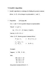
12.Euclid’s Algorithm:
Euclid’s algorithm is a fast method for finding the greatest
common divisor (GCD) of a collection of elements in an Euclidean
domain.
Theorem (Theorem 6.2, page 273)
For a (n, k) RScode,with ν –error and s–erasure in the received
word. Forney syndrome polynomial T(x) is expressed by
T(
x)
≡
S(
x)
τ ( x)
mod
d −1
x
Consider the two polynomials
d −1
x
and T(x) in eq. (6-39). The
m
Euclidean algorithm for polynomials over GF( 2 ) can be used to
develop two finite sequences R i
(x)
and Λ (x)
from the
following two recursive formulas:
Λ
i
( x)
= ( −Qi−1(
x))
Λ
i−1(
x)
+ Λ
i−2(
x)
and R x)
= R ( x)
− Q ( x)
R ( )
i
(
i−2 i−1
i−1
x
i
For
i = 1,
2, L,
2t
, where the initial conditions are
Λ
Λ
( x)
= τ ( x)
R ( x)
= T(
x)
d−1
x
0
0
− 1(
x)
= 0 R−1
( x)
=
Here ( )
Q x i−1 is obtained as the principal part of
R
R
i−2
i−1
( x)
( x)
.

The recursion in eq. (6-40a) and eq. (6-40b) for R i
(x)
and
Λ
i
(x) terminates when deg{ R i
( x)}
≤ ⎣(
d + ν − 3) 2⎦
for the
first time for some value
i = i'
Let
and
A( x)
= R
'(
x)
/ ∆
Λ ( x)
= Λ ( x)
/ ∆
i
i
Also in eq. (6.41) ∆ = Λ i'
(0)
m
is a field element in GF( 2 )which
is chosen so that Λ = 0
1 .
The pair of polynomials A(x) and Λ(x)
in eq. (6.41) constitute
the unique solution of
A ( x)
≡ T(
x)
Λ(
x)
mod
d −1
x
,whereboth
of the inequlaities, deg{ Λ(
x)}
≤ ⎣(
d + ν − 1) 2⎦
and deg{ A(
x)}
≤ ⎣(
d + ν − 3) 2⎦
are satisfied.
Errata-value computation
The locations of the errata can be obtained by finding the roots of
Λ(x)
using the Chien search procedure.
By eq. (6. 34), it is shown readily that the errata values are
−1
A(
X
j
)
Y
j
for j = 1, 2, L,ν
+ s
= −
j
j
b−1
1
( X Λ'(
X ))
−1
where Λ'(
X ) is the derivative with respect to x of Λ (x)
,
j
evaluated at
x .
−1
= X
j

The overall decoding process of RS codes for correcting errors
and erasures, which used the Euclidean algorithm, is summarized
in the following steps:
(1) Compute the syndrome S1 , S2,
L,
S2t
with all of the erasure
positions in the received word being replaced by 0s from eq.
(6. 29), (6. 30) and next calculate λ(x)
from eq. (6. 31) and
let
deg{ λ ( x )} = ν .
(2) Compute the Forney syndrome polynomial from T(x) bythe
use of eq. (6. 37)
(3) To determine Λ(x)
and A(x), where 0 ≤ν
≤ d − 1 , apply the
Euclidean algorithm to
d−1
x and T(x) as given by eq. (6. 39)
The initial values are
Λ
Λ
( x)
= τ ( x)
R ( x)
= T(
x)
d −1
x
0
0
− 1(
x)
= 0 R−1
( x)
=
For ν = d − 1 ,set Λ( x)
= τ ( x)
and A ( x)
= T(
x)
(4) Compute the errata value from eq. (6. 42)

Example 6.10 (page 277)
Consider the (15, 9) RS code, α 15 = 1
The minimum distance of the code is d =7
In this code, s erasures and ν
errors under the condition
s + 2ν ≤ d − 1 can be corrected.
Assuming that the received word is
r
= ( α
10
, α
12
8 5
, α , α , α , α
14
, α
13
9 9
, α , α , 1 , α , α
12
6
, α , α
12
8
, α )
Also assume that the erasure vector is
e*
=
(0 , 0 , 0 , 0 , 0 , 0 ,
And the error vector is
2
0, α ,
0 , 0 , 0 ,
0 , 0 , 0 , 0)
e
= (0 , 0 , 0 , 0 , α
11
,
0 , 0 , 0 , 0 , 0 ,
7
0 , α ,
0 , 0 , 0)
The errata vector is
u
=
(0 , 0 ,
0 , 0 , α
11
, 0 ,
2
0, α ,
0 , 0 ,
7
0 , α ,
0 , 0 , 0)
The syndrome
Si
satisfy
S
i
14
ij
= ∑rjα
j=
0
7 3
= α ( α )
i
2 7
+ α ( α )
i
+ α
11
( α
10
)
i
for
1 ≤ i ≤ 6
This yields
S
S
1
2
= 1
= α
13
S
S
3
4
= α
= α
14
11
S
S
5
6
= α
= 0
Thus
S
13 14 2 11 3 14
( x)
= 1 + α x + α x + α x + αx

The erasure locator polynomial is
7
τ ( x)
= 1 + α x
By eq. (6. 39),
d −1
T(
x)
≡ S(
x)
τ ( x)
mod x ,
one obtains
7
13 14 2
T(
x)
≡ (1 + α x)(1
+ α x + α x
8 5 9 4 3 12
= α x + α x + αx
+ α x
11 3
+ α x + αx
5
+ α x + 1
2
4
)
mod
x
6
Now applying the Euclidean algorithm to
Initial conditions:
d−1
x
and T(x).
R
R
Λ
Λ
−1
0
0
−1
d−1
6
( x)
= x = x
8 5 9
( x)
= T(
x)
= α x + α x
7
( x)
= τ ( x)
= 1 + α x
( x)
= 0
4
+ αx
3
12
+ α x
2
5
+ α x + 1
d = 7 ν = 2
Iterations:
Λ ( x)
= ( −Q
1(
x))
Λ
1(
x)
+ Λ
2(
x)
i
i−
i−
i−
R ( x)
= R
2(
x)
− Q
1(
x)
R
1(
x)
Q
i
i−1
i−
⎡ Ri
( x)
= ⎢
⎣ Ri
−2
−1
( x)
⎤
( x)
⎥
⎦
i−
i−