Chapter 5 BCH Codes

You also want an ePaper? Increase the reach of your titles
YUMPU automatically turns print PDFs into web optimized ePapers that Google loves.
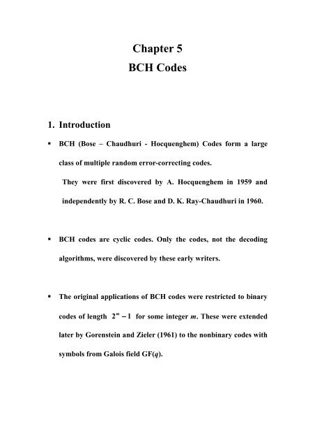
<strong>Chapter</strong> 5<br />
<strong>BCH</strong> <strong>Codes</strong><br />
1. Introduction<br />
<br />
<strong>BCH</strong> (Bose – Chaudhuri - Hocquenghem) <strong>Codes</strong> form a large<br />
class of multiple random error-correcting codes.<br />
They were first discovered by A. Hocquenghem in 1959 and<br />
independently by R. C. Bose and D. K. Ray-Chaudhuri in 1960.<br />
<br />
<strong>BCH</strong> codes are cyclic codes. Only the codes, not the decoding<br />
algorithms, were discovered by these early writers.<br />
<br />
The original applications of <strong>BCH</strong> codes were restricted to binary<br />
m<br />
codes of length 2 − 1<br />
for some integer m. These were extended<br />
later by Gorenstein and Zieler (1961) to the nonbinary codes with<br />
symbols from Galois field GF(q).
The first decoding algorithm for binary <strong>BCH</strong> codes was devised<br />
by Peterson in 1960. Since then, Peterson’s algorithm has been<br />
refined by Berlekamp, Massey, Chien, Forney, and many others.<br />
2. Primitive <strong>BCH</strong> <strong>Codes</strong><br />
For any integer m ≥ 3<br />
and<br />
t < 2 m−1<br />
there exists a primitive<br />
<strong>BCH</strong> code with the following parameters:<br />
m<br />
n = 2 − 1<br />
n − k ≤ mt<br />
dmin ≥ 2t<br />
+ 1<br />
(5- 1)<br />
<br />
This code can correct t or fewer random errors over a span of<br />
m<br />
2 − 1<br />
bit positions.<br />
Thecodeisat-error-correcting <strong>BCH</strong> code.<br />
For example, for m=6, t=3<br />
6<br />
n = 2 − 1 = 63<br />
n − k = 6 × 3 = 18<br />
d = 2×<br />
3 + 1 = 7<br />
min<br />
This is a triple-error-correcting (63, 45) <strong>BCH</strong> code.
3. Generator Polynomial of Binary <strong>BCH</strong> <strong>Codes</strong><br />
m<br />
Let α be a primitive element in GF( 2 ).<br />
For<br />
1 ≤ i ≤ t ,let φ )<br />
( 2i−1 x<br />
be the minimum polynomial of the<br />
field element<br />
2i−1<br />
α .<br />
Thedegreeof φ2i−1(<br />
x)<br />
is m or a factor of m.<br />
<br />
The generator polynomial g(x) ofat-error-correcting primitive<br />
m<br />
<strong>BCH</strong> codes of length 2 − 1<br />
is given by<br />
{ ( x),<br />
φ ( x),<br />
, ( )}<br />
g( x)<br />
= LCM φ1 3<br />
L φ2t−1<br />
x<br />
(5- 2)<br />
<br />
Note that the degree of g(x)ismt or less.<br />
Hence the number of parity-check bits; n-k, of the code is at<br />
most mt.<br />
Example 5.1, 5.2, 5.3, 5.4. (pp. 191-196)<br />
(m =4,m =5)
Note that the generator polynomial of the binary <strong>BCH</strong> code is<br />
originally found to be the least common multiple of the minimum<br />
polynomials<br />
φ , φ<br />
1<br />
φ<br />
2,<br />
L,<br />
2t<br />
i.e. g x)<br />
= LCM{ φ ( x),<br />
φ ( x),<br />
φ ( x),<br />
L,<br />
φ ( x),<br />
φ ( )}<br />
(<br />
1 2 3<br />
2t−1<br />
2t<br />
x<br />
However, generally, every even power of α<br />
m<br />
in GF( 2 )hasthesame<br />
minimal polynomial as some preceding odd power of α<br />
2m<br />
in GF( 2 ).<br />
As a consequence, the generator polynomial of the t-error-correcting<br />
binary <strong>BCH</strong> code can be reduced to<br />
{ ( x),<br />
φ ( x),<br />
, ( )}<br />
g( x)<br />
= LCM φ1 3<br />
L φ2t−1<br />
x .
Example: m =4,t =3<br />
Let α<br />
4<br />
be a primitive element in GF( 2 ) which is constructed<br />
based on the primitive polynomial<br />
p ( x)<br />
= 1 + x + x<br />
4<br />
φ ( x + x + x<br />
1<br />
) = 1<br />
4<br />
corresponding to α<br />
φ<br />
2 3 4<br />
3<br />
( x ) = 1 + x + x + x + x<br />
corresponding to<br />
3<br />
α<br />
φ ( x + x + x<br />
5<br />
) = 1<br />
2<br />
corresponding to<br />
5<br />
α<br />
{ φ ( x),<br />
φ ( x),<br />
φ ( x)<br />
}<br />
g(<br />
x)<br />
= LCM<br />
1 3<br />
= φ1(<br />
x)<br />
φ3<br />
( x)<br />
φ5<br />
( x)<br />
2 4<br />
= 1 + x + x + x + x<br />
5<br />
5<br />
+ x<br />
The code is a (15, 5) cyclic code.<br />
8<br />
+ x<br />
10
4. Properties of Binary <strong>BCH</strong> <strong>Codes</strong><br />
Consider a t-error-correcting <strong>BCH</strong> code of length n = 2 m − 1<br />
with generator polynomial g(x).<br />
<br />
g(x) has as<br />
2 3 2t<br />
α, α , α , L,<br />
α roots, i.e.<br />
i<br />
g( α ) = 0 for 1 ≤ i ≤ 2t<br />
(5-<br />
3)<br />
<br />
Since a code polynomial c(x) is a multiple of g(x), c(x) alsohas<br />
2 2t<br />
i<br />
α, α , L,<br />
α as roots, i.e. c( ) = 0 for 1 ≤ i ≤ 2t<br />
α .<br />
m<br />
A polynomial c(x)ofdegreelessthan 2 − 1<br />
is a code polynomial<br />
ifandonlyifithas<br />
2 2t<br />
α, α , L,<br />
α as roots.
5. Decoding of <strong>BCH</strong> <strong>Codes</strong><br />
Consider a <strong>BCH</strong> code with n = 2 m − 1<br />
and generator polynomial<br />
g(x).<br />
Suppose a code polynomial<br />
n−1<br />
c(<br />
x)<br />
= c0<br />
+ c1x<br />
+ L+<br />
c n −1x<br />
is<br />
transmitted.<br />
Let<br />
n−1<br />
r(<br />
x)<br />
= r0<br />
+ r1<br />
x + L+<br />
r n −1x<br />
be the received polynomial.<br />
<br />
Then r(x)=c(x)+e(x), where e(x) is the error polynomial.<br />
<br />
To check whether r(x) is a code polynomial or not, we simply test<br />
2<br />
2t<br />
whether r(<br />
α)<br />
= r(<br />
α ) = L = r(<br />
α ) = 0 .<br />
If yes, then r(x) is a code polynomial, otherwise r(x) is not a code<br />
polynomial and the presence of errors is detected.<br />
<br />
Decoding procedure<br />
(1) syndrome computation.<br />
(2) determination of the error pattern.<br />
(3) error correction.
6. Syndrome computation<br />
<br />
m<br />
The syndrome consists of 2t components in GF( 2 )<br />
S<br />
= S S L S )<br />
(5-<br />
(<br />
1 2 2t<br />
4)<br />
i<br />
and S = r(<br />
α ) for 1 ≤ i ≤ 2t<br />
.<br />
i<br />
<br />
Computation:<br />
Let φ (x)<br />
i<br />
be the minimum polynomial of<br />
i<br />
α .<br />
Dividing r(x)by φ (x)<br />
,weobtain<br />
r( x)<br />
= a(<br />
x)<br />
φ<br />
i<br />
( x)<br />
+ b(<br />
x)<br />
i<br />
i<br />
Then S = b(<br />
α )<br />
(5- 5)<br />
i<br />
i<br />
S = b(<br />
α ) can be obtained by linear feedback shift-register with<br />
i<br />
connection based on φ (x)<br />
.<br />
i
7. Syndrome and Error Pattern<br />
<br />
Since r(x)=c(x)+e(x)<br />
i<br />
i<br />
i<br />
i<br />
then s = r(<br />
α ) = c(<br />
α ) + e(<br />
α ) = e(<br />
α )<br />
(5-<br />
6)<br />
i<br />
for<br />
1 ≤ i ≤ 2t<br />
.<br />
This gives a relationship between the syndrome and the error<br />
pattern.<br />
Suppose e(x) hasν errors ( ν ≤ t)<br />
at the locations specified by<br />
j j2<br />
x , x , ,<br />
1 L j<br />
x ν<br />
.<br />
i.e.<br />
e = L+<br />
j1<br />
j2<br />
j<br />
( x)<br />
x + x + x ν<br />
(5- 7)<br />
where ≤ j < j < L < j ≤ n 1 .<br />
0<br />
1 2<br />
ν<br />
−<br />
<br />
From equations (5-6) & (5-7), we have the following relation<br />
between syndrome components and error location:<br />
S<br />
S<br />
S<br />
1<br />
2<br />
2t<br />
j1<br />
= e(<br />
α)<br />
= α<br />
j2<br />
+ α<br />
jν<br />
+ L + α<br />
2 j1<br />
2<br />
= e(<br />
α ) = ( α )<br />
j2<br />
2<br />
+ ( α )<br />
jν<br />
2<br />
+ L+<br />
( α )<br />
M<br />
2t<br />
j1<br />
2t<br />
= e(<br />
α ) = ( α )<br />
j2<br />
2t<br />
+ ( α )<br />
jν<br />
+ L + ( α )<br />
2t<br />
(5- 8)
It we can solve the 2t equations, we can determine<br />
j<br />
α<br />
1 j2<br />
jν<br />
, α , L , α .<br />
ju The unknown parameter α = Z<br />
u for u = 1,2,<br />
L,<br />
ν<br />
are called<br />
the “error location number”.<br />
When<br />
1 are found, the powers j u ,<br />
ju<br />
α , ≤ u < ν<br />
u = 1,2,<br />
L,<br />
ν<br />
give us the error locations in e(x). these 2t equation of eq. (5-8)<br />
Are known as power-sum symmetric function.
8. Error-Location Polynomial<br />
(Error-Locator Polynomial)<br />
suppose that ν ≤ t<br />
errors actually occur.<br />
Define error-locator polynomial L(z)as<br />
L(<br />
z)<br />
= (1 + Z z)(1<br />
+ Z z)<br />
L(1<br />
+ Z<br />
=<br />
ν<br />
∏<br />
i=<br />
1<br />
(1 + Z z)<br />
= σ + σ z + σ z<br />
0<br />
1<br />
1<br />
i<br />
2<br />
2<br />
2<br />
+ L+<br />
σ z<br />
ν<br />
ν<br />
ν<br />
z)<br />
(5- 9)<br />
where σ = 0<br />
1 .<br />
<br />
L(z)has<br />
Z L as roots.<br />
−1<br />
−1<br />
−1<br />
1<br />
, Z2<br />
, , Z ν<br />
Note that<br />
Z<br />
u<br />
j<br />
= α u<br />
.<br />
If we can determine L(z) from the syndrome S = S , S , L,<br />
S ) ,<br />
(<br />
1 2 2t<br />
then the roots of L(z) give us the error-location numbers.
9. Relationship between S and L(z)<br />
<br />
From eq. (5-9), we find the following relationship between the<br />
coefficients of L(z) and the error-locator numbers:<br />
σ<br />
σ<br />
1<br />
σ<br />
σ<br />
2<br />
ν<br />
=<br />
= Z<br />
= Z<br />
M<br />
= Z<br />
0<br />
1<br />
1<br />
1<br />
1<br />
+ Z2<br />
+ L+<br />
Zν<br />
Z + Z Z + L+<br />
Z<br />
Z<br />
2<br />
2<br />
2<br />
LZ<br />
ν<br />
3<br />
Z<br />
ν − 1 ν<br />
(5- 10)<br />
eq. (5-10) is called “elementary symmetric functions”.<br />
<br />
From eq. (5-8) and eq. (5-10), we have the following relationship<br />
between the syndrome and the coefficients of L(z):<br />
S<br />
ν<br />
+ σ S<br />
1<br />
ν −1<br />
+ σ S<br />
2<br />
S<br />
3<br />
ν −2<br />
S<br />
+ σ S<br />
1<br />
2<br />
2<br />
+ L+<br />
σ<br />
S1<br />
+ σ<br />
1<br />
+ σ<br />
1S1<br />
+ 2σ<br />
2<br />
+ σ S + 3σ<br />
2<br />
ν −1<br />
S<br />
1<br />
1<br />
+<br />
νσ<br />
3<br />
ν<br />
= 0<br />
= 0<br />
= 0<br />
M<br />
= 0<br />
(5- 11)<br />
Here for binary case<br />
iσ = σ<br />
i<br />
i<br />
when i is odd,<br />
and iσ = 0<br />
i<br />
otherwise.<br />
<br />
The equations of (5-11) are called the Newton’s identities.
If we can determine σ , σ , 1 2<br />
L,<br />
σ<br />
ν from the Newton’s identities,<br />
then we can determine the error-location numbers<br />
Z , Z , 2<br />
, Z<br />
1<br />
L<br />
ν ,<br />
by finding the roots of L(z).<br />
<br />
Note that the Newton’s identities in (5-11) can be expressed also in<br />
the following single-equation form:<br />
S<br />
i<br />
+<br />
1 i−1<br />
2 i−2<br />
i−1<br />
1 i<br />
L<br />
σ S + σ S + L + σ S + iσ<br />
= 0 for i = 1,2, , ν<br />
(5- 12)
10.Peterson’s Direct-Solution (W. W. Peterson, 1960)<br />
Considerthecasefor i > ν<br />
First multiply L(z) in eq. (5-9) By<br />
i<br />
z − , we have<br />
z<br />
−i<br />
L<br />
−i<br />
1−i<br />
2−i<br />
ν −1−i<br />
ν −i<br />
( z)<br />
= z + σ<br />
1z<br />
+ σ<br />
2z<br />
+ L + σ ν −1z<br />
+ σ<br />
ν<br />
z (5- 13)<br />
<br />
Next substituting the roots of L(z) (i.e.<br />
Z L ) into eq.<br />
−1<br />
−1<br />
−1<br />
1<br />
, Z2<br />
, , Z ν<br />
(5-13) produces the following set of equations:<br />
Z<br />
Z<br />
Z<br />
i<br />
1<br />
i<br />
2<br />
i<br />
ν<br />
+ σ<br />
1Z<br />
+ σ Z<br />
1<br />
+ σ Z<br />
1<br />
i−1<br />
1<br />
i−1<br />
2<br />
i−1<br />
ν<br />
+ σ<br />
2<br />
Z<br />
+ σ Z<br />
2<br />
+ σ Z<br />
2<br />
i−2<br />
1<br />
i−2<br />
2<br />
i−2<br />
ν<br />
+ L + σ<br />
+ L + σ<br />
+ L + σ<br />
ν −1<br />
ν −1<br />
ν −1<br />
Z<br />
Z<br />
Z<br />
i−ν<br />
+ 1<br />
1<br />
i−ν<br />
+ 1<br />
2<br />
i−ν<br />
+ 1<br />
ν<br />
+ σ<br />
ν<br />
Z<br />
+ σ Z<br />
ν<br />
+ σ Z<br />
ν<br />
i−ν<br />
1<br />
i−ν<br />
2<br />
i−ν<br />
ν<br />
= 0<br />
= 0<br />
M<br />
= 0<br />
(5- 14)<br />
Adding these ν<br />
equation term by term yield<br />
( Z<br />
i<br />
1<br />
+ Z<br />
i<br />
2<br />
+ L+<br />
Z<br />
i<br />
ν<br />
i−1<br />
i−1<br />
) + σ<br />
1(<br />
Z1<br />
+ Z<br />
2<br />
+ L+<br />
Z<br />
i−ν<br />
i−ν<br />
+ σ ( Z , Z , L,<br />
Z<br />
ν<br />
1<br />
2<br />
i−1<br />
ν<br />
i−ν<br />
ν<br />
) + L<br />
) = 0<br />
(5- 15)<br />
<br />
Now express eq. (5-15) in terms of syndrome components, then<br />
S<br />
i<br />
+<br />
−<br />
σ<br />
1Si−1<br />
+ L + σ<br />
ν −1Si−ν<br />
+ 1<br />
+ σ<br />
ν<br />
Si<br />
ν<br />
= 0 for i > ν (5- 16)<br />
In particular, for i =ν + 1 ,weobtain<br />
S<br />
ν + 1<br />
+<br />
1 ν<br />
ν −1<br />
2 ν<br />
S1<br />
=<br />
σ S + L + σ S + σ 0<br />
(5- 17)<br />
Thus, the Newton’s identities can be extended to the unknown<br />
syndrome<br />
S for i > ν .<br />
i
From eq. (5-16) & eq. (5-17), we can see that the σ<br />
j<br />
for<br />
0 ≤ j ≤ν are closely related to the syndrome components S<br />
i ,<br />
1 ≤ i ≤ν<br />
+ 1 .<br />
Thus, σ<br />
j<br />
can be determined by solving the set of syndrome<br />
equations eq. (5-16) & eq. (5-17). Then the error-locations for can<br />
be found by solving<br />
ju α = Z<br />
u for ≤ u ≤ν<br />
1 the root of L(z). This<br />
L(z) produces an error-pattern e(x) with the minimum number of<br />
errors. Hence if<br />
ν ≤<br />
t<br />
errors occur, L(z) will give the actual error<br />
pattern e(x).<br />
<br />
Finally, the error-correcting procedure for the binary <strong>BCH</strong> codes<br />
can be outlined as follows:<br />
(1) Compute the syndrome components S<br />
j ,<br />
1 ≤ j ≤ 2t<br />
,fromthe<br />
received polynomial r(x). [eq. (5-5)]<br />
(2) Set each σ = 0 for ν + 1 ≤ j ≤ t<br />
j<br />
and solve the first ν equations of eq. (5-11) for the σ<br />
j ,<br />
1 ≤ j ≤ν in terms of S<br />
j .<br />
(3) Determine the error-locator polynomial L(z) fromthese σ<br />
j
in terms of syndrome component<br />
S for 0 ≤ j ≤ 2t<br />
.<br />
j<br />
(4) Find the error-location numbers Z , Z , 1 2<br />
L,<br />
Zν<br />
by solving<br />
for the roots of L(z). Use these roots to correct the errors in<br />
r(x).
11.Direct Solutions of Some Simple Cases.<br />
(1) Single-error correction:<br />
σ<br />
1<br />
= S1<br />
L(<br />
z)<br />
= 1 + S1z<br />
S1<br />
≠ 0<br />
3<br />
S3<br />
= S1<br />
(2) Double-error correction:<br />
σ<br />
σ<br />
1<br />
2<br />
= S<br />
1<br />
= S<br />
−1<br />
1<br />
( S<br />
3<br />
+ S<br />
3<br />
1<br />
)<br />
3<br />
S1<br />
≠ 0, S3<br />
≠ S1<br />
3<br />
⎡ S1<br />
+ S<br />
L(<br />
z)<br />
= 1 + S1z<br />
+ ⎢<br />
⎣ S<br />
1<br />
3<br />
⎤<br />
⎥z<br />
⎦<br />
2<br />
(3) Triple-error correction:<br />
σ<br />
σ<br />
σ<br />
1<br />
2<br />
3<br />
= S<br />
S<br />
=<br />
= ( S<br />
1<br />
2<br />
1<br />
S3<br />
3<br />
S1<br />
3<br />
1<br />
+ S<br />
3<br />
5<br />
+ S3<br />
+ S ) + S σ<br />
1<br />
2<br />
S<br />
S<br />
1<br />
3<br />
≠ 0<br />
≠ S<br />
3<br />
1<br />
4<br />
Example: m =4,t = 3 <strong>BCH</strong> code over GF( 2 ).<br />
The primitive polynomial for m =4is<br />
φ( x ) = 1+<br />
x + x<br />
4<br />
The minimum polynomials of α ,<br />
3<br />
α<br />
and<br />
5<br />
α<br />
are<br />
φ1(<br />
x)<br />
= 1 + x + x<br />
φ3(<br />
x)<br />
= 1 + x + x<br />
φ ( x)<br />
= 1 + x + x<br />
5<br />
4<br />
2<br />
2<br />
+ x<br />
3<br />
+ x<br />
4<br />
n = 2 4 − 1 =<br />
15<br />
g(<br />
x)<br />
= LCM{<br />
φ1(<br />
x),<br />
φ<br />
3(<br />
x),<br />
φ5<br />
( x)}<br />
= φ1φ<br />
3φ5<br />
2 4 5 8<br />
= 1 + x + x + x + x + x + x<br />
10
The code is a (15, 5) cyclic code.<br />
The generator polynomial g(x) has<br />
α<br />
2 3 4 5 6<br />
, α , α , α , α , α<br />
as<br />
roots. The roots α ,<br />
2<br />
α<br />
and<br />
4<br />
α<br />
have the same polynomial<br />
φ ( x + x + x<br />
1<br />
) = φ2(<br />
x)<br />
= φ4<br />
( x)<br />
= 1<br />
4<br />
The root<br />
3<br />
α<br />
and<br />
6<br />
α<br />
have the same minimum polynomial<br />
φ<br />
2 3 4<br />
3( x ) = φ6<br />
( x)<br />
= 1 + x + x + x + x<br />
The minimum polynomial of<br />
5<br />
α<br />
is<br />
φ ( x + x + x<br />
5<br />
) = 1<br />
2<br />
Suppose all-zero code word c = ( 0 0 0L0)<br />
is transmitted<br />
and<br />
r ( x)<br />
+ x<br />
2 5 12<br />
= x + x is received.<br />
Dividing r(x)by φ ( ) , φ ( ) and φ ( ) , respectively,<br />
1 x<br />
we obtain the remainders:<br />
b1<br />
( x)<br />
= 1<br />
b3<br />
( x)<br />
= 1 + x + x<br />
2<br />
b ( x)<br />
= x<br />
5<br />
3<br />
3 x<br />
5 x<br />
The syndrome components are<br />
s<br />
s<br />
s<br />
s<br />
s<br />
s<br />
1<br />
2<br />
4<br />
3<br />
6<br />
5<br />
= b1<br />
( α)<br />
= 1<br />
2<br />
= b1<br />
( α ) = 1<br />
4<br />
= b1<br />
( α ) = 1<br />
3<br />
6 9 10<br />
= b3<br />
( α ) = 1 + α + α = α<br />
6<br />
12 18 5<br />
= b3<br />
( α ) = 1 + α + α = α<br />
5 10<br />
= b ( α ) = α<br />
3<br />
10 10 5<br />
Hence S = (1 , 1 , α , 1 , α , α ) .
Example: (p. 209) consider t =2,m = 5, (32, 21) <strong>BCH</strong> code<br />
The primitive polynomial for m =5is<br />
φ<br />
2 5<br />
( x ) = 1 + x + x<br />
α<br />
2 4 8<br />
, α , α , α<br />
and<br />
16<br />
α<br />
have the same minimum polynomial<br />
α<br />
3 6 12 24<br />
, α , α , α<br />
and<br />
17<br />
α<br />
have the same minimum polynomial<br />
φ<br />
2 3 4 5<br />
3( x ) = 1 + x + x + x + x<br />
α<br />
5 10 20 9<br />
, α , α , α<br />
and<br />
8<br />
α<br />
have the same minimum polynomial<br />
φ<br />
2 4 5<br />
5( x ) = 1 + x + x + x + x<br />
α<br />
7 14 28 25<br />
, α , α , α<br />
and<br />
19<br />
α<br />
have the same minimum polynomial<br />
φ<br />
2 3 5<br />
7<br />
( x ) = 1 + x + x + x + x<br />
α<br />
11 22 13 26<br />
, α , α , α<br />
and<br />
21<br />
α<br />
have the same minimum polynomial<br />
φ<br />
3 4 5<br />
11( x ) = 1 + x + x + x + x<br />
The generator polynomial of (32, 21) code is<br />
g +<br />
3 5 6 8 9 10<br />
( x)<br />
= φ1(<br />
x)<br />
φ3(<br />
x)<br />
= 1 + x + x + x + x + x x<br />
The roots of the generator polynomial include<br />
α<br />
2 3<br />
, α , α<br />
and<br />
4<br />
α<br />
Since<br />
r +<br />
2 7 8 11 12<br />
( x)<br />
= x + x + x + x x
We obtain<br />
S<br />
S<br />
S<br />
S<br />
1<br />
2<br />
3<br />
4<br />
7<br />
= r(<br />
α)<br />
= α<br />
2<br />
= r(<br />
α ) = α<br />
3 8<br />
= r(<br />
α ) = α<br />
4<br />
= r(<br />
α ) = α<br />
14<br />
28<br />
Note here that<br />
S =<br />
2 4<br />
4<br />
= ( S2<br />
) ( S1<br />
)<br />
Then the error-locator polynomial is obtained by the equation<br />
7<br />
σ<br />
1<br />
= α<br />
8 7 3<br />
α + ( α ) 15<br />
σ<br />
2<br />
= = α<br />
7<br />
α<br />
7 15<br />
∴L(<br />
z)<br />
= 1 + α z + α z<br />
5 31−26<br />
∴ Z1<br />
= α = α<br />
10 31−21<br />
Z = α = α<br />
2<br />
2<br />
5<br />
10<br />
= (1 + α z)(1<br />
+ α z)<br />
Thereby indicating errors at 26 th and 21 st coordinates of r<br />
∴c +<br />
2 5 7 8 10 11 12<br />
( x)<br />
= x + x + x + x + x + x x<br />
(Note<br />
Zi<br />
r<br />
= α i<br />
)
12.Computation of Error-Location Numbers<br />
– Chien Search. (R.T. Chien, 1964)<br />
A Chien-search circuit is shown in Fig. 5.2.<br />
L ( z ) = σ<br />
where σ 0<br />
= 1<br />
ν<br />
ν<br />
+ σ z + σ z 2<br />
+ L + σ z<br />
0 1 2<br />
ν<br />
= ∏(1<br />
+ Z z i<br />
)<br />
i=<br />
1<br />
m<br />
The roots of L(z) inGF( 2 ) can be determined by substituting<br />
m<br />
the elements of GF( 2 )inL(z).<br />
i<br />
If L( α ) = 0 ,then<br />
i<br />
α<br />
is the root of L(z) and<br />
α<br />
− i<br />
= α<br />
n−i<br />
is an<br />
error-location number.<br />
To decode the first received digit r<br />
n−1<br />
, we check whether α is a<br />
root of L(z). If L ( α)<br />
= 0 , then rn−<br />
1<br />
is erroneous and must be<br />
corrected.<br />
If L ( α)<br />
≠ 0 ,then rn−<br />
1<br />
is error-free.<br />
i<br />
i<br />
To decode rn<br />
− i ,wetestwhether L( α ) = 0 .if L( α ) = 0 , n i<br />
r −<br />
is<br />
erroneous and must be corrected, otherwise<br />
rn<br />
− i<br />
is error free.
= ( r ,r , L,<br />
1)<br />
0 1<br />
rn-<br />
c'<br />
c'<br />
<br />
<br />
<br />
c'<br />
e i<br />
e<br />
i<br />
⎧ 1, if Di<br />
= 1<br />
= ⎨<br />
⎩0,<br />
otherwise<br />
<br />
D<br />
i<br />
t<br />
ij<br />
= ∑σ<br />
jα<br />
j=<br />
1<br />
i<br />
= L(α<br />
) − 1<br />
<br />
∑<br />
σ 1<br />
σ<br />
2<br />
L<br />
σ<br />
t<br />
2<br />
α α<br />
t<br />
α<br />
Figure 5.2 Chien search and error-correction for binary code.
13.Peterson-Gorenstein-Zierler Decoding Algorithm<br />
From equation (5-16) [Chen / Reed eq. (5-38)]<br />
σ<br />
ν<br />
S<br />
j−ν<br />
+ σ<br />
ν −<br />
S<br />
j−ν<br />
+<br />
+ + σ S<br />
j−<br />
= −S<br />
j<br />
for j > ν<br />
1 1<br />
L<br />
1<br />
1<br />
Assuming that<br />
ν =<br />
t ,then<br />
σ S σ S + L + S = −S<br />
for j t (5- 18)<br />
t j−t<br />
+<br />
t−1 j−t+<br />
1<br />
σ<br />
1 j−1<br />
j<br />
><br />
e.g. j = t + 1, we have<br />
σ S<br />
t<br />
1<br />
+ σ<br />
t−1S2<br />
+ L+<br />
σ<br />
1St<br />
= −St+<br />
1<br />
The following matrix equation is obtained for the symmetric<br />
function<br />
σ<br />
j<br />
as follows:<br />
S'<br />
Λ =<br />
⎡S<br />
⎢<br />
S<br />
⎢<br />
⎢ M<br />
⎢<br />
⎣S<br />
1<br />
2<br />
t<br />
S<br />
S<br />
S<br />
M<br />
2<br />
3<br />
t+<br />
1<br />
L<br />
L<br />
S<br />
S<br />
t−1<br />
S<br />
M<br />
t<br />
2t−2<br />
S<br />
S<br />
S<br />
t<br />
t+<br />
1<br />
M<br />
2t−1<br />
⎤⎡<br />
σ<br />
t<br />
⎥⎢<br />
σ<br />
⎥⎢<br />
t−<br />
⎥⎢<br />
M<br />
⎥⎢<br />
⎦⎣<br />
σ<br />
1<br />
1<br />
⎤<br />
⎥<br />
⎥<br />
⎥<br />
⎥<br />
⎦<br />
=<br />
⎡−<br />
⎢<br />
−<br />
⎢<br />
⎢<br />
⎢<br />
⎣ −<br />
S<br />
S<br />
M<br />
S<br />
t+<br />
1<br />
t+<br />
2<br />
2t<br />
⎤<br />
⎥<br />
⎥<br />
⎥<br />
⎥<br />
⎦<br />
(5- 19)<br />
It can be shown that S'<br />
is nonsingular if the received word<br />
contains exactly t errors. It also can be shown that<br />
S'<br />
is singular<br />
if fewer than t errors occur. If<br />
S'<br />
is singular, then the rightmost<br />
column and bottom rows can be removed and the determinant of<br />
the resulting matrix computed.
This process is repeated until one reaches a non-singular matrix.<br />
The coefficients of the error-locator polynomial are then founded<br />
by the use of standard algebraic technique.<br />
Once the ν error locations are known, hen we can use the<br />
relation between syndrome components and error locations.<br />
[eq. (5-8)]<br />
The syndrome components can be computed by<br />
S<br />
j<br />
j<br />
= e(<br />
α ) =<br />
n−1<br />
∑<br />
k=<br />
0<br />
e<br />
k<br />
j<br />
⋅ ( α )<br />
k<br />
=<br />
ν<br />
∑<br />
l=<br />
1<br />
e<br />
i<br />
l<br />
⋅ Z<br />
j<br />
l<br />
where<br />
e(<br />
x)<br />
= e<br />
0<br />
+ e<br />
1<br />
x + e<br />
2<br />
x<br />
2<br />
+ L+<br />
e<br />
n<br />
−<br />
∑ − 1<br />
n 1<br />
n− 1<br />
x =<br />
k=<br />
0<br />
e<br />
k<br />
x<br />
k<br />
Thus we have<br />
S<br />
S<br />
S<br />
1<br />
2<br />
2t<br />
= e<br />
i<br />
= e<br />
M<br />
= e<br />
i<br />
i<br />
1<br />
1<br />
1<br />
Z<br />
Z<br />
Z<br />
1<br />
2<br />
1<br />
2t<br />
1<br />
+ e<br />
i<br />
+ e<br />
2<br />
i<br />
2<br />
+ e<br />
i<br />
Z<br />
2<br />
Z<br />
2<br />
2<br />
2<br />
Z<br />
+ L+<br />
e<br />
2t<br />
2<br />
+ L + e<br />
+ L+<br />
e<br />
i<br />
ν<br />
i<br />
ν<br />
Z<br />
i<br />
ν<br />
2<br />
ν<br />
Z<br />
ν<br />
Z<br />
2t<br />
ν
The system equations can be reduced to the following matrix<br />
form:<br />
D ⋅ e<br />
⎡ Z1<br />
⎢ 2<br />
Z<br />
= ⎢<br />
1<br />
⎢ M<br />
⎢<br />
⎣Z1<br />
ν<br />
Z<br />
Z<br />
M<br />
Z<br />
2<br />
2<br />
2<br />
ν<br />
2<br />
L<br />
L<br />
L<br />
Z<br />
Z<br />
Z<br />
ν<br />
2<br />
ν<br />
M<br />
ν<br />
ν<br />
⎤⎡ei<br />
⎥⎢<br />
e<br />
⎥⎢<br />
i<br />
⎥⎢<br />
M<br />
⎥⎢<br />
⎦⎣<br />
ei<br />
1<br />
2<br />
ν<br />
⎤<br />
⎥<br />
⎥ =<br />
⎥<br />
⎥<br />
⎦<br />
⎡S<br />
⎢<br />
S<br />
⎢<br />
⎢ M<br />
⎢<br />
⎣S<br />
1<br />
2<br />
ν<br />
⎤<br />
⎥<br />
⎥<br />
⎥<br />
⎥<br />
⎦<br />
(5- 20)<br />
Decoding is completed by solving for the { e il<br />
}<br />
This is a general case of nonbinary <strong>BCH</strong> codes.<br />
Example (5.9)<br />
Consider a nonbinary <strong>BCH</strong> code (7, 3) of length 7 (symbols) this<br />
code is constructed over GF(8) with generator polynomial<br />
2<br />
3<br />
4<br />
g(<br />
x)<br />
= ( x − α)(<br />
x − α )( x − α )( x − α )<br />
4 3 3 2 3<br />
= x + α x + x + α<br />
Let the received polynomial be<br />
r<br />
2 6 2 4 3 5 2<br />
( x)<br />
= α x + α x + x + α x<br />
Then the syndrome components are<br />
S<br />
3<br />
= α , S = S = S = α<br />
6<br />
3<br />
4<br />
1 2<br />
α ,<br />
3<br />
α ,<br />
4
Eq. (5-19) gives<br />
S' Λ =<br />
6<br />
⎡α<br />
⎢ 3<br />
⎣α<br />
3<br />
α ⎤⎡σ<br />
2 ⎤<br />
4 ⎥⎢<br />
α σ<br />
⎥<br />
⎦⎣<br />
1 ⎦<br />
=<br />
4<br />
⎡α<br />
⎤<br />
⎢ 3 ⎥<br />
⎣α<br />
⎦<br />
⇒ σ<br />
1<br />
2<br />
= α ,<br />
σ<br />
2<br />
= α<br />
2 2<br />
Thus L(<br />
x)<br />
= αx<br />
+ α x + 1<br />
The error locations are founded to be<br />
Z<br />
1<br />
3<br />
= α<br />
= α<br />
7−4<br />
,<br />
Z<br />
2<br />
5<br />
= α<br />
= α<br />
7−2<br />
⇒ e(<br />
x)<br />
= e<br />
3<br />
x<br />
3<br />
+ e<br />
5<br />
x<br />
5<br />
Eq. (5-20) gives<br />
D<br />
3<br />
⎡α<br />
= ⎢ 6<br />
⎣α<br />
5<br />
α ⎤⎡e<br />
3 ⎥⎢<br />
α ⎦⎣e<br />
6<br />
⎤ ⎡α<br />
⎤<br />
⎥ = ⎢ ⎥<br />
⎦ ⎣α<br />
⎦<br />
3<br />
⋅ e<br />
3<br />
5<br />
The error magnitudes are found to be<br />
e<br />
3<br />
= α,<br />
e<br />
5<br />
5<br />
= α<br />
⇒ e(<br />
x)<br />
= αx<br />
3<br />
5<br />
+ α x<br />
5<br />
Finally<br />
c<br />
2 6 5 5 2 4 3 3 5 2<br />
( x)<br />
= e(<br />
x)<br />
+ r(<br />
x)<br />
= α x + α x + α x + α x + α x<br />
Note that m = 3, the primitive polynomial is<br />
p ( x)<br />
= 1 + x + x<br />
3
14.<strong>BCH</strong> <strong>Codes</strong> as Industry Standards<br />
(a) (511, 493) <strong>BCH</strong> code in ITU-T. Rec. H.261 “video codec for<br />
audiovisual service at kbit/s” a video coding a standard used for<br />
video conferencing and video phone.<br />
n = 511<br />
k = 493<br />
m = 9<br />
n − k = 18<br />
t = 2<br />
(b) (40, 32) <strong>BCH</strong> code in ATM (Asynchronous Transfer Mode) pp.<br />
223-227.<br />
This is shortened cyclic code that can correct 1-bit error and<br />
detect 2-bit errors.