A Multiresolution Formulation of Wavelet Systems
A Multiresolution Formulation of Wavelet Systems
A Multiresolution Formulation of Wavelet Systems

You also want an ePaper? Increase the reach of your titles
YUMPU automatically turns print PDFs into web optimized ePapers that Google loves.
A <strong>Multiresolution</strong> <strong>Formulation</strong> <strong>of</strong> <strong>Wavelet</strong> <strong>Systems</strong><br />
Discrete <strong>Wavelet</strong> transforms<br />
Prerequisites<br />
<br />
<br />
<br />
<br />
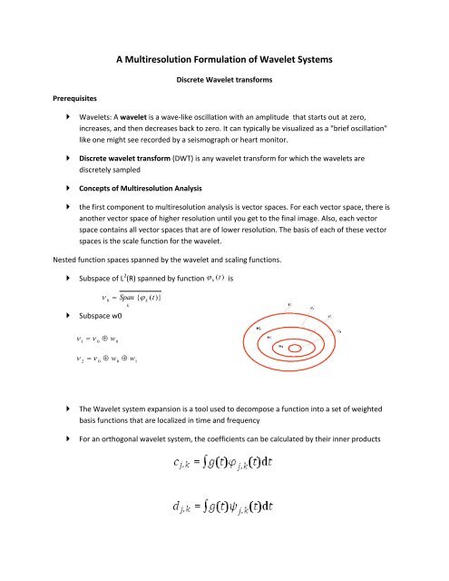
<strong>Wavelet</strong>s: A wavelet is a wave-like oscillation with an amplitude that starts out at zero,<br />
increases, and then decreases back to zero. It can typically be visualized as a "brief oscillation"<br />
like one might see recorded by a seismograph or heart monitor.<br />
Discrete wavelet transform (DWT) is any wavelet transform for which the wavelets are<br />
discretely sampled<br />
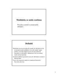
Concepts <strong>of</strong> <strong>Multiresolution</strong> Analysis<br />
the first component to multiresolution analysis is vector spaces. For each vector space, there is<br />
another vector space <strong>of</strong> higher resolution until you get to the final image. Also, each vector<br />
space contains all vector spaces that are <strong>of</strong> lower resolution. The basis <strong>of</strong> each <strong>of</strong> these vector<br />
spaces is the scale function for the wavelet.<br />
Nested function spaces spanned by the wavelet and scaling functions.<br />
Subspace <strong>of</strong> L 2 (R) spanned by function k<br />
(t) is<br />
<br />
Span { ( t)}<br />
0 k<br />
Subspace w0<br />
k<br />
<br />
1<br />
0<br />
w<br />
0<br />
<br />
2<br />
<br />
0<br />
w<br />
0<br />
w<br />
1<br />
<br />
<br />
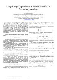
The <strong>Wavelet</strong> system expansion is a tool used to decompose a function into a set <strong>of</strong> weighted<br />
basis functions that are localized in time and frequency<br />
For an orthogonal wavelet system, the coefficients can be calculated by their inner products
Display <strong>of</strong> the Discrete <strong>Wavelet</strong> Transform and the <strong>Wavelet</strong> Expansion<br />
<br />
<br />
Samples <strong>of</strong> the signal – for a high starting scale j 0 samples <strong>of</strong> the signal are the DWT at that<br />
scale.<br />
A 3D plot <strong>of</strong> the expansion coefficients <strong>of</strong> the DWT values c(k) and d j (k)<br />
Components <strong>of</strong> the signal are generated using time functions at each scale:<br />
f ( t ) f<br />
where<br />
f<br />
j0<br />
<br />
<br />
j0<br />
<br />
<br />
c ( k ) ( t k )<br />
j<br />
f<br />
j<br />
( t )<br />
and<br />
f<br />
j<br />
( t ) <br />
<br />
k<br />
d<br />
j<br />
( k )2<br />
j / 2<br />
(2<br />
jt k<br />
)
By generating time functions f k (t) at each translation the time localization <strong>of</strong> the wavelet<br />
expansion is obtain<br />
<br />
f ( t)<br />
c(<br />
k ) ( t k ) d ( k )2 (2 t k )<br />
k<br />
j<br />
j<br />
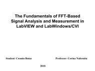
Tilling time frequency plane: we use the term time frequency tile <strong>of</strong> a particular basic function to<br />
designate the region in the plane which contains most <strong>of</strong> the function`s energy<br />
j / 2<br />
j<br />
Generalized tiling which adapts in time as well as in frequency<br />
<br />
The tiling shows the sampling in time and frequency<br />
Examples <strong>of</strong> wavelet expansions<br />
Objective: show the way a wavelet expansion decomposes a signal and what the components look like<br />
at different scale<br />
<br />
<br />
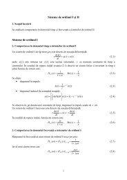
Projection <strong>of</strong> the Houston Skyline Signal onto ν spaceA characteristic <strong>of</strong> Daubechies systems is<br />
that low order polynomials are completely contained in the scaling function space.<br />
DWT used for edge detection
Discrete <strong>Wavelet</strong> Transform <strong>of</strong> a Doppler signal<br />
<br />
Illustrates coefficients <strong>of</strong> the DWT directly as a function <strong>of</strong> j and k
Scaling functions approximations and the wavelet decomposition <strong>of</strong> the chirp signal<br />
Daubechies<br />
Daubechies wavelets<br />
<br />
<br />
the Daubechies wavelets are a family <strong>of</strong> orthogonal wavelets defining a DWT and characterized<br />
by a maximal number <strong>of</strong> vanishing moments for some given support. With each wavelet type <strong>of</strong><br />
this class, there is a scaling function (also called father wavelet) which generates an orthogonal<br />
multiresolution analysis.<br />
Ingrid Daubechies