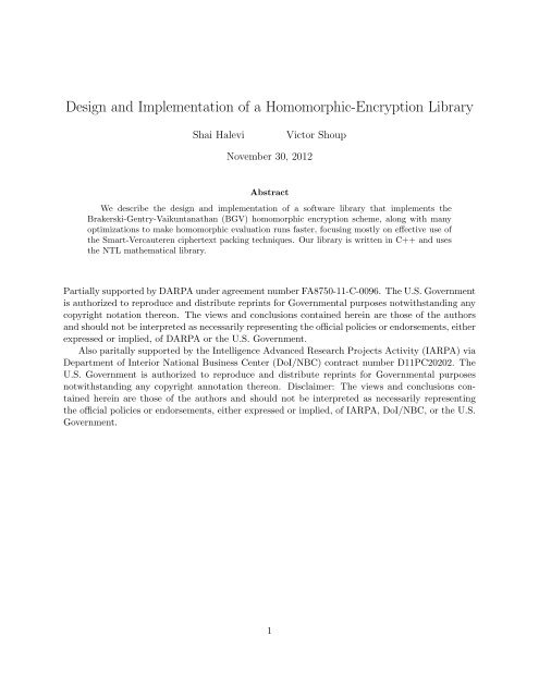
Design and Implementation of a Homomorphic ... - Researcher

Design and Implementation of a Homomorphic-Encryption Library
Shai Halevi
Victor Shoup
November 30, 2012
Abstract
We describe the design and implementation of a software library that implements the
Brakerski-Gentry-Vaikuntanathan (BGV) homomorphic encryption scheme, along with many
optimizations to make homomorphic evaluation runs faster, focusing mostly on effective use of
the Smart-Vercauteren ciphertext packing techniques. Our library is written in C++ and uses
the NTL mathematical library.
Partially supported by DARPA under agreement number FA8750-11-C-0096. The U.S. Government
is authorized to reproduce and distribute reprints for Governmental purposes notwithstanding any
copyright notation thereon. The views and conclusions contained herein are those of the authors
and should not be interpreted as necessarily representing the official policies or endorsements, either
expressed or implied, of DARPA or the U.S. Government.
Also paritally supported by the Intelligence Advanced Research Projects Activity (IARPA) via
Department of Interior National Business Center (DoI/NBC) contract number D11PC20202. The
U.S. Government is authorized to reproduce and distribute reprints for Governmental purposes
notwithstanding any copyright annotation thereon. Disclaimer: The views and conclusions contained
herein are those of the authors and should not be interpreted as necessarily representing
the official policies or endorsements, either expressed or implied, of IARPA, DoI/NBC, or the U.S.
Government.
1

Contents
1 The BGV Homomorphic Encryption Scheme 1
1.1 Plaintext Slots . . . . . . . . . . . . . . . . . . . . . . . . . . . . . . . . . . . . . . . 2
1.2 Our Modulus Chain and Double-CRT Representation . . . . . . . . . . . . . . . . . 2
1.3 Modules in our Library . . . . . . . . . . . . . . . . . . . . . . . . . . . . . . . . . . 3
2 The Math Layers 3
2.1 The timing module . . . . . . . . . . . . . . . . . . . . . . . . . . . . . . . . . . . . 3
2.2 NumbTh: Miscellaneous Utilities . . . . . . . . . . . . . . . . . . . . . . . . . . . . . 3
2.3 bluestein and Cmodulus: Polynomials in FFT Representation . . . . . . . . . . . . . . 4
2.4 PAlgebra: The Structure of Z ∗ m and Z ∗ m/ 〈2〉 . . . . . . . . . . . . . . . . . . . . . . . 5
2.5 PAlgebraModTwo/PAlgebraMod2r: Plaintext Slots . . . . . . . . . . . . . . . . . . . . 6
2.6 IndexSet and IndexMap: Sets and Indexes . . . . . . . . . . . . . . . . . . . . . . . . 8
2.6.1 The IndexSet class . . . . . . . . . . . . . . . . . . . . . . . . . . . . . . . . . 8
2.6.2 The IndexMap class . . . . . . . . . . . . . . . . . . . . . . . . . . . . . . . . . 9
2.7 FHEcontext: Keeping the parameters . . . . . . . . . . . . . . . . . . . . . . . . . . . 9
2.8 DoubleCRT: Efficient Polynomial Arithmetic . . . . . . . . . . . . . . . . . . . . . . . 10
3 The Crypto Layer 13
3.1 The Ctxt module: Ciphertexts and homomorphic operations . . . . . . . . . . . . . . 13
3.1.1 The SKHandle class . . . . . . . . . . . . . . . . . . . . . . . . . . . . . . . . 14
3.1.2 The CtxtPart class . . . . . . . . . . . . . . . . . . . . . . . . . . . . . . . . . 15
3.1.3 The Ctxt class . . . . . . . . . . . . . . . . . . . . . . . . . . . . . . . . . . . 15
3.1.4 Noise estimate . . . . . . . . . . . . . . . . . . . . . . . . . . . . . . . . . . . 16
3.1.5 Modulus-switching operations . . . . . . . . . . . . . . . . . . . . . . . . . . . 18
3.1.6 Key-switching/re-linearization . . . . . . . . . . . . . . . . . . . . . . . . . . 19
3.1.7 Native arithmetic operations . . . . . . . . . . . . . . . . . . . . . . . . . . . 21
3.1.8 More Ctxt methods . . . . . . . . . . . . . . . . . . . . . . . . . . . . . . . . 23
3.2 The FHE module: Keys and key-switching matrices . . . . . . . . . . . . . . . . . . . 24
3.2.1 The KeySwitch class . . . . . . . . . . . . . . . . . . . . . . . . . . . . . . . . 24
3.2.2 The FHEPubKey class . . . . . . . . . . . . . . . . . . . . . . . . . . . . . . . 25
3.2.3 The FHESecKey class . . . . . . . . . . . . . . . . . . . . . . . . . . . . . . . 27
3.3 The KeySwitching module: What matrices to generate . . . . . . . . . . . . . . . . . 28
4 The Data-Movement Layer 29
4.1 The classes EncryptedArray and EncryptedArrayMod2r . . . . . . . . . . . . . . . . . . 29
5 Using the Library 33
5.1 Homomorphic Operations over GF (2 8 ) . . . . . . . . . . . . . . . . . . . . . . . . . . 34
5.2 Homomorphic Operations over Z 2 5 . . . . . . . . . . . . . . . . . . . . . . . . . . . . 35
A Proof of noise-estimate 37

Organization of This Report
We begin in Section 1 with a brief high-level overview of the BGV cryptosystem and some important
features of the variant that we implemented and our choice of representation, as well as an overview
of the structure of our library. Then in Sections 2, 3,4 we give a bottom-up detailed description of
all the modules in the library. We conclude in Section 5 with some examples of using this library.
1 The BGV Homomorphic Encryption Scheme
A homomorphic encryption scheme [8, 3] allows processing of encrypted data even without knowing
the secret decryption key. In this report we describe the design and implementation of a
software library that we wrote to implements the Brakerski-Gentry-Vaikuntanathan (BGV) homomorphic
encryption scheme [2]. We begin by a high-level description of the the BGV variant
that we implemented, followed by a detailed description of the various software components in our
implementation. the description in this section is mostly taken from the full version of [5].
Below we denote by [·] q the reduction-mod-q function, namely mapping an integer z ∈ Z to the
unique representative of its equivalence class modulo q in the interval (−q/2, q/2]. We use the same
notation for modular reduction of vectors, matrices, and polynomials (in coefficient representation).
Our BGV variant is defined over polynomial rings of the form A = Z[X]/Φ m (X) where m
is a parameter and Φ m (X) is the m’th cyclotomic polynomial. The “native” plaintext space for
this scheme is usually the ring A 2 = A/2A, namely binary polynomials modulo Φ m (X). (Our
implementation supports other plaintext spaces as well, but in this report we mainly describe the
case of plaintext space A 2 . See some more details in Section 2.4.) We use the Smart-Vercauteren
CTR-based encoding technique [10] to “pack” a vector of bits in a binary polynomial, so that
polynomial arithmetic in A 2 translates to entry-wise arithmetic on the packed bits.
The ciphertext space for this scheme consists of vectors over A q = A/qA, where q is an odd
modulus that evolves with the homomorphic evaluation. Specifically, the system is parametrized
by a “chain” of moduli of decreasing size, q 0 > q 1 > · · · > q L and freshly encrypted ciphertexts are
defined over R q0 . During homomorphic evaluation we keep switching to smaller and smaller moduli
until we get ciphertexts over A qL , on which we cannot compute anymore. We call ciphertexts that
are defined over A qi “level-i ciphertexts”. These level-i ciphertexts are 2-element vectors over R qi ,
i.e., ⃗c = (c 0 , c 1 ) ∈ (A qi ) 2 .
Secret keys are polynomials s ∈ A with “small” coefficients, and we view s as the second element
of the 2-vector ⃗s = (1, s). A level-i ciphertext ⃗c = (c 0 , c 1 ) encrypts a plaintext polynomial m ∈ A 2
with respect to ⃗s = (1, s) if we have the equality over A, [〈⃗c, ⃗s〉] qi = [c 0 + s · c 1 ] qi ≡ m (mod 2), and
moreover the polynomial [c 0 +s·c 1 ] qi is “small”, i.e. all its coefficients are considerably smaller than
q i . Roughly, that polynomial is considered the “noise” in the ciphertext, and its coefficients grow
as homomorphic operations are performed. We note that the crux of the noise-control technique
from [2] is that a level-i ciphertext can be publicly converted into a level-(i + 1) ciphertext (with
respect to the same secret key), and that this transformation reduces the noise in the ciphertext
roughly by a factor of q i+1 /q i .
Following [7, 4, 5], we think of the “size” of a polynomial a ∈ A the norm of its canonical
embedding. Recall that the canonical embedding of a ∈ A into C φ(m) is the φ(m)-vector of complex
numbers σ(a) = (a(τm)) j j where τ m is a complex primitive m-th root of unity (τ m = e 2πi/m ) and
the indexes j range over all of Z ∗ m. We denote the l 2 -norm of the canonical embedding of a by
1

‖a‖ canon
2 .
The basic operations that we have in this scheme are the usual key-generation, encryption, and
decryption, the homomorphic evaluation routines for addition, multiplication and automorphism
(and also addition-of-constant and multiplication-by-constant), and the “ciphertext maintenance”
operations of key-switching and modulus-switching. These are described in the rest of this report,
but first we describe our plaintext encoding conventions and our Double-CRT representation of
polynomials.
1.1 Plaintext Slots
The native plaintext space of our variant of BGV are elements of A 2 , and the polynomial Φ m (X)
factors modulo 2 into l irreducible factors, Φ m (X) = F 1 (X)·F 2 (X) · · · F l (X) (mod 2), all of degree
d = φ(m)/l. Just as in [2, 4, 10] each factor corresponds to a “plaintext slot”. That is, we can
view a polynomial a ∈ A 2 as representing an l-vector (a mod F i ) l i=1 .
More specifically, for the purpose of packing we think of a polynomial a ∈ A 2 not as a binary
polynomial but as a polynomial over the extension field F 2 d (with some specific representation),
and the plaintext values that are encoded in a are its evaluations at l specific primitive m-th roots
of unity in F 2d . In other words, if ρ ∈ F 2 d is a particular fixed primitive m-th root of unity, and our
distinguished evaluation points are ρ t 1
, ρ t 2
, . . . , ρ t l
(for some set of indexes T = {t 1 , . . . , t l }), then
the vector of plaintext values encoded in a is:
(
a(ρ
t j
) : t j ∈ T ) .
See Section 2.4 for a discussion of the choice of representation of F 2 d and the evaluation points.
It is standard fact that the Galois group Gal = Gal(Q(ρ m )/Q) consists of the mappings κ k :
a(X) ↦→ a(X k ) mod Φ m (X) for all k co-prime with m, and that it is isomorphic to Z ∗ m. As noted
in [4], for each i, j ∈ {1, 2, . . . , l} there is an element κ k ∈ Gal which sends an element in slot i to
an element in slot j. Indeed if we set k = t −1
j
· t i (mod m) and b = κ k (a) then we have
b(ρ t j
) = a(ρ t jk ) = a(ρ t j·t −1
j t i
) = a(ρ t i
),
so the element in the j’th slot of b is the same as that in the i’th slot of a. In addition to these “datamovement
maps”, Gal contains also the Frobenius maps, X −→ X 2i , which also act as Frobenius
on the individual slots separately.
We note that the values that are encoded in the slots do not have to be individual bits, in
general they can be elements of the extension field F 2 d (or any sub-field of it). For example, for the
AES application we may want to pack elements of F 2 8 in the slots, so we choose the parameters so
that F 2 8 is a sub-field of F 2 d (which means that d is divisible by 8).
1.2 Our Modulus Chain and Double-CRT Representation
We define the chain of moduli by choosing L + 1 “small primes” p 0 , p 1 , . . . , p L and the l’th modulus
in our chain is defined as q l = ∏ l
j=0 p j. The primes p i ’s are chosen so that for all i, Z/p i Z
contains a primitive m-th root of unity (call it ζ i ) so Φ m (X) factors modulo p i to linear terms
Φ m (X) = ∏ j∈Z ∗ (X − ζj m i ) (mod p i).
A key feature of our implementation is that we represent an element a ∈ A ql via double-CRT
representation, with respect to both the integer factors of q l and the polynomial factor of Φ m (X)
2

mod q l . A polynomial a ∈ A q is represented as the (l + 1) × φ(m) matrix of its evaluation at the
roots of Φ m (X) modulo p i for i = 0, . . . , l:
(
)
DoubleCRT l (a) = a(ζ j i ) mod p i
.
0≤i≤l, j∈Z ∗ m
Addition and multiplication in A q can be computed as component-wise addition and multiplication
of the entries in the two tables (modulo the appropriate primes p i ),
DoubleCRT l (a + b) = DoubleCRT l (a) + DoubleCRT l (b),
DoubleCRT l (a · b) = DoubleCRT l (a) · DoubleCRT l (b).
Also, for an element of the Galois group κ ∈ Gal, mapping a(X) ∈ A to a(X k ) mod Φ m (X), we can
evaluate κ(a) on the double-CRT representation of a just by permuting the columns in the matrix,
sending each column j to column j · k mod m.
1.3 Modules in our Library
Very roughly, our HE library consists of four layers: in the bottom layer we have modules for
implementing mathematical structures and various other utilities, the second layer implements
our Double-CRT representation of polynomials, the third layer implements the cryptosystem itself
(with the “native” plaintext space of binary polynomials), and the top layer provides interfaces
for using the cryptosystem to operate on arrays of plaintext values (using the plaintext slots as
described in Section 1.1). We think of the bottom two layers as the “math layers”, and the top
two layers as the “crypto layers”, and describe then in detail in Sections 2 and 3, respectively.
A block-diagram description of the library is given in Figure 1. Roughly, the modules NumbTh,
timing, bluestein, PAlgebra, PAlgebraModTwo, PAlgebraMod2r, Cmodulus, IndexSet and IndexMap
belong to the bottom layer, FHEcontext, SingleCRT and DoubleCRT belong to the second layer,
FHE, Ctxt and KeySwitching are in the third layer, and EncryptedArray and EncryptedArrayMod2r
are in the top layer.
2 The Math Layers
2.1 The timing module
This module contains some utility function for measuring the time that various methods take to
execute. To use it, we insert the macro FHE TIMER START at the beginning of the method(s) that
we want to time and FHE TIMER STOP at the end, then the main program needs to call the function
setTimersOn() to activate the timers and setTimersOff() to pause them. We can have at most
one timer per method/function, and the timer is called by the same name as the function itself
(using the pre-defiend variable func ). To obtain the value of a given timer (in seconds), the
application can use the function double getTime4func(const char *fncName), and the function
printAllTimers() prints the values of all timers to the standard output.
2.2 NumbTh: Miscellaneous Utilities
This module started out as an implementation of some number-theoretic algorithms (hence the
name), but since then it grew to include many different little utility functions. For example, CRT-
3

Math
Crypto
FHEcontext
EncryptedArray/EncrytedArrayMod2r
Routing plaintext slots, §4.1
KeySwitching
Matrices for key-switching, §3.3
FHE
KeyGen/Enc/Dec, §3.2
Ctxt
Ciphertext operations, §3.1
parameters, §2.7
SingleCRT/DoubleCRT
polynomial arithmetic, §2.8
CModulus
polynomials mod p, §2.3
PAlgebra2/PAlgebra2r
plaintext-slot algebra, §2.5
IndexSet/IndexMap
Indexing utilities, §2.6
bluestein
FFT/IFFT, §2.3
PAlgebra
Structure of Zm*, §2.4
NumbTh
miscellaneous
utilities, §2.2
timing
§2.1
Figure 1: A block diagram of the Homomorphic-Encryption library
reconstruction of polynomials in coefficient representation, conversion functions between different
types, procedures to sample at random from various distributions, etc.
2.3 bluestein and Cmodulus: Polynomials in FFT Representation
The bluestein module implements a non-power-of-two FFT over a prime field Z p , using the Bluestein
FFT algorithm [1]. We use modulo-p polynomials to encode the FFTs inputs and outputs. Specifically
this module builds on Shoup’s NTL library [9], and contains both a bigint version with types
ZZ p and ZZ pX, and a smallint version with types zz p and zz pX. We have the following functions:
void BluesteinFFT(ZZ_pX& x, const ZZ_pX& a, long n, const ZZ_p& root,
ZZ_pX& powers, FFTRep& Rb);
void BluesteinFFT(zz_pX& x, const zz_pX& a, long n, const zz_p& root,
zz_pX& powers, fftRep& Rb);
These functions compute length-n FFT of the coefficient-vector of a and put the result in x. If the
degree of a is less than n then it treats the top coefficients as 0, and if the degree is more than n
then the extra coefficients are ignored. Similarly, if the top entries in x are zeros then x will have
degree smaller than n. The argument root needs to be a 2n-th root of unity in Z p . The inverse-FFT
is obtained just by calling BluesteinFFT(...,root −1 ,...), but this procedure is NOT SCALED.
Hence calling BluesteinFFT(x,a,n,root,...) and then BluesteinFFT(b,x,n,root −1 ,...) will
result in having b = n × a.
In addition to the size-n FFT of a which is returned in x, this procedure also returns the
powers of root in the powers argument, powers = ( 1, root, root 4 , root 9 , . . . , root (n−1)2 )
. In the
Rb argument it returns the size-N FFT representation of the negative powers, for some N ≥ 2n−1,
N a power of two:
Rb = F F T N
(
0, . . . , 0, root
−(n−1) 2 , . . . , root −4 , root −1 , 1, root −1 , root −4 , . . . , root −(n−1)2 0, . . . , 0 ) .
4

On subsequent calls with the same powers and Rb, these arrays are not computed again but taken
from the pre-computed arguments. If the powers and Rb arguments are initialized, then it is
assumed that they were computed correctly from root. The behavior is undefined when calling
with initialized powers and Rb but a different root. (In particular, to compute the inverse-FFT
using root −1 , one must provide different powers and Rb arguments than those that were given
when computing in the forward direction using root.) This procedure cannot be used for in-place
FFT, calling BluesteinFFT(x, x, · · · ) will just zero-out the polynomial x.
The classes Cmodulus and CModulus. These classes provide an interface layer for the FFT
routines above, relative to a single prime (where Cmodulus is used for smallint primes and CModulus
for bigint primes). They keep the NTL “current modulus” structure for that prime, as well as the
powers and Rb arrays for FFT and inverse-FFT under that prime. They are constructed with the
constructors
Cmodulus(const PAlgebra& ZmStar, const long& q, const long& root);
CModulus(const PAlgebra& ZmStar, const ZZ& q, const ZZ& root);
where ZmStar described the structure of Z ∗ m (see Section 2.4), q is the prime modulus and root
is a primitive 2m−’th root of unity modulo q. (If the constructor is called with root = 0 then it
computes a 2m-th root of unity by itself.) Once an object of one of these classes is constructed, it
provides an FFT interfaces via
void Cmodulus::FFT(vec long& y, const ZZX& x) const; // y = FFT(x)
void Cmodulus::iFFT(ZZX& x, const vev long& y) const; // x = FFT −1 (y)
(And similarly for CModulus using vec ZZ instead of vec long). These method are inverses of
each other. The methods of these classes affect the NTL “current modulus”, and it is the responsibility
of the caller to backup and restore the modulus if needed (using the NTL constructs
zz pBak/ZZ pBak).
2.4 PAlgebra: The Structure of Z ∗ m and Z ∗ m/ 〈2〉
The class PAlgebra is the base class containing the structure of Z ∗ m, as well as the quotient group
Z ∗ m/ 〈2〉. We represent Z ∗ m as Z ∗ m = 〈2〉 × 〈g 1 , g 2 , . . .〉 × 〈h 1 , h 2 , . . .〉, where the g i ’s have the same
order in Z ∗ m as in Z ∗ m/ 〈2〉, and the h i ’s generate the group Z ∗ m/ 〈2, g 1 , g 2 , . . .〉 and they do not have
the same order in Z ∗ m as in Z ∗ m/ 〈2〉.
We compute this representation in a manner similar (but not identical) to the proof of the fundamental
theorem of finitely generated abelian groups. Namely we keep the elements in equivalence
classes of the “quotient group so far”, and each class has a representative element (called a pivot),
which in our case we just choose to be the smallest element in the class. Initially each element
is in its own class. At every step, we choose the highest order element g in the current quotient
group and add it as a new generator, then unify classes if their members are a factor of g from each
other, repeating this process until no further unification is possible. Since we are interested in the
quotient group Z ∗ m/ 〈2〉, we always choose 2 as the first generator.
One twist in this routine is that initially we only choose an element as a new generator if its
order in the current quotient group is the same as in the original group Z ∗ m. Only after no such
elements are available, do we begin to use generators that do not have the same order as in Z ∗ m.
Once we chose all the generators (and for each generator we compute its order in the quotient
group where it was chosen), we compute a set of “slot representatives” as follows: Putting all the
5

g i ’s and h i ’s in one list, let us denote the generators of Z ∗ m/ 〈2〉 by {f 1 , f 2 , . . . , f n }, and let ord(f i )
be the order of f i in the quotient group at the time that it was added to the list of generators. The
the slot-index representative set is
}
T
def =
{ n
∏
i=1
f e i
i
mod m : ∀i, e i ∈ {0, 1, . . . , ord(f i ) − 1}
Clearly, we have T ⊂ Z ∗ m, and moreover T contains exactly one representative from each equivalence
class of Z ∗ m/ 〈2〉. Recall that we use these representatives in our encoding of plaintext slots, where
a polynomial a ∈ A 2 is viewed as encoding the vector of F 2 d elements ( a(ρ t ) ∈ F 2 d : t ∈ T ) , where
ρ is some fixed primitive m-th root of unity in F 2 d.
In addition to defining the sets of generators and representatives, the class PAlgebra also provides
translation methods between representations, specifically:
int ith rep(unsigned i) const;
Returns t i , i.e., the i’th representative from T .
int indexOfRep(unsigned t) const;
Returns the index i such that ith rep(i) = t.
int exponentiate(const vector& exps, bool onlySameOrd=false) const;
Takes a vector of exponents, (e 1 , . . . , e n ) and returns t = ∏ n
i=1 f e i
i
∈ T .
const int* dLog(unsigned t) const;
On input some t ∈ T , returns the discrete-logarithm of t with the f i ’s are bases. Namely, a
vector exps= (e 1 , . . . , e n ) such that exponentiate(exps)= t, and moreover 0 ≤ e i ≤ ord(f i )
for all i.
2.5 PAlgebraModTwo/PAlgebraMod2r: Plaintext Slots
These two classes implements the structure of the plaintext spaces, either A 2 = A/2A (when using
mod-2 arithmetic for the plaintext space) or A 2 r = A/2 r A (when using mod-2 r arithmetic, for
some small vale of r, e.g. mod-128 arithmetic). We typically use the mod-2 arithmetic for real
computation, but we expect to use the mod-2 r arithmetic for bootstrapping, as described in [6].
Below we cover the mod-2 case first, then extend it to mod-2 r .
For the mod-2 case, the plaintext slots are determined by the factorization of Φ m (X) modulo 2
into l degree-d polynomials. Once we have that factorization, Φ m (X) = ∏ j F j(X) (mod 2), we
choose an arbitrary factor as the “first factor”, denote it F 1 (X), and this corresponds to the first
input slot (whose representative is 1 ∈ T ). With each representative t ∈ T we then associate
the factor GCD(F 1 (X t ), Φ m (X)), with polynomial-GCD computed modulo 2. Note that fixing a
representation of the field K = Z 2 [X]/F 1 (X) ∼ = F 2 d and letting ρ be a root of F 1 in K, we get that
the factor associated with the representative t is the minimal polynomial of ρ 1/t . Yet another way
of saying the same thing, if the roots of F 1 in K are ρ, ρ 2 , ρ 4 , . . . , ρ 2d−1 then the roots of the factor
associated to t are ρ 1/t , ρ 2/t , ρ 4/t , . . . , ρ 2d−1 /t , where the arithmetic in the exponent is modulo m.
After computing the factors of Φ m (X) modulo 2 and the correspondence between these factors
and the representatives from T , the class PAlgebraModTwo provide encoding/decoding methods to
pack elements in polynomials and unpack them back. Specifically we have the following methods:
.
6

void mapToSlots(vector& maps, const GF2X& G) const;
Computes the mapping between base-G representation and representation relative to the slot
polynomials. (See more discussion below.)
void embedInSlots(GF2X&a, const vector&alphas, const vector&maps) const;
Use the maps that were computed in mapToSlots to embeds the plaintext values in alphas
into the slots of the polynomial a ∈ A 2 . Namely, for every plaintext slot i with representative
t i ∈ T , we have a(ρ t i
) = alphas[i]. Note that alphas[i] is an element in base-G representation,
while a(ρ t ) is computed relative to the representation of F 2 d as Z 2 [X]/F 1 (X). (See
more discussion below.)
void decodePlaintext(vector& alphas, const GF2X& a,
const GF2X& G, const vector& maps) const;
This is the inverse of embedInSlots, it returns in alphas a vector of base-G elements such
that alphas[i] = a(ρ t i
).
void CRT decompose(vector& crt, const GF2X& p) const;
Returns a vector of polynomials such that crt[i] = p mod F ti (with t i being the i’th representative
in T ).
void CRT reconstruct(GF2X& p, vector& crt) const;
Returns a polynomial p ∈ A 2 ) s.t. for every i < l and t i = T [i], we have p ≡ crt[i] (mod F t ).
The use of the first three functions may need some more explanation. As an illustrative example,
consider the case of the AES computation, where we embed bytes of the AES state in the slots,
considered as elements of F 2 8 relative to the AES polynomial G(X) = X 8 + X 4 + X 3 + X + 1.
We choose our parameters so that we have 8|d (where d is the order of 2 in Z ∗ m), and then use the
functions above to embed the bytes into our plaintext slots and extract them back.
We first call mapToSlots(maps,G) to prepare compute the mapping from the base-G representation
that we use for AES to the “native” representation o four cryptosystem (i.e., relative to F 1 ,
which is one of the degree-d factors of Φ m (X)). Once we have maps, we use them to embed bytes
in a polynomial with embedInSlots, and to decode them back with decodePlaintext.
The case of plaintext space modulo 2 r , implemented in the class PAlgebraMod2r, is similar.
The partition to factors of Φ m (X) modulo 2 r and their association with representatives in T is
done similarly, by first computing everything modulo 2, then using Hensel lifting to lift into a
factorization modulo 2 r . In particular we have the same number l of factors of the same degree d.
One difference between the two classes is that when working modulo-2 we can have elements of
an extension field F 2 d in the slots, but when working modulo 2 r we enforce the constraint that
the slots contain only scalars (i.e., r-bit signed integers, in the range [−2 r−1 , 2 r−1 )). This means
that the polynomial G that we use for the representation of the plaintext values is set to the linear
polynomial G(X) = X. Other than this change, the methods for PAlgebraMod2r are the same as
these of PAlgebraModTwo, except that we use the NTL types zz p and zz pX rather than GF2 and
GF2X. The methods of the PAlgebraMod2r class affect the NTL “current modulus”, and it is the
responsibility of the caller to backup and restore the modulus if needed (using the NTL constructs
zz pBak/ZZ pBak).
7

2.6 IndexSet and IndexMap: Sets and Indexes
In our implementation, all the polynomials are represented in double-CRT format, relative to some
subset of the small primes in our list (cf. Section 1.2). The subset itself keeps changing throughout
the computation, and so we can have the same polynomial represented at one point relative to
many primes, then a small number of primes, then many primes again, etc. (For example see the
implementation of key-switching in Section 3.1.6.) To provide flexibility with these transformations,
the IndexSet class implements an arbitrary subset of integers, and the IndexMap class implements
a collection of data items that are indexed by such a subset.
2.6.1 The IndexSet class
The IndexSet class implements all the standard interfaces of the abstract data-type of a set, along
with just a few extra interfaces that are specialized to sets of integers. It uses the standard C++
container vector to keep the actual set, and provides the following methods:
Constructors. The constructors IndexSet(), IndexSet(long j), and IndexSet(long low, long
high), initialize an empty set, a singleton, and an interval, respectively.
Empty sets and cardinality. The static method IndexSet::emptySet() provides a read-only access
to an empty set, and the method s.clear() removes all the elements in s, which is
equivalent to s=IndexSet::emptySet().
The method s.card() returns the number of elements in s.
Traversing a set. The methods s.first() and s.last() return the smallest and largest element
in the set, respectively. For an empty set s, s.first() returns 0 and s.last() returns −1.
The method s.next(j) return the next element after j, if any; otherwise j + 1. Similarly
s.prev(j) return the previous element before j, if any; otherwise j − 1. With these methods,
we can iterate through a set s using one of:
for (long i = s.first(); i = s.first(); i = s.prev(i)) ...
Comparison and membership methods. operator== and operator!= are provided to test for
equality, whereas s1.disjointFrom(s2) and its synonym disjoint(s1,s2) test if the two
sets are disjoint. Also, s.contains(j) returns true if s contains the element j, s.contains(other)
returns true if s is a superset of other. For convenience, the operators are
also provided for testing the subset relation between sets.
Set operations. The method s.insert(j) inserts the integer j if it is not in s, and s.remove(j)
removes it if it is there.
Similarly s1.insert(s2) returns in s1 the union of the two sets, and s1.remove(s2) returns
in s1 the set difference s1 \ s2. Also, s1.retain(s2) returns in s1 the intersection of the
two sets. For convenience we also provide the operators s1|s2 (union), s1&s2 (intersection),
s1^s2 (symmetric difference, aka xor), and s1/s2 (set difference).
8

2.6.2 The IndexMap class
The class template IndexMap implements a map of elements of type T, indexed by a dynamic
IndexSet. Additionally, it allows new elements of the map to be initialized in a flexible manner,
by providing an initialization function which is called whenever a new element (indexed by a new
index j) is added to the map.
Specifically, we have a helper class template IndexMapInit that stores a pointer to an
initialization function, and possibly also other parameters that the initialization function needs.
We then provide a constructor IndexMap(IndexMapInit* initObject=NULL) that associates
the given initialization object with the new IndexMap object. Thereafter, When a new index j is
added to the index set, an object t of type T is created using the default constructor for T, after
which the function initObject->init(t) is called.
In our library, we use an IndexMap to store the rows of the matrix of a Double-CRT object.
For these objects we have an initialization object that stores the value of φ(m), and the initialization
function, which is called whenever we add a new row, ensures that all the rows have length
exactly φ(m).
After initialization an IndexMap object provides the operator map[i] to access the type-T object
indexed by i (if i currently belongs to the IndexSet), as well as the methods map.insert(i) and
map.remove(i) to insert or delete a single data item indexed by i, and also map.insert(s) and
map.remove(s) to insert or delete a collection of data items indexed by the IndexSet s.
2.7 FHEcontext: Keeping the parameters
Objects in higher layers of our library are defined relative to some parameters, such as the integer
parameter m (that defines the groups Z ∗ m and Z ∗ m/ 〈2〉 and the ring A = Z[X]/Φ m (X)) and the
sequence of small primes that determine our modulus-chain. To allow convenient access to these
parameters, we define the class FHEcontext that keeps them all and provides access methods and
some utility functions.
One thing that’s included in FHEcontext is a vector of Cmodulus objects, holding the small
primes that define our modulus chain:
vector moduli;
// Cmodulus objects for the different primes
We provide access to the Cmodulus objects via context.ithModulus(i) (that returns a reference
of type const Cmodulus&), and to the small primes themselves via context.ithPrime(i)
(that returns a long). The FHEcontext includes also the various algebraic structures for plaintext
arithmetic, specifically we have the three data members:
PAlgebra zMstar; // The structure of Zm
∗
PAlgebraModTwo modTwo; // The structure of Z[X]/(Φ m (X), 2)
PAlgebraMod2r mod2r; // The structure of Z[X]/(Φ m (X), 2 r )
In addition to the above, the FHEcontext contains a few IndexSet objects, describing various
partitions of the index-set in the vector of moduli. These partitions are used when generating the
key-switching matrices in the public key, and when using them to actually perform key-switching
on ciphertexts.
One such partition is “ciphertext” vs. “special” primes: Freshly encrypted ciphertexts are
encrypted relative to a subset of the small primes, called the ciphertext primes. All other primes
are only used during key-switching, these are called the special primes. The ciphertext primes, in
9

turn, are sometimes partitioned further into a number of “digits”, corresponding to the columns in
our key-switching matrices. (See the explanation of this partition in Section 3.1.6.) These subsets
are stored in the following data members:
IndexSet ctxtPrimes; // the ciphertext primes
IndexSet specialPrimes; // the "special" primes
vector digits; // digits of ctxt/columns of key-switching matrix
The FHEcontext class provides also some convenience functions for computing the product of a
subset of small primes, as well as the “size” of that product (i.e., its logarithm), via the methods:
ZZ productOfPrimes(const IndexSet& s) const;
void productOfPrimes(ZZ& p, const IndexSet& s) const;
double logOfPrime(unsigned i) const; // = log(ithPrime(i))
double logOfProduct(const IndexSet& s) const;
Finally, the FHEcontext module includes some utility functions for adding moduli to the chain.
The method addPrime(long p, bool isSpecial) adds a single prime p (either “special” or not),
after checking that p has 2m’th roots of unity and it is not already in the list. Then we have three
higher-level functions:
double AddPrimesBySize(FHEcontext& c, double size, bool special=false);
Adds to the chain primes whose product is at least exp(size), returns the natural logarithm
of the product of all added primes.
double AddPrimesByNumber(FHEcontext& c, long n, long atLeast=1, bool special=false);
Adds n primes to the chain, all at least as large as the atLeast argument, returns the natural
logarithm of the product of all added primes.
void buildModChain(FHEcontext& c, long d, long t=3);
Build modulus chain for a circuit of depth d, using t digits in key-switching. This function
puts d ciphertext primes in the moduli vector, and then as many “special” primes as needed
to mod-switch fresh ciphertexts (see Section 3.1.6).
2.8 DoubleCRT: Efficient Polynomial Arithmetic
The heart of our library is the DoubleCRT class that manipulates polynomials in Double-CRT
representation. A DoubleCRT object is tied to a specific FHEcontext, and at any given time it is
defined relative to a subset of small primes from our list, S ⊆ [0, . . . , context.moduli.size() − 1].
Denoting the product of these small primes by q = ∏ i∈S p i, a DoubleCRT object represents a
polynomial a ∈ A q by a matrix with φ(m) columns and one row for each small prime p i (with i ∈ S).
The i’th row contains the FFT representation of a modulo p i , i.e. the evaluations {[a(ζ j
i
)] pi : j ∈
Z ∗ m}, where ζ i is some primitive m-th root of unity modulo p i .
Although the FHEcontext must remain fixed throughout, the set S of primes can change dynamically,
and so the matrix can lose some rows and add other ones as we go. We thus keep these
rows in a dynamic IndexMap data member, and the current set of indexes S is available via the
method getIndexSet(). We provide the following methods for changing the set of primes:
10

void addPrimes(const IndexSet& s);
Expand the index set by s. It is assumed that s is disjoint from the current index set. This is
an expensive operation, as it needs to convert to coefficient representation and back, in order
to determine the values in the added rows.
double addPrimesAndScale(const IndexSet& S);
Expand the index set by S, and multiply by q diff = ∏ i∈S p i. The set S is assumed to be
disjoint from the current index set. Returns log(q diff ). This operation is typically much faster
than addPrimes, since we can fill the added rows with zeros.
void removePrimes(const IndexSet& s);
Remove the primes p i with i ∈ s from the current index set.
void scaleDownToSet(const IndexSet& s, long ptxtSpace);
This is a modulus-switching operation. Let ∆ be the set of primes that are removed,
∆ = getIndexSet() \ s, and q diff = ∏ i∈∆ p i. This operation removes the primes p i , i ∈ ∆,
scales down the polynomial by a factor of q diff , and rounds so as to keep a mod ptxtSpace
unchanged.
We provide some conversion routines to convert polynomials from coefficient-representation
(NTL’s ZZX format) to DoubleCRT and back, using the constructor
DoubleCRT(const ZZX&, const FHEcontext&, const IndexSet&);
and the conversion function ZZX to ZZX(const DoubleCRT&). We also provide translation routines
between SingleCRT and DoubleCRT.
We support the usual set of arithmetic operations on DoubleCRT objects (e.g., addition, multiplication,
etc.), always working in A q for some modulus q. We only implemented the “destructive”
two-argument version of these operations, where one of the input arguments is modified to return
the result. These arithmetic operations can only be applied to DoubleCRT objects relative to the
same FHEcontext, else an error is raised.
On the other hand, the DoubleCRT class supports operations between objects with different
IndexSet’s, offering two options to resolve the differences: Our arithmetic operations take a boolean
flag matchIndexSets, when the flag is set to true (which is the default), the index-set of the result is
the union of the index-sets of the two arguments. When matchIndexSets=false then the index-set
of the result is the same as the index-set of *this, i.e., the argument that will contain the result
when the operation ends. The option matchIndexSets=true is slower, since it may require adding
primes to the two arguments. Below is a list of the arithmetic routines that we implemented:
DoubleCRT& Negate(const DoubleCRT& other); // *this = -other
DoubleCRT& Negate();
// *this = -*this;
DoubleCRT& operator+=(const DoubleCRT &other); // Addition
DoubleCRT& operator+=(const ZZX &poly); // expensive
DoubleCRT& operator+=(const ZZ &num);
DoubleCRT& operator+=(long num);
DoubleCRT& operator-=(const DoubleCRT &other); // Subtraction
DoubleCRT& operator-=(const ZZX &poly); // expensive
11

DoubleCRT& operator-=(const ZZ &num);
DoubleCRT& operator-=(long num);
// These are the prefix versions, ++dcrt and --dcrt.
DoubleCRT& operator++();
DoubleCRT& operator--();
// Postfix versions (return type is void, it is offered just for style)
void operator++(int);
void operator--(int);
DoubleCRT& operator*=(const DoubleCRT &other); // Multiplication
DoubleCRT& operator*=(const ZZX &poly); // expensive
DoubleCRT& operator*=(const ZZ &num);
DoubleCRT& operator*=(long num);
// Procedural equivalents, providing also the matchIndexSets flag
void Add(const DoubleCRT &other, bool matchIndexSets=true);
void Sub(const DoubleCRT &other, bool matchIndexSets=true);
void Mul(const DoubleCRT &other, bool matchIndexSets=true);
DoubleCRT& operator/=(const ZZ &num);
DoubleCRT& operator/=(long num);
// Division by constant
void Exp(long k);
// Small-exponent polynomial exponentiation
// Automorphism F(X) --> F(X^k) (with gcd(k,m)==1)
void automorph(long k);
DoubleCRT& operator>>=(long k);
We also provide methods for choosing at random polynomials in DoubleCRT format, as follows:
void randomize(const ZZ* seed=NULL);
Fills each row i ∈ getIndexSet() with random integers modulo p i . This procedure uses the
NTL PRG, setting the seed to the seed argument if it is non-NULL, and using the current
PRG state of NTL otherwise.
void sampleSmall();
Draws a random polynomial with coefficients −1, 0, 1, and converts it to DoubleCRT format.
Each coefficient is chosen as 0 with probability 1/2, and as ±1 with probability 1/4 each.
void sampleHWt(long weight);
Draws a random polynomial with coefficients −1, 0, 1, and converts it to DoubleCRT format.
The polynomial is chosen at random subject to the condition that all but weight of its
coefficients are zero, and the non-zero coefficients are random in ±1.
12

void sampleGaussian(double stdev=3.2);
Draws a random polynomial with coefficients −1, 0, 1, and converts it to DoubleCRT format.
Each coefficient is chosen at random from a Gaussian distribution with zero mean and variance
stdev 2 , rounded to an integer.
In addition to the above, we also provide the following methods:
DoubleCRT& SetZero(); // set to the constant zero
DoubleCRT& SetOne(); // set to the constant one
const FHEcontext& getContext() const; // access to context
const IndexSet& getIndexSet() const; // the current set of primes
void breakIntoDigits(vector&, long) const; // used in key-switching
The method breakIntoDigits above is described in Section 3.1.6, where we discuss key-switching.
The SingleCRT class. SingleCRT is a helper class, used to gain some efficiency in expensive
DoubleCRT operations. A SingleCRT object is also defined relative to a fixed FHEcontext and a
dynamic subset S of the small primes. This SingleCRT object holds an IndexMap of polynomials
(in NTL’s ZZX format), where the i’th polynomial contains the coefficients modulo the ith small
prime in our list.
Although SingleCRT and DoubleCRT objects can interact in principle, translation back and
forth are expensive since they involve FFT (or inverse FFT) modulo each of the primes. Hence
support for interaction between them is limited to explicit conversions.
3 The Crypto Layer
The third layer of our library contains the implementation of the actual BGV homomorphic cryptosystem,
supporting homomorphic operations on the “native plaintext space” of polynomials in A 2
(or more generally polynomials in A 2 r for some parameter r). We partitioned this layer (somewhat
arbitrarily) into the Ctxt module that implements ciphertexts and ciphertext arithmetic, the FHE
module that implements the public and secret keys, and the key-switching matrices, and a helper
KeySwitching module that implements some common strategies for deciding what key-switching
matrices to generate. Two high-level design choices that we made in this layer is to implement
ciphertexts as arbitrary-length vectors of polynomials, and to allow more than one secret-key per
instance of the system. These two choices are described in more details in Sections 3.1 and 3.2
below, respectively.
3.1 The Ctxt module: Ciphertexts and homomorphic operations
Recall that in the BGV cryptosystem, a “canonical” ciphertext relative to secret key s ∈ A is a
vector of two polynomials (c 0 , c 1 ) ∈ Aq
2 (for the “current modulus” q), such that m = [c 0 + c 1 s] q is
a polynomial with small coefficients, and the plaintext that is encrypted by this ciphertext is the
binary polynomial [m] 2 ∈ A 2 . However the library has to deal also with “non-canonical” ciphertexts:
for example when multiplying two ciphertexts as above we get a vector of three polynomials
(c 0 , c 1 , c 2 ), which is encrypted by setting m = [c 0 + c 1 s + c 2 s 2 ] q and outputting [m] 2 . Also, after a
13

homomorphic automorphism operation we get a two-polynomial ciphertext (c 0 , c 1 ) but relative to
the key s ′ = κ(s) (where κ is the same automorphism that we applied to the ciphertext, namely
s ′ (X) = s(X t ) for some t ∈ Z ∗ m).
To support all of these options, a ciphertext in our library consists of an arbitrary-length vector
of “ciphertext parts”, where each part is a polynomial, and each part contains a “handle” that
points to the secret-key that this part should be multiply by during decryption. Handles, parts,
and ciphertexts are implemented using the classes SKHandle, CtxtPart, and Ctxt, respectively.
3.1.1 The SKHandle class
An object of the SKHandle class “points” to one particular secret-key polynomial, that should
multiply one ciphertext-part during decryption. Recall that we allow multiple secret keys per
instance of the cryptosystem, and that we may need to reference powers of these secret keys (e.g.
s 2 after multiplication) or polynomials of the form s(X t ) (after automorphism). The general form
of these secret-key polynomials is therefore s r i (Xt ), where s i is one of the secret keys associated
with this instance, r is the power of that secret key, and t is the automorphism that we applied to
it. To uniquely identify a single secret-key polynomial that should be used upon decryption, we
should therefore keep the three integers (i, r, t).
Accordingly, a SKHandle object has three integer data members, powerOfS, powerOfX, and
secretKeyID. It is considered a reference to the constant polynomial 1 whenever powerOfS= 0,
irrespective of the other two values. Also, we say that a SKHandle object points to a base secret
key if it has powerOfS = powerOfX = 1.
Observe that when multiplying two ciphertext parts, we get a new ciphertext part that should
be multiplied upon decryption by the product of the two secret-key polynomials. This gives
us the following set of rules for multiplying SKHandle objects (i.e., computing the handle of
the resulting ciphertext-part after multiplication). Let {powerOfS, powerOfX, secretKeyID} and
{powerOfS ′ , powerOfX ′ , secretKeyID ′ } be two handles to be multiplied, then we have the following
rules:
• If one of the SKHandle objects points to the constant 1, then the result is equal to the other
one.
• If neither points to one, then we must have secretKeyID = secretKeyID ′ and powerOfX =
powerOfX ′ , otherwise we cannot multiply. If we do have these two equalities, then the result
will also have the same t = powerOfX and i = secretKeyID, and it will have r = powerOfS +
powerOfS ′ .
The methods provided by the SKHandle class are the following:
SKHandle(long powerS=0, long powerX=1, long sKeyID=0); // constructor
long getPowerOfS() const; // returns powerOfS;
long getPowerOfX() const; // returns powerOfX;
long getSecretKeyID() const; // return secretKeyID;
void setBase(); // set to point to a base secret key
void setOne(); // set to point to the constant 1
bool isBase() const; // does it point to base
14

ool isOne() const; // does it point to 1
bool operator==(const SKHandle& other) const;
bool operator!=(const SKHandle& other) const;
bool mul(const SKHandle& a, const SKHandle& b); // multiply the handles
// result returned in *this, returns true if handles can be multiplied
3.1.2 The CtxtPart class
A ciphertext-part is a polynomial with a handle (that “points” to a secret-key polynomial). Accordingly,
the class CtxtPart is derived from DoubleCRT, and includes an additional data member of
type SKHandle. This class does not provide any methods beyond the ones that are provided by the
base class DoubleCRT, except for access to the secret-key handle (and constructors that initialize
it).
3.1.3 The Ctxt class
A Ctxt object is always defined relative to a fixed public key and context, both must be supplied
to the constructor and are fixed thereafter. As described above, a ciphertext contains a vector of
parts, each part with its own handle. This type of representation is quite flexible, for example you
can in principle add ciphertexts that are defined with respect to different keys, as follows:
• For parts of the two ciphertexts that point to the same secret-key polynomial (i.e., have the
same handle), you just add the two DoubleCRT polynomials.
• Parts in one ciphertext that do not have counter-part in the other ciphertext will just be
included in the result intact.
For example, suppose that you wanted to add the following two ciphertexts. one “canonical” and
the other after an automorphism X ↦→ X 3 :
⃗c = (c 0 [i = 0, r = 0, t = 0], c 1 [i = 0, r = 1, t = 1])
and ⃗c ′ = (c ′ 0[i = 0, r = 0, t = 0], c ′ 3[i = 0, r = 1, t = 3]).
Adding these ciphertexts, we obtain a three-part ciphertext,
⃗c + ⃗c ′ = ((c 0 + c ′ 0)[i = 0, r = 0, t = 0], c 1 [i = 0, r = 1, t = 1], c ′ 3[i = 0, r = 1, t = 3]).
Similarly, we also have flexibility in multiplying ciphertexts using a tensor product, as long as all
the pairwise handles of all the parts can be multiplied according to the rules from Section 3.1.1
above.
The Ctxt class therefore contains a data member vector parts that keeps all of
the ciphertext-parts. By convention, the first part, parts[0], always has a handle pointing to
the constant polynomial 1. Also, we maintain the invariant that all the DoubleCRT objects in the
parts of a ciphertext are defined relative to the same subset of primes, and the IndexSet for this
subset is accessible as ctxt.getPrimeSet(). (The current BGV modulus for this ciphertext can
be computed as q = ctxt.getContext().productOfPrimes(ctxt.getPrimeSet()).)
15

For reasons that will be discussed when we describe modulus-switching in Section 3.1.5, we
maintain the invariant that a ciphertext relative to current modulus q and plaintext space p has
an extra factor of q mod p. Namely, when we decrypt the ciphertext vector ⃗c using the secret-key
vector ⃗s, we compute m = [〈⃗s,⃗c〉] p and then output the plaintext m = [q −1 · m] p (rather than just
m = [m] p ). Note that this has no effect when the plaintext space is p = 2, since q −1 mod p = 1 in
this case.
The basic operations that we can apply to ciphertexts (beyond encryption and decryption) are
addition, multiplication, addition and multiplication by constants, automorphism, key-switching
and modulus switching. These operations are described in more details later in this section.
3.1.4 Noise estimate
In addition to the vector of parts, a ciphertext contains also a heuristic estimate of the “noise
variance”, kept in the noiseVar data member: Consider the polynomial m = [〈⃗c, ⃗s〉] q that we
obtain during decryption (before the reduction modulo 2). Thinking of the ciphertext ⃗c and the
secret key ⃗s as random variables, this makes also m a random variable. The data members noiseVar
is intended as an estimate of the second moment of the random variable m(τ m ), where τ m = e 2πi/m
is the principal complex primitive m-th root of unity. Namely, we have noiseVar ≈ E[|m(τ m )| 2 ] =
E[m(τ m ) · m(τ m )], with m(τ m ) the complex conjugate of m(τ m ).
The reason that we keep an estimate of this second moment, is that it gives a convenient handle
on the l 2 canonical embedding norm of m, which is how we measure the noise magnitude in the
ciphertext. Heuristically, the random variables m(τm) j for all j ∈ Z ∗ m behave as if they are identically
distributed, hence the expected squareds l 2 norm of the canonical embedding of m is
E [ (‖m‖ canon
2 ) 2] = ∑
j∈Z ∗ m
E
[ ∣∣
m(τ j m) ∣ ∣ 2] ≈ φ(m) · E
[
|m(τ m )| 2] ≈ φ(m) · noiseVar.
As the l 2 norm of the canonical embedding of m is larger by a √ φ(m) factor than the l 2 norm of
its coefficient vector, we therefore use the condition √ noiseVar ≥ q/2 (with q the current BGV
modulus) as our decryption-error condition. The library never checks this condition during the
computation, but it provides a method ctxt.isCorrect() that the application can use to check
for it. The library does use the noise estimate when deciding what primes to add/remove during
modulus switching, see description of the MultiplyBy method below.
Recalling that the j’th ciphertext part has a handle pointing to some s r j
j
(X t j
), we have that
m = [〈⃗c, ⃗s〉] q = [ ∑ j c js r j
j
] q . A valid ciphertext vector in the BGV cryptosystem can always be
written as ⃗c = ⃗r + ⃗e such that ⃗r is some masking vector satisfying [〈⃗r, ⃗s〉] q = 0 and ⃗e = (e 1 , e 2 , . . .)
is such that ‖e j · s r j
j
(X t j
)‖ ≪ q. We therefore have m = [〈⃗c, ⃗s〉] q = ∑ j e js r j
j
, and under the
heuristic assumption that the “error terms” e j are independent of the keys we get E[|m(τ m )| 2 ] =
∑j E[|e j(τ m )| 2 ] · E[|s j (τ t j
m ) r j
| 2 ] ≈ ∑ j E[|e j(τ m )| 2 ] · E[|s j (τ m ) r j
| 2 ]. The terms E[|e j (τ m )| 2 ] depend on
the the particular error polynomials that arise during the computation, and will be described when
we discuss the specific operations. For the secret-key terms we use the estimate
[
E |s(τ m ) r | 2] ≈ r! · H r ,
where H is the Hamming-weight of the secret-key polynomial s. For r = 1, it is easy to see that
E[|s(τ m )| 2 ] = H: Indeed, for every particular choice of the H nonzero coefficients of s, the random
16

variable s(τ m ) (defined over the choice of each of these coefficients as ±1) is a zero-mean complex
random variable with variance exactly H (since it is a sum of exactly H random variables, each
obtained by multiplying a uniform ±1 by a complex constant of magnitude 1). For r > 1, it is
clear that E[|s(τ m ) r | 2 ] ≥ E[|s(τ m )| 2 ] r = H r , but the factor of r! may not be clear. We obtained that
factor experimentally for the most part, by generating many polynomials s of some given Hamming
weight and checking the magnitude of s(τ m ). Then we validated this experimental result the case
r = 2 (which is the most common case when using our library), as described in the appendix. The
rules that we use for computing and updating the data member noiseVar during the computation,
as described below.
Encryption. For a fresh ciphertext, encrypted using the public encryption key, we have noiseVar =
σ 2 (1 + φ(m) 2 /2 + φ(m)(H + 1)), where σ 2 is the variance in our RLWE instances, and H is
the Hamming weight of the first secret key.
When the plaintext space modulus is p > 2, that quantity is larger by a factor of p 2 . See
Section 3.2.2 for the reason for these expressions.
Modulus-switching. The noise magnitude in the ciphertexts scales up as we add primes to the
prime-set, while modulus-switching down involves both scaling down and adding some term
(corresponding to the rounding errors for modulus-switching). Namely, when adding more
primes to the prime-set we scale up the noise estimate as noiseVar ′ = noiseVar · ∆ 2 , with
∆ the product of the added primes.
When removing primes from the prime-set we scale down and add an extra term, setting
noiseVar ′ = noiseVar/∆ 2 +addedNoise, where the added-noise term is computed as follows:
We go over all the parts in the ciphertext, and consider their handles. For any part j with a
handle that points to s r j
j
(X t j
), where s j is a secret-key polynomial whose coefficient vector
has Hamming-weight H j , we add a term (p 2 /12) · φ(m) · (r j )! · H r j
j
. Namely, when modulusswitching
down we set
noiseVar ′ = noiseVar/∆ 2 + ∑ j
See Section 3.1.5 for the reason for this expression.
p 2
12 · φ(m) · (r j)! · H r j
j
.
Re-linearization/key-switching. When key-switching a ciphertext, we modulus-switch down to
remove all the “special primes” from the prime-set of the ciphertext if needed (cf. Section 2.7).
Then, the key-switching operation itself has the side-effect of adding these “special primes”
back. These two modulus-switching operations have the effect of scaling the noise down, then
back up, with the added noise term as above. Then add yet another noise term as follows:
The key-switching operation involves breaking the ciphertext into some number n ′ of “digits”
(see Section 3.1.6). For each digit i of size D i and every ciphertext-part that we need to
switch (i.e., one that does not already point to 1 or a base secret key), we add a noise-term
φ(m)σ 2 · p 2 · D 2 i /4, where σ2 is the variance in our RLWE instances. Namely, if we need to
switch k parts and if noiseVar ′ is the noise estimate after the modulus-switching down and
up as above, then our final noise estimate after key-switching is
∑
noiseVar ′′ = noiseVar ′ + k · φ(m)σ 2 · p 2 · Di 2 /4
17
n ′
i=1

where D i is the size of the i’th digit. See Section 3.1.6 for more details.
addConstant. We roughly add the size of the constant to our noise estimate. The calling
application can either specify the size of the constant, or else we use the default value
sz = φ(m) · (p/2) 2 . Recalling that when current modulus is q we need to scale up the
constant by q mod p, we therefore set noiseVar ′ = noiseVar + (q mod p) 2 · sz.
multByConstant. We multiply our noise estimate by the size of the constant. Again, the calling
application can either specify the size of the constant, or else we use the default value sz =
φ(m) · (p/2) 2 . Then we set noiseVar ′ = noiseVar · sz.
Addition. We first add primes to the prime-set of the two arguments until they are both defined
relative to the same prime-set (i.e. the union of the prime-sets of both arguments). Then
we just add the noise estimates of the two arguments, namely noiseVar ′ = noiseVar +
other.noiseVar.
Multiplication. We first remove primes from the prime-set of the two arguments until they are
both defined relative to the same prime-set (i.e. the intersection of the prime-sets of both
arguments). Then the noise estimate is set to the product of the noise estimates of the two
arguments, multiplied by an additional factor which is computed as follows: Let r 1 be the
highest power of s (i.e., the powerOfS value) in all the handles in the first ciphertext, and
similarly let r 2 be the highest power of s in all the handles in the second ciphertext, then the
extra factor is ( r 1 +r 2
r 1
)
. Namely, we have noiseVar ′ = noiseVar · other.noiseVar · (r 1 +r 2
r 1
)
.
(In particular if the two arguments are canonical ciphertexts then the extra factor is ( 2
1)
= 2.)
See Section 3.1.7 for more details.
Automorphism. The noise estimate does not change by an automorphism operation.
3.1.5 Modulus-switching operations
Our library supports modulus-switching operations, both adding and removing small primes from
the current prime-set of a ciphertext. In fact, our decision to include an extra factor of (q mod p)
in a ciphertext relative to current modulus q and plaintext-space modulus p, is mainly intended to
somewhat simplify these operations.
To add primes, we just apply the operation addPrimesAndScale to all the ciphertext parts
(which are polynomials in Double-CRT format). This has the effect of multiplying the ciphertext
by the product of the added primes, which we denote here by ∆, and we recall that this operation
is relatively cheap (as it involves no FFTs or CRTs, cf. Section 2.8). Denote the current modulus
before the modulus-UP transformation by q, and the current modulus after the transformation by
q ′ = q · ∆. If before the transformation we have [〈⃗c, ⃗s〉] q = m, then after this transformation we
have 〈⃗c ′ , ⃗s〉 = 〈∆ · ⃗c, ⃗s〉 = ∆ · 〈⃗c, ⃗s〉, and therefore [〈⃗c ′ , ⃗s〉] q·∆ = ∆ · m. This means that if before the
transformation we had by our invariant [〈⃗c, ⃗s〉] q = m ≡ q ·m (mod p), then after the transformation
we have [〈⃗c, ⃗s〉] q ′ = ∆ · m ≡ q ′ · m (mod p), as needed.
For a modulus-DOWN operation (i.e., removing primes) from the current modulus q to the
smallest modulus q ′ , we need to scale the ciphertext ⃗c down by a factor of ∆ = q/q ′ (thus getting
a fractional ciphertext), then round appropriately to get back an integer ciphertext. Using our
invariant about the extra factor of (q mod p) in a ciphertext relative to modulus q (and plaintext
18

space modulus p), we need to convert ⃗c into another ciphertext vector ⃗c ′ satisfying (a) (q ′ ) −1 ⃗c ′ ≡
q −1 ⃗c (mod p), and (b) the “rounding error term” ɛ def = ⃗c ′ − (q ′ /q)⃗c is small. As described in [5], we
apply the following optimized procedure:
1. Let ⃗ δ = ⃗c mod ∆,
2. Add or subtract multiples of ∆ from the coefficients in ⃗ δ until it is divisible by p,
3. Set ⃗c ∗ = ⃗c − ⃗ δ, // ⃗c ∗ divisible by ∆, and ⃗c ∗ ≡ ⃗c (mod p)
4. Output ⃗c ′ = ⃗c/∆.
An argument similar to the proof of [2, Lemma 4] shows that if before the transformation we
had m = [〈⃗c, ⃗s〉] q ≡ q · m (mod p), then after the transformation we have m ′ = [〈⃗c ′ , ⃗s〉] q ′ ≡ q ′ · m
(mod p), as needed. (The difference from [2, Lemma 4] is that we do not assume that q, q ′ ≡ 1
(mod p).)
Considering the noise magnitude, we can write ⃗c ′ = ⃗c/∆ + ⃗ɛ where ⃗ɛ is the rounding error (i.e.,
the terms that are added in Step 2 above, divided by ∆). The noise polynomial is thus scaled down
by a ∆ factor, then increased by the additive term a def = 〈⃗ɛ, ⃗s〉 = ∑ j ɛ j(X) · s r j
j
(X t j
) (with a ∈ A).
We make the heuristic assumption that the coefficients in all the ɛ j ’s behave as if they are chosen
uniformly in the interval −[p/2, p/2). Under this assumption, we have
[
E |ɛ j (τ m )| 2] = φ(m) · p 2 /12,
since the variance of a uniform random variable in −[p/2, p/2) is p 2 /12, and ɛ j (τ m ) is a sum of
φ(m) such variables, scaled by different magnitude-1 complex constants. Assuming heuristically
that the ɛ j ’s are independent of the public key, we have
[
E |a(τ m )| 2] = ∑ j
[
E |ɛ j (ρ m )| 2] [ ∣∣∣s r
· E
j
j
(X t j ) ∣ 2] ≈ ∑ j
(φ(m) · p 2 /12) · (r j )! · H r j
j
,
where p is the plaintext-space modulus, H j is the Hamming weight of the secret key for the j’th
part, and r j is the power of that secret key.
3.1.6 Key-switching/re-linearization
The re-linearization operation ensures that all the ciphertext parts have handles that point to either
the constant 1 or a base secret-key: Any ciphertext part j with a handle pointing to s r j
j
(X t j
) with
either r j > 1 or r j = 1 and t j > 1, is replace by two adding two parts, one that points to 1 and
the other than points to s j (X), using some key-switching matrices from the public key. Also, a
side-effect of re-linearization is that we add all the “special primes” to the prime-set of the resulting
ciphertext.
To explain the re-linearization procedure, we begin by recalling that the “ciphertext primes”
that define our moduli-chain are partitioned into some number n ≥ 1 of “digits”, of roughly equal
size. (For example, say that we have 15 small primes in the chain and we partition them to three
digits, then we may take the first five primes to be the first digit, the next five primes to be the
second, and the last five primes to be the third.) The size of a digit is the product of all the primes
that are associated with it, and below we denote by D i the size of the i’th digit.
19

When key-switching a ciphertext ⃗c using n > 1 digits, we begin by breaking ⃗c into a collection
of (at most) n lower-norm ciphertexts ⃗c i . First we remove all the special primes from the prime-set
of the ciphertext by modulus-DOWN, if needed. Then we determine the smallest n ′ such that the
product of of the first n ′ digits exceeds the current modulus q, and then we set
1. d1 ⃗ := ⃗c
2. For i = 1 to n ′ do:
3. ⃗c i := d ⃗ i mod D i // |⃗c i | < D i /2
4. di+1 ⃗ := ( d ⃗ i − ⃗c i )/D i // ( d ⃗ i − ⃗c i ) divisible by D i
Note that ⃗c = ∑ n ′
i=1 ⃗c i · ∏j 1 or r j = 1 and t j > 1. Let us denote by c i,j the ciphertext-parts
corresponding to c j in the low-norm ciphertexts ⃗c i . That is, we have c j = ∑ n ′
i=1 c i,j · ∏j

with ˜c 2 = [ ∑ j c′′ j ] qQ ∗
˜c 2 + ˜c 1 s j =
and ˜c 1 = [ ∑ j c′ j ] qQ∗, and we have
⎛
⎝ ∑ j
⎞
c j s ′ ⎠
j + p ( ∑ ) ( ∑ )
e i c i,j = m + p e i c i,j
i,j
i,j
(mod qQ ∗ ).
Hence, as long as the additive term p( ∑ i,j e ic i,j ) is small enough, decrypting the new ciphertext
yields the same plaintext value modulo p as decrypting the original ciphertext ⃗c.
In terms of noise magnitude, we first scale up the noise by a factor of Q ∗ when adding all the
special primes, and then add the extra noise term p · ∑i,j e ic i,j . Since the c i,j ’s have coefficients of
magnitude at most D i /2 and the polynomials e i are RLWE error terms with zero-mean coefficients
and variance σ 2 , then the second moment of e i (τ m ) · c i,j (τ m ) is no more than φ(m)σ 2 · Di 2 /4. Thus
for every ciphertext part that we need to switch (i.e. that has a handle that points to something
other than 1 or base), we add a term of φ(m)σ 2 · p 2 · Di 2 /4. Therefore, if our noise estimate after
the scale-up is noiseVar ′ and we need to switch k
3.1.7 Native arithmetic operations
∑
noiseVar ′′ = noiseVar ′ + k · φ(m)σ 2 · p 2 · Di 2 /4
The native arithmetic operations that can be performed on ciphertexts are negation, addition/subtraction,
multiplication, addition of constants, multiplication by constant, and automorphism. In our library
we expose to the application both the operations in their “raw form” without any additional
modulus- or key-switching, as well as some higher-level interfaces for multiplication and automorphisms
that include also modulus- and key-switching.
Negation. The method Ctxt::negate() transforms an encryption of a polynomial m ∈ A p to
an encryption of [−m] p , simply by negating all the ciphertext parts modulo the current modulus.
(Of course this has an effect on the plaintext only when p > 2.) The noise estimate is unaffected.
Addition/subtraction. Both of these operations are implemented by the single method
void Ctxt::addCtxt(const Ctxt& other, bool negative=false);
depending on the negative boolean flag. For convenience, we provide the methods Ctxt::operator+=
and Ctxt::operator-= that call addCtxt with the appropriate flag. A side effect of this operation
is that the prime-set of *this is set to the union of the prime sets of both ciphertexts. After this
scaling (if needed), every ciphertext-part in other that has a matching part in *this (i.e. a part
with the same handle) is added to this matching part, and any part in other without a match is
just appended to *this. We also add the noise estimate of both ciphertexts.
Constant addition. Implemented by the methods
void Ctxt::addConstant(const ZZX& poly, double size=0.0);
void Ctxt::addConstant(const DoubleCRT& poly, double size=0.0);
The constant is scaled by a factor f = (q mod p), with q the current modulus and p the ciphertext
modulus (to maintain our invariant that a ciphertext relative to q has this extra factor), then added
to the part of *this that points to 1. The calling application can specify the size of the added
21
n ′
i=1

constant (i.e. |poly(τ m )| 2 ), or else we use the default value size = φ(m) · (p/2) 2 , and this value
(times f 2 ) is added to our noise estimate.
Multiplication by constant. Implemented by the methods
void Ctxt::multByConstant(const ZZX& poly, double size=0.0);
void Ctxt::multByConstant(const DoubleCRT& poly, double size=0.0);
All the parts of *this are multiplied by the constant, and the noise estimate is multiplied by the
size of the constant. As before, the application can specify the size, or else we use the default value
size = φ(m) · (p/2) 2 .
Multiplication. “Raw” multiplication is implemented by
Ctxt& Ctxt::operator*=(const Ctxt& other);
If needed, we modulus-switch down to the intersection of the prime-sets of both arguments, then
compute the tensor product of the two, namely the collection of all pairwise products of parts from
*this and other.
The noise estimate of the result is the product of the noise estimates of the two arguments, times
a factor which is computed as follows: Let r 1 be the highest power of s (i.e., the powerOfS value)
in all the handles in *this, and similarly let r 2 be the highest power of s in all the handles other.
The extra factor is then set as ( r 1 +r 2
)
r 1
. Namely, noiseVar ′ = noiseVar · other.noiseVar · (r 1 +r 2
)
r 1
.
The reason for the ( r 1 +r 2
)
r 1
factor is that the ciphertext part in the result, obtained by multiplying
the two parts with the highest powerOfS value, will have powerOfS value of the sum, r = r 1 + r 2 .
Recall from Section 3.1.4 that we estimate E[|s(τ m ) r | 2 ] ≈ r! · H r , where H is the Hamming weight
of the coefficient-vector of s. Thus our noise estimate for the relevant part in *this is r 1 ! · H r 1
and
the estimate for the part in other is r 2 ! · H r 2
. To obtain the desired estimate of (r 1 + r 2 )! · H r 1+r 2
,
we need to multiply the product of the estimates by the extra factor (r 1+r 2 )!
r 1 !·r 2 !
= ( r 1 +r 2
)
r 1
.
1
Higher-level multiplication. We also provide the higher-level methods
void Ctxt::multiplyBy(const Ctxt& other);
void Ctxt::multiplyBy(const Ctxt& other1, const Ctxt& other2);
The first method multiplies two ciphertexts, it begins by removing primes from the two arguments
down to a level where the rounding-error from modulus-switching is the dominating noise term (see
findBaseSet below), then it calls the low-level routine to compute the tensor product, and finally
it calls the reLinearize method to get back a canonical ciphertext.
The second method that multiplies three ciphertexts also begins by removing primes from the
two arguments down to a level where the rounding-error from modulus-switching is the dominating
noise term. Based on the prime-sets of the three ciphertexts it chooses an order to multiply them
(so that ciphertexts at higher levels are multiplied first). Then it calls the tensor-product routine
to multiply the three arguments in order, and then re-linearizes the result.
We also provide the two convenience methods square and cube that call the above two-argument
and three-argument multiplication routines, respectively.
1 Although products of other pairs of parts may need a smaller factor, the parts with highest powerOfS value
represent the largest contribution to the overall noise, hence we use this largest factor for everything.
22

Automorphism. “Raw” automorphism is implemented in the method
void Ctxt::automorph(long k);
For convenience we also provide Ctxt& operator>>=(long k); that does the same thing. These
methods just apply the automorphism X ↦→ X k to every part of the current ciphertext, without
changing the noise estimate, and multiply by k (modulo m) the powerOfX value in the handles of
all these parts.
“Smart” Automorphism. Higher-level automorphism is implemented in the method
void Ctxt::smartAutomorph(long k);
The difference between automorph and smartAutomorph is that the latter ensures that the result
can be re-linearized using key-switching matrices from the public key. Specifically, smartAutomorph
breaks the automorphism X ↦→ X k into some number t ≥ 1 of steps, X ↦→ X k i
for i = 1, 2, . . . t,
such that the public key contains key-switching matrices for re-linearizing all these steps (i.e.
W = W [s(X k i
) ⇒ s(X)]), and at the same time we have ∏ t
i=1 k i = k (mod m). The method
smartAutomorph then begin by re-linearizing its argument, then in every step it performs one of
the automorphisms X ↦→ X k i
followed by re-linearization.
The decision of how to break each exponent k into a sequence of k i ’s as above is done off line
during key-generation, as described in Section 3.2.2. After this off-line computation, the public key
contains a table that for each k ∈ Z ∗ m indicates what is the first step to take when implementing the
automorphism X ↦→ X k . The smartAutomorph looks up the first step k 1 in that table, performs
the automorphism X ↦→ X k 1
, then compute k ′ = k/k 1 mod m and does another lookup in the table
for the first step relative to k ′ , and so on.
3.1.8 More Ctxt methods
The Ctxt class also provide the following utility methods:
void clear(); Removes all the parts and sets the noise estimate to zero.
xdouble modSwitchAddedNoiseVar() const; computes the added-noise from modulus-switching,
namely it returns ∑ j (φ(m)·p2 /12)·(r j )!·H r j
j
where H j and r j are respectively the Hamming
weight of the secret key that the j’th ciphertext-part points to, and the power of that secret
key (i.e., the powerOfS value in the relevant handle).
void findBaseSet(IndexSet& s) const; Returns in s the largest prime-set such that modulusswitching
to s would make ctxt.modSwitchAddedNoiseVar the most significant noise term.
In other words, modulus-switching to s results in a significantly smaller noise than to any
larger prime-set, but modulus-switching further down would not reduce the noise by much.
When multiplying ciphertexts using the multiplyBy “high-level” methods, the ciphertexts
are reduced to (the intersection of) their “base sets” levels before multiplying.
long getLevel() const; Returns the number of primes in the result of findBaseSet.
bool inCanonicalForm(long keyID=0) const; Returns true if this is a canonical ciphertexts,
with only two parts: one that points to 1 and the other that points to the “base” secret key
s i (X), (where i = keyId is specified by the caller).
23

ool isCorrect() const; and double log of ratio() const; The method isCorrect() compares
the noise estimate to the current modulus, and returns true if the noise estimate is
less than half the modulus size. Specifically, if √ noiseVar < q/2. The method double
log of ratio() returns log(noiseVar)/2 − log(q).
Access methods.
Read-only access the data members of a Ctxt object:
const FHEcontext& getContext() const;
const FHEPubKey& getPubKey() const;
const IndexSet& getPrimeSet() const;
const xdouble& getNoiseVar() const;
const long getPtxtSpace() const; // the plaintext-space modulus
const long getKeyID() const; // key-ID of the first part not pointing to 1
3.2 The FHE module: Keys and key-switching matrices
Recall that we made the high-level design choices to allow instances of the cryptosystem to have
multiple secret keys. This decision was made to allow a leveled encryption system that does not
rely on circular security, as well as to support switching to a different key for different purposes
(which may be needed for bootstrapping, for example). However, we still view using just a single
secret-key per instance (and relying on circular security) as the primary mode of using our library,
and hence provided more facilities to support this mode than for the mode of using multiple keys.
Regardless of how many secret keys we have per instance, there is always just a single public
encryption key, for encryption relative to the first secret key. (The public key in our variant of
the BGV cryptosystem is just a ciphertext, encrypting the constant 0.) In addition to this public
encryption key, the public-key contains also key-switching matrices and some tables to help finding
the right matrices to use in different settings. Ciphertexts relative to secret keys other than the
first (if any), can only be generated using the key-switching matrices in the public key.
3.2.1 The KeySwitch class
This class implements key-switching matrices. As we described in Section 3.1.6, a key-switching
matrix from s ′ to s, denoted W [s ′ ⇒ s], is a 2 × n matrix of polynomials from A Q , where Q is the
product of all the small primes in our chain (both ciphertext-primes and special-primes). Recall
that the ciphertext primes are partitioned into n digits, where we denote the product of primes
corresponding the i’th digit by D i . Then the i’th column of the matrix W [s ′ ⇒ s] is a pair of
elements (a i , b i ) ∈ AQ 2 that satisfy
[b i + a i · s] Q = ( ∏ j

all the a i ’s are derived. The b i ’s are stored explicitly, however. We note that this space-efficient
representation requires that we assume hardness of our ring-LWE instances even when the seed for
generating the random elements is known, but this seems like a reasonable assumption.
In our library, the source secret key s ′ is of the form s ′ = si r (X t ) (for some index i ′ and
′
exponents r, t), but the target s must be a “base” secret-key, i.e. s = s i (X) for some index i. The
KeySwitch object stores in addition to the matrix W also a secret-key handle (r, t, i ′ ) that identifies
the source secret key, as well as the index i of the target secret key.
The KeySwitch class provides a method NumCols() that returns the number of columns in the
matrix W . We maintain the invariant that all the key-switching matrices that are defined relative
to some context have the same number of columns, which is also equal to the number of digits that
are specified in the context.
3.2.2 The FHEPubKey class
An FHEPubKey object is defined relative to a fixed FHEcontext, which must be supplied to the
constructor and cannot be changed later. An FHEPubKey includes the public encryption key
(which is a ciphertext of type Ctxt), a vector of key-switching matrices (of type KeySwitch), and
another data structure (called keySwitchMap) that is meant to help finding the right key-switching
matrices to use for automorphisms (see a more detailed description below). In addition, for every
secret key in this instance, the FHEPubKey object stores the Hamming weight of that key, i.e., the
number of non-zero coefficients of the secret-key polynomial. (This last piece of information is used
to compute the estimated noise in a ciphertext.) The FHEPubKey class provides an encryption
method, and various methods to find and access key-switching matrices.
long Encrypt(Ctxt& ciphertxt, const ZZX& plaintxt, long ptxtSpace=0) const; This method
returns in ciphertxt an encryption of the plaintext polynomial plaintxt, relative to the plaintextspace
modulus given in ptxtSpace. If the ptxtSpace parameter is not specified then we use the
plaintext-space modulus from the public encryption key in this FHEPubKey object, and otherwise
we use the greater common divisor (GCD) of the specified value and the one from the public
encryption key. The current-modulus in the new fresh ciphertext is the product of all the ciphertextprimes
in the context, which is the same as the current modulus in the public encryption key in
this FHEPubKey object.
Let the public encryption key in the FHEPubKey object be denoted ⃗c ∗ = (c ∗ 0 , c∗ 1 ), let Q ct be
the product of all the ciphertext primes in the context, and let p be the plaintext-space modulus
(namely the GCD of the parameter ptxtSpace and the plaintext-space modulus from the public
encryption key). The Encrypt method chooses a random low-norm polynomial r ∈ A Qct with
−1/0/1 coefficients, and low-norm error polynomials e 0 , e 1 ∈ A Q , where each coefficient of e i ’s is
chosen from a discrete Gaussian over the integers with variance σ 2 (with σ a parameter, by default
σ = 3.2). We then compute and return the canonical ciphertext
⃗c = (c 0 , c 1 ) := r · (c ∗ 0, c ∗ 1) + p · (e 0 , e 1 ) + plaintxt.
= p · e ∗ for some low-norm poly-
Note that since the public encryption key satisfies [c ∗ 0 + s · c∗ 1 ] Q ct
nomial e ∗ , then we have
[c 0 + s · c 1 ] Qct = [r · (c ∗ 0 + s · c ∗ 1) + p · (e 0 + s · e 1 ) + plaintxt] Qct
= p · (e 0 + s · e 1 + r · e ∗ ) + plaintxt.
25

For the noise estimate in the new ciphertext, we multiply the noise estimate in the public encryption
key by the size of the low-norm r, and add another term for the expression a = p · (e 0 + s · e 1 ) +
plaintxt. Specifically, the noise estimate in the public encryption key is pubEncrKey.noiseVar =
φ(m)σ 2 p 2 , the second moment of r(τ m ) is φ(m)/2, and the second moment of a(τ m ) is no more
than p 2 (1 + sigma2 φ (m)(H + 1)) with H the Hamming weight of the secret key s. Hence the noise
estimate in a freshly encrypted ciphertext is
noiseVar = p 2 · (1
+ σ 2 φ(m) · (φ(m)/2
+ H + 1 )) .
The key-switching matrices. An FHEPubKey object keeps a list of all the key-switching
matrices that were generated during key-generation in the data member keySwitching of type
vector. As explained above, each key-switching matrix is of the form W [s ;r
i (Xt ) ⇒
s j (X)], and is identified by a SKHandle object that specifies (r, t, i) and another integer that specifies
the target key-ID j. The basic facility provided to find a key-switching matrix are the two
equivalent methods
const KeySwitch& getKeySWmatrix(const SKHandle& from, long toID=0) const;
const KeySwitch& getKeySWmatrix(long fromSPower, long fromXPower, long fromID=0,
long toID=0) const;
These methods return either a read-only reference to the requested matrix if it exists, or otherwise
a reference to a dummy KeySwitch object that has toKeyID = −1. For convenience we
also prove the methods bool haveKeySWmatrix that only test for existence, but do not return the
actual matrix. Another variant is the method
const KeySwitch& getAnyKeySWmatrix(const SKHandle& from) const;
(and its counterpart bool haveAnyKeySWmatrix) that look for a matrix with the given source
(r, t, i) and any target. All these methods first try to find the requested matrix using the keySwitchMap
table (which is described below), and failing that they resort to linear search through the entire list
of matrices.
The keySwitchMap table. Although our library supports key-switching matrices of the general
form W [s ;r
i (Xt ) ⇒ s j (X)], we provide more facilities for finding matrices to re-linearize after
automorphism (i.e., matrices of the form W [s i (X t i
) ⇒ s i (X)]) than for other types of matrices.
For every secret key s i in the current instance we consider a graph G i over the vertex set Z ∗ m,
where we have an edge j → k if and only if we have a key-switching matrix W [s i (X jk−1 ) ⇒ s i (X)])
(where jk −1 is computed modulo m). We observe that if the graph G i has a path t 1 then we
can apply the automorphism X ↦→ X t with re-linearization to a canonical ciphertext relative to s i
as follows: Denote the path from t to 1 in the graph by
t = k 1 → k 2 · · · k n = 1.
We follow the path one step at a time, for each step j applying the automorphism X ↦→ X k jk −1
j+1
and then re-linearizing the result using the matrix W [s i (X k jkj+1) −1
⇒ s i (X)] from the public key.
The data member vector< vector > keySwitchMap encodes all these graphs G i in a
way that makes it easy to find the sequence of operation needed to implement any given automorphism.
For every i, keySwitchMap[i] is a vector of indexes that stores information about the
graph G i . Specifically, keySwitchMap[i][t] is an index into the vector of key-switching matrices,
pointing out the first step in the shortest path t 1 in G i (if any). In other words, if 1 is reachable
26

from t in G i , then keySwitchMap[i][t] is an index k such that keySwitching[k] = W [s i (X ts−1 ) ⇒
s i (X)] where s is one step closer to 1 in G i than t. In particular, if we have in the public key a
matrix W [s i (X t ) ⇒ s i (X)] then keySwitchMap[i][t] contains the index of that matrix. If 1 is
not reachable from t in G i , then keySwitchMap[i][t] = −1.
The maps in keySwitchMap are built using a breadth-first search on the graph G i , by calling the
method void setKeySwitchMap(long keyId=0); This method should be called after all the keyswitching
matrices are added to the public key. If more matrices are generated later, then it should
be called again. Once keySwitchMap is initialized, it is used by the method Ctxt::smartAutomorph
as follows: to implement X ↦→ X t on a canonical ciphertext relative to secret key s i , we do the
following:
1. while t ≠ 1
2. set j = pubKey.keySwitchMap[i][t] // matrix index
3. set matrix = pubKey.keySwitch[j] // the matrix itself
4. set k = matrix.fromKey.getPowerOfX() // the next step
5. perform automorphism X ↦→ X k , then re-linearize
6. t = t · k −1 mod m // Now we are one step closer to 1
The operations in steps 2,3 above are combined in the method
const KeySwitch& FHEPubKey::getNextKSWmatrix(long t, long i);
That is, on input t, i it returns the matrix whose index in the list is j = keySwitchMap[i][t]. Also,
the convenience method bool FHEPubKey::isReachable(long t, long keyID=0) const check
if keySwitchMap[keyID][t] is defined, or it is −1 (meaning that 1 is not reachable from t in the
graph G keyID ).
3.2.3 The FHESecKey class
The FHESecKey class is derived from FHEPubKey, and contains an additional data member with the
secret key(s), vector sKeys. It also provides methods for key-generation, decryption,
and generation of key-switching matrices, as described next.
Key-generation. The FHESecKey class provides methods for either generating a new secret-key
polynomial with a specified Hamming weight, or importing a new secret key that was generated by
the calling application. That is, we have the methods:
long ImportSecKey(const DoubleCRT& sKey, long hwt, long ptxtSpace=0);
long GenSecKey(long hwt, long ptxtSpace=0);
For both these methods, if the plaintext-space modulus is unspecified then it is taken to be the
default 2 r from the context. The first of these methods takes a secret key that was generated by
the application and insert it into the list of secret keys, keeping track of the Hamming weight of
the key and the plaintext space modulus which is supposed to be used with this key. The second
method chooses a random secret key polynomial with coefficients −1/0/1 where exactly hwt of
them are non-zero, then it calls ImportSecKey to insert the newly generated key into the list. Both
of these methods return the key-ID, i.e., index of the new secret key in the list of secret keys.
Also, with every new secret-key polynomial s i , we generate and store also a key-switching matrix
W [si 2(X)
⇒ s i(X)] for re-linearizing ciphertexts after multiplication.
27

The first time that ImportSecKey is called for a specific instance, it also generates a public
encryption key relative to this first secret key. Namely, for the first secret key s it chooses at random
a polynomial c ∗ 1 ∈ R A Qct (where Q ct is the product of all the ciphertext primes) as well as a low-norm
error polynomial e ∗ ∈ A Qct (with Gaussian coefficients), then sets c ∗ 0 := [ptxtSpace · e∗ − s · c ∗ 1 ] Q ct
.
Clearly the resulting pair (c ∗ 0 , c∗ def
1 ) satisfies m∗ = [c ∗ 0 + s · c∗ 1 ] Q ct
= ptxtSpace · e ∗ , and the noise
estimate for this public encryption key is noiseVar ∗ = E[|m ∗ (τ m )| 2 ] = p 2 σ 2 · φ(m).
Decryption. The decryption process is rather straightforward. We go over all the ciphertext
parts in the given ciphertext, multiply each part by the secret key that this part points to, and sum
the result modulo the current BGV modulus. Then we reduce the result modulo the plaintext-space
modulus, which gives us the plaintext. This is implemented in the method
void Decrypt(ZZX& plaintxt, const Ctxt &ciphertxt) const;
that returns the result in the plaintxt argument. For debugging purposes, we also provide the
method void Decrypt(ZZX& plaintxt, const Ctxt &ciphertxt, ZZX& f) const, that returns
also the polynomial before reduction modulo the plaintext space modulus. We stress that it would
be insecure to use this method in a production system, it is provided only for testing and debugging
purposes.
Generating key-switching matrices.
matrices, using the method:
We also provide an interface for generating key-switching
void GenKeySWmatrix(long fromSPower, long fromXPower, long fromKeyIdx=0,
long toKeyIdx=0, long ptxtSpace=0);
This method checks if the relevant key-switching matrix already exists, and if not then it generates
it (as described in Section 3.2.1) and inserts into the list keySwitching. If left unspecified, the
plaintext space defaults to 2 r , as defined by context.mod2r.
Secret-key encryption. We also provide a secret-key encryption method, that produces ciphertexts
with a slightly smaller noise than the public-key encryption method. Namely we have the
method
long FHESecKey::Encrypt(Ctxt &c, const ZZX& ptxt, long ptxtSpace, long skIdx) const;
that encrypts the polynomial ptxt relative to plaintext-space modulus ptxtSpace, and the secret
key whose index is skIdx. Similarly to the choise of the public encryption key, the Encrypt
method chooses at random a polynomial c 1 ∈ R A Qct (where Q ct is the product of all the ciphertext
primes) as well as a low-norm error polynomial e ∈ A Qct (with Gaussian coefficients), then sets
c 0 := [ptxtSpace · e + ptxt − s · c 1 ] Qct . Clearly the resulting pair (c 0 , c 1 ) satisfies m def = [c 0 + s ·
c 1 ] Qct = ptxtSpace · e + ptxt, and the noise estimate for this public encryption key is noiseVar ≈
E[|m(τ m )| 2 ] = p 2 σ 2 · φ(m).
3.3 The KeySwitching module: What matrices to generate
This module implements a few useful strategies for deciding what key-switching matrices for automorphism
to choose during key-generation. Specifically we have the following methods:
28

void addAllMatrices(FHESecKey& sKey, long keyID=0);
For i = keyID, generate key-switching matrices W [s i (X t ) ⇒ s i (X)] for all t ∈ Z ∗ m.
void add1DMatrices(FHESecKey& sKey, long keyID=0);
For i = keyID, generate key-switching matrices W [s i (X ge ) ⇒ s i (X)] for every generator g of
Z ∗ m/ 〈2〉 with order ord(g), and every exponent 0 < e < ord(g). Also if the order of g in Z ∗ m is
not the same as its order in Z ∗ m/ 〈2〉, then generate also the matrices W [s i (X g−e ) ⇒ s i (X)]
(cf. Section 2.4).
We note that these matrices are enough to implement all the automorphisms that are needed
for the data-movement routines from Section 4.
void addSome1DMatrices(FHESecKey& sKey, long bound=100,long keyID=0);
For i = keyID, we generate just a subset of the matrices that are generated by add1DMatrices,
so that each of the automorphisms X ↦→ X ge can be implemented by at most two steps (and
similarly for X ↦→ X g−e for generators whose orders in Z ∗ m and Z ∗ m/ 〈2〉 are different). In
other words, we ensure that the graph G i (cf. Section 3.2.2) has a path of length at most 2
from g e to 1 (and also from g −e to 1 for g’s of different orders).
In more details, if ord(g) ≤ bound then we generate all the matrices W [s i (X ge ) ⇒ s i (X)]
(or W [s i (X g−e ) ⇒ s i (X)]) just like in add1DMatrices. When ord(g) > bound, however, we
generate only O( √ ord(g)) matrices for this generator: Denoting B g = ⌈ √ ord(g)⌉, for every
0 < e < B g let e ′ = e · B g mod m, then we generate the matrices W [s i (X ge ) ⇒ s i (X)] and
W [s i (X ge′ ) ⇒ s i [(X)]. In addition, ] if if g has a different order in Z ∗ m and Z ∗ m/ 〈2〉 then we
generate also W s i (X g−e′ ) ⇒ s i (X) .
void addFrbMatrices(FHESecKey& sKey, long keyID=0);
For i = keyID, generate key-switching matrices W [s i (X 2e ) ⇒ s i (X)] for 0 < e < d where d is
the order of 2 in Z ∗ m.
4 The Data-Movement Layer
At the top level of our library, we provide some interfaces that allow the application to manipulate
arrays of plaintext values homomorphically. The arrays are translated to plaintext polynomials using
the encoding/decoding routines provided by PAlgebraModTwo/PAlgebraMod2r (cf. Section 2.5),
and then encrypted and manipulated homomorphically using the lower-level interfaces from the
crypto layer.
4.1 The classes EncryptedArray and EncryptedArrayMod2r
These classes present the plaintext values to the application as either a linear array (with as many
entries as there are elements in Z ∗ m/ 〈2〉), or as a multi-dimensional array corresponding to the
structure of the group Z ∗ m/ 〈2〉. The difference between EncryptedArray and EncryptedArrayMod2r
is that the former is used when the plaintext-space modulus is 2, while the latter is used when it is
2 r for some r > 1. Another difference between them is that EncryptedArray supports also plaintext
values in binary extension fields F 2 n, while EncryptedArrayMod2r only support integer plaintext
values from Z 2 r. This is reflected in the constructor for these types: For EncryptedArray we have
the constructor
29

EncryptedArray(const FHEcontext& context, const GF2X& G=GF2X(1,1));
that takes as input both the context (that specifies m) and a binary polynomial G for the representation
of F 2 n (with n the degree of G). The default value for the polynomial is G(X) = X,
resulting in plaintext values in the base field F 2 = Z 2 (i.e., individual bits). On the other hand, the
constructor for EncryptedArrayMod2r is
EncryptedArrayMod2r(const FHEcontext& context);
that takes only the context (specifying m and the plaintext-space modulus 2 r ), and the plaintext
values are always in the base ring Z 2 r. In either case, the constructors computes and store various
“masks”, which are polynomials that have 1’s in some of their plaintext slots and 0 in the other
slots. There masks are used in the implementation of the data movement procedures, as described
below.
The multi-dimensional array view. This view arranges the plaintext slots in a multi-dimensional
array, corresponding to the structure of Z ∗ m/ 〈2〉. The number of dimensions is the same as the
number of generators that we have for Z ∗ m/ 〈2〉, and the size along the i’th dimension is the order
of the i’th generator.
Recall from Section 2.4 that each plaintext slot is represented by some t ∈ Z ∗ m, such that the set
of representatives T ⊂ Z ∗ m has exactly one element from each conjugacy class of Z ∗ m/ 〈2〉. Moreover,
if f 1 , . . . , f n ∈ T are the generators of Z ∗ m/ 〈2〉 (with f i having order ord(f i )), then every t ∈ T can
be written uniquely as t = [ ∏ i f e i
i
] m with each exponent e i taken from the range 0 ≤ e i < ord(f i ).
The generators are roughly arranges by their order (i.e., ord(f i ) ≥ ord(f i+1 )), except that we put
all the generators that have the same order in Z ∗ m and Z ∗ m/ 〈2〉 before all the generators that have
different orders in the two groups.
Hence the multi-dimensional-array view of the plaintext slots will have them arranged in a n-
dimensional hypercube, with the size of the i’th side being ord(f i ). Every entry in this hypercube
is indexed by some ⃗e = (e 1 , e 2 , . . . , e n ), and it contains the plaintext slot associated with the
representative t = [ ∏ i f e i
i
] m ∈ T . (Note that the lexicographic order on the vectors ⃗e of indexes
induces a linear ordering on the plaintext slots, which is what we use in our linear-array view
described below.) The multi-dimensional-array view provides the following interfaces:
long dimension() const; returns the dimensionality (i.e., the number of generators in Z ∗ m/ 〈2〉).
long sizeOfDimension(long i); returns the size along the i’th dimension (i.e., ord(f i )).
long coordinate(long i, long k) const; return the i’th entry of the k’th vector in lexicographic
order.
void rotate1D(Ctxt& ctxt, long i, long k) const;
This method rotates the hypercube by k positions along the i’th dimension, moving the
content of the slot indexed by (e 1 . . . , e i , . . . e n ) to the slot indexed by (e 1 . . . , e i + k, . . . e n ),
addition modulo ord(f i ). Note that the argument k above can be either positive or negative,
and rotating by −k is the same as rotating by ord(f i ) − k.
The rotate operation is closely related to the “native” automorphism operation of the lowerlevel
Ctxt class. Indeed, if f i has the same order in Z ∗ m as in Z ∗ m/ 〈2〉 then we just apply the
automorphism X ↦→ X f i
k on the input ciphertext using ctxt.smartAutomorph(fi k). If f i has
different orders in Z ∗ m and Z ∗ m/ 〈2〉 then we need to apply the two automorphisms X ↦→ X f i
k
30

and X ↦→ X f k−ord(f i )
i and then “mix and match” the two resulting ciphertexts to pick from
each of them the plaintext slots that did not undergo wraparound (see description of the
select method below).
void shift1D(Ctxt& ctxt, long i, long k) const;
This is similar to rotate1D, except it implements a non-cyclic shift with zero fill. Namely,
for a positive k > 0, the content of any slot indexed by (e 1 . . . , e i , . . . e n ) with e i < ord(f i ) − k
is moved to the slot indexed by (e 1 . . . , e i + k, . . . e n ), and all the other slots are filled with
zeros. For a negative k < 0, the content of any slot indexed by (e 1 . . . , e i , . . . e n ) with e i ≥ |k|
is moved to the slot indexed by (e 1 . . . , e i + k, . . . e n ), and all the other slots are filled with
zeros.
The operation is implemented by applying the corresponding automorphism(s), and then
zero-ing out the wraparound slots by multiplying the result by a constant polynomial that
has zero in these slots.
The linear array view. This view arranges the plaintext slots in a linear array, with as many
entries as there are plaintext slots (i.e., |Z ∗ m/ 〈2〉 |). These entries are ordered according to the
lexicographic order on the vectors of indexes from the multi-dimensional array view above. In other
words, we obtain a linear array simply by “opening up” the hypercube from above in lexicographic
order. The linear-array view provides the following interfaces:
long size() const; returns the number of entries in the array, i.e., the number of plaintext slots.
void rotate(Ctxt& ctxt, long k) const;
Cyclically rotate the linear array by k positions, moving the content of the j’th slot (by the
lexicographic order) to slot j + k, addition modulo the number of slots. (Below we denote the
number of slots by N.) Rotation by a negative number −N < k < 0 is the same as rotation
by the positive amount k + N.
The procedure for implementing this cyclic rotation is roughly a concurrent version of the
grade-school addition-with-carry procedure, building on the multidimensional rotations from
above. What we need to do is to add k (modulo N) to the index of each plaintext slot,
all in parallel. To that end, we think of the indexes (and the rotation amount k) as they
are represented in the lexicographic order above. Namely, we identify k with the vector
⃗e (k) = (e (k)
1 , . . . , e(k) n ) which is k’th in the lexicographic order (and similarly identify each
index j with the j’th vector in that order). We can now think of rotation by k as adding the
multi-precision vector ⃗e (k) to all the vectors ⃗e (j) , j = 0, 1, . . . , N − 1 in parallel.
Beginning with the least-significant digit in these vector, we use rotate-by-e (k)
n
dimension to implement the operation of e (j)
n
= e (j)
n
+ e (k)
n
along the n’th
mod ord(f n ) for all j at once.
Moving to the next digit, we now have to add to each e (j)
n−1 either e(k) n−1 or 1 + e(k) n−1 , depending
on whether or not there was a carry from the previous position. To do that, we compute
two rotation amount along the (n − 1)’th dimension, by e (k)
n−1 and 1 + e(k) n−1 , then use a MUX
operation to choose the right rotation amount for every slot. Namely, indexes j for which
e (j)
n ≥ ord(f i )−e (k)
n (so we have a carry) are taken from the copy that was rotated by 1+e (k)
n−1 ,
while other indexes j are taken from the copy that was rotated by e (k)
n−1 .
31

The MUX operation is implemented by preparing a constant polynomial that has 1’s in the
slots corresponding to indexes (e 1 , . . . , e n ) with e n ≥ ord(f i ) − e (k)
n and 0’s in all the other
slots (call this polynomial mask), then computing ⃗c ′ = ⃗c 1 · mask + ⃗c 2 · (1 − mask), where ⃗c 1 ,⃗c 2
are the two ciphertexts generated by rotation along dimension n − 1 by 1 + e (k)
n−1 and e(k) n−1 ,
respectively.
We then move to the next digit, preparing a mask for those j’s for which we have a carry into
that position, then rotating by 1+e (k)
n−2 and e(k) n−2 along the (n−2)’nd dimension and using the
mask to do the MUX between these two ciphertexts. We proceed in a similar manner until
the most significant digit. To complete the description of the algorithm, note that the mask
for processing the i’th digit is computed as follows: For each index j, which is represented
by the vector (e (j)
1 . . . , e (j)
i
, . . . e (j)
n ), we have mask i [j] = 1 if either e (j)
i
≥ ord(f i ) − e (k)
i
, or
if e (j)
i
= ord(f i ) − e (k)
i
− 1 and mask i−1 [j] = 1 (i.e. we had a carry from position i − 1 to
position i). Hence the rotation procedure works as follows:
Rotate(⃗c, k):
0. Let (e (k)
1 , . . . , e(k) n ) be the k’th vector in lexicographic order.
1. M n := all-1 mask // M n is a polynomial with 1 in all the slots
2. Rotate ⃗c by e (k)
n along the n’th dimension
3. For i = n − 1 down to 1
4. M i ′ := 1 in the slots j with e(j)
i+1 ≥ ord(f i+1) − e (k)
i+1
, 0 in all the other slots
5. M i
′′ := 1 in the slots j with e (j)
i+1 = ord(f i+1) − e (k)
i+1
− 1, 0 in all the outer slots
6. M i := M i ′ + M i ′′ · M i+1
// The i’th mask
7. ⃗c ′ := rotate ⃗c by e (k)
i
along the i’th dimension
8. ⃗c ′′ := rotate ⃗c by 1 + e (k)
i
along the i’th dimension
9. ⃗c := ⃗c ′′ · M i + ⃗c ′ · (1 − M i )
10. Return ⃗c.
void shift(Ctxt& ctxt, long k) const; Non-cyclic shift of the linear array by k positions,
with zero-fill. For a positive k > 0, then every slot j ≥ k gets the content of slot j − k, and
every slot j < k gets zero. For a negative k < 0, every slot j < N − |k| gets the content of
slot j + |k|, and every slot j ≥ N − |k| gets zero (with N the number of slots).
For k > 0, this procedure is implemented very similarly to the rotate procedure above, except
that in the last iteration (processing the most-significant digit) we replace the operation of
rotate-by-e (k)
1 along the 1’st dimension by shift-by-e (k)
1 along the 1’st dimension (and similarly
use shift-by-(1 + e (k)
1 ) rather than rotate-by-(1 + e(k) 1 )). For a negative amount −N < k < 0,
we use the same procedure upto the last iteration with amount N + k, and in the last
iteration use shift-by-e ′ and shift-by-(1 + e ′ ) along the 1st dimension, for the negative number
e ′ = e (k)
1 − ord(f i ).
Other operations. In addition to the following rotation methods, the classes EncryptedArray and
EncryptedArrayMod2r also provide convenience methods that handle both encoding and homomorphic
operations in one shot. The class EncryptedArray uses type vector for a plaintext array
32

(since the plaintext values can be elements in an extension field F 2 n), whereas class EncryptedArrayMod2r
uses type vector for the same purpose (since the plaintext values in this case are
integers). The methods that are provided are the following:
// Fill the array with random plaintext data
void random(vector& array) const; // EncryptedArray
void random(vector& array) const; // EncryptedArrayMod2r
// Encode the given array in a polynomial
void encode(ZZX& ptxt, const vector& array) const;
void encode(ZZX& ptxt, const vector& array) const;
// Decode the given polynomial into an array of plaintext values
void decode(vector& array, const ZZX& ptxt) const
void decode(vector& array, const ZZX& ptxt) const
// Multiply by the ciphertext by a polynomial encoding the given array
void multByConst(Ctxt& ctxt, const vector& array);
void multByConst(Ctxt& ctxt, const vector& array);
// Add to the ciphertext a polynomial encoding the given array
void addConst(Ctxt& ctxt, const vector& array)
void addConst(Ctxt& ctxt, const vector& array)
// MUX: for p=encode(selector), set c1 = c1*p + c2*(1-p)
void select(Ctxt& c1, const Ctxt& c2, const vector& selector) const;
void select(Ctxt& c1, const Ctxt& c2, const vector& selector) const;
// Encode the array in a polynomial, then encrypt it in the ciphertext c
void encrypt(Ctxt& c, const FHEPubKey& pKey, const vector& array) const;
void encrypt(Ctxt& c, const FHEPubKey& pKey, const vector& array) const;
// Decrypt the ciphertext c, then decode the result into the array
void decrypt(const Ctxt& c, const FHESecKey& sKey, vector& array) const;
void decrypt(const Ctxt& c, const FHESecKey& sKey, vector& array) const;
5 Using the Library
Below we provide two examples of how this library can be used by an application program. These
examples compute a simple circuit with homomorphic arithmetic over either GF (2 8 ) (represented
using the AES polynomial, G(X) = X 8 + X 4 + X 3 + X + 1), or over Z 2 5.
33

5.1 Homomorphic Operations over GF (2 8 )
/*** Determine the parameters (cf. [5, Appendix C]) ***/
long ptxtSpace = 2;
long nDigits = 2; // # of digits/# of columns in key-switching matrices
long k = 80; // security parameter
long weight = 64; // Hamming weight of secret keys
long lvls = 3; // number of ciphertext-primes in the modulus chain
long m = 11441; // the parameter m, defining Zm^* and Phi_m(X)
/*** Setup the various tables, and choose the keys ***/
FHEcontext context(m); // initialize a new context for the parameter m
buildModChain(context, lvls, nDigits); // build the modulus chain
FHESecKey secretKey(context);
const FHEPubKey& publicKey = secretKey;
secretKey.GenSecKey(weight,ptxtSpace);
// initialize a secret-key object
// use the same object as a public-key
// draw a random secret key
addSome1DMatrices(secretKey);
// compute some key-switching matrices
// We could also use add1DMatrices instead of addSome1DMatrices
GF2X G; // G is the AES polynomial, G(X)= X^8 +X^4 +X^3 +X +1
SetCoeff(G,8); SetCoeff(G,4); SetCoeff(G,3); SetCoeff(G,1); SetCoeff(G,0);
EncryptedArray ea(context, G); // An EncryptedArray object, encoding wrt G
long nslots = ea.size(); // number of plaintext slots
/*** Encrypt random arrays over GF(2^8) ***/
vector p0, p1, p2, p3;
ea.random(p0);
ea.random(p1);
ea.random(p2);
ea.random(p3);
vector const1, const2;
ea.random(const1);
ea.random(const2);
// Choose random arrays
// two more random "constants"
ZZX const1_poly, const2_poly; // encode constants as polynomials
ea.encode(const1_poly, const1);
ea.encode(const2_poly, const2);
// Encrypt the random arrays
Ctxt c0(publicKey), c1(publicKey), c2(publicKey), c3(publicKey);
ea.encrypt(c0, publicKey, p0);
ea.encrypt(c1, publicKey, p1);
ea.encrypt(c2, publicKey, p2);
ea.encrypt(c3, publicKey, p3);
34

*** Perform homomorphic operations ***/
c1.multiplyBy(c0);
c0.addConstant(const1_poly);
c2.multByConstant(const2_poly);
// also does mod-switching, key-switching
Ctxt tmp(c1); // tmp = c1
long amt = RandomBnd(2*(nslots/2)+1)-(nslots/2); // in [-nslots/2..nslots/2]
ea.shift(tmp, amt); // rotate tmp by amt
c2 += tmp;
// then add to c2
amt = RandomBnd(2*nslots-1) - (nslots-1);
ea.rotate(c2, amt);
// in [-(nslots-1)..nslots-1]
c1.negate();
c3.multiplyBy(c2);
c0 -= c3;
/*** Decrypt the results of the computation ***/
ea.decrypt(c0, secretKey, pp0);
ea.decrypt(c1, secretKey, pp1);
ea.decrypt(c2, secretKey, pp2);
ea.decrypt(c3, secretKey, pp3);
5.2 Homomorphic Operations over Z 2 5
This example is almost identical to the previous one, except that the FHEcontext is initialized
also with the paremeter r = 5, we use EncryptedArrayMod2r instead of EncryptedArray and
vector instead of vector, and we do not need the polynomial G.
/*** Determine the parameters (cf. [5, Appendix C]) ***/
long r = 5;
long ptxtSpace = 1L

EncryptedArrayMod2r ea(context);
long nslots = ea.size();
// An EncryptedArrayMod2r object
// number of plaintext slots
/*** Encrypt random arrays over Z_{32} ***/
vector p0, p1, p2, p3;
ea.random(p0);
ea.random(p1);
ea.random(p2);
ea.random(p3);
vector const1, const2;
ea.random(const1);
ea.random(const2);
// Choose random arrays
// two more random "constants"
ZZX const1_poly, const2_poly; // encode constants as polynomials
ea.encode(const1_poly, const1);
ea.encode(const2_poly, const2);
// Encrypt the random arrays
Ctxt c0(publicKey), c1(publicKey), c2(publicKey), c3(publicKey);
ea.encrypt(c0, publicKey, p0);
ea.encrypt(c1, publicKey, p1);
ea.encrypt(c2, publicKey, p2);
ea.encrypt(c3, publicKey, p3);
/*** Perform homomorphic operations ***/
c1.multiplyBy(c0);
c0.addConstant(const1_poly);
c2.multByConstant(const2_poly);
// also does mod-switching, key-switching
Ctxt tmp(c1); // tmp = c1
long amt = RandomBnd(2*(nslots/2)+1)-(nslots/2); // in [-nslots/2..nslots/2]
ea.shift(tmp, amt); // rotate tmp by amt
c2 += tmp;
// then add to c2
amt = RandomBnd(2*nslots-1) - (nslots-1);
ea.rotate(c2, amt);
// in [-(nslots-1)..nslots-1]
c1.negate();
c3.multiplyBy(c2);
c0 -= c3;
/*** Decrypt the results of the computation ***/
vector pp0, pp1, pp2, pp3;
ea.decrypt(c0, secretKey, pp0);
ea.decrypt(c1, secretKey, pp1);
ea.decrypt(c2, secretKey, pp2);
ea.decrypt(c3, secretKey, pp3);
36

References
[1] L. I. Bluestein. A linear filtering approach to the computation of the discrete fourier transform.
Northeast Electronics Research and Engineering Meeting Record 10, 1968.
[2] Z. Brakerski, C. Gentry, and V. Vaikuntanathan. Fully homomorphic encryption without
bootstrapping. In Innovations in Theoretical Computer Science (ITCS’12), 2012. Available
at http://eprint.iacr.org/2011/277.
[3] C. Gentry. Fully homomorphic encryption using ideal lattices. In Proceedings of the 41st ACM
Symposium on Theory of Computing – STOC 2009, pages 169–178. ACM, 2009.
[4] C. Gentry, S. Halevi, and N. Smart. Fully homomorphic encryption with polylog overhead. In
”Advances in Cryptology - EUROCRYPT 2012”, volume 7237 of Lecture Notes in Computer
Science, pages 465–482. Springer, 2012. Full version at http://eprint.iacr.org/2011/566.
[5] C. Gentry, S. Halevi, and N. Smart. Homomorphic evaluation of the AES circuit. In ”Advances
in Cryptology - CRYPTO 2012”, volume 7417 of Lecture Notes in Computer Science, pages
850–867. Springer, 2012. Full version at http://eprint.iacr.org/2012/099.
[6] C. Gentry, S. Halevi, and N. P. Smart. Better bootstrapping in fully homomorphic encryption.
In Public Key Cryptography - PKC 2012, volume 7293 of Lecture Notes in Computer Science,
pages 1–16. Springer, 2012.
[7] V. Lyubashevsky, C. Peikert, and O. Regev. On ideal lattices and learning with errors over
rings. In H. Gilbert, editor, Advances in Cryptology - EUROCRYPT’10, volume 6110 of Lecture
Notes in Computer Science, pages 1–23. Springer, 2010.
[8] R. Rivest, L. Adleman, and M. Dertouzos. On data banks and privacy homomorphisms. In
Foundations of Secure Computation, pages 169–177. Academic Press, 1978.
[9] V. Shoup. NTL: A Library for doing Number Theory. http://shoup.net/ntl/, Version 5.5.2,
2010.
[10] N. P. Smart and F. Vercauteren. Fully homomorphic SIMD operations. Manuscript at
http://eprint.iacr.org/2011/133, 2011.
A
Proof of noise-estimate
Recall that we observed empirically that for a random Hamming-weight-H polynomial s with
coefficients −1/0/1 and an integral power r we have E[|s r (τ)| 2r ] ≈ r! · H r , where τ is the principal
complex m-th root of unity, τ = e 2πi/m .
To simplify the proof, we analyze the case that each coefficient of s is chosen uniformly at
random from −1/0/1, so that the expected Hamming weight is H. Also, we assume that s is
chosen as a degree-(m − 1) polynomial (rather than degree φ(m) − 1).
Theorem 1. Suppose m, r, H are positive integers, with H ≤ m, and let τ = e 2πi/m ∈ C. Suppose
that we choose f 0 , . . . , f m−1 independently, where for i = 0, . . . , m − 1, f i is ±1 with probability
37

H/2m each and 0 with probability 1 − H/m. Let f(X) = ∑ m−1
i=0 f iX i . Then for fixed r and
H, m → ∞, we have
E[|f(τ)| 2r ] ∼ r!H r .
In particular, for H ≥ 2r 2 , we have
E[|f(τ)| 2r ]
∣ r!H r − 1
∣ ≤ 2r2
H + 2r+1 r 2
m .
Before proving Theorem 1, we introduce some notation and prove some technical results that
will be useful.
Recall the “falling factorial” notation: for integers n, k with 0 ≤ k ≤ n, we define n k =
∏ k−1
j=0
(n − j).
Lemma 1. For n ≥ k 2 > 0, we have n k − n k ≤ k 2 n k−1 .
Proof. We have
n k ≥ (n − k) k = n k −
( ( ( k k k
kn
1)
k−1 + k
2)
2 n k−2 − k
3)
3 n k−3 + − · · · .
The lemma follows by verifying that when n ≥ k 2 , in the above binomial expansion, the sum of
every consecutive positive/negative pair of terms in non-negative.
Lemma 2. For n ≥ 2k 2 > 0, we have n k ≤ 2n k .
Proof. This follows immediately from the previous lemma.
Next, we recall the notion of the Stirling number of the second kind, which is the number of
ways to partition a set of l objects into k non-empty subsets, and is denoted { l
k}
. We use the
following standard result:
l∑
{ l
n
k}
k = n l . (1)
k=1
Finally, we define M 2n to be the number of perfect matchings in the complete graph on 2n
vertices, and M n,n to be the number of perfect matchings on the complete bipartite graph on two
sets of n vertices. The following facts are easy to establish:
and
M n,n = n! (2)
M 2n ≤ 2 n n!. (3)
We now turn to the proof of the theorem. We have
f(τ) 2r = f(τ) r f(¯τ) r =
∑
f i1 · · · f i2r · τ i1 · · · τ ir · τ −i r+1
· · · τ −i 2r
.
i 1 ,...,i 2r
We will extend the usual notion of expected values to complex-valued random variables: if U and
V are real-valued random variables, then E[U + V i] = E[U] + E[V ]i. The usual rules for sums and
products of expectations work equally well. By linearity of expectation, we have
E[f(τ) 2r ] =
∑
E[f i1 · · · f i2r ] · τ i1 · · · τ ir · τ −i r+1
· · · τ −i 2r
. (4)
i 1 ,...,i 2r
38

Here, each index i t runs over the set {0, . . . , m − 1}. In this sum, because of independence and the
fact that any odd power of f i has expected value 0, the only terms that contribute a non-zero value
are those in which each index value occurs an even number of times, in which case, if there are k
distinct values among i 1 , . . . , i 2r , we have
E[f i1 · · · f i2r ] = (H/m) k .
We want to regroup the terms in (4). To this end, we introduce some notation: for an integer
t ∈ {1, . . . , 2r} define w(t) = 1 if t ≤ r, and w(t) = −1 if t > r; for a subset e ⊆ {1, . . . , 2r}, define
w(e) = ∑ t∈e
w(t). We call w(e) the “weight” of e. Then we have:
∑
E[f(τ) 2r ] = (H/m) ∑ k ′
τ j 1w(e 1 )+···+j k w(e k ) . (5)
j 1 ,...,j k
P ={e 1 ,...,e k }
Here, the outer summation is over all “even” partitions P = {e 1 , . . . , e k } of the set {1, . . . , 2r}, where
each element of the partition has an even cardinatilty. The inner summation is over all sequences
of indices j 1 , . . . , j k , where each index runs over the set {0, . . . , m − 1}, but where no value in the
sequence is repeated — the special summation notation ∑ ′
j 1 ,...,j k
emphasizes this restriction.
Since |τ| = 1, it is clear that
∑
∣ E[f(τ)2r ] − (H/m) ∑
k
∣ ≤
∑
(H/m) k (m k − m k ) (6)
P ={e 1 ,...,e k }
j 1 ,...,j k
τ j 1w(e 1 )+···+j k w(e k )
P ={e 1 ,...,e k }
Note that in this inequality the inner sum on the left is over all sequences of indices j 1 , . . . , j k ,
without the restriction that the indices in the sequence are unique.
Our first task is to bound the sum on the right-hand side of (6). Observe that any even partition
P = {e 1 , . . . , e k } can be formed by merging the edges of some perfect matching on the complete
graph on vertices {1, . . . , 2r}. So we have
∑
∑
(H/m) k (m k − m k ) ≤ (H/m) k k 2 m k−1 (by Lemma 1)
P ={e 1 ,...,e k }
Combining this with (6), we have
∑
∣ E[f(τ)2r ] −
P ={e 1 ,...,e k }
P ={e 1 ,...,e k }
≤ r2
m
≤ r2
m M 2r
≤ r2 2 r r!
m
∑
P ={e 1 ,...,e k }
≤ r2 2 r+1 r!
m
r∑
k=1
r∑
k=1
H k
{ r
k}
H k
{ r
k}
H k (by (3))
r∑
k=1
= r2 2 r+1 r!
m Hr (by 1).
(H/m) k
∑
(partitions formed from matchings)
{ r
k}
H k (by Lemma 2)
j 1 ,...,j k
τ j 1w(e 1 )+···+j k w(e k )
39
∣ ≤ r!Hr · 2r+1 r 2
m . (7)

So now consider the inner sum in (7). The weights w(e 1 ), . . . , w(e k ) are integers bounded by r
in absolute value, and r is strictly less than m by the assumption 2r 2 ≤ H ≤ m. If any weight,
say
∑
w(e 1 ), is non-zero, then τ w(e1) has multiplicative order dividing m, but not 1, and so the sum
j τ jw(e1) vanishes, and hence
∑
( ∑
)( ∑
)
τ j 1w(e 1 )+···+j k w(e k ) = τ j 1w(e 1 )
τ j 2w(e 2 )+···+j k w(e k )
= 0.
j 1 ,...,j k j 1 j 2 ,...,j k
Otherwise, if all the weights are w(e 1 ), . . . , w(e k ) are zero, then
We therefore have
∑
P ={e 1 ,...,e k }
(H/m) k
∑
j 1 ,...,j k
τ j 1w(e 1 )+···+j k w(e k ) = m k .
∑
j 1 ,...,j k
τ j 1w(e 1 )+···+j k w(e k ) =
∑
P ={e 1 ,...,e k }
w(e 1 )=···=w(e k )=0
H k , (8)
Observe that any partition P = {e 1 , . . . , e k } with w(e 1 ) = · · · = w(e k ) = 0 can be formed by
merging the edges of some perfect matching on the complete bipartite graph with vertex sets
{1, . . . , r} and {r + 1, . . . , 2r}. The total number of such matchings is r! (see (2)). So we have
r!H r ≤
∑
P ={e 1 ,...,e k }
w(e 1 )=···=w(e k )=0
∑r−1
{ r
H k ≤ r!H r + r! H
k}
k
k=1
k=1
∑r−1
{ r
≤ 2r! H
k}
k (by Lemma 2)
= 2r!(H r − H r ) (by (1))
≤ 2r!r 2 H r−1 (by Lemma 1)
Combining this with (7) and (8) proves the theorem.
40