On Nearly Orthogonal Lattice Bases and ... - Researcher - IBM

On Nearly Orthogonal Lattice Bases and Random LatticesRamesh Neelamani, Sanjeeb Dash, and Richard G. Baraniuk ∗September 18, 2006AbstractWe study lattice bases where the angle between any basis vector and the linear subspace spannedby the other basis vectors is at least π 3radians; we denote such bases as “nearly orthogonal”. We showthat a nearly orthogonal lattice basis always contains a shortest lattice vector. Moreover, we prove thatif the basis vector lengths are “nearly equal”, then the basis is the unique nearly orthogonal lattice basisup to multiplication of basis vectors by ±1. We also study random lattices generated by the columns ofrandom matrices with n rows and m ≤ n columns. We show that if m ≤ c n, with c ≈ 0.071, thenthe random matrix forms a nearly orthogonal basis for the random lattice with high probability for largen and almost surely as n tends to infinity. Consequently, the columns of such a random matrix containthe shortest vector in the random lattice. Finally, we discuss an interesting JPEG image compressionapplication where nearly orthogonal lattice bases play an important role.Keywordslattices, shortest lattice vector, random lattice, JPEG, compression.1 IntroductionLattices are regular arrangements of points in space that are studied in numerous fields, including codingtheory, number theory, and cryptography [1, 15, 17, 21, 24]. Formally, a lattice L in R n is the set of all linearinteger combinations of a finite set of vectors; that is, L = {u 1 b 1 + u 2 b 2 + · · · + u m b m |u i ∈ Z} for someb 1 ,b 2 ,... ,b m in R n . The set of vectors B = {b 1 ,b 2 ,... ,b m } is said to span the lattice L. An independentset of vectors that spans L is a basis of L. A lattice is said to be m-dimensional (m-D) if a basis contains mvectors.In this paper we study the properties of lattice bases whose vectors are “nearly orthogonal” to oneanother. We define a basis to be θ-orthogonal if the angle between any basis vector and the linear subspacespanned by the remaining basis vectors is at least θ. A θ-orthogonal basis is deemed to be nearly orthogonalif θ is at least π 3 radians.We derive two simple but appealing properties of nearly orthogonal lattice bases.1. A π 3-orthogonal basis always contains a shortest non-zero lattice vector.∗ R. Neelamani is with ExxonMobil Upstream Research Company, 3319 Mercer, Houston, TX 77027; Email: neelsh@rice.edu;Fax: 713 431 6161. Sanjeeb Dash is with IBM T. J. Watson Research Center, Yorktown Heights, NY 10598; Email: sanjeebd@us.ibm.com.R. G. Baraniuk is with the Department of Electrical and Computer Engineering, Rice University, 6100 SouthMain Street, Houston, TX 77005; Email: richb@rice.edu. R. Neelamani and R. G. Baraniuk were supported by grants from NSF,AFOSR, ONR, DARPA, and the Texas Instruments Leadership Universities program.1

2. If all vectors of a θ-orthogonal (θ > π √3 ) basis have lengths less than 3sinθ+ √ times the length3cos θof the shortest basis vector, then the basis is the unique π 3-orthogonal basis for the lattice (up tomultiplication of basis vectors by ±1).Gauss [13] proved the first property for 2-D lattices. We prove (generalizations of) the above properties form-D lattices for arbitrary m.We also study lattices generated by a set of random vectors; we focus on vectors comprising Gaussianor Bernoulli (± √ 1n) entries. The set of vectors and the generated lattice are henceforth referred to as arandom basis and a random lattice, respectively. Random bases and lattices find applications in coding [7]and cryptography [28]. We prove an appealing property of random lattices.If a random lattice L in R n is generated by m ≤ cn (c ≈ 0.071) random vectors, then the randomvectors form a π 3-orthogonal basis of L with high probability at finite n and almost surely as n → ∞.Consequently, the shortest vector in L is contained by the random basis with high probability.We exploit properties of nearly orthogonal bases to solve an interesting digital image processing problem.Digital color images are routinely subjected to compression schemes such as the Joint PhotographicExperts Group (JPEG) standard [26]. The various settings used during JPEG compression of an image—termed as the image’s JPEG compression history—are often discarded after decompression. For recompressionof images which were earlier in JPEG-compressed form, it is useful to estimate the discardedcompression history from their current representation. We call this problem JPEG compression history estimation(JPEG CHEst). The JPEG compression step maps a color image into a set of points contained in acollection of related lattices [23]. We show that the JPEG CHEst problem can be solved by estimating thenearly orthogonal bases spanning these lattices. Then, we invoke the derived properties of nearly orthogonalbases in a heuristic to solve the JPEG CHEst problem [23].Lattices that contain nearly orthogonal bases are somewhat special 1 because there exist lattices withoutany π 3-orthogonal basis (see (4) for an example). Consequently, the new properties of nearly orthogonallattice bases in this paper cannot be exploited in all lattice problems.The paper is organized as follows. Section 2 provides some basic definitions and well-known resultsabout lattices. Section 3 formally states our results on nearly orthogonal lattice bases and Section 4 furnishesthe proofs for the results in Section 3. Section 5 identifies new properties of random lattices. Section 6 describesthe role of nearly orthogonal bases in the solution to the JPEG CHEst problem. Section 7 concludeswith a discussion of some limitations of our results and future research directions.2 LatticesConsider an m-D lattice L in R n , m ≤ n. By an ordered basis for L, we mean a basis with a certainordering of the basis vectors. We represent an ordered basis by an ordered set, and also by a matrix whosecolumns define the basis vectors and their ordering. We use the braces (.,.) for ordered sets (for example,(b 1 ,b 2 ,...,b m )), and {.,.} otherwise (for example, {b 1 ,b 2 ,... ,b m }). For vectors u,v ∈ R n , we use bothu T v (with T denoting matrix or vector transpose) and 〈u,v〉 to denote the inner product of u and v. Wedenote the Euclidean norm of a vector v in R n by ‖v‖.Any two bases B 1 and B 2 of L are related (when treated as n × m matrices) as B 1 = B 2 U, where U is am × m unimodular matrix; that is, an integer matrix with determinant equal to ±1.1 However, our random basis results suggest nearly orthogonal bases occur frequently in low-dimensional lattices.2

The closest vector problem (CVP) and the shortest vector problem (SVP) are two closely related, fundamentallattice problems [1, 2, 10, 15]. Given a lattice L and an input vector (not necessarily in L), CVP aimsto find a vector in L that is closest (in the Euclidean sense) to the input vector. Even finding approximateCVP solutions is known to be NP-hard [10]. The SVP seeks a vector in L with the shortest (in the Euclideansense) non-zero length λ(L). The decision version of SVP is not known to be NP-complete in the traditionalsense, but SVP is NP-hard under randomized reductions [2]. In fact, even finding approximately shortestvectors (to within any constant factor is NP-hard under randomized reductions [16, 20].A shortest lattice vector is always contained by orthogonal bases. Hence, one approach to finding shortvectors in lattices is to obtain a basis that is close (in some sense) to orthogonal, and use the shortestvector in such a basis as an approximate solution to the SVP. A commonly used measure to quantify the“orthogonality” of a lattice basis {b 1 ,b 2 ,... ,b m } is its orthogonality defect [17],∏ mi=1 ‖b i‖|det([b 1 ,b 2 ,... ,b m ]) | ,with det denoting determinant. For rational lattices (lattices comprising rational vectors), the Lovász basisreduction algorithm [17], often called the LLL algorithm, obtains an LLL-reduced lattice basis in polynomialtime. Such a basis has a small orthogonality defect. There exist other notions of reduced bases due toMinkowski, and Korkin and Zolotarev (KZ) [15]. Both Minkowski-reduced and KZ-reduced bases containthe shortest lattice vector, but it is NP-hard to obtain such bases.We choose to quantify a basis’s closeness to orthogonality in terms of the following new measures.• Weak θ-orthogonality: An ordered set of vectors (b 1 ,b 2 ,... ,b m ) is weakly θ-orthogonal if for i =2,3,...[ ],m, the angle between b i and the subspace spanned by {b 1 ,b 2 ,...,b i−1 } lies in the rangeθ,π2 . That is,⎛cos −1 ⎝ |〈b i, ∑ ⎞i−1j=1 α i b i 〉|‖b i ‖ ∥ ∑ ⎠i−1j=1 α ≥ θ, for all α j ∈ R with ∑ |α j | > 0. (1)i b i 〉 ∥j• θ-orthogonality: A set of vectors {b 1 ,b 2 ,... ,b m } is θ-orthogonal if every ordering of the vectorsyields a weakly θ-orthogonal set.A (weakly) θ-orthogonal basis is one whose vectors are ((weakly) √2 ) θ-orthogonal. Babai [4] proved that ann;n-D LLL-reduced basis is θ-orthogonal where sin θ = for large n this value of θ is very small.Thus the notion of an LLL-reduced basis is quite different from that of a weakly π 3-orthogonal basis.We will encounter θ-orthogonal bases in random lattices in Section 5 and weakly θ-orthogonal bases(with θ ≥ π 3) in the JPEG CHEst application in Section 6.3 Nearly Orthogonal Bases: ResultsThis section formally states the two properties of nearly orthogonal lattice bases that were identified in theIntroduction. We also identify an additional property characterizing unimodular matrices that relate twonearly orthogonal bases; this property is particularly useful for the JPEG CHEst application.Obviously, in an orthogonal lattice basis, the shortest basis vector is a shortest lattice vector. Moregenerally, given a lattice basis {b 1 ,b 2 ,...,b m }, let θ i be the angle between b i and the subspace spanned by33

the other basis vectors. Thenλ(L) ≥min ‖b i‖sin θ i . (2)i∈{1,2,...,m}Therefore, a θ-orthogonal basis has a basis vector whose length is no more than λ(L)/sin θ; if θ = π 3 , thisbound becomes 2 λ(L) √3. This shows that nearly orthogonal lattice bases contain short vectors.Gauss proved that in R 2 , every π 3-orthogonal lattice basis indeed contains a shortest lattice vector andprovided a polynomial time algorithm to determine such a basis in a rational lattice; see [32] for a nicedescription. We first show that Gauss’s shortest lattice vector result can be extended to higher-dimensionallattices.Theorem 1 Let B = (b 1 ,b 2 ,... ,b m ) be an ordered basis of a lattice L. If B is weakly ( π3 + ɛ) -orthogonal,for 0 ≤ ɛ ≤ π 6, then a shortest vector in B is a shortest non-zero vector in L. More generally,∥ min ‖b m∑ ∥∥∥∥m∑j‖ ≤uj∈{1,2,...,m} ∥ i b i for all u i ∈ Z with |u i | ≥ 1, (3)i=1with equality possible only if ɛ = 0 or ∑ mi=1 |u i| = 1.Corollary 1 If 0 < ɛ ≤ π 6 , then a weakly ( π3 + ɛ) -orthogonal basis contains every shortest non-zero latticevector (up to multiplication by ±1).Theorem 1 asserts that a θ-orthogonal lattice basis is guaranteed to contain a shortest lattice vector if θ ≥ π 3 .In fact, the bound π 3is tight because for any ɛ > 0, there exist lattices where some θ-orthogonal basis, withθ = π 3 − ɛ, does not contain the shortest lattice vector. For example, consider a lattice in R2 defined by thebasis {b 1 ,b 2 }, with ‖b 1 ‖ = ‖b 2 ‖ = 1, and the angle between them equal to π 3 − ɛ. Obviously b 2 − b 1 haslength less than 1.For a rational lattice defined by some basis B 1 , a weakly π 3 -orthogonal basis B 2 = B 1 U, with U polynomiallybounded in size, provides a polynomial-size certificate for λ(L). However, we do not expect allrational lattices to have such bases because this would imply that NP=co-NP, assuming SVP is NP-complete.For example, the lattice L spanned by the basis⎡ ⎤11 021B = ⎢ 0 1 2 ⎥(4)⎣ ⎦10 0 √2does not have any weakly π 3 -orthogonal basis. It is not difficult to verify that [1 0 0]T is a shortest latticevector. Thus, λ(L) = 1. Now, assume that L possesses a weakly π 3 -orthogonal basis ˜B = (b 1 ,b 2 ,b 3 ). Letθ 1 be the angle between b 2 and b 1 , and let θ 2 be the angle between b 3 and the subspace spanned by b 1 andb 2 . Since b 1 ,b 2 and b 3 have length at least 1,det( ˜B) = ‖b 1 ‖ ‖b 2 ‖ ‖b 3 ‖ |sin θ 1 | |sin θ 2 | ≥ sin 2 π 3 = 3 4 . (5)But det(B) = 1 √2< det( ˜B), which shows that the lattice L with basis B in (4) has no weakly π 3 -orthogonalbasis.Our second observation describes the conditions under which a lattice contains the unique (modulopermutations and sign changes) set of nearly orthogonal lattice basis vectors.i=14

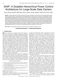
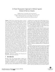
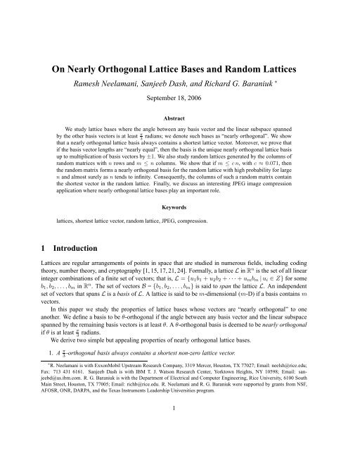
(1,2)(1,1.5)90 deg60 deg(0,0)(a)(0,0)(b)Figure 1: (a) The vectors comprising the lattice are denoted by circles. One of the lattice bases comprises twoorthogonal vectors of lengths 1 and 1.5. Since 1.5 < η ( ) √π2 = 3, the lattice possesses no other basis such that theangle between its vectors is at least π 3 radians. (b) This lattice contains at least two π 3-orthogonal bases. One of thelattice bases comprises two orthogonal vectors of lengths 1 and 2. Here 2 > η ( )π2 , and this basis is not the only-orthogonal basis.π3Theorem 2 Let B = (b 1 ,b 2 ,... ,b m ) be a weakly θ-orthogonal basis for a lattice L with θ > π 3. For alli ∈ {1,2,... ,m}, if‖b i ‖ < η(θ) min ‖b j‖ , (6)j∈{1,2,...,m}√3with η(θ) =sin θ + √ 3 cos θ , (7)then any π 3-orthogonal basis comprises the vectors in B multiplied by ±1.In other words, a nearly orthogonal basis is essentially unique when the lengths of its basis vectors are nearlyequal. For example, both Fig. 1(a) and (b) illustrate 2-D lattices that can be spanned by orthogonal basisvectors. For the lattice in Fig. 1(a), the ratio of the lengths of the basis vectors is less than η ( √π2)= 3.Hence, there exists only one (modulo sign changes) basis such that the angle between the vectors is greaterthan π 3 . In contrast, the lattice in Fig. 1(b) contains many distinct π 3-orthogonal bases.In the JPEG CHEst application [23], the target 3-D lattice bases in R 3 are known to be weakly ( π3 + ɛ) -orthogonal but not ( π3 + ɛ) -orthogonal. Theorem 2 addresses the uniqueness of π 3-orthogonal bases, but notweakly π 3-orthogonal bases. To estimate the target lattice basis, we need to understand how different weaklyorthogonal bases are related. The following theorem guarantees that for 3-D lattices, a weakly ( π3 + ɛ) -orthogonal basis with nearly equal-length basis vectors is related to every weakly orthogonal basis by aunimodular matrix with small entries.Theorem 3 Let B = (b 1 ,b 2 ,...,b m ) and ˜B be two weakly θ-orthogonal bases for a lattice L, where θ > π 3 .Let U = (u ij ) be a unimodular matrix such that B = ˜BU. Defineκ(B) =Then, |u ij | ≤ κ(B), for all i and j.( 2 √3) m−1× max i∈{1,2,...,m} ‖b i ‖min i∈{1,2,...,m} ‖b i ‖ . (8)For example, if B is a weakly θ-orthogonal basis of a 3-D lattice with max i∈{1,2,3}‖b i ‖min i∈{1,2,3} ‖b i ‖< 1.5, then the entriesof the unimodular matrix relating another weakly θ-orthogonal basis ˜B to B are either 0 or ±1.5

4 Nearly Orthogonal Bases: Proofs4.1 Proof of Theorem 1We first prove Theorem 1 for 2-D lattices (Gauss’s result) and then tackle the proof for higher-dimensionallattices via induction.4.1.1 Proof for 2-D latticesConsider a 2-D lattice with a basis B = {b 1 ,b 2 } satisfying the conditions of Theorem 1. Let θ ′ denote theangle between b 1 and b 2 . Since π 3 ≤ θ′ ≤ π 2by assumption,|〈b 1 ,b 2 〉| = ‖b 1 ‖ ‖b 2 ‖cos θ ′ ≤ ‖b 1‖ ‖b 2 ‖. (9)2The squared-length of any non-zero lattice vector v = u 1 b 1 + u 2 b 2 , with u 1 ,u 2 ∈ Z and |u 1 | + |u 2 | > 0,equals‖v‖ 2 = |u 1 | 2 ‖b 1 ‖ 2 + |u 2 | 2 ‖b 2 ‖ 2 + 2u 1 u 2 〈b 1 ,b 2 〉≥ |u 1 | 2 ‖b 1 ‖ 2 + |u 2 | 2 ‖b 2 ‖ 2 − 2|u 1 ||u 2 ||〈b 1 ,b 2 〉|≥ |u 1 | 2 ‖b 1 ‖ 2 + |u 2 | 2 ‖b 2 ‖ 2 − |u 1 ||u 2 |‖b 1 ‖ ‖b 2 ‖ (using (9))= (|u 1 |‖b 1 ‖ − |u 2 |‖b 2 ‖) 2 + |u 1 ||u 2 |‖b 1 ‖ ‖b 2 ‖ (10)≥ min ( ‖b 1 ‖ 2 , ‖b 2 ‖ 2) ,with equality possible only if either |u 1 | + |u 2 | = 1 or θ ′ = π 3. This proves Theorem 1 for 2-D lattices.4.1.2 Proof for higher-dimensional latticesLet k > 2 be an integer, and assume that Theorem 1 is true for every (k−1)-D lattice. Consider a k-D latticeL spanned by a weakly ( π3 + ɛ) -orthogonal basis (b 1 ,b 2 ,... ,b k ), with ɛ ≥ 0. Any non-zero vector in L canbe written as ∑ ki=1 u i b i for integers u i , where u i ≠ 0 for some i ∈ {1,2,... ,k}. If u k = 0, then ∑ ki=1 u i b iis contained in the (k − 1)-D lattice spanned by the weakly ( π3 + ɛ) -orthogonal basis (b 1 ,b 2 ,... ,b k−1 ). Foru k = 0, by the induction hypothesis, we have∥ ∥∥ ∥ k∑ ∥∥∥∥ ∑k−1∥∥∥∥ u∥ i b i =u∥ i b i ≥i=1i=1min ‖b j‖ ≥j∈{1,2,...,k−1}min ‖b j‖.j∈{1,2,...,k}If ɛ > 0, then the first inequality in the above expression can hold as equality only if ∑ k−1i=1 |u i| = 1. Ifu k ≠ 0 and u i = 0 for i = 1,2,... ,k − 1, then again∥∥ k∑ ∥∥∥∥ u∥ i b i ≥ ‖b k ‖ ≥i=1min ‖b j‖ .j∈{1,2,...,k}Again, it is necessary that |u k | = 1 for equality to hold above.Assume that u k ≠ 0 and u i ≠ 0 for some i ∈ {1,2,... ,k − 1}. Now ∑ ki=1 u i b i is contained in the 2-Dlattice spanned by the vectors ∑ k−1i=1 u i b i and u k b k . Since the ordered set (b 1 ,b 2 ,... ,b k ) is weakly ( π3 + ɛ) -orthogonal, the angle between the non-zero vectors ∑ k−1i=1 u i b i and u k b k lies in the interval [ π3 + ɛ, π 2].6

Invoking Theorem 1 for 2-D lattices, we have∥ (∥ ∥ )k∑ ∥∥∥∥ ∥∥∥∥ ∑k−1∥∥∥∥ u i b i ≥ min u i b i , ‖u∥k b k ‖i=1i=1()≥ min min ‖b j‖, ‖u k b k ‖j∈{1,2,...,k−1}≥min ‖b j‖ . (11)j∈{1,2,...,k}Thus, the set of basis vectors {b 1 ,b 2 ,... ,b k } contains a shortest non-zero vector in the k-D lattice. Also, ifɛ > 0, then equality is not possible in (11), and the second part of the theorem follows.✷4.2 Proof of Theorem 2Similar to the proof of Theorem 1, we first prove Theorem 2 for 2-D lattices and then prove the general caseby induction.4.2.1 Proof for 2-D latticesConsider a 2-D lattice in R n with basis vectors b 1 and b 2 such that the basis {b 1 ,b 2 } is weakly θ-orthogonalwith θ > π 3. Note that for 2-D lattices, weak θ-orthogonality is the same as θ-orthogonality. Without lossof generality (w.l.o.g.), we can assume that 1 = ‖b 1 ‖ ≤ ‖b 2 ‖. Further, by rotating the 2-D lattice, the basisvectors can be expressed as the columns of the n × 2 matrix⎡ ⎤1 b 210 b 220 0.⎢ ⎥⎣ . . ⎦0 0Let θ ′ ∈ [ θ, π 2]denote the angle between b1 and b 2 . Clearly,Since (6) holds by assumption,‖b 2 ‖

{˜b1 ,˜b 2}contain a common shortest lattice vector. Assume w.l.o.g. that˜b 1 = ±b 1 is a shortest lattice vector.Then, we can write[˜b1 ˜b2]= [ ] [ ]±1 ub 1 b 20 ±1To prove Theorem 2, we need to show that u = 0.Let ˜θ denote the angle between ˜b 1 and ±˜b 2 . Then,If u ≠ 0, thenHence,Therefore, from (13) we have∣ ∣∣〈˜b1 ,˜b 2 〉 ∣ 2cos 2 ˜θ = ∥∥ ∥∥2 ∥ ∥ ∥∥2∥˜b 1 ∥˜b2=>=with u ∈ Z.(u ± b 21 ) 2(u ± b 21 ) 2 + b 2 22(u ± b 21 ) 2(u ± b 21 ) 2 + 3(1 − |b 21 |) 2 (using (12))11 + 3(1−|b . (13)21|) 2(u±b 21 ) 2|u ± b 21 | ≥ |u| − |b 21 | ≥ 1 − |b 21 | ≥ 0 (from (12)).|u ± b 21 | 2 ≥ (1 − |b 21 |) 2 .cos 2 ˜θ >14 , (14)which holds if and only if ˜θ}< π 3{˜b1 . Thus, ,˜b 2 can be π 3-orthogonal only if u = 0. This proves Theorem 2for 2-D lattices.4.2.2 Proof for higher-dimensional latticesLet B and ˜B be two n × k matrices defining bases of the same k-D lattice in R n . We can write B = ˜B Ufor some integer unimodular matrix U = (u ij ). Using induction on k, we will show that if B is weaklyθ-orthogonal with π 3 < θ ≤ π 2 , if the columns of B satisfy (6), and if ˜B is π 3 -orthogonal, then ˜B can beobtained by permuting the columns of B and multiplying them by ±1. Equivalently, we will show everycolumn of U has exactly one component equal to ±1 and all others equal to 0 (we call such a matrix a signedpermutation matrix).Assume that Theorem 2 holds for all (k − 1)-D lattices with k > 2. Let b 1 ,b 2 ,...,b k denote thecolumns of B and let ˜b 1 ,˜b 2 ,...,˜b k denote the columns of ˜B. Since permuting the columns of ˜B does notdestroy π 3 -orthogonality, we can assume w.l.o.g. that ˜b 1 is ˜B’s shortest vector. From Theorem 1, ˜b 1 is alsoa shortest lattice vector. Further, using Corollary 1, ±˜b 1 is contained in B. Assume that b l = ±˜b 1 for some8

l ∈ {1,2,... ,k}. Then⎡⎤u 11 ... u 1l−1 ±1 u 1l+1 ... u 1kB = ˜B.⎢⎣ U 1 ′ 0 U 2′ ⎥⎦.(15)Above, U 1 ′ is a (k − 1) × (l − 1) sub-matrix, where as U 2 ′ is a (k − 1) × (k − l) sub-matrix. We will showthat u 1j = 0, for all j ∈ {1,2,... ,k} with j ≠ l. DefineB r = [ ] [∑]b l b j , ˜Br = k ˜b1i=2 u ij˜b i . (16)Then, from (15) and (16),B r = ˜B r[ ±1 u1j0 1].Since B r and ˜B r are related by a unimodular matrix, they both define bases of the same 2-D lattice. Further,B r is weakly θ-orthogonal with ||b j || < η(θ)||b l ||, and ˜B r is π 3-orthogonal. Invoking Theorem 2 for 2-Dlattices, we can infer that u 1j = 0. It remains to be shown that U ′ = [U 1 ′ U 2 ′ ] is also a signed permutationmatrix, whereB ′ = ˜B ′ U ′ ,with B ′ = [b 1 ,b 2 ,...,b l−1 , b l+1 ,... ,b k ] and ˜B]′ =[˜b2 ,˜b 3 ,...,˜b k . Observe that det(U ′ ) = det(U) = ±1.Both B ′ and ˜B ′ are bases of the same (k − 1)-D lattice as U ′ is unimodular. ˜B′ is π 3-orthogonal, whereas B′is weakly θ-orthogonal and its columns satisfy (6). By the induction hypothesis, U ′ is a signed permutationmatrix. Therefore, U is also a signed permutation matrix.✷4.3 Proof of Theorem 3Theorem 3 is a direct consequence of the following lemma.Lemma 1 Let B = (b 1 ,b 2 ,...,b m ) be a weakly θ-orthogonal basis of a lattice, where θ > π 3. Then, forany integers u 1 ,u 2 ,...,u m ,∥ m∑ ∥∥∥∥(√ ) m−13u∥ i b i ≥× max2‖u ib i ‖. (17)i∈{1,2,...,m}i=1Lemma 1 can be proved as follows. Consider the vectors b 1 and b 2 ; the angle θ between them lies in theinterval ( π3 , π 2). Recall from (10) that‖u 1 b 1 + u 2 b 2 ‖ 2 ≥ (|u 1 | ‖b 1 ‖ − |u 2 | ‖b 2 ‖) 2 + |u 1 ||u 2 |‖b 1 ‖‖b 2 ‖.Consider the expression (y − x) 2 + yx with 0 ≤ x ≤ y. For fixed y this expression attains its minimumvalue of ( 34)y 2 when x = y 2 . By setting y = |u 1| ‖b 1 ‖ and x = |u 2 | ‖b 2 ‖ w.l.o.g, we can infer that√3‖u 1 b 1 + u 2 b 2 ‖ ≥ max2‖u ib i ‖.i∈{1,2}9

Since B is weakly θ-orthogonal, the angle between u k b k and ∑ k−1i=1 u ib i lies in the interval ( π3 , π 2)fork = 2,3,... ,m. Hence (17) follows by induction.✷( √3 ) m−1.We now proceed to prove Theorem 3 by invoking Lemma 1. Define ∆ =For any j ∈{1,2,... ,m}, we have∥ m∑ ∥∥∥∥‖b j ‖ =u∥ ij˜bi ≥ ∆i=1maxi∈{1,2,...,m}∥∥ ∥∥∥u ij˜bi ≥ ∆ min ‖˜b i ‖ max |u ij|.i∈{1,2,...,m} i∈{1,2,...,m}Since B and ˜B are both weakly θ-orthogonal with θ > π 3 , min i∈{1,2,...,m} ‖˜b i ‖ = min i∈{1,2,...,m} ‖b i ‖.Therefore,∆ max |u ij| ≤i∈{1,2,...,m}‖b j ‖min i∈{1,2,...,m} ‖˜b i ‖ ≤ max i∈{1,2,...,m} ‖b i ‖min i∈{1,2,...,m} ‖b i ‖ = ∆κ(B).2Thus, |u ij | ≤ κ(B), for all i and j.✷5 Random Lattices and SVPIn several applications, the orthogonality of random lattice bases and the length of the shortest vector λ(L)in a random lattice L play an important role. For example, in certain wireless communications applicationsinvolving multiple transmitters and receivers, the received message ideally lies on a lattice spanned by arandom basis [7]. The random basis models the fluctuations in the communication channel between eachtransmitter-receiver pair. Due to the presence of noise, the ideal received message is retrieved by solving aCVP. The complexity of this problem is controlled by the orthogonality of the random basis [1]. Randombases are also employed to perform error correction coding [28] and in cryptography [28]. The level ofachievable error correction is controlled by the shortest vector in the lattice.In this section, we determine the θ-orthogonality of random bases. This result immediately lets usidentify conditions under which a random basis contains (with high probability) the shortest lattice vector.Before describing our results on random lattices and bases, we first review some known properties ofrandom lattices and then list some powerful results from random matrix theory.5.1 Known Properties of Random LatticesConsider an m-D lattice generated by a random basis with each of the m basis vectors chosen independentlyand uniformly from the unit ball in R n (n ≥ m). 2 With m fixed and with n → ∞, the probability that therandom basis is Minkowski-reduced tends to 1 [11]. Thus, as n → ∞, the random basis contains a shortestvector in the lattice almost surely. Recently, [3] proved that as n − m → ∞, the probability that a randombasis is LLL-reduced → 1. [3] also showed that a random basis is LLL-reduced with non-zero probabilitywhen n − m is fixed with n → ∞.5.2 Known Properties of Random MatricesRandom matrix theory, a rich field with many applications [6, 12], has witnessed several significant developmentsover the past few decades [12, 18, 19, 30]. We will invoke some of these results to derive some2 The m vectors form a basis because they are linearly independent almost surely.10

new properties of random bases and lattices; the paper [6] provides an excellent summary of the results wemention below.Consider an n × m matrix B with each element of B an independent identically distributed randomvariable. If the variables are zero-mean Gaussian distributed with variance 1 n, then we refer to such a B as aGaussian random basis. If the variables take on values in {− √ 1 1n, √n } with equal probability, then we termB to be a Bernoulli random basis. We denote the eigenvalues of B T B by ψi 2 , i = 1,2,... ,m. Gaussian andBernoulli random bases enjoy the following properties.1. For both Gaussian and Bernoulli B, B T B’s smallest and largest eigenvalues, ψmin 2 and ψ2 max, convergealmost surely to (1 − √ c) 2 and (1 + √ c) 2 respectively as n,m → ∞ and m n→ c < 1 [6, 12, 30].2. Let ɛ > 0 be given. Then, there exists an N ɛ such that for every n > N ɛ and r > 0,( ( √ ) ) mP |ψ min | ≤ 1 − − (r + ɛ) ≤ e − nr2ρ (18)n( ( √ ) ) mP |ψ max | ≥ 1 + + (r + ɛ) ≤ e − nr2ρ , (19)nwith ρ = 2 for Gaussian B and ρ = 16 for Bernoulli B [6, 18].In essence, a random matrix’s largest and smallest singular values converge, respectively, to 1 ± √ mn almostsurely as n,m → ∞ and lie close to 1 ± √ mnwith very high probability at finite (but sufficiently large) n.5.3 New Results on Random LatticesWe now formally state the new properties of random lattices mentioned in the Introduction plus severaladditional corollaries. The key step in proving these properties is to relate the condition number of a randombasis to its θ-orthogonality (see Lemma 2). A matrix’s condition number is defined as the ratio of the largestto the smallest singular value. Then we invoke the results in Section 5.2 to quantify the θ-orthogonality ofrandom bases. Finally we invoke previously deduced properties of nearly orthogonal lattice bases.We wish to emphasize that we prove our statements only for lattices which are not full-dimensional.Our computational results suggest these statements are not true for full-dimensional lattices. Further, Sorkin[31] proves that with high-probability, Gaussian random matrices are not nearly orthogonal when m > n/4.See the paragraph after Corollary 3 for more details.Lemma 2 Consider an arbitrary n × m real-valued matrix B, with m ≤ n, whose largest and smallestsingular values are denoted by ψ max and ψ min , respectively. Then the columns of B are θ-orthogonal with( )θ = sin −1 2ψmax ψ minψmin 2 + . (20)ψ2 maxThe proof is given in Section 5.4. The value of θ in (20) is the best possible in the sense that there is a 2 × 2matrix B with singular values ψ min and ψ max such that the angle between the two columns of B is given by(20). Note that for large ψ minψ max(that is, small condition number), the θ in (20) is close to π 2. Thus, Lemma 2quantifies our intuition that a matrix with small condition number should be nearly orthogonal.By combining Lemma 2 with the properties of random matrices listed in Section 5.2, we can immediatelydeduce the θ-orthogonality of an n × m random basis. See Section 5.4.2 for the proof.11

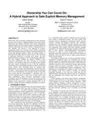
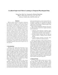
Theorem 4 Let B denote an n × m Gaussian or Bernoulli random basis. If m ≤ cn, 0 ≤ c < 1, then asn → ∞, B is θ-orthogonal almost surely with( ) 1 − cθ = sin −1 . (21)1 + cFurther, given an ɛ > 0, there exists an N ɛ such that for every n > N ɛ and r > 0, B is θ-orthogonal,()θ = sin −1 1 − c1 + c − 3√ 34 (r + ɛ) , (22)with probability greater than 1 − 2e − nr2ρ , where ρ = 2 for Gaussian B and ρ = 16 for Bernoulli B.The value of θ in (21) is not the best possible in the sense that for a given value of c, a random n×m Gaussianmatrix with m ≤ cn would be θ ′ -orthogonal (with high probability) for some θ ′ > θ (see Figure 2). Thereason is that the θ predicted by Lemma 2 is satisfied by all matrices. However, Theorem 4 is restricted torandom matrices.Theorem 4 allows us to bound the length of the shortest non-zero vector in a random lattice.Corollary 2 Let the n × m-matrix B = (b 1 ,b 2 ,... ,b m ), with m ≤ cn and 0 ≤ c < 1, denote a Gaussianor Bernoulli random basis for a lattice L. Then the shortest vector’s length λ(L) satisfiesalmost surely as n → ∞.λ(L) ≥ 1 − c1 + cEach column of a Bernoulli B is unit-length by construction. For Gaussian B, it is not difficult to show thatall columns have length 1 almost surely as n → ∞. Hence Corollary 2 is an immediate consequence ofTheorem 4 and (2). Corollary 2 implies that in random lattices that are not full-dimensional, it is easy toobtain approximate solutions to the SVP (within a constant factor). This is because for random lattices in R nwith dimension n(1−ɛ), λ(L) is greater than ɛ times the length of the shortest basis vector (approximately).Compare this with Daudé and Vallée’s [9] result that in random full-dimensional lattices in R n , λ(L) is atleast O(1/ √ n) times the length of the shortest basis vector with high probability.By substituting θ = π 3into Theorem 4 and then invoking Corollary 1, we can deduce sufficient conditionsfor a random basis to be π 3 -orthogonal.Corollary 3 Let the n × m-matrix B denote a Gaussian or Bernoulli random basis for lattice L. If m n ≤c < ( 7 − √ 48 ) (≈ 0.071), then B is π 3-orthogonal almost surely as n → ∞. Further, given an ɛ > 0, thereexists an N ɛ such that for every n > N ɛ and4(1−c)3 √ − ɛ − 2 3(1+c) 3 > r > 0, B is π 3-orthogonal with probabilitygreater than 1 − 2e − nr2ρ , where ρ = 2 for Gaussian B and ρ = 16 for Bernoulli B.Figure 2 illustrates that, in practice, an n×m Gaussian and Bernoulli random matrix is nearly orthogonalfor much larger values of m nthan our results claim. Our plots suggest that the probability for a random basisto be nearly orthogonal sharply transitions from 1 to 0 for m nvalues in the interval [0.2,0.25]. Sorkin [31]has shown us that if the columns of B represent points chosen uniformly from the unit sphere in R n (onecan obtain such points by dividing the columns of a Gaussian matrix by their norms), then the best possiblemn value for random n × m matrices to be π 3 -orthogonal is m n= 0.25. Further, if m/n > 0.25, B is almostsurely not π 3-orthogonal as n → ∞. For large n, the columns of a Gaussian matrix almost surely have length1, and thus behave like points chosen uniformly from the unit sphere in R n . Therefore, as n → ∞, randomn × n/4 Gaussian matrices are almost surely π 3 -orthogonal.12

5.4 Proof of Results on Random LatticesThis section provides the proofs for Lemma 2 and Theorem 4.5.4.1 Proof of Lemma 2Our goal is to construct a lower-bound for the angle between any column of B and the subspace spanned byall the other columns in terms of the singular values of B. Clearly, if ψ min = 0, then the columns of B arelinearly dependent. Hence, (20) holds as B’s columns are θ-orthogonal with θ = 0. For the rest of the proof,we will assume that ψ min ≠ 0.Consider the singular value decomposition (SVD) of BB = XΨY, (23)where X and Y are n × m and m × m real-valued matrices respectively with orthonormal columns, and Ψis a m × m real-valued diagonal matrix. Let b i and x i denote the i-th column of B and X respectively, lety ij denote the element from the i-th row and j-th column of Y, and let ψ i denote the i-th diagonal elementof Ψ. Then, (23) can be rewritten as⎡⎤ ⎡⎤ψ 1 0 ... 0 y 11 y 12 ... y 1m[ ] [ ]0 ψ 2 ... 0y 21 y 22 ... y 2mb1 b 2 ... b m = x1 x 2 ... x m ⎢⎣.. ..⎥ ⎢. ⎦ ⎣.. ..⎥. ⎦ .0 ... ... ψ m y m1 ... ... y mmWe now analyze the angle between b 1 (w.l.o.g) and the subspace spanned by {b 2 ,b 3 ,... ,b m }. Note thatb 1 =m∑ψ i y i1 x i .i=1Let ˜b 1 denote an arbitrary non-zero vector in the subspace spanned by {b 2 ,b 3 ,... ,b m }. Then,˜b1 =m∑α k b k =m∑k=2 k=2α km ∑i=1ψ i y ik x i =m∑x i ψ ii=1m ∑k=2α k y ik .for some α k ∈ R with ∑ k |α k| > 0. Let ỹ i1 = ∑ mk=2 α k y ik . Then,˜b1 =m∑ψ i ỹ i1 x i .i=1Let ˜θ ≥ θ denote the angle between b 1 and ˜b 1 . Then,〈 〉∣ ∣∣cos ˜θ∣ b 1 ,˜b 1=∥∥ ∥∥= |〈∑ mi=1 ψ i y i1 x i , ∑ mi=1 ψ i ỹ i1 x i 〉|‖b 1 ‖ ∥˜b ‖ ∑ m1 i=1 ψ i y i1 x i ‖ ‖ ∑ mi=1 ψ (24)i ỹ i1 x i ‖∣ ∑ mi=1=ψ2 i y ∣i1 ỹ i1 , (25)√ ∑mi=1 ψ2 i y2 i1√ ∑mi=1 ψ2 i ỹ2 i113

where the orthonormality of X ’s columns is used to obtain (25) from (24). Let y i , i = 1,2,... ,m, and ỹ 1denote column vectors⎡ ⎤ ⎡ ⎤y 1iỹ 11y 2iy i := ⎢ ⎥⎣ . ⎦ and ỹ ỹ 211 := ⎢ ⎥⎣ . ⎦ .y mi ỹ m1Since ỹ 1 = ∑ mk=2 α k y k ,ỹ T 1 y 1 = 0.Then (25) can be rewritten using matrix notation as∣cos ˜θ∣ yT= 1 Ψ 2 ỹ 1 , (26)√y1 TΨ2 y 1√ỹ1 TΨ2 ỹ 1with Ψ 2 := Ψ T Ψ. The angle ˜θ is minimized when the right hand side of (26) is maximized.For arbitrary B with only the singular values known (that is, Ψ is known), the θ-orthogonality of B isgiven by solving the following constrained optimization problem.cos θ = maxy 1 ,ey 1∣ ∣y T1 Ψ 2 ỹ 1∣ ∣√y T 1 Ψ2 y 1√ỹ T 1 Ψ2 ỹ 1, such that ỹ T 1 y 1 = 0. (27)Wielandt’s inequality [14, Thm. 7.4.34] states that if A is a positive definite matrix, with γ min and γ maxdenoting its minimum and maximum eigenvalues (both are positive), then|x T Ay| 2 ≤(γmax − γ minγ max + γ min) 2(x T Ax)(y T Ay)for every pair of orthogonal vectors x and y (equality holds for some pair of orthogonal vectors). In ourproblem, A = Ψ 2 , x = ỹ 1 , y = y 1 , γ max = ψmax 2 and γ min = ψmin 2 . Therefore, using Wielandt’s inequalityand (27), we haveHencewhich proves (20).5.4.2 Proof of Theorem 4cos θ = ψ2 max − ψmin2ψmax 2 + ψmin2 .sin θ = 2ψ maxψ minψmax 2 + , (28)ψ2 min✷The first part of Theorem 4 follows easily. From Section 5.2, we can infer that with m ≤ cn, 0 ≤ c < 1,both ψ min ≥ 1 − √ c and ψ max ≤ 1 + √ c almost surely as n → ∞. Invoking Lemma 2 and substitutingψ min = 1 − √ c and ψ max = 1 + √ c into (20), it follows that as n → ∞, B is θ-orthogonal almost surelywith θ given by (21).14

We now focus on proving the second part of Theorem 4. Let d = √ c, and defineWe first show that for δ ≥ 0,G(d) := 1 − d21 + d 2.G(d + δ) ≥ G(d) − 3√ 3δ. (29)4Using the mean value theorem,(G(d + δ) = G(d) + G ′ d + ˜δ)δ, for some ˜δ ∈ (0,δ), (30)with G ′ denoting the derivative of G with respect to d. Further,G ′ (d) =−4d(1 + d 2 ) 2 ≥ −3√ 3, for d > 0. (31)4One can verify the inequality above by differentiating G ′ (d), and observing that G ′ (d) is minimized when3d 4 + 2d 2 − 1 = 0. The only positive root of this quadratic equation is d 2 = 1/3 or d = 1/ √ 3. Combining(30) and (31), we obtain (29).From the results in Section 5.2, it follows that the probability that both minimum and maximum singularvalues of B satisfy|ψ min | ≥ 1 − (√ c + r + ɛ ) and |ψ max | ≤ 1 + (√ c + r + ɛ ) (32)is greater than 1 − 2e − nr2ρ . When (32) holds, B is at least sin −1 (G( √ c + r + ɛ))-orthogonal. This followsfrom (20). Invoking (29), we can infer that B is θ-orthogonal with θ as in (22).✷6 JPEG Compression History Estimation (CHEst)In this section, we review the JPEG CHEst problem that motivates our study of nearly orthogonal lattices,and describe how we use this paper’s results to solve this problem. We first touch on the topic of digitalcolor image representation and briefly describe the essential components of JPEG image compression.6.1 Digital Color Image RepresentationTraditionally, digital color images are represented by specifying the color of each pixel, the smallestunit of image representation. According to the trichromatic theory [29], three parameters are sufficientto specify any color perceived by humans. 3 For example, a pixel’s color can be conveyed by a vectorw RGB= (w R,w G,w B) ∈ R 3 , where w R, w G, and w Bspecify the intensity of the color’s red (R), green (G),and blue (B) components respectively. Call w RGBthe RGB encoding of a color. RGB encodings are vectorsin the vector space where the R, G, and B colors form the standard unit basis vectors; this coordinate systemis called the RGB color space. A color image with M pixels can be specified using RGB encodings by amatrix P ∈ R 3×M .3 The underlying reason is that the human retina has only three types of receptors that influence color perception.15

6.2 JPEG Compression and DecompressionTo achieve color image compression, schemes such as JPEG first transform the image to a color encodingother than the RGB encoding and then perform quantization. Such color encodings can be related to theRGB encoding by a color-transform matrix C ∈ R 3×3 . The columns of C form a different basis for thecolor space spanned by the R, G, and B vectors. Hence an RGB encoding w RGBcan be transformed to theC encoding vector as C −1 w RGB; the image P is mapped to C −1 P . For example, the matrix relating theRGB color space to the ITU.BT-601 Y CbCr color space is given by [27]⎡ ⎤ ⎡⎤ ⎡ ⎤w Y0.299 0.587 0.114 w R⎣w Cb⎦ = ⎣−0.169 −0.331 0.5 ⎦ ⎣w G⎦. (33)w Cr0.5 −0.419 −0.081 w BThe quantization step is performed by first choosing a diagonal, positive (non-zero entries are positive),integer⌈quantization matrix Q, and then computing the quantized (compressed) image from C −1 P as P c =Q −1 C −1 P ⌋ , where ⌈.⌋ stands for the operation of rounding to the nearest integer. JPEG decompressionconstructs P d = CQP c = CQ ⌈ Q −1 C −1 P ⌋ . Larger Q’s achieve more compression but at the cost ofgreater distortion between the decompressed image P d and the original image P .In practice, the image matrix P is first decomposed into different frequency components P ={P 1 , P 2 , ... ,P k }, for some k > 1 (usually k = 64), during compression. Then, a commoncolor transform C is applied to all the sub-matrices P 1 , P 2 , ... ,P k , but each sub-matrixP i is quantized with a different quantization matrix Q i . The compressed image is P c ={P c,1 ,P c,2 ,...,P c,k } = {⌈ Q −1 ⌋ ⌈ ⌋ ⌈ ⌋}1 C−1 P 1 , Q−12 C−1 P 2 ,... , Q−1k C−1 P k , and the decompressed imageis P d = {CQ 1 P c,1 ,CQ 2 P c,2 ,...,CQ k P c,k }.During compression, the JPEG compressed file format stores the matrix C and the matrices Q i ’s alongwith P c . These stored matrices are utilized to decompress the JPEG image, but are discarded afterward.Hence we refer to the set {C,Q 1 ,Q 2 ,... ,Q k } as the compression history of the image.6.3 JPEG CHEst Problem StatementThis paper’s contributions are motivated by the following question: Given a decompressed image P d ={CQ 1 P c,1 ,CQ 2 P c,2 ,... ,CQ k P c,k } and some information about the structure of C and the Q i ’s, can weestimate the color transform C and the quantization matrices Q i ’s? As {C,Q 1 ,Q 2 ,... ,Q k } comprisesthe compression history of the image, we refer to this problem as JPEG CHEst. An image’s compressionhistory is useful for applications such as JPEG recompression [5, 22, 23].6.4 Near-Orthogonality and JPEG CHEstThe columns of CQ i P c,i lie on a 3-D lattice with basis CQ i because P c,i is an integer matrix. The estimationof CQ i ’s comprises the main step in JPEG CHEst. Since a lattice can have multiple bases, wemust exploit some additional information about practical color transforms to correctly deduce the CQ i ’sfrom the CQ i P c,i ’s. Most practical color transforms aim to represent a color using an approximately rotatedreference coordinate system. Consequently, most practical color transform matrices C (and thus, CQ i ) canbe expected to be almost orthogonal. We have verified that all C’s used in practice are weakly ( π3 + ɛ) -orthogonal, with 0 < ɛ ≤ π 6 .4 Thus, nearly orthogonal lattice bases are central to JPEG CHEst.4 In general, the stronger assumption of π -orthogonality does not hold for some practical color transform matrices.316

6.5 Our ApproachOur approach is to first estimate the products CQ i by exploiting the near-orthogonality of C and to thendecompose CQ i into C and Q i . We will assume that C is weakly ( π3 + ɛ) -orthogonal, 0 < ɛ ≤ π 6 .6.5.1 Estimating the CQ i ’sLet B i be a basis of the lattice L i spanned by CQ i . Then, for some unimodular matrix U i , we haveB i = CQ i U i . (34)If B i is given, then estimating CQ i is equivalent to estimating the respective U i .Thanks to our problem structure, the correct U i ’s satisfy the following constraints. Note that theseconstraints become increasingly restrictive as the number of frequency components k increases.1. The U i ’s are such that B i U −1iis weakly ( π3 + ɛ) -orthogonal.2. The product U i Bi−1 B j Uj−1 is diagonal with positive entries for any i,j ∈ {1,2,... ,k}.This is an immediate consequence of (34).If in addition, B i is weakly ( π3 + ɛ) -orthogonal, then3. The columns of U i corresponding to the shortest columns of B i are the standard unit vectors times ±1.This follows from Corollary 1 because the columns of both B i and CQ i indeed contain all shortestvectors in L i up to multiplication by ±1.4. All entries of U i are ≤ κ(B i ) in magnitude.This follows from Theorem 3.We now outline our heuristic.(i) Obtain bases B i for the lattices L i , i = 1,2,... ,k. Construct a weakly ( π3 + ɛ) -orthogonal basis B lfor at least one lattice L l , l ∈ {1,2,... ,k}.(ii) Compute κ(B l ).(iii) For every unimodular matrix U l satisfying constraints 1, 3 and 4, go to step (iv).(iv) For U l chosen in step (iii), test if there exist unimodular matrices U j for each j = 1,2,... ,k,j ≠ lthat satisfy constraint 2. If such a collection of matrices exists, then return this collection; otherwisego to step (iii).For step (i), we simply use the LLL algorithm to compute LLL-reduced bases for each L i . Such basesare not guaranteed to be weakly ( π3 + ɛ) -orthogonal, but in practice, this is usually the case for a number ofthe L i ’s. Instead of LLL, the method proposed in [25] could be also employed (as suggested by the referees).In contrast to the LLL, [25] always finds a basis that contains the shortest lattice vector in low-dimensionallattices (up to 4-D) such as the L i ’s in our problem. In step (iv), for each frequency component j ≠ l, wecompute the diagonal matrix D j with smallest positive entries such that Ũj = Bj−1 B l U −1lD j is integral, andthen test whether Ũj is unimodular. If not, then for the given U l , no appropriate unimodular matrix U j exists.The overall complexity of the heuristic is determined mainly by the number of times we repeat step(iv), which equals the number of distinct choices for U l in step (iii). This number is typically not very large17

Table 1: Number of unimodular matrices satisfying constraints 3 and 4 for small κ.κ constraint 4 constraints 3 and 41 6960 52322 135408 432483 1281648 1976164 5194416 5132645 20852976 1324272because in step (i), we are usually able to find some weakly ( π3 + ɛ) -orthogonal basis B l with κ < 2. In fact,we enumerate all unimodular matrices satisfying constraints 3 and 4 and then test constraint 1. (In practice,one can avoid enumerating the various column permutations of a unimodular matrix). Table 1 providesthe number of unimodular matrices satisfying constraint 4 alone and also constraints 3 and 4. Clearly,constraints 3 and 4 help us to significantly limit the number of unimodular matrices we need to test, therebyspeeding up our search.Our heuristic returns a collection of unimodular matrices {U i } that satisfy constraints 1 and 2; of course,they also satisfy constraints 3 and 4 if the corresponding B i ’s are weakly ( π3 + ɛ) -orthogonal. From theU i ’s, we compute CQ i = B i U −1 . If constraints 1 and 2 can be satisfied by another solution {U i ′ }, then itis easy to see that U i ′ ≠ U i for every i = 1,2,... ,k. In Section 6.5.3, we will argue (without proof) thatconstraints 1 and 2 are likely to have a unique solution in most practical cases.6.5.2 Splitting CQ i into C and Q iDecomposing the CQ i ’s into C and Q i ’s is equivalent to determining the norm of each column of C becausethe Q i ’s are diagonal matrices. Since the Q i ’s are integer matrices, the norm of each column of CQ i is aninteger multiple of the corresponding column norm of C. In other words, the norms of the j-th column(j ∈ {1,2,3}) of different CQ i ’s form a sub-lattice of the 1-D lattice spanned by the j-th column norm ofC. As long as the greatest common divisor of the j-th diagonal values of the matrices Q i ’s is 1, we canuniquely determine the j-th column of C; the values of Q i follow trivially.6.5.3 UniquenessDoes JPEG CHEst have a unique solution ? In other words, is there a collection of matrices(C ′ ,Q ′ 1,Q ′ 2,...,Q ′ k ) ≠ (C,Q 1,Q 2 ,... ,Q k )such that C ′ Q ′ i is a weakly ( π3 + ɛ) -orthogonal basis of L i for all i ∈ {1,2,... ,k}? We believe thatthe solution can be non-unique only if the Q i ’s are chosen carefully. For example, let Q be a diagonalmatrix with positive diagonal coefficients. Assume that for i = 1,2,... ,k, Q i = α i Q, with α i ∈ R andα i > 0. Further, assume that there exists a unimodular matrix U not equal to the identity matrix I suchthat C ′ = CQU is weakly ( π3 + ɛ) -orthogonal. Define Q ′ i = α iI for i = 1,2,... ,k. Then C ′ Q ′ i is also aweakly ( π3 + ɛ) -orthogonal basis for L i . Typically, JPEG employs Q i ’s that are not related in any specialway. Therefore, we believe that for most practical cases JPEG CHEst has a unique solution.18

6.5.4 Experimental ResultsWe tested the proposed approach using a wide variety of test cases. In reality, the decompressed image P dis always corrupted with some additive noise. Consequently, to estimate the desired compression history,the approach described above was combined with some additional noise mitigation steps. Our algorithmprovided accurate estimates of the image’s JPEG compression history for all the test cases. We refer thereader to [22, 23] for details on the experimental setup and results.7 Discussion and ConclusionsIn this paper, we derived some interesting properties of nearly orthogonal lattice bases and random bases.We chose to directly quantify the orthogonality of a basis in terms of the minimum angle θ between a basisvector and the linear subspace spanned by the remaining basis vectors. When θ ≥ π 3radians, we say that thebasis is nearly orthogonal. A key contribution of this paper is to show that a nearly orthogonal lattice basisalways contains a shortest lattice vector. We also investigated the uniqueness of nearly orthogonal latticebases. We proved that if the basis vectors of a nearly orthogonal basis are nearly equal in length, then thelattice essentially contains only one nearly orthogonal basis. These results enable us to solve a fascinatingdigital color imaging problem called JPEG compression history estimation (JPEG CHEst).The applicability of our results on nearly orthogonal bases is limited by the fact that every lattice doesnot necessarily admit a nearly orthogonal basis. In this sense, lattices that contain a nearly orthogonal basisare somewhat special.However, in random lattices, nearly orthogonal bases occur frequently when the lattice is sufficientlylow-dimensional. Our second main result is that an m-D Gaussian or Bernoulli random basis that spans alattice in R n , with m < 0.071n, is nearly orthogonal almost surely as n → ∞ and with high probability atfinite but large n. Consequently, a random n × 0.071n lattice basis contains the shortest lattice vector withhigh probability. In fact, based on [31], the bound 0.071 can be relaxed to 0.25, at least in the Gaussian case.We believe that analyzing random lattices using some of the techniques developed in this paper is afruitful area for future research. For example, we have recently realized (using Corollary 3) that a randomn × 0.071n lattice basis is Minkowski-reduced with high probability [8].AcknowledgmentsWe thank Gabor Pataki for useful comments and for the reference to Gauss’s work in Vazirani’s book.We also thank the editor Alexander Vardy and the anonymous reviewers for their thorough and thoughtprovokingreviews; our work on random lattices was motivated by their comments. Finally, we thank GregorySorkin who gave us numerous insights into the properties of random matrices.References[1] E. Agrell, T. Eriksson, A. Vardy, and K. Zeger, “Closest point search in lattices,” IEEE Trans. Inform. Theory,vol. 48, pp. 2201–2214, Aug. 2002.[2] M. Ajtai, “The shortest vector problem in L 2 is NP-hard for randomized reductions,” in Proc. 30th annual ACMSymp. Theory of Computing, pp. 10–19, ACM Press, 1998.[3] A. Akhavi, J.-F. Marckert, and A. Rouault, “On the Lovász reduction of a random basis,” 2004.Submitted.19

[4] L. Babai, “On Lovász’ lattice reduction and the nearest lattice point problem,” Combinatorica, vol. 6, pp. 1–14,1986.[5] H. H. Bauschke, C. H. Hamilton, M. S. Macklem, J. S. McMichael, and N. R. Swart, “Recompression of JPEGimages by requantization,” IEEE Trans. Image Processing, vol. 12, pp. 843–849, Jul. 2003.[6] E. Candès and T. Tao, “Near optimal signal recovery from random projections and universal encoding strategies,”IEEE Trans. Inform. Theory, 2004. Submitted.[7] O. Damen, A. Chkeif, and J. Belfiore, “Lattice code decoder for space-time codes,” IEEE Commun. Lett.,pp. 161–163, May 2000.[8] S. Dash and R. Neelamani, “Some properties of SVP in random lattices”, 2006. Manuscript in preparation.[9] H. Daudé and B. Vallée, “An upper bound on the average number of iterations of the LLL algorithm,” TheoreticalComp. Sci., vol. 123, pp. 95-115, 1994.[10] I. Dinur, G. Kindler, R. Raz, and S. Safra, “Approximating CVP to within almost-polynomial factors is NP-hard,”Combinatorica, vol. 23, no. 2, pp. 205–243, 2003.[11] J. L. Donaldson, “Minkowski reduction of integral matrices,” Mathematics of Computation, vol. 33, no. 145,pp. 201—216, 1979.[12] N. El-Karoui, “Recent results about the largest eigenvalue of random covariance matrices and statistical applications,”Acta Physica Polonica B, vol. 36, no. 9, pp. 2681–2697, 2005.[13] C. F. Gauss, Disquisitiones Arithmeticae. New York: Springer-Verlag, English edition translated by A. A. Clark,1986.[14] R.A. Horn and C.R. Johnson, “Matrix Analysis,” Cambridge University Press, Cambridge, UK, 1985.[15] R. Kannan, “Algorithmic geometry of numbers,” Annual Review of Comp. Sci. vol. 2, pp. 231–267, 1987.[16] S. Khot, “Hardness of approximating the shortest vector problem in lattices,” J. ACM, vol. 52, pp. 789–808, Sept.2005. Preliminary version in FOCS 2004.[17] A. K. Lenstra, H. W. Lenstra, Jr., and L. Lovász, “Factoring polynomials with rational coefficients,” MathematischeAnnalen, vol. 261, pp. 515–534, 1982.[18] A.E. Litvak, A. Pajor, M. Rudelson and N. Tomczak-Jaegermann, “Singular values of random matrices andgeometry of random polytopes,” Advances in Mathematics, vol. 195, pp. 491–523, Aug. 2005.[19] V. A. Marchenko and L. A. Pastur, “Distribution of eigenvalues in certain sets of random matrices,” Mat. Sb.(N.S.), vol. 72, pp. 407–535, 1967. (in Russian).[20] D. Micciancio, “The shortest vector problem is NP-hard to approximate to within some constant,” SIAM J.Comp., vol. 30, pp. 2008–2035, 2001. Preliminary version in FOCS 1998.[21] D. Micciancio and S. Goldwasser, Complexity of lattice problems: A cryptographic perspective. Boston: KluwerAcademic, 2002.[22] R. Neelamani, Inverse Problems in Image Processing. Ph.D. dissertation, ECE Dept., Rice University, 2003.www.dsp.rice.edu/∼neelsh/publications/.[23] R. Neelamani, R. de Queiroz, Z. Fan, S. Dash, and R. G. Baraniuk, “JPEG compression history estimation forcolor images,” IEEE Trans. Image Processing, May 2006. To appear.[24] P. Nguyen and J. Stern, “Lattice reduction in cryptology: An update,” in Lecture notes in Comp. Sci., vol. 1838,pp. 85–112, Springer-Verlag, 2000.[25] P. Nguyen and D. Stehlé, “Low-dimensional lattice basis reduction revisited,” in Lecture Notes in Comp. Sci.,vol. 3076, pp. 338–357, Springer-Verlag, 2004.20

[26] W. Pennebaker and J. Mitchell, JPEG, Still Image Data Compression Standard. Van Nostrand Reinhold, 1993.[27] C. Poynton, A Technical Introduction to Digital Video. New York: Wiley, 1996.[28] O. Regev, “On lattices, learning with errors, random linear codes, and cryptography,” in Proc. 37th annual ACMSymp. Theory of Computing, (New York, NY, USA), pp. 84–93, ACM Press, 2005.[29] G. Sharma and H. Trussell, “Digital color imaging,” IEEE Trans. Image Processing, vol. 6, pp. 901–932, July1997.[30] J. W. Silverstein, “The smallest eigenvalue of a large dimensional Wishart matrix,” Ann. Probab., vol. 13,pp. 1364–1368, 1985.[31] G. Sorkin. Personal Communication. 2006.[32] V. V. Vazirani, Approximation Algorithms. Berlin: Springer-Verlag, 2001.21

110.80.8Probability0.60.4Probability0.60.40.2GaussianBernoulli00 0.05 0.1 0.15 0.2 0.25mn0.2GaussianBernoulli00 0.05 0.1 0.15 0.2 0.25mn(a) n = 256 (b) n = 512110.80.8Probability0.60.4Probability0.60.40.2GaussianBernoulli00 0.05 0.1 0.15 0.2 0.25mn0.2GaussianBernoulli00 0.05 0.1 0.15 0.2 0.25mn(c) n = 1024 (d) n = 2048Figure 2: Empirical probability that a n × m Gaussian or Bernoulli random matrix is π 3-orthogonal. Atn = 256, 512, 1024, and 2048 and at m indicated by circles (for Gaussian) and triangles (for Bernoulli),we tested 200 randomly generated matrices. The empirical probability is the fraction of random matricesthat were π 3 -orthogonal. 22