rtd, resistance temperature detector - Scientific Devices Australia

AN105 Dataforth Corporation Page 2 of 3
Rearranging this expression gives;
Resistance (V ÷ i) = [(ρ×L)÷A] , Ohms.
applied
Where ρ = 1/( e× n×µ
) and is the familiar parameter
“resistivity”, which characterizes resistance of any given
material. Note that since the electron charge “e” is a
constant, resistance is completely dominated and
controlled by the product of (n) electron density and (µ)
electron mobility. For most metals over a rather large
range of temperature, the (n x µ) product decreases with
increasing temperature; this increases resistance and
establishes a positive temperature coefficient. The number
of electrons and their complex interactive behavior
controls the resistance of materials.
The complex interactive behavior of billions of electrons
scrambling down a wire under the influence of
temperature and a forcing voltage creates a resistivity that
is seldom linear over all temperature. However, Copper,
Nickel, and Platinum do have near linear temperature
coefficients over certain ranges of temperature and,
therefore, are used in the manufacture of RTDs. Platinum
is the most linear.
RTD Model
RTD standards, define Platinum resistance vs temperature
behavior by the Callendar-Van Dusen equation, a nonlinear
mathematical model. These standards include; the
RTD value at 0 °C, R(0), equation coefficients, and a
temperature coefficient, alpha (α) defined from 0 to 100
°C. Alpha (α) can sometimes be used to establish a simple
linear model for resistance vs temperature. In addition,
different tolerance ranges identified as “classes” are
included within the associated standard’s information.
The Platinum RTD Callendar-Van Dusen non-linear
model is a forth order polynomial for negative
temperatures and a quadric for positive temperatures.
Cases 1, 2, 3 below show models for the RTD in the
general form of RTD = R(0) + ∆R, where ∆R is the
temperature dependent part of the RTD.
Measuring Temperature with RTDs
Temperature measurements with RTDs first electronically
measure the RTD resistance and then convert to
temperature using the RTD’s resistance vs temperature
characteristics. There are numerous circuit topologies
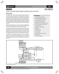
used to determine resistance. For example, Figure 1
illustrates a classic bridge configuration used for 3-wire
RTD measurements.
RTD
Rline3
Rline2
Rline1
Field Side
Rline1
R3
b
a
Module Side
R2
R1
Figure 1
The Classic 3-Wire RTD Bridge Topology
Vref
The voltage Vba in Figure 1 varies as RTD changes with
temperature. For R1 = R2 = R3 = R(0), equal Rlines, and
RTD defined as RTD = R(0) + ∆R then,
Vref ⎡ ∆R ⎤
Vba = ×
2
⎢
2R(0)+∆R+2Rline
⎥ .
⎣
⎦
Typical bridge output voltages (as shown above) include
line resistance and are non-linear.
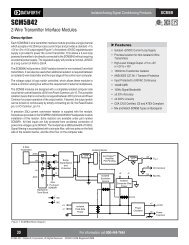
Modern semiconductor technology facilitates resistance
measurements with linear outputs and line resistances
eliminate. For example, Figure 2 illustrates a 4-wire RTD
configuration with current excitation.
Case (1) For T < 0; RTD = R(0) + ∆R
2 3
RTD = R (0) × [1 + A × T + B × T + C × ( T − 100) × T
] .
Case (2) For T > 0; RTD = R(0) + ∆R
RTD = R (0) × [1 + A × T + B × T
2
] .
RTD
Rline4
Rline3
Rline2
b
a
Iext
Case (3) The linear model is; RTD = R(0) + ∆R
RTD = R (0) × (1 + alpha × T
) .
Coefficients A, B, C, and alpha are defined by RTD
standards and measured by RTD manufacturers as
specified by these standards.
Field Side
Module Side
Figure 2
4-Wire RTD with Current Excitation