Measuring RMS Values of Voltage and Current - Scientific Devices ...
Measuring RMS Values of Voltage and Current - Scientific Devices ...
Measuring RMS Values of Voltage and Current - Scientific Devices ...

Create successful ePaper yourself
Turn your PDF publications into a flip-book with our unique Google optimized e-Paper software.
AN101 Dataforth Corporation Page 1 <strong>of</strong> 6<br />
DID YOU KNOW <br />
Gustav Robert Kirchh<strong>of</strong>f (1824-1887) the German Physicist who gave us "Kirchh<strong>of</strong>f's voltage (current) law"<br />
invented the Bunsen Burner working together with Robert Wilhelm Bunsen, a German Chemist.<br />
<strong>Measuring</strong> <strong>RMS</strong> <strong>Values</strong> <strong>of</strong> <strong>Voltage</strong> <strong>and</strong> <strong>Current</strong><br />
<strong>Voltage</strong> (<strong>Current</strong>) Measurements<br />
St<strong>and</strong>ard classic measurements <strong>of</strong> voltage (current)<br />
values are based on two fundamental techniques<br />
either "average" or "effective".<br />
The "average" value <strong>of</strong> a function <strong>of</strong> time is the net<br />
area <strong>of</strong> the function calculated over a specific<br />
interval <strong>of</strong> time divided by that time interval.<br />
Specifically,<br />
Vavg =<br />
F<br />
HG<br />
1<br />
T2 − T<br />
I K J z<br />
T2<br />
* Vtdt ( ) Eqn 1<br />
1 T1<br />
If a voltage (current) is either constant or periodic,<br />
then measuring its average is independent <strong>of</strong> the<br />
interval over which a measurement is made. If, on<br />
the other h<strong>and</strong>, the voltage (current) function grows<br />
without bound over time, the average value is<br />
dependent on the measurement interval <strong>and</strong> will not<br />
necessarily be constant, i.e. no average value exists.<br />
Fortunately in the practical electrical world values<br />
<strong>of</strong> voltage (current) do not grow in a boundless<br />
manner <strong>and</strong>, therefore, have well behaved averages.<br />
This is a result <strong>of</strong> the fact that real voltage (current)<br />
sources are generally either; (1) batteries with<br />
constant or slowly (exponentially) decaying values,<br />
(2) bounded sinusoidal functions <strong>of</strong> time, or (3)<br />
combinations <strong>of</strong> the above. Constant amplitude<br />
sinusoidal functions have a net zero average over<br />
time intervals, which are equal to integer multiples<br />
<strong>of</strong> the sinusoidal period. Moreover, averages can be<br />
calculated over an infinite number <strong>of</strong> intervals,<br />
which are not equal to the sinusoidal period. These<br />
averages are also zero. Although the average <strong>of</strong> a<br />
bounded sinusoidal function is zero, the "effective"<br />
value is not zero. For example, electric hot water<br />
heaters work very well on sinusoidal voltages, with<br />
zero average values.<br />
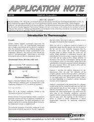
Effective Value<br />
The "effective" value <strong>of</strong> symmetrical periodic<br />
voltage (current) functions <strong>of</strong> time is based on the<br />
concept <strong>of</strong> "heating capability". Consider the test<br />
fixture shown in Figure 1.<br />
<strong>Voltage</strong><br />
Source<br />
Vx<br />
Figure 1<br />
Test Fixture<br />
Vessel<br />
Equilibrium<br />
Temperature<br />
Tx<br />
This vessel is insulated <strong>and</strong> filled with some stable<br />
liquid (transformer oil for example) capable <strong>of</strong><br />
reaching thermodynamic equilibrium. If a DC<br />
voltage Vx is applied to the vessel's internal heater,<br />
the liquid temperature will rise. Eventually, the<br />
electrical energy applied to this vessel will establish<br />
an equilibrium condition where energy input equals<br />
energy (heat) lost <strong>and</strong> the vessel liquid will arrive at<br />
an equilibrium temperature, Tx degrees.<br />
Next in this experimental scenario, replace the DC<br />
voltage source Vx with a time varying voltage which<br />
does not increase without bound. Eventually, in<br />
some time T final , thermal equilibrium will again be<br />
established. If this equilibrium condition establishes<br />
the same temperature Tx as reached before with the<br />
applied DC voltage Vx, then one can say that the<br />
"effective" value <strong>of</strong> this time varying function is Vx.<br />
Hence the definition <strong>of</strong> "effective value".
AN101 Dataforth Corporation Page 2 <strong>of</strong> 6<br />
Equation 2 illustrates this thermal equilibrium.<br />
2 2<br />
(( V ) / R) * T = z ( V( t) / R)<br />
dt Eqn 2<br />
Effective<br />
final<br />
T final<br />
0<br />
If V(t) is a periodic function <strong>of</strong> time with a cycle<br />
period <strong>of</strong> Tp, <strong>and</strong> T final is an integer "n" times the<br />
period (n*Tp) then the integral over T final is simply<br />
n times the integral over Tp. The results <strong>of</strong> these<br />
substitutions are shown in Equation 3.<br />
z<br />
Tp<br />
2<br />
V Effective<br />
= (/ 1Tp)* Vt () dt, <strong>RMS</strong> Eqn 3<br />
0<br />
Equation 3 illustrates that the effective equivalent<br />
heating capacity <strong>of</strong> a bounded periodic voltage<br />
(current) function can be determined over just one<br />
cycle. This equation is recognized as the old familiar<br />
form <strong>of</strong> "square Root <strong>of</strong> the Mean (average)<br />
Squared"; hence, the name, "<strong>RMS</strong>".<br />
Examples <strong>of</strong> Using the "<strong>RMS</strong>" Equation<br />
The following results can be shown by direct<br />
application <strong>of</strong> Eqn 3.<br />
Note: These examples illustrate that the shape <strong>of</strong> a<br />
periodic function can determine its <strong>RMS</strong> value. The<br />
peak (crest) <strong>of</strong> a voltage (current) function <strong>of</strong> time<br />
divided by 2 is <strong>of</strong>ten mistakenly used to calculate<br />
the <strong>RMS</strong> value. This technique can result in errors<br />
<strong>and</strong> clearly should be avoided.<br />
Effective (<strong>RMS</strong>) <strong>Values</strong> <strong>of</strong> Complex Functions<br />
An extremely useful fact in determining <strong>RMS</strong> values<br />
is that any well behaved bounded periodic function<br />
<strong>of</strong> time can be expressed as an average value plus a<br />
sum <strong>of</strong> sinusoids (Fourier's Theorem), for example;<br />
V(t) = Ao + ∑ [ An*Cos(nω o t) +Bn*Sin(nω o t) ]<br />
Summed over all "n" values Eqn 4<br />
Where ω o is the radian frequency <strong>of</strong> V(t) <strong>and</strong> An,<br />
Bn, Ao are Fourier Amplitude Coefficients.<br />
When this series is substituted in the integral<br />
expression Equation 2 for <strong>RMS</strong>, one obtains the<br />
following;<br />
Vrms= { ∑ [( A ) + ( A ) / 2+<br />
( B ) / 2 ]}<br />
0 2 n<br />
2 n<br />
2<br />
1. Sinusoidal function, peak <strong>of</strong> Vp<br />
V<strong>RMS</strong> = Vp ÷<br />
2 ; Vp*0.707<br />
Summed over all "n" values Eqn 5<br />
2<br />
2<br />
Note: ( A n ) / 2 <strong>and</strong> ( B n<br />
) / 2 are the squares <strong>of</strong><br />
th<br />
<strong>RMS</strong> values for each n Sin <strong>and</strong> Cosine component.<br />
2. Symmetrical Periodic Pulse Wave, peak <strong>of</strong> Vp The important conclusion is;<br />
V<strong>RMS</strong> = Vp (Symmetric Square Wave)<br />
3. Non-symmetrical Periodic Pulse Wave, all<br />
positive peaks <strong>of</strong> Vp, with duty cycle D<br />
V<strong>RMS</strong> = Vp *<br />
D<br />
D ≡ Td/Tp, Pulse duration Td ÷ Period Tp<br />
4. Symmetrical Periodic Triangle Wave, peak Vp<br />
V<strong>RMS</strong> = Vp ÷<br />
3 ; Vp * 0.5774 (Saw-Tooth)<br />
5. Full wave Rectified Sinusoid, peak Vp<br />
A bounded periodic function <strong>of</strong> time has a <strong>RMS</strong><br />
value equal to the square root <strong>of</strong> the sum <strong>of</strong> the<br />
square <strong>of</strong> each individual component's <strong>RMS</strong> value.<br />
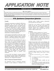
Practical Considerations<br />
Figure 2 illustrates composite curves formed by<br />
adding two sinusoids, one at 60 Hz <strong>and</strong> one at<br />
180Hz. Curve 1 is for zero phase difference <strong>and</strong><br />
Curve 2 is for a 90-degree phase difference.<br />
Specifically;<br />
V<strong>RMS</strong> = Vp ÷ 2 ; Vp * 0.707 Curve 1 V(t) = 170*Sin(377*t) +50*Sin(1131*t)<br />
6. Half Wave Rectified Sinusoid, peak Vp<br />
Curve 2 V(t) = 170*Sin(377*t) +50*Cos(1131*t)<br />
V<strong>RMS</strong> = Vp ÷2; Vp * 0.5<br />
Note: Composite curve shape is determined by<br />
phase <strong>and</strong> frequency harmonics.
AN101 Dataforth Corporation Page 3 <strong>of</strong> 6<br />
(1) 170*Sin 60Hz +50*Sin 180Hz Volts<br />
200<br />
100.0<br />
0<br />
-100.0<br />
-200<br />
(2) 170*Sin 60Hz +50*Cos 180Hz Volts<br />
200<br />
100.0<br />
0<br />
-100.0<br />
-200<br />
17.0M 21.0M 25.0M 29.0M 33.0M<br />
TIME in Secs<br />
Figure 2<br />
Fundamental with Third Harmonic Added<br />
Curve 2 170*Sin(377*t) +50*Cos(1131*t)<br />
Curve 1 170*Sin(377*t) +50*Sin(1131*t)<br />
Industrial sinusoidal functions <strong>of</strong> voltage (current)<br />
<strong>of</strong>ten contain harmonics that impact wave shape <strong>and</strong><br />
peak (crest) values. For example, Curve 2 is typical<br />
<strong>of</strong> the magnetizing currents in 60 Hz transformers<br />
<strong>and</strong> motors. Inexpensive <strong>RMS</strong> reading devices <strong>of</strong>ten<br />
use a rectifier circuits that capture the peak value,<br />
which is then scaled by 0.707 <strong>and</strong> displayed as<br />
<strong>RMS</strong>. Clearly this technique can give incorrect <strong>RMS</strong><br />
readings. In this example, using Vpeak ÷ 2<br />
clearly gives incorrect values.<br />
1<br />
2<br />
measurement device for a saw-tooth function needed<br />
to achieve an <strong>RMS</strong> reading within 0.3% error<br />
requires a b<strong>and</strong>width, which includes the twentyfifth<br />
(25) harmonic <strong>and</strong> the resolution to read 10 mV<br />
levels.<br />
Assume, for illustration purposes, that an AC ripple<br />
on the DC output <strong>of</strong> a rectifier can be approximated<br />
by a saw-tooth function. Table 1 illustrates that to<br />
measure within a 0.3% error the AC <strong>RMS</strong> ripple on<br />
the DC output <strong>of</strong> a 20 kHz rectifier the measurement<br />
device must have a b<strong>and</strong>width in excess <strong>of</strong> 500 kHz<br />
<strong>and</strong> a resolution to read voltage levels down by 40<br />
dB (100 microvolts for a peak 10 mV ripple). This<br />
example clearly illustrates that signal shape, together<br />
with the measurement b<strong>and</strong>width <strong>and</strong> resolution are<br />
extremely important in determining the accuracy <strong>of</strong><br />
measuring true <strong>RMS</strong>.<br />
Any "true <strong>RMS</strong>" measurement device must be<br />
capable <strong>of</strong> accurately implement Eqn 3. The subtlety<br />
in this statement is that electronically implementing<br />
Eqn 3, requires a device to have a very large<br />
b<strong>and</strong>width <strong>and</strong> be able to resolve small magnitudes.<br />
Crest Factor<br />
Another figure <strong>of</strong> merit <strong>of</strong>ten used to characterize a<br />
periodic time function <strong>of</strong> voltage (current) is the<br />
Crest Factor (CF). The Crest Factor for a specific<br />
waveform is defined as the peak value divided by<br />
the <strong>RMS</strong> value. Specifically,<br />
CF = V peak / V <strong>RMS</strong> Eqn 6<br />
Curve 1: 203*0.707 = 144 volts, not true <strong>RMS</strong><br />
Curve 2: 155*0.707 = 110 volts, not true <strong>RMS</strong><br />
Examples: (from page 2)<br />
The correct <strong>RMS</strong> value for both <strong>of</strong> these composite<br />
1. Pure Sinusoid, CF = 2<br />
sinusoidal functions is; 2. Symmetrical Periodic Pulses, CF = 1<br />
[ (170) 2 /2 + (50) 2 /2 ] 1/2 = 125.3 volts <strong>RMS</strong> 3. Non-symmetrical Periodic Pulses with duty<br />
Table 1 illustrates two examples <strong>of</strong> <strong>RMS</strong> cycle D, CF = 1÷ D<br />
calculations by using individual Fourier coefficients<br />
<strong>and</strong> Eqn 5. Example one is a full wave rectified 1-<br />
volt peak sinusoid. Note that for a full wave rectified<br />
function the measurement device needed to achieve<br />
Example; If D = 5%, CF = 4.47<br />
4. Symmetrical Periodic Triangle, CF = 3<br />
a <strong>RMS</strong> reading within 0.01% error requires a 5. Full wave Rectified Sinusoid, CF = 2<br />
b<strong>and</strong>width, which includes the fifth (5) harmonic<br />
<strong>and</strong> the resolution to read 10 mV levels.<br />
The other example illustrated in Table 1 is a sawtooth<br />
6. Half Wave Rectified Sinusoid, CF = 2<br />
From Figure 2;<br />
1-volt peak function. For this example, the Curve 1, CF =<br />
1.62<br />
Curve 2, CF = 1.24
AN101 Dataforth Corporation Page 4 <strong>of</strong> 6<br />
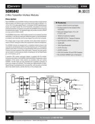
DATAFORTH <strong>RMS</strong> MEASUREMENT DEVICES<br />
True <strong>RMS</strong> measurements require instrumentation devices that accurately implement Eqn 3, "the" <strong>RMS</strong><br />
equation. These devices must have both wide b<strong>and</strong>widths <strong>and</strong> good low level resolution to support high Crest<br />
Factors. Dataforth has developed two products that satisfy these requirements; the SCM5B33 <strong>and</strong> DSCA33<br />
True <strong>RMS</strong> Input modules. Both these products provide a 1500Vrms isolation barrier between input <strong>and</strong> output.<br />
The SCM5B33 is a plug-in-panel module, <strong>and</strong> the DSCA33 is a DIN rail mount device. Each provide a single<br />
channel <strong>of</strong> AC input that is converted to its True <strong>RMS</strong> DC value, filtered, isolated, amplified, <strong>and</strong> converted to<br />
st<strong>and</strong>ard process voltage or current output.<br />
SCM5B33 ISOLATED TRUE <strong>RMS</strong><br />
INPUT MODULE, PLUG-IN-PANEL<br />
MOUNT<br />
FEATURES<br />
• INTERFACES <strong>RMS</strong> VOLTAGE (0 - 300V) OR<br />
<strong>RMS</strong> CURRENT (0 - 5A)<br />
• DESIGNED FOR STANDARD OPERATION<br />
WITH FREQUENCIES OF 45HZ TO 1000HZ<br />
(EXTENDED RANGE TO 20Khz)<br />
• COMPATIBLE WITH STANDARD CURRENT<br />
AND POTENTIAL TRANSFORMERS<br />
• INDUSTRY STANDARD OUTPUTS OF EITHER<br />
0-1MA, 0-20ma, 4-20 MA, 0-5V OR 0-10VDC<br />
• ±0.25% FACTORY CALIBRATED ACCURACY<br />
(ACCURACY CLASS 0.2)<br />
• 1500 V<strong>RMS</strong> CONTINUOUS TRANSFORMER<br />
BASED ISOLATION<br />
• INPUT OVERLOAD PROTECTED TO 480V MAX<br />
(PEAK AC & DC) OR 10A <strong>RMS</strong> CONTINUOUS<br />
• ANSI/IEEE C37.90.1-1989 TRANSIENT<br />
PROTECTION<br />
CSA AND FM APPROVALS PENDING<br />
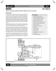
DESCRIPTION<br />
Each SCM5B33 True <strong>RMS</strong> input module provides a<br />
single channel <strong>of</strong> AC input which is converted to its True<br />
<strong>RMS</strong> dc value, filtered, isolated, amplified, <strong>and</strong> converted<br />
to a st<strong>and</strong>ard process voltage or current output (see<br />
diagram below).<br />
The SCM5B modules are designed with a completely<br />
isolated computer side circuit, which can be floated to<br />
±50V from Power Common, pin 16. This complete<br />
isolation means that no connection is required between<br />
I/O Common <strong>and</strong> Power Common for proper operation <strong>of</strong><br />
the output switch. If desired, the output switch can<br />
be turned on continuously by simply connecting pin 22,<br />
the Read-Enable pin to I/O Common, pin 19.<br />
The field voltage or current input signal is processed<br />
through a pre-amplifier <strong>and</strong> <strong>RMS</strong> converter on the field<br />
side <strong>of</strong> the isolation barrier. The converted dc signal is<br />
then chopped by a proprietary chopper circuit <strong>and</strong><br />
transferred across the transformer isolation barrier,<br />
suppressing transmission <strong>of</strong> common mode spikes <strong>and</strong><br />
surges. The computer side circuitry reconstructs filters<br />
<strong>and</strong> converts the signal to industry st<strong>and</strong>ard outputs.<br />
Modules are powered from +5VDC, ±5%.<br />
For current output models an external loop supply is<br />
required having a compliance voltage <strong>of</strong> 14 to 48VDC.<br />
Connection, with series load, is between Pin 20 (+) <strong>and</strong><br />
Pin 19 (-).
AN101 Dataforth Corporation Page 5 <strong>of</strong> 6<br />
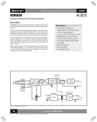
DSCA33 ISOLATED TRUE <strong>RMS</strong><br />
INPUT MODULE, DIN RAIL<br />
MOUNT<br />
FEATURES<br />
• INTERFACES <strong>RMS</strong> VOLTAGE (0 - 300V) OR<br />
<strong>RMS</strong> CURRENT (0 - 5A)<br />
• DESIGNED FOR STANDARD OPERATION<br />
WITH FREQUENCIES OF 45HZ TO 1000HZ<br />
(EXTENDED RANGE OPERATION TO 20kHZ)<br />
• COMPATABLE WITH STANDARD CURRENT<br />
AND POTENTIAL TRANSFORMERS<br />
• INDUSTRY STANDARD OUTPUTS OF EITHER<br />
0-1MA, 0-20MA, 4-20MA, 0-5V, OR 0-10VDC<br />
• ±0.25% FACTORY CALIBRATED ACCURACY<br />
(ACCURACY CLASS 0.2)<br />
• ±5% ADJUSTABLE ZERO AND SPAN<br />
1500 V<strong>RMS</strong> CONTINUOUS TRANSFORMER<br />
BASED ISOLATION<br />
• INPUT OVERLOAD PROTECTED TO 480V<br />
(PEAK AC & DC) OR 10A <strong>RMS</strong> CONTINUOUS<br />
• ANSI/IEEE C37.90.1-1989 TRANSIENT<br />
PROTECTION<br />
• MOUNTS ON STANDARD DIN RAIL<br />
• CSA AND FM APPROVALS PENDING<br />
DESCRIPTION<br />
Each DSCA33 True <strong>RMS</strong> input module provides a single<br />
channel <strong>of</strong> AC input which is converted to its True <strong>RMS</strong><br />
DC value, filtered, isolated, amplified, <strong>and</strong> converted to<br />
st<strong>and</strong>ard process voltage or current output (see diagram<br />
below).<br />
The field voltage or current input signal is processed<br />
through an AC coupled pre-amplifier <strong>and</strong> <strong>RMS</strong> converter<br />
on the field side <strong>of</strong> the isolation barrier. The converted<br />
DC signal is then filtered <strong>and</strong> chopped by a proprietary<br />
chopper circuit <strong>and</strong> transferred across the transformer<br />
isolation barrier, suppressing transmission <strong>of</strong> common<br />
mode spikes <strong>and</strong> surges.<br />
Module output is either voltage or current. For current<br />
output models a dedicated loop supply is provided at<br />
terminal 3 (+OUT) with loop return located at terminal 4<br />
(-OUT).<br />
Special input circuits provide protection against<br />
accidental connection <strong>of</strong> power-line voltages up to<br />
480VAC <strong>and</strong> against transient events as defined by<br />
ANSI/IEEE C37.90.1-1989. Protection circuits are also<br />
present on the signal output <strong>and</strong> power input terminals to<br />
guard against transient events <strong>and</strong> power reversal. Signal<br />
<strong>and</strong> power lines are secured to the module using<br />
pluggable terminal blocks.<br />
DSCA33 modules have excellent stability over time <strong>and</strong><br />
do not require recalibration, however, both zero <strong>and</strong> span<br />
settings are adjustable to accommodate situations where<br />
fine-tuning is desired. The adjustments are made using<br />
potentiometers located under the front panel label <strong>and</strong> are<br />
non-interactive for ease <strong>of</strong> use.
AN101 Dataforth Corporation Page 6 <strong>of</strong> 6<br />
Table 1<br />
<strong>RMS</strong> Calculated from Individual Fourier Coefficients<br />
Full-wave Rectified,1 Volt Peak<br />
Saw-Tooth Function,1 Volt Peak<br />
n<br />
An An (rms^2) Total rms % Error Bn Bn (rms^2) Total rms % Error<br />
0<br />
6.36620E-01 4.05285E-01 6.366198E-01 9.9684 5.00000E-01 2.500E-01 5.0000E-01 13.397<br />
1<br />
4.24413E-01 9.00633E-02 7.038096E-01 0.4663 3.18310E-01 5.066E-02 5.4833E-01 5.027<br />
2<br />
8.48826E-02 3.60253E-03 7.063643E-01 0.1050 1.59155E-01 1.267E-02 5.5976E-01 3.048<br />
3<br />
3.63783E-02 6.61689E-04 7.068325E-01 0.0388 1.06103E-01 5.629E-03 5.6476E-01 2.181<br />
4<br />
2.02102E-02 2.04225E-04 7.069770E-01 0.0184 7.95775E-02 3.166E-03 5.6756E-01 1.696<br />
5<br />
1.28610E-02 8.27027E-05 7.070355E-01 0.0101 6.36620E-02 2.026E-03 5.6934E-01 1.388<br />
6<br />
8.90377E-03 3.96386E-05 7.070635E-01 0.0061 5.30516E-02 1.407E-03 5.7057E-01 1.174<br />
7<br />
6.52943E-03 2.13168E-05 7.070786E-01 0.0040 4.54728E-02 1.034E-03 5.7148E-01 1.017<br />
8<br />
4.99310E-03 1.24655E-05 7.070874E-01 0.0027 3.97887E-02 7.916E-04 5.7217E-01 0.897<br />
9<br />
3.94192E-03 7.76936E-06 7.070929E-01 0.0020 3.53678E-02 6.254E-04 5.7272E-01 0.802<br />
10<br />
3.19108E-03 5.09148E-06 7.070965E-01 0.0015 3.18310E-02 5.066E-04 5.7316E-01 0.726<br />
11<br />
2.63611E-03 3.47453E-06 7.070989E-01 0.0011 2.89373E-02 4.187E-04 5.7352E-01 0.663<br />
12<br />
2.21433E-03 2.45163E-06 7.071007E-01 0.0009 2.65258E-02 3.518E-04 5.7383E-01 0.609<br />
13<br />
1.88628E-03 1.77903E-06 7.071019E-01 0.0007 2.44854E-02 2.998E-04 5.7409E-01 0.564<br />
14<br />
1.62610E-03 1.32211E-06 7.071029E-01 0.0006 2.27364E-02 2.585E-04 5.7432E-01 0.525<br />
15<br />
1.41628E-03 1.00293E-06 7.071036E-01 0.0005 2.12207E-02 2.252E-04 5.7451E-01 0.491<br />
16<br />
1.24461E-03 7.74531E-07 7.071041E-01 0.0004 1.98944E-02 1.979E-04 5.7469E-01 0.461<br />
17<br />
* * * * 1.87241E-02 1.753E-04 5.7484E-01 0.435<br />
18<br />
* * * * 1.76839E-02 1.564E-04 5.7497E-01 0.412<br />
19<br />
* * * * 1.67532E-02 1.403E-04 5.7510E-01 0.390<br />
20<br />
* * * * 1.59155E-02 1.267E-04 5.7521E-01 0.371<br />
21<br />
* * * * 1.51576E-02 1.149E-04 5.7531E-01 0.354<br />
22<br />
* * * * 1.44686E-02 1.047E-04 5.7540E-01 0.338<br />
23<br />
* * * * 1.38396E-02 9.577E-05 5.7548E-01 0.324<br />
24<br />
* * * * 1.32629E-02 8.795E-05 5.7556E-01 0.311<br />
25<br />
* * * * 1.27324E-02 8.106E-05 5.7563E-01 0.298<br />
Exact <strong>RMS</strong> 7.071068E-01 0 Exact <strong>RMS</strong> 5.7735E-01 0