High order splitting methods for analytic semigroups exist
High order splitting methods for analytic semigroups exist
High order splitting methods for analytic semigroups exist

Create successful ePaper yourself
Turn your PDF publications into a flip-book with our unique Google optimized e-Paper software.
BIT manuscript No.<br />
(will be inserted by the editor)<br />
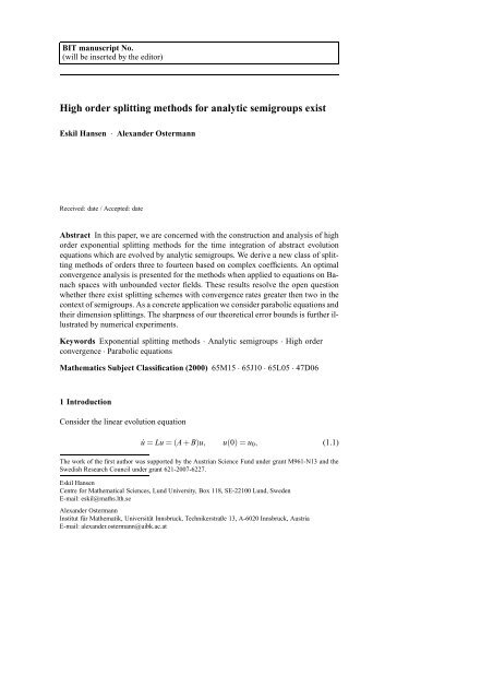
<strong>High</strong> <strong>order</strong> <strong>splitting</strong> <strong>methods</strong> <strong>for</strong> <strong>analytic</strong> <strong>semigroups</strong> <strong>exist</strong><br />
Eskil Hansen · Alexander Ostermann<br />
Received: date / Accepted: date<br />
Abstract In this paper, we are concerned with the construction and analysis of high<br />
<strong>order</strong> exponential <strong>splitting</strong> <strong>methods</strong> <strong>for</strong> the time integration of abstract evolution<br />
equations which are evolved by <strong>analytic</strong> <strong>semigroups</strong>. We derive a new class of <strong>splitting</strong><br />
<strong>methods</strong> of <strong>order</strong>s three to fourteen based on complex coefficients. An optimal<br />
convergence analysis is presented <strong>for</strong> the <strong>methods</strong> when applied to equations on Banach<br />
spaces with unbounded vector fields. These results resolve the open question<br />
whether there <strong>exist</strong> <strong>splitting</strong> schemes with convergence rates greater then two in the<br />
context of <strong>semigroups</strong>. As a concrete application we consider parabolic equations and<br />
their dimension <strong>splitting</strong>s. The sharpness of our theoretical error bounds is further illustrated<br />
by numerical experiments.<br />
Keywords Exponential <strong>splitting</strong> <strong>methods</strong> · Analytic <strong>semigroups</strong> · <strong>High</strong> <strong>order</strong><br />
convergence · Parabolic equations<br />
Mathematics Subject Classification (2000) 65M15 · 65J10 · 65L05 · 47D06<br />
1 Introduction<br />
Consider the linear evolution equation<br />
˙u = Lu = (A+B)u, u(0) = u 0 , (1.1)<br />
The work of the first author was supported by the Austrian Science Fund under grant M961-N13 and the<br />
Swedish Research Council under grant 621-2007-6227.<br />
Eskil Hansen<br />
Centre <strong>for</strong> Mathematical Sciences, Lund University, Box 118, SE-22100 Lund, Sweden<br />
E-mail: eskil@maths.lth.se<br />
Alexander Ostermann<br />
Institut für Mathematik, Universität Innsbruck, Technikerstraße 13, A-6020 Innsbruck, Austria<br />
E-mail: alexander.ostermann@uibk.ac.at
2 Eskil Hansen, Alexander Ostermann<br />
where the unbounded operators L, A and B generate the <strong>semigroups</strong> e tL , e tA and e tB ,<br />
respectively. Equations of this <strong>for</strong>m are, <strong>for</strong> example, found in the context of parabolic<br />
problems. A commonly used approach when approximating the solution u(t) = e tL u 0<br />
is to employ an s-stage exponential <strong>splitting</strong> scheme, i.e., u(nh) ≈ S n h u 0 with<br />
S h = e γ shA e δ shB ...e γ 1hA e δ 1hB . (1.2)<br />
The main advantage of these integrators is that they only rely on computations involving<br />
the partial flows e tA and e tB , which may tremendously improve the efficiency<br />
when compared to integrators based on approximating e tL u 0 directly. Contemporary<br />
surveys addressing the usage of exponential <strong>splitting</strong> <strong>methods</strong> can be found in [6,10,<br />
11].<br />
The coefficients γ j and δ j in (1.2) are chosen in such a way that the method has<br />
classical <strong>order</strong> p, which is achieved by <strong>for</strong>mally expanding S h and e hL into Taylor<br />
series in h and comparing the terms in the expansion up to <strong>order</strong> p. Our theory, presented<br />
in the paper [7], then yields that the <strong>splitting</strong> method will retain its classical<br />
<strong>order</strong> in the present context of unbounded operators.<br />
It has been a longstanding belief within the numerical analysis community that<br />
it is only possible to apply exponential <strong>splitting</strong> <strong>methods</strong> of at most <strong>order</strong> p = 2 to<br />
evolution equations which are evolved by <strong>semigroups</strong>. This statement is motivated<br />
by the fact that <strong>splitting</strong> schemes with real coefficients γ j and δ j necessarily have at<br />
least one negative coefficient whenever p ≥ 3; see [2]. Hence, one can not make use<br />
of such schemes here, as the <strong>semigroups</strong> are not well defined <strong>for</strong> negative times t.<br />
As an illustration, consider the somewhat trivial example of the semigroup e t∆ obtained<br />
when solving the heat equation ˙u = ∆u on the unit interval with homogeneous<br />
Dirichlet boundary conditions. Here, the kth Fourier coefficient of e t∆ u 0 is of the <strong>for</strong>m<br />
c k e −(kπ)2t and it is clear that the semigroup is in general not well defined <strong>for</strong> t < 0 in,<br />
e.g., L 2 (0,1).<br />
What is commonly overlooked is that the statement regarding the <strong>order</strong> p = 2<br />
barrier <strong>for</strong> <strong>splitting</strong> schemes only holds true <strong>for</strong> real coefficients γ j and δ j , whereas<br />
the <strong>order</strong> conditions yield plenty of schemes of <strong>order</strong> p ≥ 3 with complex coefficients<br />
in the right half plane of C. Some examples of such <strong>splitting</strong> schemes are given in the<br />
papers [1,4,16]. The question is now if one can make sense of the <strong>semigroups</strong> in this<br />
complex valued setting. If we return to the example of the heat equation on the unit<br />
interval, it is straight<strong>for</strong>ward to extend e t∆ to complex times t ∈ {z ∈ C : Re(z) ≥ 0} by<br />
using Parseval’s equality. In fact, when treating parabolic equations one can always<br />
extend the related semigroup into a sector in the right half plane of C, which leads to<br />
the theory of <strong>analytic</strong> <strong>semigroups</strong>. Thus, the aim of this paper is to derive and analyze<br />
a new broad class of complex <strong>splitting</strong> schemes, of <strong>order</strong> p ≥ 3 and with coefficients<br />
having positive real parts (and small arguments), which can be applied to (1.1).<br />
The paper is organized as follows: We start off in Section 2 by systematically deriving<br />
<strong>splitting</strong> schemes with complex coefficients and of high classical <strong>order</strong>. Thereafter,<br />
in Section 3, we present the needed framework of <strong>analytic</strong> <strong>semigroups</strong> and<br />
recapitulate the central convergence result. A concrete application of the abstract theory<br />
is given in Section 4, where we consider the dimension <strong>splitting</strong> of parabolic<br />
problems. Finally, the theoretical results are illustrated in Section 5, by a wide range<br />
of numerical experiments.
<strong>High</strong> <strong>order</strong> <strong>splitting</strong> <strong>methods</strong> <strong>for</strong> <strong>analytic</strong> <strong>semigroups</strong> <strong>exist</strong> 3<br />
2 Derivation of high <strong>order</strong> <strong>splitting</strong> schemes with complex coefficients<br />
Our first step is to derive <strong>splitting</strong> schemes (1.2) of classical <strong>order</strong> p ≥ 3 with coefficients<br />
γ j and δ j in the right half plane of C. There are (at least) two basic strategies<br />
to achieve this, either by deriving the schemes from scratch via <strong>order</strong> conditions, or<br />
by constructing them via the composition of lower <strong>order</strong> <strong>splitting</strong>s. After the submission<br />
of the paper, it has come to our attention that the latter approach has also<br />
been proposed in the preprint [3]. As a convention, named <strong>splitting</strong>s will be denoted<br />
hence<strong>for</strong>th by capital Greek letters, Φ h , Ψ h , etc.<br />
2.1 Deriving schemes from scratch<br />
It is possible to obtain <strong>order</strong> conditions <strong>for</strong> an exponential <strong>splitting</strong> scheme by employing<br />
the so called Baker–Campbell–Hausdorff <strong>for</strong>mula; see [6, Section III.5]. For<br />
example, the <strong>order</strong> conditions obtained <strong>for</strong> an s-stage exponential <strong>splitting</strong> of <strong>order</strong><br />
p = 3 are<br />
c 1 1,s = c 1 2,s = 1 and c 2 1,s = c 3 1,s = c3 2,s = 0, (2.1)<br />
where the terms c k l,s<br />
are given by the recurrence relations<br />
c 1 1, j = c1 1, j−1 + δ j, c 1 2, j = c1 2, j−1 + γ j,<br />
c 2 1, j = c 2 1, j−1 + δ j γ j + c 1 1, j−1γ j − c 1 2, j−1δ j ,<br />
c 3 1, j = c3 1, j−1 + δ 2 j γ j + 2c 1 1, j−1δ j γ j − 3c 2 1, j−1δ j<br />
+(c 1 1, j−1 )2 γ j − c 1 1, j−1 c1 2, j−1δ j + c 1 2, j−1δ 2 j ,<br />
c 3 2, j = c3 2, j−1 + δ jγ 2 j − 4c1 2, j−1δ j γ j + 3c 2 1, j−1γ j<br />
+(c 1 2, j−1) 2 δ j − c 1 1, j−1c 1 2, j−1γ j + c 1 1, j−1γ 2 j ,<br />
<strong>for</strong> j ≥ 1, and c k l,0<br />
= 0 <strong>for</strong> all values of k and l. The derivation can be found in<br />
connection with the proof of [6, Theorem III.5.6]. For a solution of (2.1), its complex<br />
conjugate is again a solution. This follows from the fact that the <strong>order</strong> conditions are<br />
real polynomials. There<strong>for</strong>e, we will determine solutions up to conjugation only.<br />
We next discuss how the <strong>order</strong> conditions (2.1) can be solved with a small number<br />
of stages. For s = 3, the <strong>order</strong> conditions consist of five polynomial equations with<br />
six unknowns γ 1 , γ 2 , γ 3 , δ 1 , δ 2 , and δ 3 . Generically, a one parameter family solutions<br />
<strong>exist</strong>s. For our purpose, it is essential that all method coefficients have positive real<br />
parts.<br />
Taking δ 2 = χ as free parameter, the <strong>order</strong> conditions are easily solved in the<br />
following way. With the help of the conditions c 1 1,s = c1 2,s = 1, we express δ 1 by δ 3<br />
and χ, as well as γ 1 by γ 2 and γ 3 . We insert these relations into c 2 1,s<br />
= 0 and solve <strong>for</strong><br />
γ 2 . There is a unique solution <strong>for</strong> χ ≠ 0. Next, we insert the so far computed quantities
4 Eskil Hansen, Alexander Ostermann<br />
0.7<br />
0.6<br />
0.5<br />
Re (γ 1<br />
) = Re (γ 2<br />
)<br />
Re (γ 3<br />
)<br />
Re (δ 1<br />
)<br />
Re (δ 2<br />
)<br />
Re (δ ) 3<br />
0.8<br />
0.6<br />
0.4<br />
Im (γ 1<br />
)<br />
Im (γ 2<br />
)<br />
Im (γ 3<br />
) = Im (δ 2<br />
)<br />
Im (δ 1<br />
)<br />
Im (δ 3<br />
)<br />
Real part<br />
0.4<br />
0.3<br />
Imaginary part<br />
0.2<br />
0<br />
−0.2<br />
0.2<br />
−0.4<br />
0.1<br />
−0.6<br />
0<br />
0 0.1 0.2 0.3 0.4 0.5<br />
χ<br />
−0.8<br />
0 0.1 0.2 0.3 0.4 0.5<br />
χ<br />
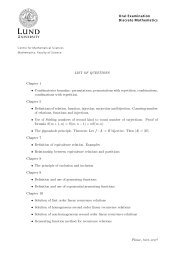
Fig. 2.1 The figures display the real (left) and imaginary (right) parts of the parameter dependent coefficients<br />
γ j and δ j , which determine the third <strong>order</strong> exponential <strong>splitting</strong> family Ψ h (χ).<br />
into c 3 1,s = 0 and solve <strong>for</strong> γ 3. Again, we get a unique solution <strong>for</strong> χ ≠ 0 and χ ≠ 3/4.<br />
The condition c 3 2,s = 0 then becomes a quadratic equation in δ 3 with the solutions<br />
δ 3 = 12 − 27χ + 12χ 2 ±<br />
√3χ ( 48χ 3 − 72χ 2 + 39χ − 8 )<br />
. (2.2)<br />
18 − 24χ<br />
Inserting this back gives the sought after family of solutions. For real χ ≥ 0, the<br />
resulting one parameter family of coefficients is displayed in Figure 2.1. The critical<br />
coefficient turns out to be<br />
γ 3 = 1 − 2χ<br />
4 − 6χ .<br />
To guarantee its admissability, we restrict our attention to the interval 0 < χ ≤ 1/2.<br />
For these values of χ the expression under the square root in (2.2) is negative and we<br />
thus get a unique solution (up to complex conjugation).<br />
Theorem 2.1 For 0 < χ ≤ 1/2, let the coefficients γ 1 , γ 2 , γ 3 , δ 1 , δ 2 , and δ 3 be defined<br />
by the above procedure. The exponential <strong>splitting</strong> schemes<br />
Ψ h (χ) = e γ 3(χ)hA e δ 3(χ)hB e γ 2(χ)hA e δ 2(χ)hB e γ 1(χ)hA e δ 1(χ)hB<br />
are then all of classical <strong>order</strong> p = 3.<br />
For some choices of χ the coefficients of Ψ h (χ) have a quite simple <strong>for</strong>m. A few<br />
examples are χ = 1/10, where the coefficients are<br />
γ 1 = 13<br />
34 − i √<br />
3579<br />
102 , δ 1 = 77<br />
260 − i √<br />
3579<br />
780 ,<br />
γ 2 = 13<br />
34 + i √<br />
3579<br />
102 , δ 2 = 1 10 ,<br />
γ 3 = 4<br />
17 , δ 3 = 157<br />
260 + i √<br />
3579<br />
780 ,<br />
⊓⊔
<strong>High</strong> <strong>order</strong> <strong>splitting</strong> <strong>methods</strong> <strong>for</strong> <strong>analytic</strong> <strong>semigroups</strong> <strong>exist</strong> 5<br />
and the choice χ = 1/3, which yields<br />
γ 1 = 5<br />
12 + i √<br />
11<br />
12 , δ 1 = 7<br />
30 + i √<br />
11<br />
30 ,<br />
γ 2 = 5<br />
12 − i √<br />
11<br />
12 , δ 2 = 1 3 ,<br />
γ 3 = 1 6 , δ 3 = 13<br />
30 − i √<br />
11<br />
30 .<br />
A particular case is obtained <strong>for</strong> χ = 1/2, where<br />
and the resulting scheme<br />
( 14<br />
−i<br />
Ψ h (1/2) = e<br />
γ 1 = 1 2 + i √<br />
3<br />
6 , δ 1 = 1 4 + i √<br />
3<br />
12 ,<br />
γ 2 = 1 2 − i √<br />
3<br />
6 , δ 2 = 1 2 ,<br />
γ 3 = 0, δ 3 = 1 4 − i √<br />
3<br />
12 ,<br />
√<br />
3<br />
12<br />
) ( √ )<br />
√<br />
hB 12<br />
−i 3<br />
e<br />
6 hA 1<br />
e hB 12<br />
+i 3<br />
2 e(<br />
( √<br />
6<br />
)hA 14<br />
+i 3<br />
e<br />
12<br />
)<br />
hB<br />
(2.3)<br />
only requires, in average, the evaluation of four semigroup actions instead of the<br />
normal six, see also [16, eq. (23)] and [14].<br />
Of course, the parameter χ can also be chosen complex. Even so, we will omit<br />
a further investigation since the derived family Ψ h (χ) already includes schemes with<br />
coefficients possessing fairly small arguments.<br />
2.2 Deriving schemes via compositions<br />
A second approach is to identify the <strong>splitting</strong> scheme as a composition method, and<br />
then to use the following result; see [6, Theorem II.4.1 and Section II.5].<br />
Lemma 2.1 Let S h be a one step method of classical <strong>order</strong> q. If<br />
σ 1 +...+ σ m = 1 and σ q+1<br />
1<br />
+...+ σ q+1<br />
m = 0, (2.4)<br />
then the composition method S σm h ...S σ1 h is at least of classical <strong>order</strong> q+1.<br />
⊓⊔<br />
Using this argument iteratively allows us to create <strong>splitting</strong> schemes with increasing<br />
classical <strong>order</strong>s. In the framework of <strong>analytic</strong> <strong>semigroups</strong>, however, this construction<br />
does not yield expedient <strong>methods</strong> of arbitrary <strong>order</strong>s by default. This is due to<br />
the fact that the arguments of the coefficients are added together in each composition<br />
step, which in the end may result in coefficients with non-positive real parts.<br />
In conclusion, when using the strategy of composition to generate high <strong>order</strong><br />
schemes <strong>for</strong> <strong>analytic</strong> <strong>semigroups</strong>, it is vital to find solutions of (2.4) with small arguments<br />
argσ l <strong>for</strong> 1 ≤ l ≤ m.
6 Eskil Hansen, Alexander Ostermann<br />
Two term compositions<br />
We will first consider compositions with m = 2. As a concrete example, let us employ<br />
the Strang <strong>splitting</strong><br />
Φ h = e 1 2 hB e hA e 1 2 hB ,<br />
which has classical <strong>order</strong> p = 2, as our starting scheme S h . We then proceed by introducing<br />
the following chain of two term compositions<br />
Φ h (k,2) = Φ σk,2 h(k − 1,2)Φ σk,1 h(k − 1,2), k ≥ 1,<br />
where Φ h (0,2) = Φ h and the coefficients σ k,1 and σ k,2 are solutions of (2.4) <strong>for</strong> m = 2<br />
and q = k+1. By eliminating one of the two variables, system (2.4) reduces to<br />
σ q+1 +(1 − σ) q+1 = 0<br />
or<br />
( σ<br />
) q+1<br />
= −1. (2.5)<br />
1 − σ<br />
By taking the logarithms, we easily derive that all solutions of (2.5) are given by<br />
σ = 1 2 + i<br />
( )<br />
sin 2l+1<br />
q+1 π<br />
2+2cos( 2l+1<br />
q+1 π ) <strong>for</strong><br />
⎧<br />
⎨− q 2 ≤ l ≤ q 2 − 1<br />
⎩− q+1<br />
2<br />
≤ l ≤ q − 1<br />
2<br />
if q is even,<br />
if q is odd.<br />
Since the function<br />
sinx<br />
, −π < x < π,<br />
2+2cosx<br />
is monotonically increasing, we get coefficients with the smallest angles <strong>for</strong> l = 0.<br />
We there<strong>for</strong>e obtain the following schemes with <strong>order</strong>s ranging from three to six.<br />
Theorem 2.2 Let 1 ≤ k ≤ 4. Then the exponential <strong>splitting</strong> schemes Φ h (k,2) with<br />
σ k,1 = 1 2 + i sin ( π/(k+2) )<br />
2+2cos ( π/(k+2) ) and σ k,2 = σ k,1<br />
are of <strong>order</strong> p = k+2.<br />
⊓⊔<br />
Note that the above two term composition can not be made <strong>for</strong> k ≥ 5 in the framework<br />
of <strong>analytic</strong> <strong>semigroups</strong>, as the <strong>splitting</strong>s Φ h (k,2) then have coefficients γ j and/or<br />
δ j with negative real parts. Further note that the third <strong>order</strong> <strong>splitting</strong> Ψ(1/2), given<br />
in (2.3), coincides with Φ h (1,2).
<strong>High</strong> <strong>order</strong> <strong>splitting</strong> <strong>methods</strong> <strong>for</strong> <strong>analytic</strong> <strong>semigroups</strong> <strong>exist</strong> 7<br />
Symmetric three term compositions<br />
In <strong>order</strong> to obtain <strong>methods</strong> of higher <strong>order</strong>, we have to increase the number m of<br />
terms in the composition. If the composition is symmetric, i.e., if σ m−l+1 = σ l <strong>for</strong><br />
all l, then the <strong>order</strong> of the resulting <strong>splitting</strong> scheme is even. Hence, if we make a<br />
symmetric composition with a <strong>splitting</strong> S h of even <strong>order</strong> p, then the resulting scheme<br />
S σm h...S σ1 h obtains an <strong>order</strong> of p+2; see [6, Section II.3 and II.5]<br />
As a first step, we construct symmetric three term compositions. Starting from<br />
the Strang <strong>splitting</strong> Φ h (0,3) = Φ h , we consider the following chain of compositions<br />
Φ h (k,3) = Φ σk,1 h(k − 1,3)Φ σk,2 h(k − 1,3)Φ σk,1 h(k − 1,3), k ≥ 1,<br />
where the coefficients σ k,1 and σ k,2 are solutions of (2.4) <strong>for</strong> m = 3 and q = 2k. By<br />
eliminating σ k,2 we obtain the polynomial<br />
( σ<br />
) q+1<br />
2σ q+1 +(1 − 2σ) q+1 1<br />
= 0 or<br />
= −<br />
1 − 2σ 2 . (2.6)<br />
By once again taking the logarithms, we have that the solutions of minimal argument<br />
are<br />
e πi/(2k+1)<br />
σ k,1 =<br />
2 1/(2k+1) + 2e πi/(2k+1) and σ k,2 = 1 − 2σ k,1 . (2.7)<br />
This results in the schemes below, with the <strong>order</strong>s ranging from four to eight.<br />
Theorem 2.3 Let 1 ≤ k ≤ 3. Then the exponential <strong>splitting</strong> schemes Φ h (k,3) with<br />
coefficients given by (2.7) are of <strong>order</strong> p = 2k+2.<br />
⊓⊔<br />
For our purpose, the three term compositions are useless <strong>for</strong> k ≥ 4, as the <strong>splitting</strong>s<br />
Φ h (k,3) then have coefficients with negative real parts.<br />
Symmetric four term compositions<br />
To gain even higher <strong>order</strong> schemes, we conclude by constructing symmetric four term<br />
compositions. Starting again from the Strang <strong>splitting</strong> Φ h (0,4) = Φ h , we consider the<br />
compositions<br />
Φ h (k,4) = Φ σk,1 h(k − 1,4)Φ σk,2 h(k − 1,4)Φ σk,2 h(k − 1,4)Φ σk,1 h(k − 1,4), k ≥ 1,<br />
where the coefficients σ k,1 and σ k,2 are solutions of (2.4) <strong>for</strong> m = 4 and q = 2k. By<br />
eliminating σ k,2 we obtain the polynomial<br />
( ) q+1 (<br />
σ q+1 + 1 2σ<br />
) q+1<br />
2 − σ = 0 or = −1.<br />
1 − 2σ<br />
(2.8)<br />
The solutions with minimal arguments are then<br />
σ k,1 = 1 4 + i sin ( π/(2k+1) )<br />
4+4cos ( π/(2k+1) ) and σ k,2 = σ k,1 , (2.9)<br />
and we get the schemes below of <strong>order</strong>s ranging from four to fourteen.<br />
Theorem 2.4 Let 1 ≤ k ≤ 6. Then the exponential <strong>splitting</strong> schemes Φ h (k,4) with<br />
coefficients given by (2.9) are of <strong>order</strong> p = 2k+2.<br />
⊓⊔<br />
For k ≥ 7 the <strong>splitting</strong>s Φ h (k,4) have coefficients with negative real parts.
8 Eskil Hansen, Alexander Ostermann<br />
3 The framework of <strong>analytic</strong> <strong>semigroups</strong> and convergence results<br />
We next present the framework of unbounded operators which enables us to prove<br />
that any exponential <strong>splitting</strong> method of classical <strong>order</strong> p, and with appropriate complex<br />
coefficients, will retain its <strong>order</strong> when applied to (1.1).<br />
Hence<strong>for</strong>th, X will denote an arbitrary (complex) Banach space with norm ‖ · ‖,<br />
and the corresponding operator norm will also be referred to as ‖ · ‖. Furthermore, C<br />
will be a generic constant which assumes different values at different occurrences. In<br />
our analysis, an essential tool are compositions of the operators A and B that consist<br />
of exactly k factors. We will denote such terms generically by E k . For instance,<br />
E 3 ∈ {AAA,AAB,ABA,BAA,ABB,BAB,BBA,BBB}.<br />
To enable our analysis, we will assume the following.<br />
Assumption 3.1 The linear operators L, A and B, all generate <strong>analytic</strong> <strong>semigroups</strong><br />
on X defined in the sector Σ φ = {z ∈ C : |argz| < φ}, <strong>for</strong> a given angle φ ∈ (0,π/2].<br />
Furthermore, the operators A and B satisfy the additional bounds<br />
<strong>for</strong> some ω ≥ 0 and all z ∈ Σ φ .<br />
‖e zA ‖ ≤ e ω|z| and ‖e zB ‖ ≤ e ω|z|<br />
Assumption 3.2 All expressions of the <strong>for</strong>m E p+1 u(t) are uni<strong>for</strong>mly bounded on the<br />
interval [0,T], <strong>for</strong> some T > 0.<br />
See [5, Section II.4.a] or [13, Section 2.2.5] <strong>for</strong> an introduction to the theory of<br />
<strong>analytic</strong> <strong>semigroups</strong>. Under these assumptions it is possible to prove the following<br />
convergence results.<br />
Theorem 3.1 For the numerical solution of (1.1), consider an exponential <strong>splitting</strong><br />
method (1.2) of classical <strong>order</strong> p, with all its coefficients γ j and δ j in the sector<br />
Σ φ ⊂ C. If Assumptions 3.1 and 3.2 are valid, then<br />
∥ ( S n h − enhL) u 0<br />
∥ ∥ ≤ Ch p , 0 ≤ nh ≤ T,<br />
where the constant C can be chosen uni<strong>for</strong>mly on bounded time intervals and, in<br />
particular, independent of n and h.<br />
Proof In our paper [7], we prove Theorem 3.1 <strong>for</strong> C 0 <strong>semigroups</strong> and exponential<br />
<strong>splitting</strong> schemes with real coefficients γ j and δ j ; see [7, Theorem 2.3 and Section<br />
4.4]. The proof is of an algebraic nature and when one has introduced the concept<br />
of <strong>analytic</strong> <strong>semigroups</strong>, as done in Assumption 3.1, it can be extended to the current<br />
setting of complex coefficients without changing any of the used arguments. ⊓⊔<br />
As the discrete evolution operator S h is complex valued, the above approach cannot<br />
be used directly to study problems in real Banach spaces X. A remedy would be<br />
to complexify X in the usual way to X ⊕ iX with the norm<br />
‖u+iv‖ = max<br />
(‖αu − β v‖ 2 + ‖αv+β u‖ 2) 1/2<br />
<strong>for</strong> u,v ∈ X,<br />
α 2 +β 2 =1
<strong>High</strong> <strong>order</strong> <strong>splitting</strong> <strong>methods</strong> <strong>for</strong> <strong>analytic</strong> <strong>semigroups</strong> <strong>exist</strong> 9<br />
see [15, Sect. 6.5]. For real initial data, the imaginary part of the numerical solution<br />
will stay O(h p ) on bounded time intervals. This follows at once from Theorem 3.1.<br />
Another possibility, however, would be to restrict the numerical evolution after<br />
each time step to its real part. This is achieved by the projection operator<br />
P : X ⊕ iX → X : u+iv ↦→ u.<br />
As this projection satisfies ‖P‖ = 1, the modified flow<br />
Ŝ h = PS h : X → X (3.1)<br />
is power-bounded <strong>for</strong> 0 ≤ nh ≤ T . This follows at once from Assumption 3.1. The<br />
global error at time t = nh has the representation<br />
n<br />
(Ŝh − e nhL) n−1<br />
u 0 =<br />
∑<br />
j=0<br />
Ŝ<br />
n− j−1<br />
h<br />
(<br />
P S h − e hL) e jhL u 0 ,<br />
and can be bounded in the same way as be<strong>for</strong>e. We thus get the following corollary.<br />
Corollary 3.1 For the numerical solution of (1.1) on a real Banach space, consider<br />
the <strong>splitting</strong> method (3.1). If the assumptions of Theorem 3.1 are valid, then<br />
∥ ( Ŝ n h − enhL) u 0<br />
∥ ∥ ≤ Ch p , 0 ≤ nh ≤ T,<br />
where the constant C can be chosen uni<strong>for</strong>mly on bounded time intervals and, in<br />
particular, independent of n and h.<br />
⊓⊔<br />
Note that the extension to <strong>splitting</strong>s of more then two operators and variable step<br />
sizes presented in [7, Section 4] are also generalizable to the present context of complex<br />
coefficients.<br />
As a direct consequence of Theorem 3.1, the <strong>splitting</strong> schemes derived in Section<br />
2 retain their classical <strong>order</strong> when applied to problems satisfying Assumption 3.1<br />
with a sufficiently large angle φ, i.e,<br />
φ > ϕ := max ( |arg γ 1 |,...,|arg γ s |,|arg δ 1 |,...,|arg δ s | ) .<br />
Hence, when designing <strong>splitting</strong> schemes <strong>for</strong> evolution equations governed by <strong>semigroups</strong><br />
one should try to minimize the method angle ϕ, as this gives rise to more<br />
widely applicable schemes. The <strong>order</strong>s and angles <strong>for</strong> the <strong>methods</strong> derived in Section<br />
2 are presented in Tables 3.1 and 3.2.<br />
Table 3.1 The method angles ϕ of the third <strong>order</strong> schemes presented in Section 2.1.<br />
S h Ψ h (1/10) Ψ h (1/3) Ψ h (1/2)<br />
ϕ 56.90 ◦ 33.56 ◦ 30 ◦
10 Eskil Hansen, Alexander Ostermann<br />
Table 3.2 The method angles ϕ and <strong>order</strong>s p <strong>for</strong> the composition schemes derived in Section 2.2.<br />
S h Φ h (0,2) Φ h (1,2) Φ h (2,2) Φ h (3,2) Φ h (4,2)<br />
ϕ 0 ◦ 30 ◦ 52.50 ◦ 70.50 ◦ 85.50 ◦<br />
p 2 3 4 5 6<br />
S h Φ h (0,3) Φ h (1,3) Φ h (2,3) Φ h (3,3)<br />
ϕ 0 ◦ 37.47 ◦ 60.49 ◦ 77.11 ◦<br />
p 2 4 6 8<br />
S h Φ h (0,4) Φ h (1,4) Φ h (2,4) Φ h (3,4) Φ h (4,4) Φ h (5,4) Φ h (6,4)<br />
ϕ 0 ◦ 30 ◦ 48 ◦ 60.86 ◦ 70.86 ◦ 79.04 ◦ 85.96 ◦<br />
p 2 4 6 8 10 12 14<br />
4 Dimension <strong>splitting</strong> of parabolic problems<br />
In <strong>order</strong> to illustrate that Assumptions 3.1 and 3.2 are reasonable <strong>for</strong> parabolic equations<br />
and their dimension <strong>splitting</strong>s, we give the following example:<br />
Let Ω be a bounded domain in R d with a sufficiently regular boundary ∂Ω and<br />
set X = L 2 (Ω). Consider the dimension <strong>splitting</strong> of the elliptic operator L = A+B,<br />
where<br />
s<br />
d<br />
Au = ∑ D i (a i D i u) and Bu = ∑ D j (a j D j u),<br />
i=1<br />
j=s+1<br />
the functions a i ∈ C ∞ (Ω) are real and positive, and D i = ∂/∂x i . Furthermore, we<br />
impose homogenous Dirichlet conditions on ∂Ω.<br />
To validate Assumption 3.1, we first restrict our attention to the operator A. The<br />
operator can be cast into the framework of <strong>analytic</strong> <strong>semigroups</strong> on X by introducing<br />
the sesquilinear <strong>for</strong>m<br />
s (√<br />
b(u,v) = ai D i u, √ a i D i v ) ,<br />
∑<br />
i=1<br />
where (·,·) is the inner product on X. Next, define the Hilbert space V with inner<br />
product<br />
(u,v) V = λ(u,v)+b(u,v) (4.1)<br />
as the completion of C0 ∞ (Ω) with respect to the norm induced by (4.1). Here, λ is<br />
a given positive parameter. Note that this yields the following chain of imbeddings<br />
V ֒→ X ∼ = X ′ ֒→ V ′ , where X ′ denotes the dual space of X. With this construction it is<br />
possible to interpret A as an unbounded operator on X with domain<br />
D(A) = {u ∈ V : ∃ y ∈ X with (y,v) = −b(u,v) ∀v ∈ V}<br />
and Au = y <strong>for</strong> all u ∈ D(A). To establish the generating properties of A, we first<br />
observe that<br />
(Au,u) = −b(u,u) ≤ 0 <strong>for</strong> all u ∈ D(A). (4.2)
<strong>High</strong> <strong>order</strong> <strong>splitting</strong> <strong>methods</strong> <strong>for</strong> <strong>analytic</strong> <strong>semigroups</strong> <strong>exist</strong> 11<br />
Secondly, by the Riesz representation theorem, there <strong>exist</strong>s a unique u ∈ V <strong>for</strong> every<br />
y ∈ X and λ > 0 such that<br />
(u,v) V = λ(u,v)+b(u,v) = (y,v) <strong>for</strong> all v ∈ V.<br />
Hence, u ∈ D(A) and (λ I −A)u=y, which implies the range propertyR(λ I −A)=X<br />
<strong>for</strong> all λ > 0. In conclusion, the hypotheses of the Lumer–Phillips theorem are valid,<br />
and the operator A there<strong>for</strong>e generates a C 0 semigroup of contractions on X, i.e., e zA<br />
is well defined <strong>for</strong> z ∈ [0,∞).<br />
We will next extend the semigroup to a sector Σ φ = {z ∈ C : |argz| < φ}. To this<br />
end, note that the inequality (4.2) yields that the numerical range of A is contained in<br />
the interval (−∞,0], and the range condition R(λ I − A) = X gives that the resolvent<br />
set of A, ρ(A), contains the interval (0,∞). These properties together with [13, Theorem<br />
1.3.9] implies the inclusion Σ π ⊂ ρ(A) and, <strong>for</strong> every ε ∈ (0,π/2), the resolvent<br />
bound<br />
‖(λ I − A) −1 ‖ ≤ M ε<br />
|λ |<br />
<strong>for</strong> all λ ∈ Σ π−ε \{0}.<br />
This is the standard characterization of a generator of an <strong>analytic</strong> semigroup on X,<br />
defined in the sector Σ π/2 ; see [5, Theorem II.4.6] or [13, Theorem 2.5.2]. The <strong>analytic</strong><br />
semigroup e zA is also contractive, i.e., ‖e zA ‖ ≤ 1 <strong>for</strong> all z ∈ Σ π/2 . This can be<br />
seen by integrating the inequality<br />
d<br />
( d<br />
dt ‖etzA u‖ 2 = 2Re<br />
dt etzA u,e u)<br />
tzA = 2Re(z) ( Ae tzA u,e tzA u ) ≤ 0<br />
from 0 to 1 with respect to t.<br />
By merely changing the number of terms in the sesquilinear <strong>for</strong>m b(·,·) and<br />
renumbering the dimensions, we can do the same interpretation of the operators L<br />
and B, which validates Assumption 3.1 <strong>for</strong> φ = π/2. One can also use similar techniques<br />
to show that Assumption 3.1 is valid <strong>for</strong> the periodic problem, i.e., Ω is a<br />
d-dimensional torus T d , or if one imposes Neumann boundary conditions. The same<br />
holds <strong>for</strong> the degenerate case as well, where the functions a i vanish at the boundary<br />
∂Ω; see [8, Example 5.2] <strong>for</strong> more details.<br />
Assumption 3.2 is valid whenever<br />
D(L p+1 ) ⊆ D(E p+1 ), (4.3)<br />
as e tL : D(L p+1 ) → D(L p+1 ) <strong>for</strong> all times t ∈ [0,T]. The periodic setting yields<br />
that D(L p+1 ) = H 2(p+1) (T d ), and inclusion (4.3) is then trivially verified <strong>for</strong> all<br />
p ≥ 1. The same is true <strong>for</strong> the degenerate problem, but the situation becomes more<br />
delicate when boundary conditions are imposed. As a simple example, we consider<br />
the Dirichlet Laplacian L = ∆ over the unit square Ω = (0,1) 2 . Here,<br />
D(L p+1 ) = {u ∈ H 2(p+1) (Ω) ⊂ C 2p (Ω) : u = Lu = L 2 u = ...L p u = 0 on ∂Ω},
12 Eskil Hansen, Alexander Ostermann<br />
and Lu = (∂ 2 n + ∂ 2<br />
t )u almost everywhere on ∂Ω, where ∂ n and ∂ t denote the normal<br />
and tangential derivatives, respectively. If we start with p = 1, then<br />
u ∈ D(L 2 )<br />
⇒<br />
{ u = 0 ⇒ ∂<br />
2<br />
t u = 0 a.e. on ∂Ω<br />
Lu = 0 ⇒ ∂n 2u = Lu − ∂ t 2u<br />
= 0<br />
⇒ Au = Bu = 0 on ∂Ω.<br />
a.e. on ∂Ω<br />
Note that the almost everywhere part can be dropped as Au and Bu are both continuous<br />
on Ω. This implies the inclusion D(L 2 ) ⊆ D(E 2 ). Continuing to p = 2, gives the<br />
additional condition<br />
L 2 u = ( ∂n 4 + ∂n 2 ∂t 2 + ∂t 2 ∂n 2 + ∂t<br />
4 ) (<br />
u = ∂<br />
4<br />
n + 2∂t 2 ∂n 2 )u = 0<br />
a.e. on ∂Ω,<br />
but one knows nothing about, <strong>for</strong> example, ∂n 4 u alone which is needed to validate<br />
that D(L 3 ) is a subset of D(A 3 )∩D(B 3 ). In conclusion, D(L p+1 ) can not be expected<br />
to be a subset of D(E p+1 ), <strong>for</strong> p ≥ 2, when one considers boundary conditions in<br />
general.<br />
5 Numerical experiments and implementation<br />
As a final step, we will demonstrate the per<strong>for</strong>mance of the derived <strong>splitting</strong> schemes.<br />
To this end, consider the evolution equation (1.1) with<br />
in the four cases below.<br />
Lu = (A+B)u = D 1 (aD 1 u)+D 2 (aD 2 u),<br />
[PER] The periodic case, where we set Ω = T 2 , with coordinates (x 1 ,x 2 ) ∈ [0,1) 2 ,<br />
a(x 1 ,x 2 ) = sin(2πx 1 )sin(2πx 2 )+2 and u 0 (x 1 ,x 2 ) = sin(2πx 1 )sin(2πx 2 ).<br />
[DEG] The degenerate case, i.e., a vanishes on ∂Ω. Here, Ω = (0,1) 2 ,<br />
a(x 1 ,x 2 ) = 16x 1 (1 − x 1 )x 2 (1 − x 2 ) and u 0 (x 1 ,x 2 ) = sin(3πx 1 )cos(3πx 2 ).<br />
[DIR] The case of homogenous Dirichlet boundary conditions, <strong>for</strong> which Ω = (0,1) 2 ,<br />
a(x 1 ,x 2 ) = 16x 1 (1 − x 1 )x 2 (1 − x 2 )+1 and u 0 (x 1 ,x 2 ) = ce − 1<br />
x 1 (1−x 1 ) − 1<br />
x 2 (1−x 2) ,<br />
where c is chosen such that ‖u 0 ‖ L ∞ (Ω) = 1.<br />
[NEU] The case of homogenous Neumann boundary conditions, where we use the<br />
same Ω, a and u 0 as <strong>for</strong> DIR.
<strong>High</strong> <strong>order</strong> <strong>splitting</strong> <strong>methods</strong> <strong>for</strong> <strong>analytic</strong> <strong>semigroups</strong> <strong>exist</strong> 13<br />
Table 5.1 The spatial steps k, grids Ω k , and coefficients a i, j used in the numerical experiments.<br />
Case k Ω k a i, j<br />
PER 1/m {0,k,... ,(m − 1)k} 2 a ( (i − 1)k,( j − 1)k )<br />
DEG 1/(m+1) {k,2k,... ,mk} 2 a(ik, jk)<br />
DIR 1/(m+1) {k,2k,... ,mk} 2 a(ik, jk)<br />
NEU 1/(m − 1) {0,k,... ,(m − 2)k,1} 2 a ( (i − 1)k,( j − 1)k )<br />
Note that the initial values u 0 are all chosen as elements of the corresponding domain<br />
D(L ∞ ). Next, we introduce the discrete operator L k = A k + B k , given by the<br />
standard central difference scheme over the mesh Ω k , where<br />
(A k u) i, j = 1 k 2 (<br />
ai+1/2, j (u i+1, j − u i, j )+a i−1/2, j (u i−1, j − u i, j ) ) and<br />
(B k u) i, j = 1 k 2 (<br />
ai, j+1/2 (u i, j+1 − u i, j )+a i, j−1/2 (u i, j−1 − u i, j ) ) ,<br />
<strong>for</strong> i, j = 1,...,m. The spatial step k, the mesh Ω k and the coefficient a i, j are presented<br />
in Table 5.1.<br />
In all cases the ghost values (u 0, j , u m+1, j , u i,0 , and u i,m+1 ) are given via the boundary<br />
conditions, except in the case of DEG, where they are obtained via linear extrapolation;<br />
see [8, p. 11]. Furthermore, <strong>for</strong> PER and NEU the diffusion coefficients a are<br />
extended outside Ω in a periodic and symmetric fashion, respectively.<br />
The operators A k and B k can be represented as m 2 × m 2 matrices of the <strong>for</strong>m<br />
⎡ ⎤<br />
T 1<br />
. ..<br />
T m<br />
⎢<br />
⎣<br />
⎥<br />
⎦,<br />
where the m × m blocks T i are tridiagonal (or almost tridiagonal in the case of PER).<br />
Hence, the computations of e zA k and e zB k are reduced to the computation of the terms<br />
e zT i. In the current implementation the matrices e zT i are simply computed by Matlab’s<br />
expm-routine. If further efficiency is required, a possible alternative to the expmroutine<br />
would be to use Krylov type <strong>methods</strong> instead; see <strong>for</strong> example [9]. For our<br />
experiments we set m = 100 and the time stepping error at time T = 0.1 is then<br />
approximated, with respect to the discrete L 2 -norm, by comparing with the solution<br />
obtained when using the full operator L k and the 4-stage Radau IIA method<br />
with T/h = 4096.<br />
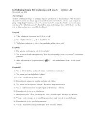
The observed errors <strong>for</strong> the <strong>splitting</strong>s Ψ h (1/3), Φ h , Φ h (1,2) and Φ h (1,3), are<br />
presented in Figure 5.1, and the corresponding <strong>order</strong>s are given in Table 5.2. The<br />
simulations clearly display that the classical <strong>order</strong> p is obtained <strong>for</strong> all <strong>methods</strong> in<br />
the cases PER and DEG, hence, in full agrement with Theorem 3.1. As discussed<br />
in Section 4, Assumption 3.2 is in general not satisfied <strong>for</strong> the infinite dimensional<br />
operator L when one imposes boundary conditions, and the convergence <strong>order</strong> is then<br />
no longer guarantied. With this in mind, it comes as no surprise that we observe severe<br />
<strong>order</strong> reductions in the experiments with DIR and NEU. More precisely, schemes with
14 Eskil Hansen, Alexander Ostermann<br />
Periodic Experiment<br />
Degenerate Experiment<br />
10 −8<br />
10 −10<br />
1<br />
4<br />
3<br />
2<br />
10 −4<br />
10 −6<br />
1<br />
4<br />
3<br />
2<br />
||error||<br />
10 −12<br />
10 −14<br />
Ψ h<br />
(1/3)<br />
Φ h<br />
Φ h<br />
(1,2)<br />
||error||<br />
10 −8<br />
10 −10<br />
10 −12<br />
Ψ h<br />
(1/3)<br />
Φ h<br />
Φ h<br />
(1,2)<br />
10 −6 h<br />
10 −16<br />
Φ h<br />
(1,3)<br />
10 −4 10 −3 10 −2 10 −1<br />
10 −2 h<br />
10 −14<br />
Φ h<br />
(1,3)<br />
10 −4 10 −3 10 −2 10 −1<br />
Dirichlet Experiment<br />
Neumann Experiment<br />
10 −5<br />
2<br />
10 −5<br />
2<br />
10 −6<br />
1<br />
10 −6<br />
1<br />
10 −4 h<br />
||error||<br />
10 −7<br />
10 −8<br />
10 −9<br />
Ψ h<br />
(1/3)<br />
10 −4 h<br />
||error||<br />
10 −7<br />
10 −8<br />
Ψ h<br />
(1/3)<br />
10 −10<br />
10 −11<br />
Φ h<br />
Φ h<br />
(1,2)<br />
Φ h<br />
(1,3)<br />
10 −4 10 −3 10 −2 10 −1<br />
10 −9<br />
10 −10<br />
Φ h<br />
Φ h<br />
(1,2)<br />
Φ h<br />
(1,3)<br />
10 −4 10 −3 10 −2 10 −1<br />
Fig. 5.1 The observed numerical errors with respect to the discrete L 2 -norm, <strong>for</strong> a variety of <strong>splitting</strong><br />
schemes. As seen from the graphs, the full convergence <strong>order</strong>s are obtained <strong>for</strong> the periodic and degenerate<br />
problems, whereas the <strong>order</strong> is reduced <strong>for</strong> all schemes with <strong>order</strong> p ≥ 3 in the problems with Dirichlet and<br />
Neumann boundaries. Note that even though the full <strong>order</strong>s are not obtained in the Dirichlet and Neumann<br />
experiments, the high <strong>order</strong> schemes still yield significantly smaller errors when compared to the Strang<br />
<strong>splitting</strong> Φ h .
<strong>High</strong> <strong>order</strong> <strong>splitting</strong> <strong>methods</strong> <strong>for</strong> <strong>analytic</strong> <strong>semigroups</strong> <strong>exist</strong> 15<br />
Table 5.2 The observed numerical <strong>order</strong>s <strong>for</strong> a variety of <strong>splitting</strong> schemes.<br />
Periodic Experiment<br />
T/h Ψ h (1/3) Φ h Φ h (1,2) Φ h (1,3)<br />
8<br />
16 2.77 2.02 2.78 3.02<br />
32 2.82 2.00 2.82 3.29<br />
64 2.87 2.00 2.91 3.70<br />
128 2.94 2.00 2.97 3.90<br />
256 2.97 2.00 2.99 3.03<br />
512 2.93 2.00 2.95 0.21<br />
Dirichlet Experiment<br />
T/h Ψ h (1/3) Φ h Φ h (1,2) Φ h (1,3)<br />
8<br />
16 2.28 1.88 2.27 2.27<br />
32 2.28 1.93 2.27 2.28<br />
64 2.28 1.95 2.28 2.30<br />
128 2.30 1.97 2.30 2.35<br />
256 2.34 1.98 2.34 2.49<br />
512 2.43 1.99 2.47 2.83<br />
Degenerate Experiment<br />
T/h Ψ h (1/3) Φ h Φ h (1,2) Φ h (1,3)<br />
8<br />
16 2.96 1.99 2.96 3.72<br />
32 2.99 2.00 2.99 3.46<br />
64 2.99 2.00 2.99 3.48<br />
128 2.99 2.00 3.00 3.73<br />
256 3.00 2.00 3.00 3.90<br />
512 3.00 2.00 3.00 3.97<br />
Neumann Experiment<br />
T/h Ψ h (1/3) Φ h Φ h (1,2) Φ h (1,3)<br />
8<br />
16 1.80 1.71 1.83 1.73<br />
32 1.72 1.74 1.73 1.68<br />
64 1.68 1.73 1.68 1.66<br />
128 1.70 1.70 1.66 1.69<br />
256 1.81 1.69 1.69 1.84<br />
512 1.98 1.71 1.88 2.34<br />
x 10 −9<br />
6<br />
4<br />
4<br />
2<br />
x 10 −10 0<br />
3<br />
2<br />
1<br />
0<br />
0<br />
0.25<br />
0.5<br />
0.75<br />
1 0<br />
0.25<br />
0.5<br />
0.75<br />
1<br />
0<br />
0.25<br />
0.5<br />
0.75<br />
1 0<br />
0.25<br />
0.5<br />
0.75<br />
1<br />
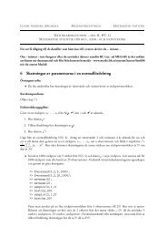
Fig. 5.2 The observed pointwise errors at time T = 0.1 <strong>for</strong> the <strong>splitting</strong> Φ h (1,3), with h = T/512, when<br />
applied to the Dirichlet (left) and Neumann (right) problems. Note how the large errors are located along<br />
a thin strip around the boundary ∂Ω.<br />
p ≥ 3 have an observed <strong>order</strong> of p ≈ 2.3 in the case of DIR, and all consider schemes<br />
have an observed <strong>order</strong> of p ≈ 1.7 <strong>for</strong> NEU.<br />
As a final remark, we would like to point out that it may still be efficient to apply<br />
exponential <strong>splitting</strong> schemes of high <strong>order</strong> to parabolic problems with boundary<br />
conditions, as they often give rise to significantly smaller errors when compared to<br />
the Strang <strong>splitting</strong> Φ h . Furthermore, the observed <strong>order</strong> reductions seem to originate<br />
only from the fact that the schemes yield large errors at, or very close to, the boundary;<br />
see Figure 5.2. Hence, the classical <strong>order</strong> is recovered sufficiently far inside the<br />
domain Ω, which can be rigorously proven by employing the techniques of [12].
16 Eskil Hansen, Alexander Ostermann<br />
However, we do not work out the details in this paper as the proof is rather lengthy<br />
and technical.<br />
References<br />
1. Bandrauk, A.D., Shen, H.: Improved exponential split operator method <strong>for</strong> solving the time-dependent<br />
Schrödinger equation. Chem. Phys. Lett. 176, 428–432 (1991)<br />
2. Blanes, S., Casas, F.: On the necessity of negative coefficients <strong>for</strong> operator <strong>splitting</strong> schemes of <strong>order</strong><br />
higher than two. Appl. Numer. Math. 54, 23–37 (2005)<br />
3. Castella, F., Chartier, P., Descombes, S., Vilmart, G.: Splitting <strong>methods</strong> with complex times <strong>for</strong><br />
parabolic equations. Preprint (2008)<br />
4. Chambers, J.E.: Symplectic integrators with complex time steps. Astron. J. 126, 1119–1126 (2003)<br />
5. Engel, K.-J., Nagel, R.: One-Parameter Semigroups <strong>for</strong> Linear Evolution Equations. Springer, New<br />
York (2000)<br />
6. Hairer, E., Lubich, Ch., Wanner, G.: Geometric Numerical Integration. Structure-Preserving Algorithms<br />
<strong>for</strong> Ordinary Differential Equations. 2nd ed., Springer, Berlin (2006)<br />
7. Hansen, E., Ostermann, A.: Exponential <strong>splitting</strong> <strong>for</strong> unbounded operators. Math. Comp. 78, 1485–<br />
1496 (2009)<br />
8. Hansen, E., Ostermann, A.: Dimension <strong>splitting</strong> <strong>for</strong> evolution equations. Numer. Math. 108, 557–570<br />
(2008)<br />
9. Hochbruck, M., Lubich, Ch.: On Krylov subspace approximations to the matrix exponential operator.<br />
SIAM J. Numer. Anal. 34, 1911–1925 (1997)<br />
10. Hundsdorfer, W., Verwer, J.: Numerical Solution of Time-Dependent Advection-Diffusion-Reaction<br />
Equations. Springer, Berlin (2003)<br />
11. McLachlan, R.I., Quispel, G.R.W.: Splitting <strong>methods</strong>. Acta Numer. 11, 341–434 (2002)<br />
12. Lubich, Ch., Ostermann, A.: Interior estimates <strong>for</strong> time discretizations of parabolic equations. Appl.<br />
Numer. Math. 18, 241–251 (1995)<br />
13. Pazy, A.: Semigroups of Linear Operators and Applications to Partial Differential Equations. Springer,<br />
New York (1983)<br />
14. Prosen, T., Pi˘zorn, I.: <strong>High</strong> <strong>order</strong> non-unitary split-step decomposition of unitary operators. J. Phys.<br />
A: Math. Gen. 39, 5957–5964 (2008)<br />
15. Schechter, M.: Principles of Functional Analysis. 2nd ed., American Mathematical Society, Providence<br />
(2001)<br />
16. Suzuki, M.: Fractal decomposition of exponential operators with applications to many-body theories<br />
and Monte Carlo simulations. Phys. Lett. A 146, 319–323 (1990)