The Information Content of Accounting Numbers as Earnings ...

Furthermore, we consider that what Ou (1990) describes as different cut-off probability schemes
(0.5, 0.5) and (0.6, 0.4) is tantamount to introducing in the outcome, besides the bias referred to
above, yet another arbitrary set of a-priori probabilities. Ou’s (1990) cut-off of 0.6 means that an
explicit prior probability is added to the logistic output. This renders the model more sensitive to
upwards earnings changes. Similarly, the cut-off of 0.4 means that a second prior judgement, contradictory
with the first, is added to the logistic regression output. Sensitivity to downwards
changes also increases. The extra power of the models may thus reflect the above prior judgements.
In order to illustrate the potential for unbalancing models which the use of non-equal priors
entails, our results are replicated using unbalanced sets of priors.. Thus, in our case, the output of
the discriminant model, a Z-score, is translated into a binary prediction of an earnings increase or
decrease, using two sets of prior probability schemes (0.5, 0.5) and (0.6, 0.4). Under the (0.5, 0.5)
scheme, earnings decreases are a-priori considered as equally likely as earnings increases. Under
the (0.6, 0.4) scheme, earnings increases are considered, a-priori, more likely, thus models are
more sensitive to positive earnings changes.
Model’s results must be validated by measuring its performance in a different data set. Ou (1990)
divided her data set in two periods, 1965-77 and 1978-83, using the first period to build the earnings
prediction model and testing its performance in the second period. However, Freeman et al.
(1982) suggest that the economy, namely macro-economic variables, may have explanatory power
in predicting earnings changes. The predictive power claimed by Ou (1990) might then stem from
smoothed economic conditions, not just from genuine accounting information. In our study, the
hypothesis that the economy may interfere with accounting information is made explicit by choosing
the period 1985-88 to build models and the period 1989-93 to test them. The first of such periods
presents economic conditions which are opposed to those in the second.
Results
Predictive Information Link: when we refer to the predictive performance of a particular year, it
means that the non-earnings accounting variables of that year are used to predict the earnings
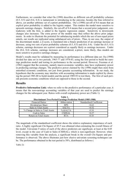
changes for the subsequent year. Ratios with overall explanatory power are (Table 1):
Table 1.
Discriminant Two-Period Earnings Prediction Model (1985-1988)
Financial Ratios Abbreviation Standardised Coefficient
Dividend per Share DPS +0.63
Sales to Total Assets SALTA +0.52
% Change in Sales to Total Assets % SALTA -0.34
Cash to Sales CSHSAL +0.27
Return on Total Assets RTA -0.18
The magnitude of the standardised coefficient shows the relative explanatory importance of each
ratio. A highly significant Chi-Square of 45.5 was obtained when estimating the overall fitness of
the model. Univariate F-ratios of each of the above predictors are significant, at least at the 0.05
level, except in the case of Cash to Sales (CSHSAL), which is non-significant. However, when
removing this variable from the analysis, a significant break in the overall Chi-Square and performance
is observed. The above illustrates just how elusive univariate screening techniques can
be. The performance obtained in the test period is 58%, distributed as follows (
Table 2):
4