The Information Content of Accounting Numbers as Earnings ...

The Information Content of Accounting Numbers as Earnings
Predictors One Year Ahead: The Case of Hong Kong
Sam Kit and Duarte Trigueiros
Faculty of Business Administration
Abstract
The study measures the power of non-earnings accounting information released by firms
in Hong Kong to predict unexpected changes in earnings and stock returns, thus replicating
an experiment carried out by Ou (1990) using US data. Our study shows that Ou’s
(1990) methodology is robust, predicting future earnings changes even where substantial
decline in economic conditions have taken place.
Introduction
Conventional wisdom in finance around the late 1980s held that stock markets in many countries
are semi-strong form efficient: stock prices impound publicly available information promptly and
without bias. Ou and Penman (1989) and Ou’s (1990) finding that publicly available financial
statement numbers can predict future abnormal stock returns was therefore striking. 1 This study
replicates, using Hong Kong data, the Ou (1990) study on the predictability of stock returns, showing
that non-earnings accounting numbers may convey information about changes in future earnings
which are not reflected in current earnings and may be used to predict future returns.
Amongst models used to explain the time series behaviour of earnings, two types have been considered:
the mean reverting type where expectations are constant over time and the stochastic type
where expectations are not stable, changing with the previous outcome, i.e., the value of a random
variable X in period t+1 is related to its value in period t as:
Xt+1 = Xt + + et
Stochastic models are similar to submartingales where = 1 and 0. X exhibits a trend whenever
is greater than 0. A martingale model, on the other hand, will be described by the same as
above with = 1 and = 0. If additionally the (et , t+1 ...., t+n) series is independently and identically
distributed, the stochastic model is a random walk.
Over the last thirty years, research has been carried out in order to ascertain which model best describes
the behaviour of earnings. Little (1962), an early study, examined the correlation between
successive growth rates in the earnings of UK firms, concluding that “the work done on correlating
past and future growth... strongly suggested that the true relationship was rather random”. The
later study of Little and Rayner (1966), again, reached the same conclusion. Lintner and Glauber
(1967) also investigated the relationship between growth rates in successive periods finding only
small cross-sectional correlation between the growth rates of successive periods. Brealey (1967;
1969) investigated changes in income instead of its growth rates concluding that income followed
a martingale. Ball and Watts (1972) examined the US Compustat firms over the 1947-1966 period
using different tests, the same inference arising from each test, that the net income and earnings
per share series follow a martingale type of process. 2
Later research, performing tests at the individual firm level leads to ambiguous evidence. Watts &
Leftwich (1977) reported that, for over half the firms in their sample, they could “reject the null
1
More recent studies such as Chan, Hamao and Lakonishok (1991), Fama and French (1993), Grieg
(1992), Stober (1992), Ou and Penman (1993) and Ball (1992) have corroborated the above results, providing
compelling evidence on the relevance of fundamental accounting variables for equity valuation.
2 In the study of Ball and Watts (1972), the actual net income data give a similar ranking to both a martingale
and a submartingale with a trend.
1

hypothesis that the estimated process is no different from a random walk at the 0.05 level”. Albrecht,
Lookabill & McKeown (1977) reported a similar result. Departures from random walk are
reported only when researchers adopt sample stratification analysis. Brooks and Buckmaster
(1976; 1980) examined a sample of US Compustat firms, stratifying their sample by the magnitude
of the previous year’s earnings change. They concluded that “a large relative increase in income is
generally followed by two or more periods when the firm underperforms the average or most likely
outcome. Likewise, a firm with a large relative decrease in income generally outperforms the average
or most likely outcome for two or more periods following the large increase”. This result
has been reported in other studies, for example, Beaver, Lambert & Morse (1980) and Freeman,
Ohlson & Penman (1982).
Instead of pursuing the path adopted by most researchers, Ou and Penman (1989) and Ou (1990)
used non-earnings accounting numbers to predict earnings changes one year ahead. Their results
provide evidence for both a “predictive information link” between some non-earnings annual report
numbers and future earnings changes and a “valuation link” between predicted future earnings
changes and stock returns during the annual report dissemination period. 3 The predictive information
link stems from fitting binary one-year-ahead earnings prediction models to selected annual
report data and comparing these models’ prediction power with that of a random walk.
Ou’s (1990) results also provide an additional explanation for a result reported in Ball and Brown
(1968). These authors noticed that the information on reported earnings is anticipated by the market
as early as 12 months prior to the preliminary earnings announcement. They speculate that
other news events, such as dividend and interim earnings announcements, might explain why “unexpected
earnings” are anticipated. The predictive information link documented in Ou’s (1990)
study suggests that the release of the previous year’s complete annual report, an event included in
Ball and Brown’s (1968) abnormal return accumulation period, provides useful information for
forming expectations about the current year’s earnings.
Ou (1990) used a dichotomous variable to predict the sign of the change in one-year-ahead earnings,
i.e., an earnings increase or an earnings decrease. A change in firm i’s earnings in year t+1,
denoted EPSit+1 is calculated as:
EPSit+1 = (EPSit+1 - EPSit) - driftit
where EPSit+1 and EPSit are firm i’s “as reported” earnings per share before extraordinary items
for years t+1 and t, respectively. The drift term for year t is defined as the mean earnings per share
change over the four years prior to year t and is required for eliminating any apparent trend in
earnings. EPSit+1 is thus an unexpected change. After fitting univariate logit models for 61 financial
ratios potentially useful as predictor candidates, only 8 such descriptors, with an estimated
coefficient significant at the 10% level, were retained. Then multivariate logit models were used
for these descriptors to find appropriate models. These descriptors are:
(1) % INVTA: percentage change in the “inventory to total assets” ratio;
(2) % SALTA: percentage growth in the “net sales to total assets” ratio;
(3) % DPS: change in “dividends per share”, relative to that of the previous year;
(4) % DEP: percentage growth in “depreciation expense”;
(5) % CPXTA1: percentage growth in the “capital expenditure to total assets” ratio;
(6) % CPXTA2: % CPXTA1, with a one-year lag;
3 In this framework, the observed contemporaneous association between accounting data and stock prices is
the result of an “information link” between accounting data and future streams of benefits from equity investments
and a “valuation link” between future benefits and stock prices. Information disclosure triggers
revisions of investors’ expectation of the future benefits. These revisions are then reflected in current stock
prices. This framework is formally presented in Ohlson (1979) and Garman and Ohlson (1980), and empirically
tested by Easton (1985).
2

(7) ROE: rate of return on equity (income before extraordinary items” divided by total
owners’ equity as of the beginning of the year);
(8) ROE: change in ROE, relative to the previous year’s ROE.
Using the above eight ratios, Ou (1990) then constructed three multivariate prediction models:
Model 1, based on all eight accounting predictors; Model 2, based on six accounting predictors
excluding ROE & % ROE; and Model 3, based on ROE only.
The predictive performance for each of the above models during the period 1978-1983 was then
examined. The output of the model is an estimated probability of an earnings increase in the subsequent
year. To translate each probabilistic prediction into a binary prediction of an earnings increase
or decrease, Ou (1990) used two pre-set probability cut-off schemes: (0.5, 0.5) and (0.6,
0.4). Under the (0.5, 0.5) scheme, the prediction is an earnings increase when the probability is
greater than 0.5 and a decrease otherwise. Alternatively, under the (0.6, 0.4) scheme, the prediction
is an earnings increase when the probability is greater than or equal to 0.6 and a decrease
when the probability is less than or equal to 0.4; observations with probability between 0.6 and 0.4
are discarded. Each of the three logit models had a prediction accuracy higher than 50% (i.e., 61%,
58% and 58% for Models 1, 2 and 3 respectively under the (0.5, 0.5) scheme). The performance
substantially improved when the (0.6, 0.4) cutoff scheme was used.
Data and Methodology
Similar to Ou’s (1990), this study approximates “unexpected earnings” in the specification of earnings
changes under a submartingale process. That is, the earnings change is defined as the difference
in two consecutive years’ earnings per share, net of estimated drift. Accounting information
used in our study is extracted from an annual Pacific-Basin Capital Markets (PACAP) Database
for the period 1985-1993 4 . Only firms not involved in banking, finance and insurance, with financial
statement figures stated in HKD and USD have been chosen. The number of firms included in
samples varies from year to year, increasing from about 215 in 1985 to 361 in 1993. Most of the
Hong Kong firms do not disclose information on Cost of Goods Sold (and consequently Gross
Margin) as they consider such information confidential and subject to usage by competitors.
Therefore, computation of ratios related to such items cannot possibly be made even though Ou
and Penman (1989) has used Gross Margin as the component predictor in their earnings prediction
model. Three other ratios also impossible to compute in our case are Percentage Change in Depreciation
(% DEP), Percentage Change in Capital Expenditure to Total Assets (% CPXTA1) and
Percentage Change in Capital Expenditure to Total Assets with a one-year lag (% CPXTA2) due
to the fact that Depreciation and Capital Expenditure are not available in the PACAP database.
These three ratios are also predictors in Ou’s (1990) models. Another problem encountered in our
study is the fact that a significant number of Hong Kong firms have zero inventory figures. This is
typical of firms such as shipping, property development and other services. Accordingly, ratios
related to Inventory were excluded from the analysis. One other ratio removed from the model due
to the large amount of missing cases is Percentage Change in Dividend Per Share (% DPS).
Except in the case of those ratios close to normality, we applied symmetrical logarithm transformations
to eliminate skewness, reduce the number of outliers and subdue heteroscedasticity. The
multivariate statistical technique employed in our study to build the empirical models is discriminant
analysis. We avoided using logit regression as such tool implicitly incorporate group proportions
as present in samples in the estimation of the predicted probabilities. If, for example, firms
exhibiting positive earnings changes are more frequent in the sample than those having negative
changes, then the logistic model is biased towards more easily recognising positive changes. Discriminant
analysis separates the calculation of conditional probabilities from the introduction of
non-equal priors.
4 The PACAP database is developed by the Sandra Ann Morsilli Pacific-Basin Capital Markets Research
Centre, in the College of Business Administration at the University of Rhode Island (USA) and is updated
annually. We extend this history back to 1981 because of the requirement to estimate an earnings drift parameter
over four years. Note, however, that the earnings prediction model is estimated using data from
1985 onwards.
3

Furthermore, we consider that what Ou (1990) describes as different cut-off probability schemes
(0.5, 0.5) and (0.6, 0.4) is tantamount to introducing in the outcome, besides the bias referred to
above, yet another arbitrary set of a-priori probabilities. Ou’s (1990) cut-off of 0.6 means that an
explicit prior probability is added to the logistic output. This renders the model more sensitive to
upwards earnings changes. Similarly, the cut-off of 0.4 means that a second prior judgement, contradictory
with the first, is added to the logistic regression output. Sensitivity to downwards
changes also increases. The extra power of the models may thus reflect the above prior judgements.
In order to illustrate the potential for unbalancing models which the use of non-equal priors
entails, our results are replicated using unbalanced sets of priors.. Thus, in our case, the output of
the discriminant model, a Z-score, is translated into a binary prediction of an earnings increase or
decrease, using two sets of prior probability schemes (0.5, 0.5) and (0.6, 0.4). Under the (0.5, 0.5)
scheme, earnings decreases are a-priori considered as equally likely as earnings increases. Under
the (0.6, 0.4) scheme, earnings increases are considered, a-priori, more likely, thus models are
more sensitive to positive earnings changes.
Model’s results must be validated by measuring its performance in a different data set. Ou (1990)
divided her data set in two periods, 1965-77 and 1978-83, using the first period to build the earnings
prediction model and testing its performance in the second period. However, Freeman et al.
(1982) suggest that the economy, namely macro-economic variables, may have explanatory power
in predicting earnings changes. The predictive power claimed by Ou (1990) might then stem from
smoothed economic conditions, not just from genuine accounting information. In our study, the
hypothesis that the economy may interfere with accounting information is made explicit by choosing
the period 1985-88 to build models and the period 1989-93 to test them. The first of such periods
presents economic conditions which are opposed to those in the second.
Results
Predictive Information Link: when we refer to the predictive performance of a particular year, it
means that the non-earnings accounting variables of that year are used to predict the earnings
changes for the subsequent year. Ratios with overall explanatory power are (Table 1):
Table 1.
Discriminant Two-Period Earnings Prediction Model (1985-1988)
Financial Ratios Abbreviation Standardised Coefficient
Dividend per Share DPS +0.63
Sales to Total Assets SALTA +0.52
% Change in Sales to Total Assets % SALTA -0.34
Cash to Sales CSHSAL +0.27
Return on Total Assets RTA -0.18
The magnitude of the standardised coefficient shows the relative explanatory importance of each
ratio. A highly significant Chi-Square of 45.5 was obtained when estimating the overall fitness of
the model. Univariate F-ratios of each of the above predictors are significant, at least at the 0.05
level, except in the case of Cash to Sales (CSHSAL), which is non-significant. However, when
removing this variable from the analysis, a significant break in the overall Chi-Square and performance
is observed. The above illustrates just how elusive univariate screening techniques can
be. The performance obtained in the test period is 58%, distributed as follows (
Table 2):
4

Table 2.
Predictive Performance of Two-Period Earnings Prediction Model Without Prior Probability
As Predicted
Actual Group
Downwards EPS
Changes
Upwards EPS
Changes
Total No. of
Cases
Downwards EPS Changes 212 (58%) 157 369
Upwards EPS Changes 152 209 (58%) 361
Total No. of Cases 364 366 730
Numbers refer to cases falling inside each classification group
The model is balanced (the proportion of upwards earnings changes correctly classified is similar
to the corresponding proportion of downwards changes).
When, in the same case, different prior probabilities are introduced to translate Z-Scores into classifications
results, the balance referred to above is strongly affected. The overall performance is
55% and, in detail (Table 3):
Table 3.
Predictive Performance, Prior Probability 0.4 And 0.6
As Predicted
Actual Group
Downwards Upwards EPS Total No. of Cases
EPS Changes Changes
Downwards EPS Changes 87 (24%) 282 369
Upwards EPS Changes 48 313 (87%) 361
Total No. of Cases 135 595 730
The above strong imbalance between upwards and downwards performance is obtained by introducing
just a small amount of prior information: p=0.6 for upwards and p=0.4 for downwards. On
a yearly basis, the prediction model performs as follows (Table 4):
Table 4.
Yearly Performance by year
Prior Probability
Total No. (0.5, 0.5) (0.6, 0.4)
Year of Cases Correct Prediction Correct Prediction
No. of Cases % No. of Cases %
1989 160 93 58% 83 52%
1990 166 94 57% 87 52%
1991 196 110 56% 115 59%
1992 208 124 60% 115 55%
Overall 730 421 58% 400 55%
Under the (0.5, 0.5) scheme, the percentage of correct predictions ranges from 56% to 60%. When
priors (0.6, 0.4) are used, prediction accuracy improves for year 1991 instead of for all years as in
Ou’s (1990) study. The results indicate that the superiority of the model over the random-guess
strategy is consistent across individual years. Table 5 and 6 are further breakdowns of the correct
prediction where subsequent earnings changes are a decrease or an increase.
5

Table 5.
Yearly Performance When Subsequent Earnings Changes are a Decrease
Prior Probability
Total No. (0.5, 0.5) (0.6, 0.4)
Year of Cases Correct Prediction Correct Prediction
No. of Cases % No. of Cases %
1989 79 45 57% 17 22%
1990 85 49 58% 19 22%
1991 98 52 53% 25 26%
1992 107 66 62% 26 24%
Overall 369 212 58% 87 24%
Table 6.
Yearly Performance When Subsequent Earnings Changes are an Increase
Prior Probability
Total No. (0.5, 0.5) (0.6, 0.4)
Year of Cases Correct Prediction Correct Prediction
No. of Cases % No. of Cases %
1989 81 48 59% 66 81%
1990 81 45 56% 68 84%
1991 98 58 59% 90 92%
1992 101 58 57% 89 88%
Overall 361 209 58% 313 87%
Under the (0.5, 0.5) scheme of the two-period model, the predictive power from year to year for
downwards earnings changes shows more variability (between 53% and 62%) than for upwards
earnings changes (between 56% and 59%). When prior probability (0.6, 0.4) is used, the correction
prediction rate is only 22% to 26% for downwards earnings changes but 81% to 92% for upwards
earnings changes.
Valuation Link: this study also investigates the link between predicted earnings changes and the
behaviour of prices in the Hong Kong stock market. Following Ou (1990), the annual report of
year t is viewed as containing two signals: First, signal E indicates the direction of changes in earnings
in the current year (t). Second, signal F (forecast) corresponds to the possibility of investors
forecasting next year’s (t+1) earnings changes.
The above discriminant model is used to forecast the changes in earnings during the period 1988-
92. Two sets of firms are obtained: F+ firms with a forecasted positive change in earnings and F-
with a negative forecast. Then, four portfolios are formed: portfolio E+F+, containing firms having
positive E and F signals; and similarly, portfolio E+F-, E-F+ and E-F-. Finally, the relative
performance of each of these portfolios in the stock market is compared using the comulative abnormal
return (CAR) measurement, calculated monthly from April of year t until March of year
t+1. 5 The CAR of a portfolio held from month m to month n (both relative to month 0) has the
form: CAR mn = 1/N t i m to n (1 + e ist ) - 1 where e ist is the market model residual of
month s for firm i in year t and N is the total number of firm-year observations in each portfolio.
Both monthly returns and the index used as the independent variable in market model regressions
were extracted from the same PACAP database. Only 50 firms having fiscal year end on December
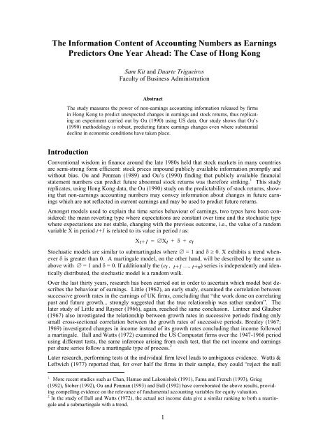
were selected, yielding a total of 250 different cases. The obtained CAR for each month are displayed
on Table 7 and in figure 1.
Table 7.
Comulative Abnormal Returns (CAR) for Portfolios and Overall
Month All Firms E-F- E+F- E-F+ E+F+
April 0.003 0.004 0.009 -0.002 0.003
5 See, e.g., Ball & Brown (1968), Ou (1990), or other texts on the absorption of information by capital markets
for more details. Notice that, in our case, CARs, not APIs (abnormal performance indices), were used.
6

May 0.022 0.024 0.040 0.015 0.030
June 0.014 0.002 0.035 -0.005 0.028
July 0.005 -0.024 0.033 -0.034 0.024
August 0.001 -0.035 0.029 -0.042 0.022
September 0.009 -0.045 0.048 -0.049 0.044
October 0.007 -0.069 0.064 -0.077 0.055
November 0.015 -0.063 0.073 -0.068 0.068
December 0.021 -0.070 0.086 -0.071 0.085
January 0.025 -0.071 0.095 -0.072 0.094
February 0.023 -0.071 0.084 -0.066 0.089
March 0.039 -0.063 0.100 -0.050 0.118
This result shows that, also in Hong Kong, investors use forecasts of changes in earnings, based on
accounting information, to price quoted firms. Indeed, during the annual report dissemination period
(January to March of year t+1), there is a change of behaviour in portfolios F+ and F- with regard
to the performance based solely on the information available for the current year (E+ or E).
The differences from Ou’s (1990) results are that, in her case, such change takes place one month
earlier and, in the case of bad news, there is no clear evidence of a post-annoncement period where
investors take a significant amount of time to absorb such news.
+.15
+.10
+.05
Figure 1. Comulative Abnormal Returns
E+F+
E-F-
E+F-
0
All Firms
-.05
E-F+
-.10
-.15
April May June July Aug. Sept. Oct. Nov. Dec. Jan. Feb. March
Conclusions
This study has replicated, in the Hong Kong context, a significant and well-known piece of research
which digs straight into the problem of whether or not accounting numbers convey significant
information to investors. Features of firms bearing significant predictive power were quite
similar in Ou’s (1990) and in our models. For example, the Percentage Change in Sales to Total
Assets (% SALTA) is exactly the same in both Ou’s (1990) and our models; the Rate of Return on
Equity (ROE) in Ou’s (1990) models is similar to our Return on Assets (RTA).
Our study confirms Ou’s basic intuition: the existence of a multivariate mechanism leading to the
predictability of firm’s earnings, small as it may be, means that investors, also in Hong Kong, can
obtain marginal information about future earnings changes. One major result of our study is the
fact that Ou’s (1990) methodology seems to be basically robust in the presence of different economic
patterns. In other words, accounting information may be used to predict, to a given extent,
earnings changes one year ahead, irrespective of the economic mood. This result importantly suggests
that, contrary to what happens in capital markets (where prices, in spite of reflecting investor’s
expectations, are very sensitive to pervasive economic forces and to specific or local events),
accounting information is more sheltered from such disturbances.
7

Bibliography
Albrecht, W. L., Lookabill L. and McKeown, J. (1977). “The Time-Series Properties of Annual Earnings”,
Journal of Accounting Research, Autumn, pp. 226-244.
Ball, R. (1992). “The Earnings-Price Anomaly” Journal of Accounting and Economics, V. 15, pp. 159-78.
Ball, R. and Brown, P. (1968). “An Empirical Evaluation of Accounting Income Numbers”, Journal of Accounting
Research, Autumn, pp. 159-178.
Ball, R. and Watts, R. (1972). “Some Time Series Properties of Accounting Income”, Journal of Finance,
June, pp. 663-681.
Brealey, R. A. (1967). “Statistical Properties of Successive Changes in Earnings”, Working paper, Keystone
Custodian Funds, March.
Brealey, R. A. (1969). “An Introduction to Risk and Return from Common Stocks”, Boston, M.I.T. Press.
Brooks, L. D. and Buckmaster D. A. (1976). “Further Evidence of the Time-Series of Accounting Income”,
Journal of Finance, December, pp. 1359-1373.
Brooks, L. D. and Buckmaster D. A. (1980). “First-Difference Signals and Accounting Income Time-Series
Properties”, Journal of Business Finance and Accounting, Autumn, pp. 437-454.
Chan, L., Yamao, Y. and Lakonishok (1991). “Fundamentals and Stock Returns in Japan”, Journal Finance,
December, pp. 1739-1764.
Easton, P. (1985). “Accounting Earnings and Security Valuation: Empirical Evidence of the Fundamental
Links”, Journal of Accounting Research, Supplement, pp. 54-77.
Fama, E. and French K. (1993) “Size and Book to Market Factors in Earnings and Returns”, Working Paper,
September.
Freeman, R., Ohlson J. and Penman S. (1982). “Book Rate-of-Return and Predictions of Earnings Changes:
An Empirical Investigation”, Journal of Accounting Research, Vol. 20, No. 2, pp. 639-653.
Garman, M. and Ohlson, J. (1980). “Information and Sequential Valuation of Assets in Arbitrage-Free Economies”,
Journal of Accounting Research, Autumn, pp. 420-440.
Grieg, A. (1992). “Fundamental Analysis and Subsequent Stock Returns”, Journal of Accounting and Economics,
Vol. 15, pp. 413-442.
Lintner, J. and Glauber, R. (1967). “Higgledy Piggledy Growth in America”, Paper presented at the Seminar
on the Analysis of Security Prices, University of Chicago, May 11-12.
Little, I. M. D. (1962). “Higgledy Piggledy Growth”, Bulletin of the Oxford Institute of Economics and Statistics,
November, pp. 387-412.
Little, I. M. D. and Rayner, A. C. (1966). “Higgledy Piggledy Growth Again”, Oxford: Basil Blackwell.
Ohlson, J. (1979). “Risk, Return, Security Valuation, and the Stochastic Behaviour of Accounting Numbers”,
Journal of Financial and Quantitative Analysis, June, pp. 317-336.
Ou, J. A. (1984). “The Information Content of Nonearnings Accounting Numbers as Earnings Predictors”,
Ph.D. dissertation, University of California, Berkeley, 1984.
Ou, J. A. (1990). “The Information Content of Nonearnings Accounting Numbers as Earnings Predictors”,
Journal of Accounting Research, Vol. 28, No. 1, Spring, pp. 392-411.
Ou, J. A. and Penman S. H. (1989) “Financial Statement Analysis and the Prediction of Stock Returns”,
Journal of Accounting and Economics, Vol. 11, pp. 295-329.
Ou, J. A. and Penman S. H. (1993) “Financial Statement Analysis and the Evaluation of Market to Book Ratios”,
Working Paper, University of California at Berkley, August.
Stober, T. (1992). “Summary Financial Statement Measures and Analysis”, Journal of Accounting and Economics,
Vol. 15, pp. 347-372.
Watts, R. and Leftwich, R. (1977). “The Time-Series Properties of Annual Earnings”, Journal of Accounting
Research, Autumn, pp. 253-271.
8