Production-Ready GPU-Based Monte-Carlo Volume Rendering

TECHNICAL REPORT, COMPUTER GRAPHICS GROUP, UNIVERSITY OF SIEGEN, 2007
Production-Ready GPU-Based Monte-Carlo Volume Rendering
Christof Rezk-Salama
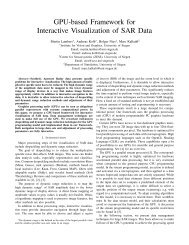
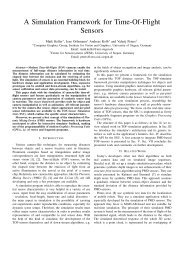
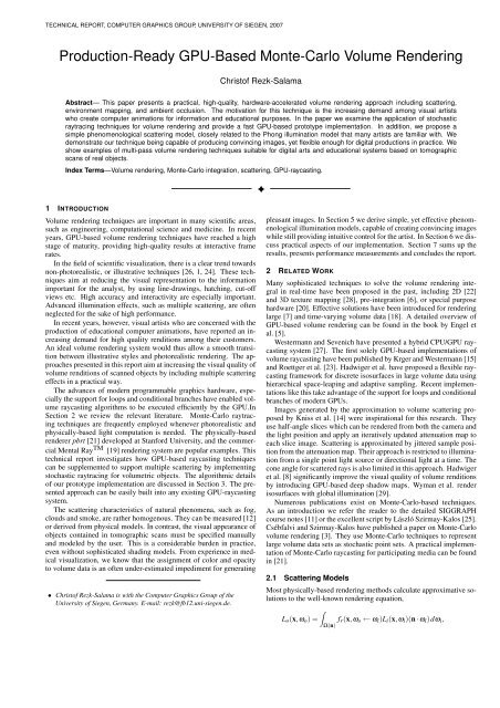
Abstract— This paper presents a practical, high-quality, hardware-accelerated volume rendering approach including scattering,
environment mapping, and ambient occlusion. The motivation for this technique is the increasing demand among visual artists
who create computer animations for information and educational purposes. In the paper we examine the application of stochastic
raytracing techniques for volume rendering and provide a fast GPU-based prototype implementation. In addition, we propose a
simple phenomenological scattering model, closely related to the Phong illumination model that many artists are familiar with. We
demonstrate our technique being capable of producing convincing images, yet flexible enough for digital productions in practice. We
show examples of multi-pass volume rendering techniques suitable for digital arts and educational systems based on tomographic
scans of real objects.
Index Terms—Volume rendering, Monte-Carlo integration, scattering, GPU-raycasting.
✦
1 INTRODUCTION
Volume rendering techniques are important in many scientific areas,
such as engineering, computational science and medicine. In recent
years, GPU-based volume rendering techniques have reached a high
stage of maturity, providing high-quality results at interactive frame
rates.
In the field of scientific visualization, there is a clear trend towards
non-photorealistic, or illustrative techniques [26, 1, 24]. These techniques
aim at reducing the visual representation to the information
important for the analyst, by using line-drawings, hatching, cut-off
views etc. High accuracy and interactivity are especially important.
Advanced illumination effects, such as multiple scattering, are often
neglected for the sake of high performance.
In recent years, however, visual artists who are concerned with the
production of educational computer animations, have reported an increasing
demand for high quality renditions among their customers.
An ideal volume rendering system would thus allow a smooth transition
between illustrative styles and photorealistic rendering. The approaches
presented in this report aim at increasing the visual quality of
volume renditions of scanned objects by including multiple scattering
effects in a practical way.
The advances of modern programmable graphics hardware, especially
the support for loops and conditional branches have enabled volume
raycasting algorithms to be executed efficiently by the GPU.In
Section 2 we review the relevant literature. Monte-Carlo raytracing
techniques are frequently employed whenever photorealistic and
physically-based light computation is needed. The physically-based
renderer pbrt [21] developed at Stanford University, and the commercial
Mental Ray TM [19] rendering system are popular examples. This
technical report investigates how GPU-based raycasting techniques
can be supplemented to support multiple scattering by implementing
stochastic raytracing for volumetric objects. The algorithmic details
of our prototype implementation are discussed in Section 3. The presented
approach can be easily built into any existing GPU-raycasting
system.
The scattering characteristics of natural phenomena, such as fog,
clouds and smoke, are rather homogenous. They can be measured [12]
or derived from physical models. In contrast, the visual appearance of
objects contained in tomographic scans must be specified manually
and modeled by the user. This is a considerable burden in practice,
even without sophisticated shading models. From experience in medical
visualization, we know that the assignment of color and opacity
to volume data is an often under-estimated impediment for generating
• Christof Rezk-Salama is with the Computer Graphics Group of the
University of Siegen, Germany. E-mail: rezk@fb12.uni-siegen.de.
pleasant images. In Section 5 we derive simple, yet effective phenomenological
illumination models, capable of creating convincing images
while still providing intuitive control for the artist. In Section 6 we discuss
practical aspects of our implementation. Section 7 sums up the
results, presents performance measurements and concludes the report.
2 RELATED WORK
Many sophisticated techniques to solve the volume rendering integral
in real-time have been proposed in the past, including 2D [22]
and 3D texture mapping [28], pre-integration [6], or special purpose
hardware [20]. Effective solutions have been introduced for rendering
large [7] and time-varying volume data [18]. A detailed overview of
GPU-based volume rendering can be found in the book by Engel et
al. [5].
Westermann and Sevenich have presented a hybrid CPU/GPU raycasting
system [27]. The first solely GPU-based implementations of
volume raycasting have been published by Krger and Westermann [15]
and Roettger et al. [23]. Hadwiger et al. have proposed a flexible raycasting
framework for discrete isosurfaces in large volume data using
hierarchical space-leaping and adaptive sampling. Recent implementations
like this take advantage of the support for loops and conditional
branches of modern GPUs.
Images generated by the approximation to volume scattering proposed
by Kniss et al. [14] were inspirational for this research. They
use half-angle slices which can be rendered from both the camera and
the light position and apply an iteratively updated attenuation map to
each slice image. Scattering is approximated by jittered sample position
from the attenuation map. Their approach is restricted to illumination
from a single point light source or directional light at a time. The
cone angle for scattered rays is also limited in this approach. Hadwiger
et al. [8] significantly improve the visual quality of volume renditions
by introducing GPU-based deep shadow maps. Wyman et al. render
isosurfaces with global illumination [29].
Numerous publications exist on Monte-Carlo-based techniques.
As an introduction we refer the reader to the detailed SIGGRAPH
course notes [11] or the excellent script by László Szirmay-Kalos [25].
Csébfalvi and Szirmay-Kalos have published a paper on Monte-Carlo
volume rendering [3]. They use Monte-Carlo techniques to represent
large volume data sets as stochastic point sets. A practical implementation
of Monte-Carlo raycasting for participating media can be found
in [21].
2.1 Scattering Models
Most physically-based rendering methods calculate approximative solutions
to the well-known rendering equation,
∫
L o (x,ω o ) = f r (x,ω o ← ω i )L i (x,ω i )(n · ω i )dω i ,
Ω(n)

TECHNICAL REPORT, COMPUTER GRAPHICS GROUP, UNIVERSITY OF SIEGEN, 2007
which is derived from the Boltzmann equations. It describes the scattering
events at a point x on a surface. L o is the outgoing radiance
which leaves the surface in direction ω o . It is computed as the integral
of the incoming radiance L i over the hemisphere Ω centered around
the surface normal n. The incoming radiance is weighted by the bidirectional
reflectance distribution function f r (BRDF) and the cosine
of the angle of incidence cosθ i = (n · ω i ). Most surface rendering
techniques assume light transport in a vacuum. In this case scattering
events are taking place at object boundaries only.
Inside of natural phenomena scattering events are considered to potentially
happen at every point inside this participating medium. In this
case, the BRDF f r is replaced by the phase function p, and incoming
radiance is integrated over the entire sphere S 2 ,
∫
L o (x,ω o ) = p(x,ω o ← ω i )L i (x,ω i )dω i .
S 2
The phase function describes the scattering characteristics of the participating
medium. The most popular phase function models are
Henyey-Greenstein, Schlick, Mie and Rayleigh (see [10, 5, 21]). Note
that the cosine term from Equation is omitted in Equation , since
the phase function directly operates on radiance values rather than differential
irradiance like the BRDF. For clarity, the optional emission
term was also omitted in Equation .
For semi-transparent surfaces, scattering events are still considered
to happen only at surface boundaries, but light can be transmitted
through transparent or translucent materials. The BRDF in Equation
is supplemented by a bidirectional transmittance distribution
function (BTDF) f t defined on the opposite hemisphere. Both the
BRDF and the BTDF are often considered together as a single bidirectional
scattering distribution function f (BSDF). The BSDF leads
to a rendering equation according to
∫
L o (x,ω o ) = f (x,ω o ← ω i )L i (x,ω i )‖(n · ω i )‖dω i ,
S 2
Material properties of translucent surfaces, such as skin or paper,
are often modeled using the bidirectional surface scattering reflectance
distribution function (BSSRDF), which require two surface
locations to be specified. A practical model has been proposed by
Jensen et al. [12]. Donner et al.[4] have supplemented this model for
multi-layered translucent materials. Interactive rendering technique
for translucent surfaces have been presented by Lensch et al. [17] and
Carr et al. [2]
The phase function can be considered as a generalization of the
BSDF. Phase functions are ideal for modeling natural phenomena.
They can be measured or derived from physical models. For objects
contained in tomographic scans, however, it is not very intuitive to
specify varying phase functions. We therefore prefer the notion of the
BSDF, since it contains the normal vector which represents the orientation
of surface-like structures. We can replace the surface normal by
the isosurface normal of the volume, which coincides with the normalized
gradient vector (except for homogenous regions).
The principle of Monte-Carlo integration is to estimate the complex
integrals from the previous section by a sum of randomized samples,
∫
S 2 g(x)dx ≈ 1 N
N g(x i )
∑
i=1 p(x i )
with x i being a random variable with probability density function
p(x i ). In practice this means that for each pixel multiple viewing rays
are cast and the radiance contributions of all rays are averaged.
3 GPU-BASED MONTE-CARLO RAYCASTING
Existing implementations of GPU-based raycasting sample the volume
successively along a viewing ray and calculate a solution of light
transfer in the absence of scattering events. If the volume data set
is represented by a 3D texture, however, we have the freedom to reflect
the ray into an arbitrary direction at any point inside the volume.
(1)
Random directions can be pre-computed, stored in additional texture
images and accessed via randomized texture coordinates.
As an initial implementation, we modify the fragment program for
GPU-raycasting to calculate the first directional derivative of the scalar
field along the viewing ray using central differences. If the magnitude
of the first derivative is larger than a specified threshold, we assume a
scattering event. We process the scattering event by obtaining a randomized
direction from a pre-computed texture and reflect the ray into
this direction. The user-specified threshold restricts scattering events
to inhomogenous regions of the volume, while rays may pass through
homogenous regions unimpededly.
We restart the fragment program for GPU-based raycasting multiple
times with different random values. The program samples the
volume at equidistant positions along the ray and integrate the phase
function while the ray travels through the volume. We will terminate
the viewing ray whenever the radiance contribution of the ray falls below
a specified threshold ε due to continuous attenuation. When the
viewing ray leaves the volume’s bounding box, the incident radiance
is sampled from an environment cube map. The accumulated radiance
RGB triplet is finally written into the frame buffer and averaged with
the previous passes.
This initial implementation has several shortcomings:
• The precomputed randomized ray directions do not account for
the directions with dominant radiance contribution. The convergence
is slow, because many rays are wasted in areas with only
little contribution.
• Many rays are terminated due to low attenuation and do not contribute
to the final image.
• The visual appearance of the volumetric object is hard to control
by the artist.
• Many calculations, such as determination of the first scattering
event, are performed repeatedly in successive passes.
The first problem is tackled by the use of importance sampling, as
described in Section 4. The second and third problems are solved
by multi-layer rendering technique which controls the reflection and
transmission events. Details for the multiple passes are explained in
Section 6.
To improve the fourth shortcoming, we use a multi-pass rendering
technique to reuse as much information as possible. In a first rendering
pass the front faces of the bounding box are rasterized. This first pass
simultaneously renders into two floating-point off-screen buffers using
the multiple-render-targets capabilities of modern GPUs. As outlined
above, the fragment shader contains a loop that successively samples
the volume along the viewing ray. The user specifies the scalar values
for a set of isosurfaces, at which scattering events should be computed.
While sampling the volume along the ray, we continuously check if
one of the specified isosurfaces was intersected. If the first isosurface
is hit, the shader breaks out of the loop.
To improve accuracy, a few iterations of interval bisection are performed
to come closer to the exact intersection point, as suggested
in [9]. The 3D texture coordinate of the intersection point is written
to the first render target. Finally, the fragment program obtains six
additional texture samples around the intersection point to estimate
the gradient vector using central differences. The gradient magnitude
is calculated, and the vector is then normalized. The orientation of
the gradient is negated if the viewing vector points into the opposite
hemisphere. In this case the gradient magnitude is also negated to keep
track of this modification. Gradient direction and magnitude are stored
as a floating-point RGBA quadruplet in the second render target and
the fragment program terminates. The contents of the two render targets
for the first-hit pass are shown in Figure 1. Successive rendering
passes start the ray integration directly at the intersection point with
the first isosurface by reading the 3D texture coordinate determined in
the first pass.

CHRISTOF REZK SALAMA: PRODUCTION-READY GPU-BASED MONTE-CARLO VOLUME RENDERING
Fig. 1. Results of the rendering passes. Far left: texture coordinate of the first isosurface hit. Left: Gradient vector of the first isosurface. Right:
Beauty pass for the first isosurface. Far right: Ambient occlusion pass for the first isosurface.
4 SAMPLING SCHEMES
Importance sampling is an effective means of increasing the rendering
performance by reducing the variance of the Monte-Carlo estimator.
More samples are placed in regions of the parameter domain where
the function to be integrated is expected to be large, while fewer samples
are used in regions where only a small contribution to the integral
is assumed. While software implementation have the flexibility to employ
arbitrary probability distributions and tailor them to the specific
integrand in Equation 1, our GPU-based implementation must work
with the same probability distribution for all scattering events due to
the parallel nature of fragment programs.
We decided to use random directions uniformly distributed on the
unit sphere as basis and employ simple but effective strategies to omit
regions with only little contribution according to the phase function
or BSDF. To avoid the necessity to account for different probability
distributions p(x), we restrict ourselves to uniform distributions. Uniform
samples are admittedly not the optimal sampling schemes, but
they allow us to remove p(x) from the sum in Equation 1 and replace
the weighted sum by a simple average for efficiency.
For a fast access to randomized direction vectors from within a fragment
shader, we use a pre-computed set of random value triplets representing
points uniformly distributed on the unit sphere. We generate
such vectors by the use of rejection sampling: We obtain triplets r S
of uniformly distributed random values in the range of [−1,1]. We
discard all vectors with a magnitude larger than 1 and normalize the
remaining vectors to unit length. The pre-computed random vectors
are stored in a 3D texture. By sampling the texture at runtime, we can
generate samples uniformly distributed on the unit sphere. Alternatively,
area-preserving parameterizations can be used to generate the
random vectors [11].
The random directions obtained from the texture can directly be
used to sample the phase function. For diffuse, surface-like reflection,
however, it is necessary to restrict the random directions to a hemisphere
centered around a given unit vector n. We can easily generate
such samples by negating all random vectors outside the given hemisphere,
r H (n) = sgn(n · r S )r S , (2)
with sgn being the signum function.
For efficiently sampling a specular Phong lobe, we need to focus
the sampling directions to a narrow cone centered around a given direction
of reflection. A simple way of focussing ray directions is to
compute a weighted sum of the hemispherical random samples r H and
the direction of perfect reflection h:
˜r P (h) = α · r H (h) + (1 − α)h.
r P (h) =
˜r P (h)
‖˜r P (h)‖
The scalar weight α determines the maximum cone angle of scattering
around the direction h. A value α = 1 means scattering in all
(3)
Fig. 2. Geometric relationship between the interpolation weight α and
the scattering cone angle γ.
directions on the hemisphere, while a value of α = 0 results in the
(non-randomized) ray direction perfectly focused into direction h.
To determine an appropriate value of α for a given specular exponent
s, we calculate the maximum reflection angle γ max , at which the
specular term falls below a user-specified threshold T (say 0.1),
Solving this equation yields
γ max (s) = max{γ | cos(γ) s > T }. (4)
γ max = arccos( s√ T ). (5)
Figure 2 illustrates the relationship between the focus weight α and
the angle γ. The maximum angle between a hemispherical sample
r H and the reflection direction h is 2 π . The interpolation according to
Equation 3 moves the point along the dotted line and the normalization
raises to interpolated point back to the hemisphere. From Figure 2, it is
easy to derive a relationship between α and the maximum angle γ max
by
α = 1 +tan(γ max − π 4 )
2
The three sampling techniques outlined in this section should be
sufficient to effectively increase the convergence of the Monte-Carlo
estimator. Importance sampling requires knowledge about the scattering
distribution at the surfaces. Which sampling strategy to use
depends, of course, on the phase function model.
5 PHASE FUNCTION MODEL
We use a simple phenomenological phase function model, which is
equal to the BSDF at specified isosurfaces and contains a simple forward
peak otherwise. The parameters of this phase function model are
(6)

TECHNICAL REPORT, COMPUTER GRAPHICS GROUP, UNIVERSITY OF SIEGEN, 2007
g
v
diffuse
reflection
r
specular
reflection
-v
transmission
g
v
r
-v
t
-g
Fig. 3. Illustration of the diffuse, specular and transmissive scattering
component of our phenomenological phase function model without refraction
left and with refraction right.
derived from the underlying scalar field s(x). To keep the model controllable
by the user, we restrict scattering events to happen at a fixed
set of isosurfaces. Between these isosurfaces the ray direction does
not change, but attenuation may still happen:
L(x + ∆x) = τ(s(x))L(x). (7)
The radiance L is multiplied by an attenuation coefficient τ(s) as it
travels through the volume. Attenuation τ is either constant (say 0.99)
or obtained by a user-specified transfer function.
At the specified isosurfaces, the gradient magnitude ∇s(x) is guaranteed
to be non-zero. The gradient vector is normalized and its orientation
is adjusted to match the viewing direction. As in most illumination
models we assume the viewing vector v to point towards the eye
position.
⎧
⎨
g(x) =
⎩
∇s(x)
‖∇s(x)‖ if ∇s(x) · v ≥ 0
− ∇s(x)
‖∇s(x)‖ if ∇s(x) · v < 0
Our phenomonological BSDF is illustrated in Figure 3. The reflective
part f r is equal to the specular and diffuse term of the Phong local
illumination model,
f r = f diff + f spec (9)
f diff (v ← ω i ) = k d (n · ω i ) (10)
f spec (v ← ω i ) = k s (r · ω i ) s (11)
with r = 2n(n · v) − v. (12)
The transmissive part scatters the transmitted light in an additional
Phong lobe centered around the negative viewing vector -v in case of
non-refractive transmission,
(8)
f t (v ← ω i ) = k t (−v · ω i ) q . (13)
For refractive transmission, the Phong lobe is centered around the refracted
ray direction t (Figure 3, right). In this case the refracted vector
t is calculated according to Snell’s law and replaces −v in Equation 13.
Figure 4 shows the influence of the exponent q for the transmission
lobe.
The resulting BSDF model has 5 parameters to adjust for each specified
isosurface: the diffuse, specular and transmissive material coefficients
k d , k s and k t and the exponents s and q for the specular and
transmissive lobe.
In practice, we decide for each pass which kind of scattering event
we will calculate at which intersection point. We differentiate between
diffuse reflection, specular reflection and transmission, and choose the
respective sampling scheme from Equation 2 and 3. We vary these
decisions for successive passes and this allows us to adjust the computation
time spent for each type of reflection according to the convergence
and the contribution on the final image. If specular or transmissive
scattering is computed, the interpolation weights α are calculated
from the Phong lobe exponents q and s.
Fig. 4. UTCT Salamander head rendered with different exponents q for
the transmission lobe.
Although the raycasting algorithm does not depend on it, the material
coefficients k d , k s and k t should be chosen not to violate the laws of
energy conservation. These coefficients can also be controlled by other
parameters, such as a Fresnel term, or the gradient magnitude of the
isosurface. As an example Figure 5 shows an opaque isosurface with a
specular exponent s proportional to the gradient magnitude. This renders
regions highly reflective where the gradient is steep because the
the bone is close to the skin.
6 A PRACTICAL EXAMPLE
In this section we report about practical experiences with the proposed
Monte-Carlo volume raycasting system and show some examples of
how to generate production-quality renditions.
In digital production it turns out to be advantageous to decompose
the final rendering into different independent layers. Although this
often leads to physically incorrect solutions, it allows the artist to adjust
contrast and brightness of different layers without the necessity to
recompute a single frame of image material.
The most important scattering events are the first two. In many
cases not more than one transparent layer must be considered.
Throughout our experiments we did not find volume data sets where
more than two transparent isosurfaces can be simultaneously perceived
clearly.
6.1 Isosurface Beauty Pass
In practice, we calculate the first-hit pass as outlined in Section 3. The
next pass is a beauty pass for the first isosurface (Figure 6,B). We read
the gradient direction g from target 1 of the first pass and sample the

CHRISTOF REZK SALAMA: PRODUCTION-READY GPU-BASED MONTE-CARLO VOLUME RENDERING
A B C D E
Fig. 6. Illustration of different rendering passes. A: First hit pass. B: Isosurface Beauty Pass. C: Ambient Occlusion Pass. D: Subsurface Scattering
Pass (Accurate Version). E: Subsurface Scattering Pass (Fast Version).
Fig. 7. UTCT Cheetah skull (512 3 , 16bit). Isosurface with Phong illumination
and Ambient occlusion, illuminated by LDR-version of the Grace
Cathedral cube map.
preview images at interactive frame rates. For more information on
performance we refer to Section 7.
The third image from left in Figure 1 shows the result of the beauty
pass for the UTCT Veiled Chameleon data set illuminated by the LDRversion
of the Grace cathedral environment map (courtesy of Paul Debevec,
www.debevec.org). Since light is additive, for maximum flexibility
in the compositing step, we can as well render separate diffuse
and specular passes. This allows us to adjust the specular and diffuse
reflection coefficients later in the compositing step.
Fig. 5. UTCT Veiled Chameleon: Opaque isosurface rendered with a
specular exponent s proportional to the gradient magnitude.
environment cube map directly multiple times to calculate local diffuse
and specular illumination. Alternatively, the environment map
can be pre-filtered to generate an irradiance map for the diffuse term
or a reflection map for the specular term [13]. This, of course would
be more efficient because the environment map must be sampled only
once. However, it does not allow us to use different specular exponents
simultaneously as in Figure 5. Before the fragment program for
this first isosurface pass exits, it calculates the Fresnel term from the
gradient and viewing vector and stores it in the alpha portion of the
frame buffer. The Fresnel term is for probably needed later during
compositing.
One advantage of Monte-Carlo based raycasting is that it allow us
to easily render in preview quality simply by decreasing the number
of rays per pixel. Thus we can generate still noisy, but representative
6.2 Ambient Occlusion
For rendering soft shadows, ambient occlusion [16, 30] has become
very popular in many digital productions in the recent years. Ambient
occlusion is an essential way to fake global illumination effects, resulting
in images similar to radiosity calculations, but at considerably
lower computational cost.
The idea of ambient occlusion is to calculate an “accessibility”
value for each surface point by casting rays in directions randomly
scattered across the hemisphere centered around the normal. We simply
maintain a counter of how many of the sent rays intersect the
geometry. The percentage of rays leaving the point without intersecting
geometry determines the brightness of the point.
Ambient occlusion can easily be calculated for isosurfaces using
our Monte-Carlo raycaster (Figure 6,C). For an ambient occlusion pass
we read again the position and gradient vector generated in the first
pass. For each pixel we cast several rays from the isosurface across
the hemisphere centered around the gradient direction. The rays are
traced only a few steps using a large step size to determine whether

TECHNICAL REPORT, COMPUTER GRAPHICS GROUP, UNIVERSITY OF SIEGEN, 2007
they hit the isosurfaces again or not. The percentage of rays which do
not hit the geometry are stored as grayvalue in the frame buffer. The
rightmost image in Figure 1 shows the result of the ambient occlusion
pass.
Multiplying the beauty pass by an ambient occlusion pass already
result in photorealistic isosurface rendering as displayed in Figure 7.
For higher accuracy, the bent normal, which is the average of all ray
directions that do not hit the geometry, can be used instead of the gradient
direction for the diffuse term. The top left image in Figure 9
shows the results for the skin of the Veiled Chameleon.
6.3 Subsurface Scattering
In practice, a single subsurface scattering pass turned out to be sufficient
in most cases. This means that we start a transmissive ray at
the hit point with the first isosurface. The direction is scattered within
a Phong lobe around the negative viewing direction or the refracted
vector (Figure 6,D). We trace this ray by accumulating the attenuation
factors until it hits the second isosurface. At this second hit point, the
gradient vector is estimated and the ray is reflected randomly into the
hemisphere centered around the gradient direction. The ray is traced
with attenuation but without further scattering until it leaves the volume.
If it hits another isosurface, the ray is attenuated by the phase
function, but does not change direction. This strategy avoids rays being
reflected again and again until their contribution becomes zero due
to attenuation.
A faster version (Figure 6,E) of this scattering pass is based on the
assumption that the attenuation which is accumulated from the eye
point to the second hit point is an appropriate estimate for the attenuation
from the hit point back to the outside. Hence, we can square
the accumulated attenuation and directly sample the environment map
in the reflected direction without tracing the ray any further. Although
less accurate, this technique is much faster because we can sample the
environment map many times at the second hit point to directly estimate
diffuse and specular reflection.
Our experiments have shown that there is little visible difference
if we compare images generated by the more accurate and the faster
method. We expect however, that this is due to the onion-like structure
of isosurfaces and should not be generalized to arbitrary surfaces
inside the volume. The top right image of Figure 9 shows the result of
the subsurface scattering pass for the Veiled Chameleon.
6.4 Compositing
If all the separate passes are rendered, the final image can be generated.
If multiple layered subsurface scattering passes are computed
they should be composited separately in back-to-front order. The isosurface
beauty pass should be multiplied with the ambient occlusion
pass and blended on top of the subsurface scattering pass using the
Fresnel term or the first isosurface’s opacity as blending weight. The
large image in Figure 9 shows the final compositing result of the UTCT
Veiled Chameleon.
7 RESULTS AND CONCLUSION
The presented Monte-Carlo volume raycasting approach has been
implemented using Cg (nv40 profile) and OpenGL on an NVidia
Geforce 8800 GTX graphics board with 768 MB video memory. The
rendering techniques have been evaluated using data sets from the
DigiMorph/UTCT data archive at the University of Texas at Austin
(utct.tacc.utexas.edu).
The GPU-based implementation of the Monte-Carlo raycaster does
not maximize the efficiency using stratified sampling or importance
sampling, like many software implementations do. Nevertheless, the
high parallel architecture of the GPU generates images at considerable
speed.
The convergence of the proposed technique greatly depends on the
phase function used. We have experimented with different phase functions
and found that allowing scattering events to happen at every
point inside the volume leads to extremely slow convergence and is
thus computationally not feasible. The resulting images are hardly
Pass Samples Time/msec
First Hit pass - 45–50
Iso Beauty (P) 16 spec., 8 diff. 80–170
Amb.Occ. (P) 32 rays, 10 steps 120–170
Sub.Scat. (P) 4 prim., 4 sec. 210–470
Final (P) see individual passes 598–690
Iso Beauty 128 spec., 64 diff. 274–349
Amb.Occ. 128 rays, 20 ray steps 1450–1876
Sub.Scat. 64 prim., 16 sec. 5968–8771
Final see individual passes 7156–9203
Table 1. Performance measurement for different passes in preview (P)
and final quality.
predictable for the artist, which leads to visual parameters being impossible
to control in practice. This is the reason, why we suggest
restricting the scattering events to a limited set of isosurfaces. As with
many practical computer graphics techniques our aim is not to maintain
physical correctness at the cost of usability.
Up until now we did not consider light being emitted by the volume
itself. Neither did we implement importance sampling for the
environment map, which is necessary to efficiently use high dynamic
range environment maps. We leave these aspects as a future work.
The performance of the different passes is shown in Table 1. Performance
was measured both for preview (P) and final quality. The
results show that preview renderings of the single passes are possible
at interactive frame rates, which is important to adjust visual parameters
in practice. The results of the preview passes are still noisy, but
the image quality is good enough to get the visual impression of the
final result. Comparison between preview and final images for the isosurface
beauty pass and the subsurface scattering pass are shown in
Figure 8.
The rendering performance did not significantly depend on the size
of the volume as long as it fits into the graphics memory. This is
an indication that the process is clearly fragment-processor-limited.
The performance greatly benefits from the unified shader model, since
the load on the vertex processor is negligible. Experiments on other
graphics hardware prove this.
The first conclusion we draw is that, in practice, the rendering of
volumetric objects with observable internal structures, such as the tomographic
scans used throughout this report, requires considerably
different strategies than rendering typical translucent materials, such
as clouds, milk and skin, where scattering is rather homogenous. The
method described in this technical report is meant as a proof of concept.
The multi-layer rendering technique exemplified in Section 6
only represents one way of applying the described techniques. Another
conclusion we draw from our experiments is that scattering
passes must be tailored to the desired visual effect. Multiple scattering
layers may be used and viewing rays may be transmitted through the
entire volume to account for translucency effects for backlit objects
and the like. The described techniques integrate well in the layered
shading framework well known to visual artists. Since the rendering
parameters are derived from the Phong model, they are intuitive to
control and already familiar to most artists. We have presented a practical
solution for rendering high quality images of tomographic scans
including subsurface scattering effects.
REFERENCES
[1] S. Bruckner, S. Grimm, A. Kanitsar, and E. Gröller. Illustrative Context-
Preserving Volume Rendering. In Proceedings of EuroVis 2005, pages
69–76, 2005.
[2] N. Carr, J. Hall, and J. Hart. GPU Algorithms for Radiosity and Subsurface
Scattering. In Proc. Graphics Hardware, 2003.
[3] B. Csébfalvi and L. Szirmay-Kalos. Monte carlo volume rendering. In
Proc. IEEE Visualization, 2003.
[4] C. Donner and H. W. Jensen. Light Diffusion in Multi-Layered Translucent
Materials. In Proc. ACM SIGGRAPH, 2005.

CHRISTOF REZK SALAMA: PRODUCTION-READY GPU-BASED MONTE-CARLO VOLUME RENDERING
Preview (120ms)
Final (349 ms)
Preview (470 ms)
Final (6129 ms)
Fig. 8. Comparison between preview quality and final result for the isosurface pass and the subsurface scattering pass.
[5] K. Engel, M. Hadwiger, J. Kniss, C. Rezk-Salama, and D. Weiskopf.
Real-Time Volume Graphics. AK Peters, Ltd., 2006.
[6] K. Engel, M. Kraus, and T. Ertl. High-Quality Pre-Integrated Volume
Rendering Using Hardware-Accelerated Pixel Shading. In Proceedings of
ACM SIGGRAPH/Eurographics Workshop on Graphics Hardware, 2001.
[7] S. Guthe, M. Wand, J. Gonser, and W. Straßer. Interactive Rendering of
Large Volume Data Sets. In Proceedings of IEEE Visualization, pages
53–60, 2002.
[8] M. Hadwiger, A. Kratz, C. Sigg, and K. Bhler. Gpu-accelerated deep
shadow maps for direct volume rendering. In Proc. Graphics Hardware,
2006.
[9] M. Hadwiger, C. Sigg, H. Scharsach, K. Bühler, and M. Gross. Real-
Time Ray-Casting and Advanced Shading of Discrete Isosurfaces. In
Proceedings of Eurographics, pages 303–312, 2005.
[10] L. Henyey and J. Greenstein. Diffuse radiation in the galaxy. Astrophysical
Journal, pages p. 70–83, 93.
[11] H. W. Jensen, J. Arvo, P. Dutre, A. Keller, A. Owen, M. Pharr, and
P. Shirley. Monte carlo ray tracing. In ACM SIGGRAPH Course Notes
44, 2003.
[12] H. W. Jensen, S. R. Marschner, M. Levoy, and P. Hanrahan. A Practical
Model for Subsurface Light Transport. In Proceedings of ACM SIG-
GRAPH, pages 511–518, 2001.
[13] J. Kautz and M. McCool. Approximation of glossy reflection with prefiltered
environment maps. In Proc. Graphics Interface, 2000.
[14] J. Kniss, S. Premoze, C. Hansen, and D. Ebert. Interative Translucent
Volume Rendering and Procedural Modeling. In Proceedings of IEEE
Visualization, 2002.
[15] J. Krüger and R. Westermann. Acceleration Techniques for GPU-based
Volume Rendering. In Proceedings of IEEE Visualization 2003, pages
287–292, 2003.
[16] H. Landis. Production-ready global illumination. In ACM SIGGRAPH
Course Notes 16, 2002.
[17] H. Lensch, M. Goesele, P. Bekaert, J. Kautz, M. Magnor, J. Lang, and H.-
P. Seidel. Interactive rendering of translucent objects. Computer Graphics
Forum, 22(2), 2003.
[18] E. B. Lum, K. L. Ma, and J. Clyne. Texture Hardware Assisted Rendering
of Time-Varying Volume Data. In Proceedings of IEEE Visualization,
pages 263–270, 2001.
[19] Mental Images, Inc. Mental ray rendering system.
http://www.mentalimages.com/. (last visited 2007/02/08).
[20] H. Pfister, J. Hardenbergh, J. Knittel, H. Lauer, and L. Seiler. The
VolumePro real-time ray-casting system. In Proceedings of ACM SIG-
GRAPH, pages 251–260, 1999.
[21] M. Pharr and G. Humphreys. Physically Based Rendering - From Theory
To Implementation. Morgan Kauffman/Elsevier, 2004.
[22] C. Rezk-Salama, K. Engel, M. Bauer, G. Greiner, and T. Ertl. Interactive
Volume Rendering on Standard PC Graphics Hardware Using Multi-
Textures and Multi-Stage Rasterization. In Proceedings of ACM SIG-
GRAPH/Eurographics Workshop on Graphics Hardware, 2000.
[23] S. Röttger, S. Guthe, D. Weiskopf, and T. Ertl. Smart Hardware-
Accelerated Volume Rendering. In Procceedings of EG/IEEE TCVG
Symposium on Visualization VisSym ’03, pages 231–238, 2003.
[24] N. Svakhine, D. Ebert, and D. Stredney. Illustration motifs for effective
medical volume illustration. IEEE Computer Graphics and Applications,
25(3):31–39, May 2005.
[25] L. Szirmay-Kalos. Monte-carlo methods in global illumination.
http://www.iit.bme.hu/ szirmay/script.pdf, 1999. Script, Institute of Computer
Graphics, Vienna University of Technology.
[26] I. Viola, A. Kanitsar, and E. Gröller. Importance-Driven Volume Rendering.
In Proceedings of IEEE Visualization, pages 139–145, 2004.
[27] R. Westermann and B. Sevenich. Accelerated volume raycasting using
texture mapping. In Proc. IEEE Visualization, 2001.
[28] O. Wilson, A. V. Gelder, and J. Wilhelms. Direct Volume Rendering via
3D-textures. Technical Report UCSC-CRL-94-19, Univ. of California,
Santa Cruz, 1994.
[29] C. Wyman, S. Parker, P. Shirley, and C. Hansen. Interactive Display of
Isosurfaces with Global Illumination. IEEE Transactions on Visualization
and Computer Graphics, 12(2):186–196, 2006.
[30] S. Zhukov, A. Iones, and G. Kronin. An ambient light illumination model.
In Proc. Eurographics Rendering Workshop, 1998.

TECHNICAL REPORT, COMPUTER GRAPHICS GROUP, UNIVERSITY OF SIEGEN, 2007
Fig. 9. Top left: First-Hit isosurface beauty pass with ambient occlusion with 64 diffuse, 128 specular and 128 ambient occlusion rays per pixel
rendered in 500ms. Top right: Subsurface scattering pass with 64 primary and 16 secondary rays rendered in 700 ms. Bottom: Final composite
rendered in 1200 ms. The transparency is determined by the Fresnel term of the first isosurface.