Miguel A. Diaz , Koichi Kusunoki , and Akira Tasai

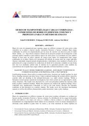
Table 1 Characteristics of specimens
Specimen
Thickness
1 st F
column
(mm)
Height
1 st F
(mm)
Total
weight
(kN)
Natural
period
(s)
Yield.
Disp.
(mm)
Frame1 a 4.5 805 1.450 1.03 66
Frame2 a, b 4.5 1005 1.464 1.66 101
S-F 01, 02, 03 6.0 1000 1.485 0.93 71
S-S 01, 02 6.0 1000 1.485 0.99 73
S-S 03, 04 6.0 1000 1.485 0.98 73
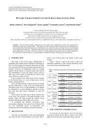
a) Velocity response spectra
The measurement system was given by accelerometers
at the base and beams of each level, and displacement
transducers connected at each eastern rigid joint, as shown in
Figure 3.
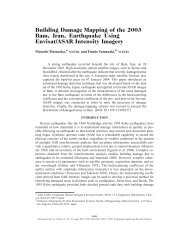
3.2 Input waveforms
The input motions to conduct this study were one
artificial wave: the WG60, and two earthquake records: the
KOBE-NS (Kobe, 1995) and the MYG013 (Tohoku, 2011).
The input motions were scaled in order to induce different
performance levels on the specimen within elastic and
inelastic ranges, both mainshocks and aftershocks. Figure 4
shows the WG60, the KOBE-NS and the MYG013
waveforms.
b) Displacement and acceleration response spectra
Figure 5 Response spectra
3.3 Equivalent SDOF
In order to conduct the residual seismic performance
analysis, it is necessary to transform the capacity curve of
the specimen in terms of S a − S d relations.
The probable value of the maximum response is usually
given by the square root of the sum of square (SRSS) of the
maximum modal response components. Then the maximum
displacement at i-th story and the base shear force can be
expressed approximately by Eq. (5) and Eq. (6) (Shibata,
2010), respectively; where s S d , s S a is the spectral
displacement and spectral acceleration for the s-th mode.
The base shear force of N-DOF is given by Eq. (7).
|δ i | max ≈ √∑
N
| s β ∙ s u i ∙ S d
s | 2
S=1 (5)
Figure 4 Input waveforms
Figure 5 shows their respective a) normalized velocity
response spectra respect to the maximum spectral velocity,
and b) normalized response spectra respect to peak ground
acceleration (PGA) and maximum spectral displacement.
The maximum spectral response with viscous damping ratio
of 0.05 was obtained at periods of 1.27 seconds, 0.87
seconds and 0.67 seconds for the WG60, the KOBE-NS and
the MYG013 waveforms, respectively (Figure 5a).
N N
S=1 i=1
+ (6)
Q ≈ √∑ *∑ m i ∙ s β ∙ s u i ∙ s S a
N
Q = ∑i=1 m i ∙ (ẍ i + ẍ g) (7)
Particularly, the specimens can be assumed as 3-DOF
systems. Their configuration allows that second and third
participation factor can be neglected, and the first-mode
distribution can be assumed as the unit { 1 u} ≈ *1+. Then
Eq. (5) is rewritten as Eq. (8) to calculate the spectral
acceleration, and Eq. (7) into Eq. (6) is rewritten as Eq. (9) to
calculate the spectral displacement.
- 1206 -