Camera Calibration Based on 2D-plane - Academy Publisher

B. Solve camera parameter matrix
The solution of the camera parameter matrix can be
seen Literature[6].
III. EXPERIMENT AND RESULTS
A. Experiment materials
KOKO camera; Image gathering card; Computer;
Tripod; 7×9 the black and white interaction's chess
discoid grid 2D plane target (as shown in Figure 1), each
grid size for 28×28 millimeter; Horizontal iron sheet
Figure 2. <strong>Calibration</strong> with the 25 images
Figure 1. 2D plane for camera calibration
B. Experiment procedure
1) Prints a calibration template to paste on the
horizontal iron sheet;
2) moves plane or camera to shot some template
images (more than or equal 20)from different angle;
3) detects characteristic point of the image;
4) obtains each image the unitary matrix H ;
5) computes camera's internal parameter by using
matrix H extracted in the premise of the distortion factor
being zero;
6) obtains a group of precision higher camera's
internal parameter by Further optimizing using the
counter-projection, simultaneously calculating each
distortion factor.
C. Experimental results
1) Lens' internal parameter
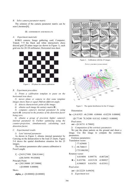
As shown in Figure 2, obtains internal parameter by
Carrying on the demarcation to the load 25 charts. Figure
5-8 shows the spatial distribution situation for the 25
images.
The intrinsic parameters after camera calibration is
Focal Length:
f = c
[3419.27498 3260.81444 ]
±[88.56950 99.83080]
Principle Point:
cc = [383.50000 287.50000]
± [0.00000 0.00000]
Skew:
alpha_c = [0.00000] ± [0.00000]
Figure 3. The spatial distribution for the 25 images
Distortation:
kc = [-0.41925 -46.21000 -0.00466 -0.02250 0.00000]
± [0.77140 78.34200 0.01162 0.00423 0.00000]
Pixel error:
err = [0.36731 0.79805]
2) Computation of the extrinsic parameters
We put the plane pattern on the ground and shoot a
image. Use this image to compute the extrinsic
parameters.
Extrinsic parameters:
Translation vector:
⎡-77.629688
⎤
T =
⎢
-98.708815
⎥
⎢ ⎥
⎢⎣
1755.086388⎥⎦
Rotation vector:
⎡ 0.019894 0.999776 -0.007244⎤
R =
⎢
0.433706 -0.015158 -0.900927
⎥
⎢ ⎥
⎢⎣
-0.900835 0.014781 -0.433911⎥⎦
Pixel error:
err = [0.32229 0.69439]
3) Experiment test
366