Download Full Journal - Pakistan Academy of Sciences
Download Full Journal - Pakistan Academy of Sciences
Download Full Journal - Pakistan Academy of Sciences

You also want an ePaper? Increase the reach of your titles
YUMPU automatically turns print PDFs into web optimized ePapers that Google loves.
ISSN Print : 0377 - 2969<br />
ISSN Online : 2306 - 1448<br />
Vol. 49(4), December 2012
PAKISTAN ACADEMY OF SCIENCES<br />
Founded 1953<br />
President: Atta-ur-Rahman .<br />
Secretary General: G.A. Miana<br />
Treasurer: Shahzad A. Mufti<br />
Proceedings <strong>of</strong> the <strong>Pakistan</strong> <strong>Academy</strong> <strong>of</strong> <strong>Sciences</strong>, published since 1964, is quarterly journal <strong>of</strong> the <strong>Academy</strong>. It publishes<br />
original research papers and reviews in basic and applied sciences. All papers are peer reviewed. Authors are not required to<br />
be Fellows or Members <strong>of</strong> the <strong>Academy</strong>, or citizens <strong>of</strong> <strong>Pakistan</strong>.<br />
Editor-in-Chief:<br />
Abdul Rashid, <strong>Pakistan</strong> <strong>Academy</strong> <strong>of</strong> <strong>Sciences</strong>, 3-Constitution Avenue, Islamabad, <strong>Pakistan</strong>; pas.editor@gmail.com<br />
Editors:<br />
Engineering <strong>Sciences</strong> & Technology: Abdul Raouf, 36-P, Model Town, Lahore, <strong>Pakistan</strong>; abdulraouf@umt.edu.pk<br />
Life <strong>Sciences</strong>: Kauser A. Malik . , Forman Christian College (a Chartered University), Lahore, <strong>Pakistan</strong>; kauser45@gmail.com<br />
Medical <strong>Sciences</strong>: M. Salim Akhter, 928, Shadman Colony-I, Lahore-54000, <strong>Pakistan</strong>; msakhter47@yahoo.com<br />
Physical <strong>Sciences</strong>: M. Aslam Baig, National Center for Physics, Quaid-i-Azam University Campus, Islamabad, <strong>Pakistan</strong>;<br />
baig@qau.edu.pk<br />
Editorial Advisory Board:<br />
Syed Imtiaz Ahmad, Computer Information Systems, Eastern Michigan University, Ypsilanti, MI, USA; imtiaz@cogeco.ca<br />
Niaz Ahmed, National Textile University, Faisalabad, <strong>Pakistan</strong>; rector@ntu.edu.pk<br />
M.W. Akhter, University <strong>of</strong> Massachusetts Medical School, Boston, MA, USA; wakhter@hotmail.com<br />
M. Arslan, Institute <strong>of</strong> Molecular Biology & Biotechnology, The University <strong>of</strong> Lahore, <strong>Pakistan</strong>; arslan_m2000@yahoo.com<br />
Khalid Aziz, King Edward Medical University, Lahore, <strong>Pakistan</strong>; drkhalidaziz@hotmail.com<br />
Roger N. Beachy, Donald Danforth Plant Science Center, St. Louis, MO, USA; rnbeachy@danforthcenter.org<br />
Arshad Saleem Bhatti, CIIT, Islamabad, <strong>Pakistan</strong>; asbhatti@comsats.edu.pk<br />
Zafar Ullah Chaudry, College <strong>of</strong> Physicians and Surgeons <strong>of</strong> <strong>Pakistan</strong>, Karachi, <strong>Pakistan</strong>; publications@cpsp.edu.pk<br />
John William Christman, Dept. Medicine and Pharmacology, University <strong>of</strong> Illinois, Chicago, IL, USA; jwc@uic.edu<br />
Uri Elkayam, Heart Failure Program, University <strong>of</strong> Southern California School <strong>of</strong> Medicine, LA, CA, USA; elkayam@usc.edu<br />
E.A. Elsayed, School <strong>of</strong> Engineering, Busch Campus, Rutgers University, Piscataway, NJ, USA; elsayed@rci.rutgers.edu<br />
Tasawar Hayat, Quaid-i-Azam University, Islamabad, <strong>Pakistan</strong>; t_pensy@hotmail.com<br />
Ann Hirsch, Dept <strong>of</strong> Molecular, Cell & Developmental Biology, University <strong>of</strong> California, Los Angeles, CA, USA; ahirsch@ucla.edu<br />
Josef Hormes, Canadian Light Source, Saskatoon, Saskatchewan, Canada; josef.hormes@lightsource.ca<br />
Fazal Ahmed Khalid, Pro-Rector Academics, GIKI, TOPI, <strong>Pakistan</strong>; khalid@giki.edu.pk<br />
Abdul Khaliq, Chairman, Computer Engineering, CASE, Islamabad, <strong>Pakistan</strong>; chair-ece@case.edu.pk<br />
Iqrar Ahmad Khan, University <strong>of</strong> Agriculture, Faisalabad, <strong>Pakistan</strong>; mehtab89@yahoo.com<br />
Asad Aslam Khan, King Edward Medical University, Lahore, <strong>Pakistan</strong>; kemcol@brain.net.pk<br />
Autar Mattoo, Beltsville Agricultural Research Center, Beltsville, MD, USA; autar.mattoo@ars.usda.gov<br />
Anwar Nasim, House 237, Street 23, F-11/2, Islamabad, <strong>Pakistan</strong>; anwar_nasim@yahoo.com<br />
M. Abdur Rahim, Faculty <strong>of</strong> Business Administration, University <strong>of</strong> New Burnswick, Fredericton, Canada; rahim@unb.ca<br />
M. Yasin A. Raja, University <strong>of</strong> North Carolina, Charlotte, NC, USA; raja@uncc.edu<br />
Martin C. Richardson, University <strong>of</strong> Central Florida, Orlando, FL, USA; mcr@creol.ucf.edu<br />
Hamid Saleem, National Centre for Physics, Islamabad, <strong>Pakistan</strong>; hamid.saleem@ncp.edu.pk<br />
Annual Subscription for 2012: <strong>Pakistan</strong>: Institutions, Rupees 2000/- ; Individuals, Rupees 1000/-<br />
Other Countries: US$ 100.00 (includes air-lifted overseas delivery)<br />
© <strong>Pakistan</strong> <strong>Academy</strong> <strong>of</strong> <strong>Sciences</strong>. Reproduction <strong>of</strong> paper abstracts is permitted provided the source is acknowledged.<br />
Permission to reproduce any other material may be obtained in writing from the Editor-in-Chief.<br />
The data and opinions published in the Proceedings are <strong>of</strong> the author(s) only. The <strong>Pakistan</strong> <strong>Academy</strong> <strong>of</strong> <strong>Sciences</strong> and the<br />
Editors accept no responsibility whatsoever in this regard.<br />
HEC Recognized, Category X; PM&DC Recognized<br />
Published by <strong>Pakistan</strong> <strong>Academy</strong> <strong>of</strong> <strong>Sciences</strong>, 3 Constitution Avenue, G-5/2, Islamabad, <strong>Pakistan</strong><br />
Tel: 92-5 1-9207140 & 9215478; Fax: 92-51-9206770; Website: www.paspk.org<br />
Printed at PanGraphics (Pvt) Ltd., No. 1, I & T Centre, G-7/l, Islamabad, <strong>Pakistan</strong><br />
Tel: 92-51-2202272, 2202449 Fax: 92-51-2202450 E-mail: pangraph@isb.comsats.net.pk
C O N T E N T S<br />
Volume 49, No. 4, December 2012<br />
Page<br />
Research Articles<br />
Engineering <strong>Sciences</strong><br />
Electrochemical Behavior <strong>of</strong> Yttria Stabilized Thermal Barrier Coating on<br />
<br />
— M. Farooq, K. M. Deen, S. Naseem, S. Alam, R. Ahmad and A. Imran<br />
<br />
Life <strong>Sciences</strong><br />
<br />
— M. Jawed Iqbal, Zaeem Uddin Ali and S. Shahid Ali<br />
<br />
<br />
— Aneela Yasmin, Akhtar A. Jalbani and Abdul Samad Chandio<br />
Comparative Sequence Analysis <strong>of</strong> Some Rdr1 Resistance Genes from Rosa <br />
— Aneela Yasmin, Akhtar A. Jalbani and Thomas Debener<br />
<br />
<br />
<br />
Medical <strong>Sciences</strong><br />
<br />
— Naveed Akhtar, Rashida Parveen, Barkat Ali Khan, Muhammad Jamshaid and Haroon Khan<br />
<br />
Review Articles<br />
<br />
— Muhammad Hassan Khalil, Jia Dong Xu and Tsolmon Tumenjargal<br />
<br />
— Wasam Liaqat Tarar, Sundus Sonia Butt, Fatima Amin and Mariam Zaka Butt<br />
<br />
<br />
Physical <strong>Sciences</strong><br />
<br />
— M. Ayub Khan Yousuf Zai and Khusro Mian<br />
<br />
— Muhammad Iqbal, Muhammad Iqbal Bhatti and Silvestru Sever Dragomir<br />
Instructions for Authors<br />
<br />
<br />
<br />
Submission <strong>of</strong> Manuscripts: Manuscripts may be submitted as E-mail attachment or online at www.paspk.org.<br />
Authors must consult the Instructions for Authors at the end <strong>of</strong> this issue and at the Website: www.paspk.org.
Proceedings <strong>of</strong> the <strong>Pakistan</strong> <strong>Academy</strong> <strong>of</strong> <strong>Sciences</strong> 49 (4): 235–240 (2012) <strong>Pakistan</strong> <strong>Academy</strong> <strong>of</strong> <strong>Sciences</strong><br />
Copyright © <strong>Pakistan</strong> <strong>Academy</strong> <strong>of</strong> <strong>Sciences</strong><br />
ISSN: 0377 - 2969 print / 2306 - 1448 online<br />
Research Article<br />
Electrochemical Behavior <strong>of</strong> Yttria Stabilized Thermal Barrier<br />
<br />
M. Farooq 1 , K. M. Deen 2* , S. Naseem 3 , S. Alam 4 , R. Ahmad 2 and A. Imran 4<br />
1<br />
Institute <strong>of</strong> Chemical Engineering & Technology,<br />
University <strong>of</strong> the Punjab, Lahore 54590, <strong>Pakistan</strong><br />
2<br />
Department <strong>of</strong> Metallurgy and Materials Engineering, CEET,<br />
University <strong>of</strong> the Punjab, Lahore 54590, <strong>Pakistan</strong><br />
3<br />
Center <strong>of</strong> Solid State Physics, University <strong>of</strong> the Punjab, Lahore 54590, <strong>Pakistan</strong><br />
4<br />
<br />
Abstract: The plasma sprayed Yttria stabilized thermal barrier coating electrochemical behavior was<br />
<br />
Electrochemical Impedance Spectroscopy (EIS) methods at room temperature. Thermal properties <strong>of</strong> applied<br />
coating after 600 hours exposure in 3.5% NaCl solution demonstrated 0.5% weight loss at about constant<br />
<br />
<br />
analysis revealed that the open circuit potential became positive after 600 hours compared to 0 hour with<br />
decrease in polarization resistance. The 28% decrease in charge density after 600 hours exposure in 3.5%<br />
NaCl solution was in support to decrease in polarization resistance. The decrease in charge transfer resistance<br />
was attributed to the ingress <strong>of</strong> chloride ions at the coating metal interface and localized corrosion reactions<br />
<br />
Keywords: Thermal barrier coating, plasma spray, corrosion resistance, electrochemical<br />
1. INTRODUCTION<br />
Thermal-barrier coatings (TBCs) have great<br />
importance for insulation <strong>of</strong> components operating<br />
at higher temperatures rather than protecting base<br />
from oxidation. The TBCs have markedly increased<br />
<br />
elevated temperatures [1]. The TBC is usually<br />
a multilayer composite coating system consists<br />
on metallic bond coat and ceramic top coat. The<br />
metallic bond coat is multifunctional interlayer<br />
which provides oxidation resistance to substrate<br />
and promotes strong bonding between top coat and<br />
base alloy [2–4].<br />
A typical TBCs top coat is yttria-stabilized<br />
zirconia (YSZ) with a metallic bond coat. The bond<br />
————————————————<br />
Received, August 2012; Accepted, November 2012<br />
*Corresponding author: K. M. Deen; Email: kashif_mairaj83@yahoo.com<br />
coat may have different recipes such as Ni-Cr-Al-Y<br />
super alloy, Ni-Al, and Cr-Ni-Al, etc. YSZ top coat<br />
is considered best as it has low thermal conductivity<br />
and high temperature stability [5]. During operation<br />
at high temperature the hot gases diffuse through<br />
the pores in the top coat and oxidize the bond coat.<br />
Long term thermal exposure results in the growth<br />
<strong>of</strong> oxide layer between the bond and top coat and<br />
hence cracking <strong>of</strong> TBCs.<br />
At room temperature the diffusion <strong>of</strong> electrolyte<br />
through micro-pores within the top coat will<br />
facilitate growth <strong>of</strong> oxide layer at bond and top coat<br />
interface and, eventually, failure <strong>of</strong> coating would<br />
become certain. To evaluate degradation mechanism
236 M. Farooq et al<br />
impedance spectroscopy (EIS) is a reliable method.<br />
The porosity within topcoat and diffusion <strong>of</strong><br />
electrolyte can be evaluated by Equivalent Electrical<br />
Circuit Model (ECM) simulated to the physical<br />
system at room temperature [6–9].<br />
The objective <strong>of</strong> this study was to assess the<br />
corrosion tendency <strong>of</strong> TBCs when exposed to sea<br />
water at room temperature. The physical absorption<br />
<strong>of</strong> electrolyte in the coating and structural changes<br />
were estimated by thermal analysis. Additionally,<br />
the mechanism <strong>of</strong> electrochemical reactions at<br />
the coating/metal interface was investigated by<br />
electrochemical impedance spectroscopy.<br />
2. MATERIALS AND METHODS<br />
2.1. Substrate Coating<br />
Coupons <strong>of</strong> carbon steel (0.08% C, 2.0% Mn, 1.09<br />
% Si, 0.045% P and 0.03% S) <strong>of</strong> 12.5x 25mm<br />
size were grit blasted with steel grit # 29 to attain<br />
approximate surface roughness <strong>of</strong> 9µm. The<br />
coupons were cleaned in distilled water and then<br />
by acetone followed by ultrasonic cleaning at 60 o C.<br />
Coupons were again rinsed in distilled water and<br />
dried with compressed air to ensure removal <strong>of</strong><br />
aqueous medium.<br />
Table 1. <br />
coating.<br />
—————————————————————————<br />
Parameter<br />
Value<br />
—————————————————————————<br />
Torch current intensity<br />
500 Amp<br />
Pressure & composition <strong>of</strong> gas 50psi (Ar/H 2<br />
)<br />
Pressure <strong>of</strong> carrier gas (Ar)<br />
Powder feed rate<br />
60 psi<br />
6 lbs/hr<br />
Spray distance & angle 6 inches at 90 0<br />
Preheating temperature<br />
150 0 C<br />
Substrate cooling temperature<br />
Normalizing<br />
—————————————————————————<br />
The Sulzer Metco Air Plasma Spray (APS)<br />
coating system was used for TBC to deposit over<br />
the surface. Before coating the powder was heated<br />
at 105 ° C in an oven for about 30 minutes to remove<br />
moisture. Ni 5<br />
Al (Metco 450 NS powder) was<br />
deposited at the substrate by APS as a bond coat<br />
2<br />
–8 wt% Y 2<br />
3<br />
) top coat was applied<br />
over bond coat similarly. The operating parameters<br />
<strong>of</strong> APS are given in Table 1. The thermal analysis<br />
such as Differential Scanning Calorimeter (DSC)<br />
and Thermo-gravimetric Analysis (TGA) <strong>of</strong> the<br />
top coat after 600 hours immersion in 3.5% NaCl<br />
solution was carried out to evaluate its physical<br />
absorption <strong>of</strong> electrolyte characteristics.<br />
2.2 Electrochemical Testing<br />
The electrochemical characteristics <strong>of</strong> applied<br />
Thermal Barrier Coating (TBC) were evaluated by<br />
<br />
Polarization Method (LPR) and Electrochemical<br />
Impedance Spectroscopy (EIS).The coated<br />
surface was exposed to 3.5% NaCl solution in<br />
a three electrode cell system while other sides <strong>of</strong><br />
the samples were covered with polyester resin. In<br />
this cell Saturated Calomel Electrode (SCE) was<br />
a reference, graphite as an auxiliary and coated<br />
sample acted as a working electrode. The electrical<br />
contact was made with the sample by soldering a<br />
<br />
potential range -200 to +200mV Vs. SCE) were<br />
taken after every 72hours upto 600 hours providing<br />
an initial stabilization delay <strong>of</strong> 24hours. Similarly<br />
EIS spectrums were obtained with 10mV AC<br />
perturbation at the open circuit potential and<br />
frequency range <strong>of</strong> 100 KHz–10 mHz. The whole<br />
electrochemical investigation was exercised by<br />
using Gamry Potentiostat (PC14-750).<br />
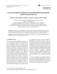
3. RESULTS AND DISCUSSION<br />
3.1 Thermal Analysis <strong>of</strong> Thermal Barrier<br />
Coating (TBC)<br />
The results <strong>of</strong> differential scanning calorimetry<br />
(DSC) and thermogravimetric analysis (TGA) <strong>of</strong><br />
YSZ top coat when exposed to 3.5% NaCl solution<br />
after 600 hours are shown in Fig. 1a & b, respectively.<br />
It was evaluated that loss in mass <strong>of</strong> coating when
Electrochemical Behavior <strong>of</strong> Yttria Stabilized Thermal Barrier Coating 237<br />
Fig. 1. Thermal analysis <strong>of</strong> TBC (a); DSC (b); TGA.<br />
<br />
<br />
behavior with continuous decrease in 0.5% weight<br />
in TGA was attributed to the stabilization <strong>of</strong> YSZ.<br />
<br />
was due to the dehydration process with about 0.2%<br />
weight loss which demonstrated the actual ability<br />
<strong>of</strong> physical absorption <strong>of</strong> water in the coating upto<br />
this temperature. The endothermic behavior <strong>of</strong> YSZ<br />
<br />
<br />
diffusion <strong>of</strong> anions (oxygen, chlorides) within the<br />
2<br />
after stabilization with Y 2<br />
3<br />
from the electrolyte. The addition <strong>of</strong> ‘Y ions’ in<br />
Zirconia occupies lattice positions which produce<br />
oxygen vacancies. With the addition <strong>of</strong> Yttria in<br />
Zirconia promote oxygen ions to ingress within the<br />
YSZ lattice (oxidation) with increase in temperature<br />
[10].<br />
coated sample. The potential at 0 hour was -594 mV<br />
and gradually increased to noble potential (-345.2<br />
mV) after 600 hours (Fig. 2). The tendency to shift<br />
potential in noble direction (positive direction) was<br />
<br />
coat surface but still active (-345.2 mV) potential<br />
was related to the presence <strong>of</strong> chloride ions in<br />
<br />
The shift <strong>of</strong> potential at the rate <strong>of</strong> 0.297 mV/hour<br />
towards noble direction indicated development <strong>of</strong><br />
<br />
3.2 Open Circuit Potential (OCP)<br />
The open circuit potential (E ocp<br />
) is a predictive<br />
parameter to estimate corrosion tendency <strong>of</strong> a<br />
system. The E ocp<br />
<strong>of</strong> TBC samples with respect<br />
to Saturated Calomel Electrode (SCE) was<br />
determined for 600 hours when immersed in 3.5%<br />
NaCl solution. The values <strong>of</strong> E ocp<br />
were determined<br />
after every 72 hours after initial stabilization for<br />
24 hours. The potential trend was extrapolated at 0<br />
hour to evaluate corrosion tendency <strong>of</strong> unexposed<br />
Fig. 2. <br />
time.<br />
3.3 Linear Polarization Resistance (LPR)<br />
<br />
corrosion rates and to understand kinetically
238 M. Farooq et al<br />
Fig. 3. Variation in Polarization Resistance (R p<br />
).<br />
controlled electrochemical reactions. The LPR<br />
<br />
and polarization resistance (R p<br />
) and current<br />
density (i d<br />
) values after each 72 hour interval were<br />
determined. The trend <strong>of</strong> change in R p<br />
value with<br />
time (Fig. 3). The increase in R p<br />
and decrease in i d<br />
values in 600 hours <strong>of</strong> exposure was observed and<br />
this tendency was considered due to the formation<br />
and accumulation <strong>of</strong> corrosion product within the<br />
pores <strong>of</strong> coating after 600 hours at the interface<br />
<strong>of</strong> top ceramic coat and bond coat. The initial R p<br />
and i d<br />
values after 24hours exposure were 21.80<br />
<br />
with respect to initial values reached to 46.31<br />
<br />
independence <strong>of</strong> Yittria stabalized Ziconia (YSZ)<br />
Fig. 4. Decrease in charge density measured by LPR.<br />
top coat to hinder the diffusion <strong>of</strong> electrolyte. The<br />
charge density <strong>of</strong> YSZ coating when immersed in<br />
3.5% NaCl solution was calculated by integrating<br />
the current potential values <strong>of</strong> LPR curves. It was<br />
deduced that initial charge density (160.6 µC/<br />
cm 2 ) <strong>of</strong> coating was deteriorated to 114.6 µC/cm 2<br />
as presented in Fig. 4. This decrease <strong>of</strong> 46 µC/<br />
cm 2 in charge density and increase in polarization<br />
resistance suggested the formation <strong>of</strong> corrosion<br />
product and accumulation within the pores in the<br />
coating after 600 hours exposure. This was also<br />
responsible for the reduction in the active sites for<br />
electrochemical reactions.<br />
3.4 Electrochemical Impedance Spectroscopy<br />
(EIS) <strong>of</strong> TBC<br />
The EIS Nyquist plots for coated samples were<br />
obtained at room temperature as shown in Fig.<br />
5. These plots were modeled and simulated with<br />
equivalent electrical circuit which was investigated<br />
<br />
95%. It was apparent from the EIS investigation that<br />
there were three time constants in the spectrums.<br />
The solution resistance and YSZ coating resistance<br />
at higher frequency and in the second time constant<br />
depicted kinetically controlled reactions at the<br />
interface <strong>of</strong> top coat and bond coat by developing<br />
<br />
<br />
hour. This decrease in R ct<br />
was due chloride ingress<br />
at the interface and localized reactions with oxide<br />
<br />
corrosion products. YSZ top coat resistance was very<br />
low due to free penetration <strong>of</strong> electrolyte through<br />
inherent micro-pores in the YSZ. The EIS study<br />
evaluated kinetic and mass transport controlled<br />
behavior <strong>of</strong> YSZ top coat and capacitative behavior<br />
<strong>of</strong> bond coat at low frequency in a third time constant<br />
was related with the formation <strong>of</strong> unstablized oxide<br />
<br />
<br />
interface <strong>of</strong> bond coat and top coat. This result for<br />
YSZ demonstrates typical behavior <strong>of</strong> TBC that<br />
mass transport controlled reactions transformed to<br />
kinetically controlled reactions at low frequency<br />
regime <strong>of</strong> impedance spectrum.
Electrochemical Behavior <strong>of</strong> Yttria Stabilized Thermal Barrier Coating 239<br />
Fig. 5. Electrochemical impedance spectroscopy (EIS) Nyquist plots.<br />
In TBC the kinetics <strong>of</strong> electrochemical reactions<br />
depend on the ionic resistance <strong>of</strong> electrolyte,<br />
<br />
thickness, porosity and intrinsic defects within the<br />
coating [7].<br />
4. CONCLUSIONS<br />
The thermal analysis <strong>of</strong> coating after exposure<br />
to 3.5% NaCl solution revealed the absorption<br />
<strong>of</strong> electrolyte within the coating and exothermic<br />
<br />
regime and a sharp dip for endothermic reactions<br />
corresponded to the stabilization <strong>of</strong> YSZ and<br />
dehydration <strong>of</strong> electrolyte, respectively. The initial<br />
loss in weight as revealed by thermal analysis was<br />
related to desorption <strong>of</strong> electrolyte while further<br />
increase in temperature and exothermic behavior<br />
<strong>of</strong> top coat and heat evolution corresponded to the<br />
stabilization <strong>of</strong> top coat. The shift <strong>of</strong> open circuit<br />
potential in positive direction and increase in<br />
polarization resistance with exposure time were<br />
<br />
<strong>of</strong> top and bond coat. But the decrease in charge<br />
transfer resistance (R ct<br />
) as determined by EIS was<br />
due chloride ingress at the interface and localized<br />
<br />
since their greater capability <strong>of</strong> hydrolyzing the<br />
corrosion product.<br />
5. REFERENCES<br />
1. Birks, N., G. H. Meier, & F. S. Pettit. Introduction<br />
to the High-Temperature Oxidation <strong>of</strong> Metals, 2nd<br />
ed. Cambridge University Press, Cambridge, UK<br />
(2006).<br />
2. Yu, Z., D.D. Hass, & H.N.G. Wadley. NiAl bond<br />
coats made by a directed vapor deposition approach.<br />
Materials Science and Engineering A 394: 43–52<br />
(2005).<br />
3. Zhou, Z. F., E. Chalkova, S.N. Lvov, P. Chou, & R.<br />
Pathania. Development <strong>of</strong> hydrothermal deposition<br />
process for applying Zirconia coating on BWR<br />
materials for IGSCC mitigation. Corrosion Science<br />
49 (2): 830–843 (2007).<br />
4. Podor, R., N. David, C. Rapin, M. Vilasi, & P.<br />
Berthod. Mechnism <strong>of</strong> corrosion layer formation<br />
during Zirconium immersion in (Fe) bearing glass<br />
melt. Corrosion Science 49 (8): 3226–3240 (2007).<br />
5. Wang, Z., A. Kulkarni, S. Deshpande, T. Nakamura,<br />
& H. Herman. Effect <strong>of</strong> pores and interfaces on<br />
effective properties <strong>of</strong> plasma sprayed Zirconia<br />
coatings. Acta Materialia 51: 5319–5334 (2003).<br />
6. Heung, R., X. Wang, & P. Xiao. Characterization <strong>of</strong><br />
<br />
impedance spectroscopy. Electrochimica Acta 5:<br />
1789-1793 (2006).<br />
7. Zhang, J., & V. Desai. Evaluation <strong>of</strong> thickness,<br />
porosity and pore shape <strong>of</strong> plasma sprayed TBC by<br />
electrochemical impedance spectroscopy. Surface<br />
Coatings Technology 190: 98-109 (2005).<br />
8. Byeon, J. W., B. Jayaraj, S. Vishweswaraiah, S.<br />
Rhee, V.H. Desai, & Y.H. Sohn. Non-destructive<br />
evaluation <strong>of</strong> degradation in multi-layered thermal<br />
barrier coatings by electrochemical impedance<br />
spectroscopy. Material Science and Engineering: A
240 M. Farooq et al<br />
407 (1-2): 213-225 (2005).<br />
9. Jayaraj, B., S.Vishweswaraiah,V.H.Desai, & Y.H.<br />
Sohn. Electrochemical impedance spectroscopy <strong>of</strong><br />
thermal barrier coatings as a function <strong>of</strong> isothermal<br />
and cyclic thermal exposure. Surface Coatings<br />
Technology 177–178: 140–151 (2004).<br />
10. American Ceramic Society. Progress in Thermal<br />
Barrier Coatings. John Wiley and Sons (2009).
Proceedings <strong>of</strong> the <strong>Pakistan</strong> <strong>Academy</strong> <strong>of</strong> <strong>Sciences</strong> 49 (4): 241–249 (2012) <strong>Pakistan</strong> <strong>Academy</strong> <strong>of</strong> <strong>Sciences</strong><br />
Copyright © <strong>Pakistan</strong> <strong>Academy</strong> <strong>of</strong> <strong>Sciences</strong><br />
ISSN: 0377 - 2969 print / 2306 - 1448 online<br />
Research Article<br />
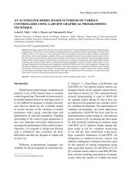
Agroclimatic Modelling for Estimation <strong>of</strong> Wheat Production<br />
in the Punjab Province, <strong>Pakistan</strong><br />
M. Jawed Iqbal 1,2* , Zaeem Uddin Ali 1 and S. Shahid Ali 3<br />
1<br />
Institute <strong>of</strong> Space and Planetary Astrophysics, University <strong>of</strong> Karachi, Karachi, <strong>Pakistan</strong><br />
2<br />
Department <strong>of</strong> Mathematics, University <strong>of</strong> Karachi, Karachi, <strong>Pakistan</strong><br />
3<br />
Department <strong>of</strong> Geography, University <strong>of</strong> Karachi, Karachi, <strong>Pakistan</strong><br />
Abstract: <strong>Pakistan</strong>’s economy hinges on agriculture and the most important agricultural commodity <strong>of</strong> the<br />
country is wheat. The province <strong>of</strong> Punjab has the predominant share in wheat production <strong>of</strong> the country.<br />
As agriculture sector is highly vulnerable to the climate change phenomena, the current global climatic<br />
<br />
<br />
article reports on an attempted agroclimatic model for the estimation <strong>of</strong> wheat production in Punjab using<br />
meteorological parameters.<br />
Keywords: Agroclimatic model, prediction <strong>of</strong> wheat yield, agrometeorological variables<br />
1. INTRODUCTION<br />
Agriculture is the linchpin <strong>of</strong> our national economy.<br />
According to economic survey <strong>of</strong> <strong>Pakistan</strong> 2011–<br />
2012 it has a share <strong>of</strong> 21% in the national GDP<br />
and employs 45% <strong>of</strong> the national labour force. The<br />
agricultural production system <strong>of</strong> <strong>Pakistan</strong> is based<br />
on irrigation. In <strong>Pakistan</strong> 84% <strong>of</strong> the total cultivated<br />
area (22.05 million ha) is under irrigation and the<br />
remaining is entirely rainfed or barani [1]. More<br />
than 90% <strong>of</strong> the available fresh-water resources in<br />
the country are utilized for irrigated agriculture [2].<br />
Punjab is <strong>Pakistan</strong>’s second largest province with<br />
205,344 km 2 (79,284 mi 2 ), after Balochistan, and<br />
is located at the northwestern edge <strong>of</strong> the<br />
geologic Indian plate in South Asia. The Fig. 1<br />
depicts the distribution <strong>of</strong> average yield <strong>of</strong> wheat<br />
in various districts across the country. According to<br />
McCarty’s measure, 28 out <strong>of</strong> 35 districts <strong>of</strong> Punjab<br />
have higher yield than the country’s average yield,<br />
i.e., 2.05 ton per hectare. The northern districts <strong>of</strong><br />
the Punjab have lower productivity per unit land<br />
area, primarily due to the topographical features<br />
and more relative humidity [3]. Several studies have<br />
highlighted agro-ecological zones for the growth<br />
————————————————<br />
Received, April 2012; Accepted, November 2012<br />
*Corresponding author, M. Jawed Iqbal; Email: javiqbal@uok.edu.pk<br />
and development <strong>of</strong> crops across the country [3, 4].<br />
The cultivate areas <strong>of</strong> the entire country are divided<br />
into 10 agro-ecological zones (Fig. 2). Out <strong>of</strong> which<br />
four agro-ecological zones, i.e., irrigated plains,<br />
Barani (rain fed) region, Thal region and Marginal<br />
Lands occur in the Punjab province.<br />
The agricultural sector <strong>of</strong> <strong>Pakistan</strong> is confronted<br />
with many problems. The provision <strong>of</strong> livelihood<br />
and food security for the fast growing population,<br />
without affecting the fragile ecosystem, are the<br />
main challenges to the agriculture sector. Being<br />
open to vagaries <strong>of</strong> nature, agriculture sector is<br />
highly susceptible to climate change phenomena.<br />
The scholars opine that human activities have<br />
reached a level where these are adversely affecting<br />
global environment. Anthropogenic perturbations<br />
are causing the global climate change at a much<br />
faster rate compared to natural pace. The current<br />
<br />
on sustainable agriculture production and food<br />
security as described by Adams et al. [5]. Increasing<br />
change in ambient temperature and rainfall and<br />
the resultant increased frequency and intensity <strong>of</strong>
242 M. Jawed Iqbal et al<br />
Fig. 1. Wheat growing areas in <strong>Pakistan</strong>, 2004-05 (courtesy: Dr. S.S. Ali).<br />
Fig. 2. Agro-ecological zones <strong>of</strong> Punjab (courtesy: Dr. S.S. Ali ).
Agroclimatic Modelling for Estimation <strong>of</strong> Wheat Production 243<br />
the crop-lands, pastures and forests. Thus, it was<br />
thought important to investigate the impact <strong>of</strong><br />
current climate change on agriculture <strong>of</strong> the country.<br />
Estimates <strong>of</strong> evapotranspiration <strong>of</strong>fer an outlook <strong>of</strong><br />
soil-water balance in association with the amount<br />
<br />
<br />
and irrigation scheduling [6]. Also, these estimates<br />
can help determine the nature <strong>of</strong> agro-climate,<br />
agro-climatic potential <strong>of</strong> the region and suitability<br />
<strong>of</strong> various crops or varieties which can be grown<br />
for obtaining the best economic returns [7].<br />
A recent study employed Growing Degree Days<br />
(GDD) for expressing the relationship between<br />
period <strong>of</strong> every plant growth phonological stage<br />
and the temperature degree [8]. Growing Degree<br />
Days <strong>of</strong> all Andhra Pradesh were correlated with<br />
variability <strong>of</strong> rice yield <strong>of</strong> this Indian state [9].<br />
Satellite-derived product <strong>of</strong> normalized difference<br />
vegetation index (NDVI) were used by Chakraborty<br />
et al. [10] for the estimation <strong>of</strong> rice yield. In this<br />
study as well, we employed NDVI for estimating<br />
the wheat yield <strong>of</strong> Punjab province by examining<br />
the relationship between wheat productivity per unit<br />
area and integrated NDVI. Finally, we constructed<br />
a multiple regression model <strong>of</strong> wheat in the Punjab<br />
using agro-meteorological variables derived from<br />
nearest stations, i.e., the remotely sensed satellite<br />
data (e.g. NDVI, GDD, and SOI).<br />
2. DATA AND METHODOLOGY<br />
2.1. Data<br />
Yield <strong>of</strong> wheat crop has been collected from website<br />
<strong>of</strong> Agriculture Marketing Information Service<br />
Directorate <strong>of</strong> Agriculture (Economics& Marketing)<br />
Punjab, Lahore. The <strong>Pakistan</strong> Meteorological<br />
Department provided data <strong>of</strong> daily maximum and<br />
minimum temperature <strong>of</strong> Lahore, Jhelum, Khanpur,<br />
Multan, Faisalabad, Islamabad, Bahawalpur, and<br />
annual data <strong>of</strong> rainfall <strong>of</strong> Islamabad, Jhelum, Lahore,<br />
Sargodha, Faisalabad, Multan, Bahawalpur.<br />
The following formula was used to compute the<br />
Growing Degree Days (GDD):<br />
where T max<br />
and T min<br />
are daily maximum and minimum<br />
temperature, T b<br />
is the threshold temperature below<br />
which growth <strong>of</strong> wheat crop is not possible, and<br />
T b<br />
<br />
<strong>of</strong> monthly GDD temperature for each mentioned<br />
stations using T max<br />
and T min<br />
. Next, the monthly data<br />
<strong>of</strong> GDD temperature <strong>of</strong> Punjab was computed by<br />
taking average <strong>of</strong> monthly GDD temperature for<br />
each mentioned stations.<br />
Normalized Difference Vegetation Index (NDVI)<br />
is the satellite-derived product which represents the<br />
green vegetation in area. It works on the phenomena<br />
that growing green plants absorb radiations in<br />
visible region and emit infra red radiation. Data <strong>of</strong><br />
NDVI can be downloaded from the website www.<br />
jisao.washington.edu. NVDI was computed using<br />
the formula:<br />
Where NIR<br />
R <br />
This spectral pattern is described by a value<br />
ranging from -1 (usually water) to +1 (strongly<br />
vegetative growth). We computed spatial average<br />
<strong>of</strong> monthly NVDI over the region <strong>of</strong> Punjab<br />
province.<br />
Other parameters which were used in this study<br />
is South Oscillation Index (SOI). SOI and Nino 3<br />
were obtained from the website www.cdc.noaa.<br />
gov. SOI was used to indicate El Nino and La Nina<br />
events. It is calculated by using the Mean Sea Level<br />
Pressure (MSLP) difference between Tahiti and<br />
Darwin. It can be calculated as:<br />
where P diff<br />
= (Average Tahiti MSLP for the<br />
month) - (Average Darwin<br />
MSLP for the month)<br />
P diffav<br />
= Long term average <strong>of</strong> P diff<br />
for<br />
the month<br />
SD (P diff<br />
) = Long term standard deviation<br />
<strong>of</strong> P diff<br />
for the month
244 M. Jawed Iqbal et al<br />
2.2. Methodology<br />
To examine the impact <strong>of</strong> agro-climatic parameters<br />
<br />
season mean <strong>of</strong> crops from November to April. It<br />
is important to understand the role <strong>of</strong> agro-climatic<br />
parameters in modelling for wheat crop. Albeit<br />
techniques for identifying parameters range from<br />
simple correlation analysis to advanced procedures<br />
such as canonical correlation and neural network<br />
[13, 14], we used the Pearson correlation analysis<br />
<br />
calculated between crop yields and agro-climatic<br />
parameters (e.g. rainfall, GDD, NVDI, SOI, etc.).<br />
Secondly, multiple linear regression equation<br />
was constructed between wheat yields <strong>of</strong> Punjab<br />
<br />
<br />
variance associated with each parameter designates<br />
the relative importance <strong>of</strong> the index in modulating<br />
the crop variability. Moreover, the total variance<br />
<br />
inter-annual variations. The linear regression model<br />
<br />
Y = b 0 + b i X i<br />
, (i {0, 1, 2, 3, ... ,p}),<br />
where Y is the estimated wheat yield in standardised<br />
unit, b 0 is the intercept, X i<br />
is a value <strong>of</strong> the i th<br />
predictor (agro-climatic parameter) in the model,<br />
b i is the model parameters representing the linear<br />
relationship between the predictor and predicted, p<br />
the number <strong>of</strong> the predictors variable in the model.<br />
3. RESULTS AND DISCUSSION<br />
Percentage departure <strong>of</strong> wheat yield in Punjab<br />
province from median 599.2 is plotted in Fig. 3.<br />
Percentage departure started from 65.5% and<br />
there is a fall initially up to minimum value <strong>of</strong><br />
132.2% (in 1952). After that it rose linearly with<br />
some ups and downs. It had the maximum value<br />
<strong>of</strong> 46.6% in the year 2006. Wheat yield was below<br />
the median till year 1977. Since 1978 the yield was<br />
above the median, except in 1983. In our study we<br />
also observed that during La Nina years (i.e., 1947,<br />
1948, 1949, 1954, 1955, 1956, 1964, 1967, 1970,<br />
1971, 1973, 1975, 1988, 1998, 2000, and 2007) the<br />
average yield <strong>of</strong> wheat was 558.32 kg/acre. During<br />
El-Nino Years (i.e., 1951, 1957, 1963, 1965, 1969,<br />
1972, 1976, 1982, 1986, 1987, 1991, 1997, 2002<br />
and 2009) the average yield was 621.68 kg/acre,<br />
which clearly indicated that warm phase <strong>of</strong> ENSO<br />
had positive effect on wheat yield. . Sarma et al [9]<br />
have also obtained similar results for rice production<br />
in Andhra Paradesh, a province <strong>of</strong> India.<br />
3.1 Variation in Wheat Yield with Meteorological<br />
Parameters<br />
<br />
increasing trend (Fig. 4). The annual rainfall and<br />
wheat crop yields are plotted in Fig. 5. It shows that<br />
the wheat yield increased linearly and its trend is<br />
<br />
linear from 1987 to 1998. But overall its trend did<br />
not described the variation in wheat yield. The<br />
highest wheat yield was recorded in the year 1999<br />
when the rainfall was observed 453 mm and the<br />
minimum wheat yield was recorded in the year 1983<br />
when the rainfall was 766 mm. Pearson correlation<br />
0.16,<br />
<br />
wheat area is irrigated by tube wells, this might be<br />
<br />
relationship <strong>of</strong> crop yield with the rainfall was also<br />
observed by Sarma et al [9].<br />
Fig. 6 depicts the plot <strong>of</strong> wheat yield with Nino<br />
Table 1.<br />
Parameters/Months Nov Dec Jan Feb Mar Apr Nov-Apr Selected Months<br />
SOI 0.38 * 0.36 * 0.12 0.30 0.25 0.14 0.28 0.38 * Nov-Dec<br />
GDD 0.45 ** 0.42 * -0.12 0.24 0.09 0.37 * 0.41 * 0.50 ** Nov-Dec<br />
NDVI -0.08 -0.29 0.40 * 0.58 *** 0.46 ** 0.03 0.22 0.52 ** Jan-Mar
Agroclimatic Modelling for Estimation <strong>of</strong> Wheat Production 245<br />
Fig. 3. Percentage departure <strong>of</strong> wheat yield in the Punjab.<br />
Fig. 4. Five-year moving average <strong>of</strong> wheat yield in the Punjab.<br />
Fig. 5. Variability <strong>of</strong> wheat yield with rainfall in the Punjab.
246 M. Jawed Iqbal et al<br />
3 SST. It was observed that there was no correlation<br />
between these variables; the Pearson correlation<br />
0.1, which was<br />
<br />
<br />
<br />
relation with Kharif crops whereas for Rabi crops<br />
it was not meaningful. There are different stages in<br />
growth <strong>of</strong> wheat plant. SOI has been tested month<br />
wise and its correlation with wheat yield which<br />
<br />
correlation (with p-value less than 0.1) during the<br />
months <strong>of</strong> November and December, we took the<br />
average <strong>of</strong> SOI for these two months for further<br />
analysis. This showed that the average SOI <strong>of</strong> the<br />
<br />
phonological stages <strong>of</strong> wheat plant growth. Fig. 7<br />
illustrates the variability <strong>of</strong> wheat yield with the<br />
Southern Oscillation index (during Nov-Dec).<br />
Southern Oscillation index varied from 2.69 in the<br />
ENSO year 1982 for wheat yield <strong>of</strong> 684 kg to 1.59<br />
in the ENSO year 1988 for wheat yield <strong>of</strong> 761.6<br />
kg.<br />
<br />
relationship with wheat yield in the months <strong>of</strong><br />
November and December. So we understand that<br />
GDD explain the initial development <strong>of</strong> wheat plant<br />
Fig. 6. Variability <strong>of</strong> wheat yield with Nino 3 SST in the Punjab.<br />
Fig. 7. Variability <strong>of</strong> wheat yield with SOI in the Punjab.
Agroclimatic Modelling for Estimation <strong>of</strong> Wheat Production 247<br />
growth. Wheat yield had linear dependency on GDD<br />
(Fig. 8). GDD had the range <strong>of</strong> 135 units with the<br />
lowest value <strong>of</strong> 646 units in the ENSO year 1997<br />
and highest value <strong>of</strong> 781 units in the year 1999 for<br />
the maximum yield <strong>of</strong> 1079 kg. It exhibited positive<br />
<br />
<br />
the period <strong>of</strong> January to March. Fig. 9 represents the<br />
proportionality <strong>of</strong> NDVI (for the months January<br />
to March) with wheat yield. Pearson correlation<br />
<br />
among all the other parameters. Its value was 0.52<br />
<br />
<strong>of</strong> NDVI was 0.79 in the ENSO year 1982 for wheat<br />
yield <strong>of</strong> 684 kg and the maximum value <strong>of</strong> NDVI<br />
was recorded in the year 1993, which was declared<br />
<br />
this year the wheat yield was 786.6 kg. It is relevant<br />
<br />
the model developed by Bazgeer et al [16] for the<br />
prediction <strong>of</strong> wheat yield <strong>of</strong> Hoshiarpur district <strong>of</strong><br />
Punjab, India.<br />
3.2 Statistical Model for Prediction <strong>of</strong> Wheat<br />
Yield<br />
<br />
meteorological parameters SOI (Nov-Dec), NDVI<br />
(Jan-Mar) and Growing Degree Day Temperature<br />
(Jan-Mar) for the Punjab province which (Table<br />
2). It shows that NDVI and GDD were mutually<br />
Fig. 9. Variability <strong>of</strong> wheat yield with NDVI in the Punjab.<br />
Fig. 10. A comparison <strong>of</strong> actual wheat yield with estimated wheat yield.
248 M. Jawed Iqbal et al<br />
Fig. 8. Variability <strong>of</strong> wheat yield with GDD in the Punjab.<br />
independent. The statistical model <strong>of</strong> wheat yield<br />
in the Punjab province for was constructed with<br />
two independent parameters (i.e. NDVI and GDD)<br />
by using multi-regression analysis. The regression<br />
equation was:<br />
Y = 587.54*X 1<br />
+1.34*X 2<br />
717.06<br />
where Y = Wheat Yield in kg/acre<br />
X 1<br />
= Seasonal average <strong>of</strong> NDVI <strong>of</strong><br />
Punjab for the months from<br />
January to March<br />
X 2<br />
= Seasonal average <strong>of</strong> Growing<br />
Degree Day Temperature <strong>of</strong><br />
Punjab for the months from<br />
November to December<br />
Table 2.<br />
Parameter NDVI GDD SOI<br />
NDVI 1.00 0.22 <br />
<br />
GDD 0.22 - <br />
<br />
SOI 0.20 0.41 * -<br />
<br />
<br />
model was +0.65. Thus, our model explained<br />
43% variability <strong>of</strong> wheat yield for the period from<br />
1980 to 2000. Fig. 10 shows the comparison <strong>of</strong><br />
actual wheat yield and estimated wheat yield. The<br />
maximum difference was approximately 190.82 kg<br />
in the year 2000 which was less than actual wheat<br />
yield.<br />
4. CONCLUSIONS<br />
This study demonstrated the impact <strong>of</strong> regional<br />
meteorological parameters (i.e., NDVI and SOI)<br />
<br />
wheat yield in Punjab province <strong>of</strong> <strong>Pakistan</strong>. The<br />
wheat yield was not dependant on rainfall; also<br />
Nino 3 SST had no explanation with regard to<br />
wheat productivity in the Punjab. However, South<br />
oscillation exhibited some relationship with wheat<br />
yield, but it was not included in the model because<br />
<br />
GDD temperature had greater impact on wheat<br />
yield. NDVI had a stronger correlation with wheat<br />
yield, compared to other parameters. Thus, we<br />
construct a multi-linear model for wheat yield by<br />
employing NDVI and GDD. This model explains<br />
the 43% variability <strong>of</strong> wheat yield for the 1980–<br />
2000 period.<br />
5. REFERENCES<br />
1. Iqbal, M. M., M. A. Goheer & A. M. Khan. Climate-<br />
Change Aspersion on Food Security <strong>of</strong> <strong>Pakistan</strong>.<br />
Science Vision 15(1): 15-23 (2009).<br />
2. Bhatti, M.A., and Akhtar. Increasing irrigated<br />
agricultural productivity for Poverty reduction<br />
in <strong>Pakistan</strong>. In: Second South Asia Water Forum,<br />
<strong>Pakistan</strong> Water Partnership, Vol. 2. 14-16 December<br />
2002, Islamabad, p. 600 (2002).<br />
3. Ali, S. S. Structure and Spatial Patterns <strong>of</strong><br />
Agriculture in <strong>Pakistan</strong>: A Study in Regionalization.<br />
PhD thesis, University <strong>of</strong> Karachi, Karachi, <strong>Pakistan</strong><br />
(2010).
Agroclimatic Modelling for Estimation <strong>of</strong> Wheat Production 249<br />
4. PARC. Agro-ecological Regions <strong>of</strong> <strong>Pakistan</strong>.<br />
<strong>Pakistan</strong> Agricultural Research Council, Islamabad<br />
(1980).<br />
5. Adams, R.M., B. H. S. Hurd, Lenhart, & N. Leary.<br />
Effects <strong>of</strong> global climate change on agriculture: an<br />
interpretative review. Climate Research 11: 19–30<br />
(1998).<br />
6. Rasul, G. Water requirement <strong>of</strong> wheat crop in<br />
<strong>Pakistan</strong>. J. <strong>of</strong> Engg. & App. Sci. 3(1): 65-79<br />
(1992).<br />
7. Rasul, G. & A. B. Farooqi. Water requirement <strong>of</strong><br />
cotton crop in <strong>Pakistan</strong>. J. <strong>of</strong> Engg. & App. Sci.<br />
4(2): 154-165 (1993).<br />
8. Esfandiary, F., G. Aghaie, & A. D. Mehr. Wheat<br />
Yield Prediction through Agro Meteorological<br />
Indices for Ardebil District. World <strong>Academy</strong> <strong>of</strong><br />
Science, Engineering and Technology 49: 32-35<br />
(2009).<br />
9. Sarma. A.A.L.N., T V. L. Kumar & K. Koteswararao.<br />
Development <strong>of</strong> an agroclimatic model for the<br />
estimation <strong>of</strong> rice yield. J. Ind. Geophys. Union 12<br />
(2): 89-96 (2008).<br />
10. Chakraborty, M., Panigraohy & J.S. Parihar. Use <strong>of</strong><br />
NOAA AVHRR data in cloud cover prone areas for<br />
rice yield and production estimation: A case study<br />
in Orissa state. Proc. Nat, Symp on Remote Sensing<br />
Applications for Resource Management with Special<br />
Emphasis on North East Region, Guwahati, Nov<br />
25-27, 1993, p. 285-291 (1993).<br />
11. Dubey, R. P., M. H. Kalubarme, O. P. Jhorar, & S.<br />
S. Cheema. Wheat yield models and production<br />
estimates for Patiala and Ludhiana districts based<br />
on Landsat – MSS and agro-meteorological data.<br />
<br />
Applications Center, Ahmadabad, p. 1-34 (1987).<br />
12. Sharma, A. R. K. Sood, & M. H.Kalubarme.<br />
Agrometeorological wheat yield forecast in<br />
Himachal Pradesh. J. Agromet. 6: 153-160 (2004).
Proceedings <strong>of</strong> the <strong>Pakistan</strong> <strong>Academy</strong> <strong>of</strong> <strong>Sciences</strong> 49 (4): 251–257 (2012) <strong>Pakistan</strong> <strong>Academy</strong> <strong>of</strong> <strong>Sciences</strong><br />
Copyright © <strong>Pakistan</strong> <strong>Academy</strong> <strong>of</strong> <strong>Sciences</strong><br />
ISSN: 0377 - 2969 print / 2306 - 1448 online<br />
Research Article<br />
MATLAB-based Sequence Analysis <strong>of</strong> muRdr1H, a Functionally<br />
Characterized Resistance Gene <strong>of</strong> Roses<br />
Aneela Yasmin 1 , Akhtar A. Jalbani 2 * and Abdul Samad Chandio 3<br />
1<br />
Department <strong>of</strong> Biotechnology, Faculty <strong>of</strong> Crop Production,<br />
Sindh Agriculture University, Tandojam-70060, <strong>Pakistan</strong><br />
2<br />
Information Technology Center, Sindh Agriculture University,<br />
Tandojam-70060, <strong>Pakistan</strong><br />
3<br />
Department <strong>of</strong> Irrigation and Drainage, Faculty <strong>of</strong> Agricultural Engineering,<br />
Sindh Agriculture University, Tandojam-70060, <strong>Pakistan</strong><br />
Abstract: One <strong>of</strong> the practical applications <strong>of</strong> Bioinformatics is sequence analysis through sequence<br />
<br />
<br />
s<strong>of</strong>twares available for the biological sequence alignment; in this paper some basic alignment algorithms are<br />
discussed and implemented in MATLAB Bioinformatics tool box. Two sequences analyzed by this tool box<br />
were muRdr1H and resistance protein <strong>of</strong> Populus trichocarpa (ACCESSION XP_002329162). muRdr1H is<br />
a functionally characterized member <strong>of</strong> Rdr1 resistance gene family <strong>of</strong> roses, active against black spot. The<br />
<br />
global sequence alignment. Our proposed work provides useful application <strong>of</strong> MATLAB which can help in<br />
interpretation and visualization <strong>of</strong> the data in molecular biology.<br />
Keywords: Sequence alignment, MATLAB, Bioinformatics, protein sequence<br />
1. INTRODUCTION<br />
Computer science in combination with biological<br />
science is a relatively new multidisciplinary area <strong>of</strong><br />
science, known as Bioinformatics. In this research<br />
area, Informatics involves the technology that<br />
uses computer for different purposes; for example,<br />
storage <strong>of</strong> biological data and for performing<br />
<br />
manipulation and distribution. As the data contains<br />
biological information, hence the distribution <strong>of</strong><br />
information is related to biological aspects, such<br />
as DNA, RNA and proteins [1]. In this domain,<br />
research focuses on the usage <strong>of</strong> computers because<br />
most <strong>of</strong> the tasks in genomics data analysis are<br />
highly repetitive. Moreover, the common activities<br />
performed in Bioinformatics research include<br />
mapping and analyzing or aligning DNA and protein<br />
sequences, comparing and creating 3-D models <strong>of</strong><br />
<br />
drug design and discovery.<br />
In computational biology the main aspects<br />
<strong>of</strong> using Informatics is to develop innovative<br />
algorithms to compute biological sequencerelated<br />
problems. In handling biological<br />
sequences, sequence alignment is a key process <strong>of</strong><br />
Bioinformatics and computational biology. During<br />
alignment, sequences are compared by identifying<br />
similar patterns and establishing residue-residue<br />
correspondence among related sequences [2, 3].<br />
Hence sequence alignment is a way <strong>of</strong> arranging<br />
primary sequences <strong>of</strong> DNA, RNA and proteins to<br />
detect similar regions that may be consequences <strong>of</strong><br />
————————————————<br />
Received, May 2012; Accepted, November 2012<br />
*Corresponding author, Akhtar A. Jalbani; Email: akjalbani@sau.edu.pk
252 Aneela Yasmin et al<br />
functional, structural or evolutionary relationship<br />
between the sequences. The resulting alignment<br />
produces revise transcript <strong>of</strong> mismatches, i.e.,<br />
insertions and deletions, where mismatches can<br />
be inferred as point mutations. As a result, we can<br />
infer how sequences with the identical origin would<br />
deviate from one another.<br />
Nowadays, new biological sequences are being<br />
generated at an exponential rate; hence sequence<br />
comparison is widely used in biological research to<br />
identify new proteins and can search for existing<br />
protein for drug or diseases discovery. In any<br />
genome project, newly determined sequences are<br />
<br />
in the genomic databases, such as NCBI, in order<br />
to discover similarities. As a result <strong>of</strong> comparison,<br />
one or more sequence alignments can be produced.<br />
Similarity score is one factor that can be associated<br />
with the sequence alignment. If new sequences are<br />
<br />
to the biological databases, like NCBI, ENTREZ<br />
(which integrates GenBank) [4]. These databanks<br />
are remotely accessible. Researchers take full<br />
advantages <strong>of</strong> these databases to query and compare<br />
their sequences using different Bioinformatics<br />
tools.<br />
<br />
expose the structural or functional importance <strong>of</strong><br />
unknown sequences. Here in this paper, two very<br />
important types <strong>of</strong> DNA alignments are discussed<br />
namely Global and Local alignment in MATLAB.<br />
MATLAB is a powerful tool for the modeling and<br />
simulation <strong>of</strong> various domains. It contains different<br />
toolbox for the different domain for example<br />
communication systems, image compression,<br />
Bioinformatics, etc. MATLAB provides tight<br />
integration <strong>of</strong> compiler and its simulating<br />
environment. In this paper, we focused on the<br />
Bioinformatics tool box, which contains different<br />
solutions for the biological research; sequence<br />
alignment is one <strong>of</strong> them. In local alignment, the<br />
assumption is made based on that the two sequences<br />
are not similar over entire length [5]. Hence it only<br />
<br />
similarities and the aligned two sequences show<br />
region based alignment without considering the<br />
alignment <strong>of</strong> the rest <strong>of</strong> the regions. It is possible<br />
that the two sequences to be aligned can be <strong>of</strong><br />
different lengths [6, 7] whereas global alignment<br />
uses dynamic programming to obtain global<br />
alignment between the two selected sequences.<br />
These two algorithms were applied in MATLAB.<br />
The two sequences selected to analyze in<br />
MATLAB were muRdr1H and TIR-NBS-<br />
LRR-resistance protein <strong>of</strong> Populus trichocarpa<br />
(ACCESSION XP_002329162). muRdr1H is a<br />
member <strong>of</strong> Rdr1 resistance gene family <strong>of</strong> roses<br />
active against black spot, a fungal disease. This gene<br />
<br />
active resistance genes against Dort E4, race 6 <strong>of</strong><br />
diplocarpon rosae [8, 9] whereas TIR-NBS-LRRresistance<br />
protein <strong>of</strong> Populus trichocarpa shares<br />
the highest identity (41%) to muRdr1H protein.<br />
It is important to state that the TIR-NBS-LRRresistance<br />
protein <strong>of</strong> Populus trichocarpa was not<br />
functionally characterized.<br />
2. MATERIALS AND METHODS<br />
To identify the homologues <strong>of</strong> muRdr1H gene<br />
BLASTx searches were carried out against the<br />
GeneBank non-redundant database (http://blast.<br />
ncbi.nlm.nih.gov). The selected two sequences were<br />
tested using MATLAB Bioinformatics s<strong>of</strong>tware<br />
tools (www.mathworks.com). Those two sequences<br />
are assumed to be identical in length. The sequence<br />
alignment is carried out from beginning to the end<br />
<br />
alignment. The two types <strong>of</strong> alignment methods<br />
considered for the practical assignment were local<br />
alignment and global alignment.<br />
2.1 Algorithms for the DNA Sequence<br />
Alignment<br />
DNA sequence strings consist <strong>of</strong> four alphabet<br />
letters (A, C, G, T) called nucleotides. The length<br />
<strong>of</strong> sequence is variable; hence algorithm should<br />
produce high quality sequence alignment from<br />
these four letters. In local alignment, we need to<br />
identify the isolated regions <strong>of</strong> high similarity from<br />
the entire DNA sequence that makes better choice<br />
in some situation for this type <strong>of</strong> alignment method<br />
but it is more complex in general [10].<br />
2.1.1. Local Alignment<br />
The local alignment is performed through very
MATLAB-based Sequence Analysis <strong>of</strong> muRdr1H 253<br />
well-known algorithm known as Smith-Waterman<br />
algorithm. It is used for determining identical regions<br />
between two nucleotides or proteins. The algorithm<br />
does not look for total sequence but it compares<br />
segments <strong>of</strong> all possible lengths and optimizes the<br />
similarity measures. Following steps should be<br />
considered for Smith-Waterman algorithm:<br />
Step-1: Fill all dynamic matrix<br />
<br />
max value and trace <strong>of</strong> max value for that patch<br />
which leads to the max value or score.<br />
The Smith-Waterman algorithm compares<br />
two DNA sequences based individual pair-wise<br />
comparison between the characteristics.<br />
2.1.2. Global Alignment<br />
Global alignment method uses dynamic<br />
programming, for this Needleman-Wunsch<br />
algorithm is the best algorithm for this type <strong>of</strong><br />
sequence alignment. From two sequences, this<br />
algorithm helps to identify the global alignment.<br />
This uses all elements <strong>of</strong> the two sequences for the<br />
alignment procedure. This is also called end-to-end<br />
alignment.<br />
All elements are considered in global sequence<br />
alignment method, therefore the scoring matrix will<br />
also become m*n (where m is the longer sequence<br />
and n is the shorter sequence). The optimal score<br />
can be calculated at each matrix position by adding<br />
current match score to last scored position and<br />
subtracting the gap penalties. Hence each matrix<br />
position may have +ve or –ve or even zero value.<br />
2.2. Sequence Alignment with MATLAB<br />
The algorithms discussed above can easily be<br />
<br />
best possible sequence alignment for nucleotide<br />
or protein. MATLAB contains different built-in<br />
functions to access the already stored sequencing<br />
data on the gene databanks. Using MATLAB we<br />
can apply global and local alignment method to<br />
<br />
entered by accession numbers <strong>of</strong> the sequences,<br />
sequences were retrieved in its Open Reading<br />
Frames (ORF). After bringing the information in<br />
MATLAB environment, we applied algorithms for<br />
comparison <strong>of</strong> sequences using global and local<br />
alignment with the score that determines the degree<br />
<strong>of</strong> similarity. At the end, Monte Carlo Techniques<br />
were applied in MATLAB environment to assess<br />
<br />
sequences were generated and their scores were<br />
<br />
statistics toolbox, the parameters <strong>of</strong> bar distribution<br />
were estimated and the probability density function<br />
<strong>of</strong> the estimated distribution was plotted in red line<br />
(Fig. 1).<br />
3. RESULTS AND DISCUSSION<br />
3.1. Selection <strong>of</strong> Sequences to Study Alignment<br />
Algorithms<br />
According to BLASTx searches muRdr1H protein<br />
shares the maximum, i.e., 41%, identity to TIR-NBS-<br />
LRR-resistance proteins <strong>of</strong> Populus trichocarpa<br />
(ACCESSION XP_002329162), both genes belong<br />
to the same class <strong>of</strong> TIR-NBS-LRR resistance<br />
genes, followed by 39-44% to hypothetical proteins<br />
<strong>of</strong> Vitis vinifera, 40% to TIR <strong>of</strong> Medicago truncatula<br />
(ACCESSION ABD28703), 40% to CMR1 <strong>of</strong><br />
Phaseolus vulgaris (ACCESSION ABH07384)<br />
and 39% identity to N-like protein <strong>of</strong> N. tabacum<br />
(ACCESSION BAF95888) for resistance to the<br />
Tobacco Mosaic Virus. Out <strong>of</strong> these sequences<br />
TIR-NBS-LRR-resistance proteins <strong>of</strong> Populus<br />
trichocarpa was selected for the alignment with<br />
muRdr1H using MATLAB to demonstrate the<br />
utility <strong>of</strong> this s<strong>of</strong>tware for searching differences in<br />
their protein sequences.<br />
3.2. Open Reading Frame <strong>of</strong> Selected Sequences<br />
in MATLAB Environment<br />
The protein sequences <strong>of</strong> both genes were in text<br />
format. We used the same sequence by using<br />
seqshoworfs MATLAB method to open it in open<br />
reading frame work reader (ORF) as shown in Fig.<br />
2.<br />
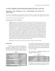
3.3. Dot Plot based Comparison in MATLAB<br />
Environment<br />
The dot plot representation <strong>of</strong> selected sequences<br />
is shown in Fig. 3. This basic sequence alignment<br />
method compares two sequences in graphical<br />
method by comparing two dimensional matrix; two<br />
sequences are written in vertical and horizontal
254 Aneela Yasmin et al<br />
Fig. 1. muRdr1H and TIR-NBS-LRR resistance<br />
protein <strong>of</strong> Populus trichocarpa are assessed using Monte Carlo Techniques.<br />
Fig. 2. Open Reading Framework (ORF) options for muRdr1H Sequence in MATLAB.
MATLAB-based Sequence Analysis <strong>of</strong> muRdr1H 255<br />
Fig. 3. Dot plot <strong>of</strong> muRdr1H and TIR-NBS-LRR resistance protein <strong>of</strong> Populus trichocarpa in MATLAB<br />
environment.<br />
Fig. 4. Global Alignment <strong>of</strong> muRdr1H and TIR-NBS-LRR resistance protein <strong>of</strong> Populus<br />
trichocarpa.
256 Aneela Yasmin et al<br />
Fig. 5. Local Alignment <strong>of</strong> <strong>of</strong> muRdr1H and TIR-NBS-LRR resistance protein <strong>of</strong> Populus trichocarpa.<br />
axes <strong>of</strong> the matrix and compared [10]. The selected<br />
sequences exhibited substantial regions <strong>of</strong> similarity<br />
(Fig. 3). Many dots are lined up in a diagonal line<br />
revealing some sequence alignment that will be<br />
<br />
and global alignment. It is obvious from the line that<br />
TIR and NBS region <strong>of</strong> protein has more similarity<br />
as compared to the end region that represents LRR<br />
<br />
both proteins, which was 41% as described above.<br />
3.4. Global and Local Sequence Alignments<br />
Both sequences are compared using global and local<br />
alignment methods. For global alignment we used<br />
Needle-Wunsch algorithm in the MATLAB and the<br />
resultant aligned global sequence is shown in Fig<br />
3. The scoring <strong>of</strong> global alignment is 749.33 with<br />
522/ 1232 (42%) identities and 822/ 1232 (67%)<br />
positives. The same sequences were used for local<br />
alignment. In which we used Smith-Waterman<br />
algorithm, where pair wise comparison is shown<br />
<br />
is 766.66 with 43% identities and 67% positives.<br />
Sequences with good similarity did not show much<br />
difference between local and global alignments.<br />
<br />
conserved regions <strong>of</strong> a gene.<br />
The number <strong>of</strong> identities and positives in global<br />
and local alignments are shown in Fig. 4 and Fig.<br />
5, respectively. Actually this did not represent the<br />
<br />
Techniques in MATLAB environment to assess<br />
<br />
methods. The random sequences were generated in<br />
MATLAB and their scores were plotted as bars (Fig<br />
<br />
gave the scores <strong>of</strong> 49.28 and 9.5. The probability<br />
density function <strong>of</strong> the estimated distribution was<br />
plotted which clearly showed that global alignment
MATLAB-based Sequence Analysis <strong>of</strong> muRdr1H 257<br />
In this paper, global and local alignment<br />
algorithms were developed and simulated using<br />
MATLAB. For global alignment, Needleman-<br />
Wunsch algorithm and for local alignment Smith-<br />
Waterman algorithm were used in MATLAB. This<br />
demonstration <strong>of</strong> data mining, visualization and <strong>of</strong><br />
course interpretation in MATLAB can facilitate the<br />
sequence data handling in molecular biology.<br />
4. REFERENCES<br />
1. Mathkour, H. & M. Ahmad. A comprehensive<br />
survey on genome sequence analysis. In: IEEE<br />
International Conference on Bioinformatics and<br />
Biomedical Technology, p. 14-18 (2010).<br />
2. Benkrid, K., Y. Liu & A. Benkrid. A highly<br />
<br />
for pairwise biological sequence alignment. IEEE<br />
Transactions on Very Large Scale Integration<br />
Systems 17(4): 561-570 (2009).<br />
3. Boukerche, A., J. M. Correa, A. Cristina M.A de<br />
Melo & R. P. Jacob. A hardware accelerator for<br />
the fast retrieval <strong>of</strong> DIALIGN biological sequence<br />
alignments in linear space. IEEE Transactions on<br />
Computers 59(6): 808-821 (2010).<br />
<br />
<br />
sequence alignment. IEEE/ACM Transactions on<br />
Computational Biology and Bioinformatics 6(4):<br />
570-562 (2009).<br />
5. Nguyen, V., A. Cornu & D. Lavenier. Implementing<br />
protein seed-based comparison algorithm on the<br />
SGI RASC-100 platform. In: IEEE Symposium on<br />
Parallel and Distributed Processing. p. 1-7 (2009).<br />
6. Bandyopadhayay, S. & R. Mitra. A parallel<br />
pairwise local sequence alignment algorithm. IEEE<br />
Transactions on Nano Bioscience 8(2): 139-146<br />
(2009).<br />
7. Nahar, N., M. Popstova & J. Gogarten. GPX: A tool<br />
for the exploration and visualization <strong>of</strong> genome<br />
evolution. In: 7th IEEE International Conference on<br />
Bioinformatics and Bioengineering, p. 1338-1342<br />
(2007).<br />
8. Yasmin, A. <br />
Characterization <strong>of</strong> Rdr1 Resistance Gene from<br />
Roses. PhD thesis, University <strong>of</strong> Hannover, Germany<br />
(2010).<br />
9. Terefe-Ayana, D., A. Yasmin, T. L. Le, H. Kaufmann,<br />
A. Biber, A. Kuehr, M. Linde & T. Debener. Mining<br />
disease resistance genes in roses: functional and<br />
molecular characterization <strong>of</strong> the Rdr1 locus.<br />
Frontiors <strong>of</strong> Plant Science 2:35, doi: 10.3389/<br />
fpls.2011.00035 (2011).<br />
10. Mai, S. M., M. Hamdy, M. Aboelfotoh & Y. M.<br />
Kadah. BIOINFTool: Bioinformatics and sequence<br />
data analysis in molecular biology using MATLAB.<br />
In: Cairo International Biomedical Engineering<br />
Conference, p. 1-9 (2006).
Proceedings <strong>of</strong> the <strong>Pakistan</strong> <strong>Academy</strong> <strong>of</strong> <strong>Sciences</strong> 49 (4): 259–267 (2012) <strong>Pakistan</strong> <strong>Academy</strong> <strong>of</strong> <strong>Sciences</strong><br />
Copyright © <strong>Pakistan</strong> <strong>Academy</strong> <strong>of</strong> <strong>Sciences</strong><br />
ISSN: 0377 - 2969 print / 2306 - 1448 online<br />
Original Article<br />
Comparative Sequence Analysis <strong>of</strong> Some Rdr1 Resistance Genes<br />
from <br />
Aneela Yasmin 1 , Akhtar A. Jalbani 2 * and Thomas Debener<br />
1<br />
Department <strong>of</strong> Biotechnology, Sindh Agriculture University, Tandojam, <strong>Pakistan</strong><br />
2<br />
Information Technology Center, Sindh Agriculture University, Tandojam, <strong>Pakistan</strong><br />
3<br />
Institute <strong>of</strong> Plant Genetics, University <strong>of</strong> Hannover, D-3419, Hannover, Germany<br />
Abstract: Rdr1 <br />
active against a fungal disease, black spot, <strong>of</strong> roses. Rdr1 locus consists <strong>of</strong> nine genes named as muRdr1A<br />
to muRdr1I. Functional and molecular characterization <strong>of</strong> this locus, revealed the presence <strong>of</strong> one gene,<br />
muRdr1H, active against Dort E4, race 6 <strong>of</strong> Diplocarpon rosae. In the present study we aimed to analyze<br />
the protein sequences <strong>of</strong> three members <strong>of</strong> this Rdr1 gene family for their homologies, important domains,<br />
conserved regions and selection pressure to get insights <strong>of</strong> their functionality based on protein sequence.<br />
The protein sequences <strong>of</strong> one active gene, muRdr1H and two inactive genes, muRdr1C and muRdr1G, were<br />
deduced and dissected using internet based bioinformatics tools. All three proteins belong to the TIR-NBS-<br />
LRR family <strong>of</strong> resistance genes. Although these proteins carry all necessary domains and conserved regions<br />
necessary for the functionality <strong>of</strong> TIR-NBS-LRR proteins, LRR region <strong>of</strong> the proteins, found under selection<br />
<br />
Keywords: Rdr1, rose, black spot, TIR-NBS-LRR proteins, resistance genes<br />
1. INTRODUCTION<br />
The most devastating fungal diseases <strong>of</strong> roses are<br />
powdery mildew, black spot and downy mildew.<br />
Powdery mildew usually infects roses grown in<br />
greenhouses whereas the black spot is a problem<br />
<br />
moist conditions throughout the world [1]. The<br />
present control <strong>of</strong> this disease is fungicidal sprays.<br />
On the other hand use <strong>of</strong> resistant varieties with<br />
durable genetic resistance is the safest option for<br />
the sustainable environment. Most <strong>of</strong> the cultivated<br />
roses lack natural resistance against black spot<br />
thus it has to be introgressed from wild roses [2].<br />
Nevertheless the exploitation <strong>of</strong> natural genetic<br />
resistance requires understanding <strong>of</strong> the resistance<br />
genes in terms <strong>of</strong> diversity, genomic organization<br />
and functionality.<br />
Rdr1 <br />
resistance gene locus found active against black<br />
spot (Diplocarpon rosae) <strong>of</strong> roses through<br />
phytopathological methods [3]. This Rdr1 locus<br />
was later mapped to a telomeric position <strong>of</strong> linkage<br />
group 1 in the diploid population 94/1 [4]. The<br />
construction <strong>of</strong> two large insert BAC libraries [5,<br />
<br />
location <strong>of</strong> Rdr1 gene within a 220 kb region [6].<br />
The 220 kb region contains 9 copies <strong>of</strong> “resistancegene-analogues”<br />
sequences (RGA) <strong>of</strong> the T1R-<br />
NBS-LRR type <strong>of</strong> resistance genes [7]. Out <strong>of</strong> these<br />
9 genes one gene muRdr1H was found as major<br />
active gene against Dort E4, race-6 <strong>of</strong> Diplocarpon<br />
rosae by functional characterization [8, 9].<br />
In TIR-NBS-LRR resistance genes, TIR motif<br />
is similar to toll/interleukin-1-receptor (TIR),<br />
the NBS is a part <strong>of</strong> a nucleotide binding (NB)-<br />
ARC domain that belongs to the STAND (signal<br />
transduction ATPases with numerous domains)<br />
family <strong>of</strong> NTPases. These proteins are proposed<br />
————————————————<br />
Received, May 2012; Accepted November 2012<br />
*Corresponding author: Akhtar A. Jalbani; Email: akjalbani@sau.edu.pk
260 Aneela Yasmin et al<br />
to regulate signal transduction as NB domain<br />
hydrolyzes NTP and changes its conformational<br />
states [10]. The NB-ARC domain has three subdomains<br />
conserved in NBS-LRR proteins: a P-loop<br />
<br />
<br />
bundle, and an ARC2 adopting a winged-helix fold<br />
that is connected to the LRR domain by a short<br />
linker [10]. LRR domains contain various numbers<br />
<strong>of</strong> tandemly repeated leucine-rich motifs with a<br />
conserved core consensus <strong>of</strong> L-X-X-L-X-L-X-X-N<br />
<br />
structure <strong>of</strong> the LRR domain suggests its role in<br />
different intra and intermolecular interactions <strong>of</strong><br />
direct recognition <strong>of</strong> pathogen effectors, regulating<br />
protein activation and signal transduction [12].<br />
The current research was aimed to analyze protein<br />
sequences <strong>of</strong> three paralogs <strong>of</strong> Rdr1 locus namely<br />
muRdr1H (AEE43932), muRdr1C (AEE43927) and<br />
muRdr1G (AEE43931). These paralogs are unique<br />
in a sense that these are the only members <strong>of</strong> this<br />
family for which 3’ and 5’ RACE products are<br />
available and are functionally characterized against<br />
Dort.E4. In this study we tried to get an insight in<br />
protein functionality based on their sequences and<br />
evaluated the selection pressure exerted on the genes.<br />
For this sequence variability, nucleotide substitution<br />
rates and amino acid homology check were carried<br />
out using different bioinformatics tools.<br />
2. MATERIAL AND METHODS<br />
<br />
technique was used to obtain the 5’ and 3’ ends <strong>of</strong><br />
RNA transcripts <strong>of</strong> muRdr1C, G and H transiently<br />
expressed in tobacco [8, 9]. Isolated and sequenced<br />
RACE products were used to get cDNA sequence<br />
from previously sequenced BAC clones [6, 9].<br />
Protein sequences <strong>of</strong> three proteins were obtained<br />
using full length cDNA [8] in S<strong>of</strong>t-ware Bioedit<br />
Version 7.0.9 [13].The same s<strong>of</strong>tware was used for<br />
the protein sequence editing, alignment, multiple<br />
alignment (ClustalW) and local BLAST searches to<br />
analyze and obtain conserved regions. Nucleotide<br />
sequence <strong>of</strong> muRdr1H (cDNA) was used for Blastx<br />
searches (http://www.ncbi.nlm.nih.gov/blast/<br />
<br />
proteins to muRdr1H. For Neignbor-joining (NJ)<br />
analysis the homologous protein sequences were<br />
downloaded from NCBI database and phylogenetic<br />
tree was constructed in MEGA4 [14, 15]. The gene<br />
prediction and protein analysis were performed<br />
on different free internet sources as http://www.<br />
expasy.ch/, http://swissmodel.expasy.org/SWISS-<br />
MODEL. html, http://www.ebi.ac.uk/interpro/,http://<br />
linux1.s<strong>of</strong>tberry.com/berry.phtml whereas the<br />
ratio <strong>of</strong> synonymous (K s<br />
) and non-synonymous<br />
(K a<br />
) substitutions rates per synonymous/ nonsynonymous<br />
site were calculated using s<strong>of</strong>tware<br />
DnaSP v 5 [16].<br />
3. RESULTS AND DISCUSSION<br />
Rdr1 resistance locus in consists <strong>of</strong><br />
a cluster <strong>of</strong> nine paralogs disease resistance genes<br />
that play important roles in innate immunity against<br />
black spot. The protein sequences <strong>of</strong> three members,<br />
muRdr1C, muRdr1H and muRdr1G, were deduced<br />
and subjected to sequence variability, nucleotide<br />
substitution rates and amino acid homology check.<br />
According to previous studies, among the nine R<br />
genes in this locus muRdr1H confers partial resistance<br />
to race 6 <strong>of</strong> the fungal pathogen Diplocarpon rosae<br />
[8, 9, 17]. The muRdr1H transcript resulted in the<br />
Open Reading Frame (ORF) <strong>of</strong> 1122 amino acids<br />
muRdr1C has the predicted<br />
protein <strong>of</strong> 1139 aa whereas the deduced protein <strong>of</strong><br />
muRdr1G has 944 amino acids. All three proteins<br />
show the presence <strong>of</strong> TIR, NBS and LRR domains<br />
with all conserved motifs as suggested by Lukasik<br />
and Takken [18] and Meyers and colleagues [19]<br />
(Fig. 1).<br />
The homologues <strong>of</strong> muRdr1H protein were<br />
<br />
out against the GenBank non-redundant database<br />
(http://blast.ncbi.nlm.nih.gov). The muRdr1H<br />
protein shares the highest identity (41%) to TIR-<br />
NBS-LRR-resistance protein <strong>of</strong> Populus trichocarpa<br />
(ACCESSION XP_002329162). It also shows<br />
identity to hypothetical proteins <strong>of</strong> Vitis vinifera<br />
(39-44%), to TIR <strong>of</strong> Medicago truncatula (40%;<br />
ACCESSION ABD28703), to CMR1 <strong>of</strong> Phaseolus<br />
vulgaris (40%; ACCESSION ABH07384) and to<br />
N-like protein <strong>of</strong> N. tabacum (39%; ACCESSION<br />
BAF95888 for resistance to Tobacco Mosaic Virus).<br />
Fig. 2 shows phylogenetic tree <strong>of</strong> different amino
261
262 Aneela Yasmin et al<br />
Fig. 1. Alignment <strong>of</strong> the proteins <strong>of</strong> muRdr1H, C and G <strong>of</strong> roses, TIR-NBS-LRR resistance protein<br />
<strong>of</strong> Populus trichocarpa and N like protein <strong>of</strong> N. tabacum. The muRdr1H protein and its predicted<br />
TIR, NBS and LRR domains with conserved motifs are under-lined. Stars on muRdr1H protein sequence<br />
represent unique amino acids <strong>of</strong> this protein when compared to proteins <strong>of</strong> muRdr1C and G.<br />
Within muRdr1H protein sequence the end amino acid <strong>of</strong> each domain is marked bold. a- Numbers in<br />
muRdr1H (1), muRdr1C (2), muRdr1G (3), resistance protein <strong>of</strong> Populus<br />
trichocarpa (4) and N like protein <strong>of</strong> N. tabacum (5); b and c- sequence positions; dashes indicate gaps<br />
inserted to maintain optimal alignment.<br />
acid sequences showing considerable identity to<br />
muRdr1H protein, these full length aligned protein<br />
sequences were downloaded from NCBI and tree<br />
was constructed based on the bootstrap neignborjoining<br />
(NJ) method with the Kimura2-parameter<br />
model by MEGA4 [14, 15]. It is interesting to code<br />
here that the CMR1 is a viral resistance gene from<br />
common bean that functions across plant families<br />
[20]. This protein sequence shows 40% identity<br />
to the muRdr1H protein that found to be active<br />
against black spot fungus, which suggests that the<br />
predicted NB-LRR structures and recognition <strong>of</strong><br />
certain pathogen type lack correlation.<br />
The kind <strong>of</strong> selection pressure exerted on different<br />
domains <strong>of</strong> the genes was estimated by calculating<br />
ratio <strong>of</strong> synonymous (K s<br />
) and non-synonymous<br />
(K a<br />
) rates <strong>of</strong> substitutions for each synonymous/<br />
non-synonymous site <strong>of</strong> different parts <strong>of</strong> the ORF<br />
<strong>of</strong> three paralogs (muRdr1H, G and C). When K a<br />
/ K s<br />
ratio is 1 it represents random mutation or no<br />
selection pressure operating on sequences may be<br />
K a<br />
/ K s<br />
> 1) or conservation <strong>of</strong><br />
sequence (K a<br />
/ K s<br />
< 1) [21]. Estimation <strong>of</strong> the number<br />
<strong>of</strong> synonyms and non-synonyms nucleotide per site
263<br />
Fig. 2. NJ analysis <strong>of</strong> protein sequence showing considerable similarities to<br />
muRdr1H. The full length aligned protein sequences were downloaded from NCBI<br />
and analyzed in MEGA 4.0.<br />
showed that the three genes are under conservation<br />
selection and all domains (TIR, NBS and LRR<br />
domain) are not under positive selection compared<br />
<br />
motifs which showed K a<br />
/ K s<br />
ratio > 1 (Table 1). The<br />
comparison <strong>of</strong> complete LRR domains <strong>of</strong> muRdr1H<br />
and muRdr1C resulted in higher K a<br />
values than K s<br />
<br />
<br />
actually the result <strong>of</strong> lower K s<br />
for the N- and C-<br />
<br />
shows a K a<br />
/ K s<br />
>1 (Table 1). Although three genes<br />
show conserved type <strong>of</strong> selection, LRR domains<br />
show the highest frequency <strong>of</strong> non-synonymous<br />
substitutions followed by NBS domain. The K a<br />
/ K s<br />
ratios were calculated for C-terminal region<br />
<br />
in this region. This supported the hypothesis that<br />
the parts <strong>of</strong> proteins which participate in pathogen<br />
recognition are under diversifying selection. This<br />
pattern is in agreement to previous studies that show<br />
diversifying selection acts on the LRR encoding<br />
domain <strong>of</strong> various plant disease resistance genes<br />
[11].<br />
Comparison <strong>of</strong> muRdr1H protein sequence with<br />
other two (muRdr1C and muRdr1G) members<br />
<strong>of</strong> the same Rdr1 family revealed 119 muRdr1H<br />
<br />
which are part <strong>of</strong> TIR (2 aa; 0.002%), NBS (40 aa;<br />
3.6%), and LRR (77 aa; 6.8%) domains (Fig. 3).<br />
For RAG8, as the majority <strong>of</strong> unique amino acids<br />
are located in LRR region followed by NBS region<br />
suggesting some important role <strong>of</strong> these domains<br />
in functionality <strong>of</strong> muRdr1H. The deduced Gro1-4<br />
protein (resistance gene) showed only 16 nonconserved<br />
differences in amino acids sequence
264 Aneela Yasmin et al<br />
Fig. 3. Comparison <strong>of</strong> protein sequences encoded by 3-members <strong>of</strong> Rdr1 family. Protein sequences<br />
muRdr1H (1), muRdr1C (2) and muRdr1G (3) were aligned to check amino acid similarities<br />
and divergence. Stars represent consensus sequence and dots show differences in amino acids. a-<br />
muRdr1H, G & C proteins sequences; b and c- sequence positions; dashes indicate gaps inserted<br />
to maintain optimal alignment.
265<br />
Table 1. Sequence variability and nucleotide diversity in different regions <strong>of</strong> three paralogs <strong>of</strong> Rdr1<br />
family.<br />
aa 2 (%) K a<br />
K s<br />
K a<br />
/ K s<br />
R-genes compared Analyzed regions 1 Nucleotide substitutions 3<br />
muRdr1H vs.<br />
muRdr1C<br />
Complete CDS<br />
80 0.0977 0.1041 0.92<br />
TIR domain<br />
90 0.0484 0.0836 0.58<br />
NBS domain<br />
76<br />
0.1168<br />
0.1196<br />
0.98<br />
Complete LRR domain<br />
79<br />
0.1034<br />
0.0983*<br />
1.05<br />
<br />
-<br />
0.1146<br />
0.1108<br />
1.03<br />
xxLxLxx motif<br />
-<br />
0.0722<br />
0.0935<br />
0.77<br />
muRdr1H vs.<br />
muRdr1G<br />
<br />
Complete CDS<br />
TIR domain<br />
-<br />
75<br />
98<br />
0.1679<br />
0.0991<br />
0.0079<br />
0.1156<br />
0.1354<br />
0.0356<br />
1.45<br />
0.73<br />
0.22<br />
NBS domain<br />
78<br />
0.1184<br />
0.1853<br />
0.64<br />
Complete LRR domain<br />
66<br />
0.1209<br />
0.1429<br />
0.85<br />
<br />
-<br />
0.1148<br />
0.0530<br />
2.17<br />
xxLxLxx motif<br />
-<br />
0.0717<br />
0.1142<br />
0.63<br />
muRdr1G vs.<br />
muRdr1C<br />
<br />
Complete CDS<br />
TIR domain<br />
-<br />
64<br />
90<br />
0.5067<br />
0.1180<br />
0.0512<br />
0.5738<br />
0.1497<br />
0.1134<br />
0.88<br />
0.79<br />
0.45<br />
NBS domain<br />
71<br />
0.1439<br />
0.1737<br />
0.83<br />
Complete LRR domain<br />
52<br />
0.1267<br />
0.1508<br />
0.84<br />
<br />
-<br />
0.0740<br />
0.1132<br />
0.65<br />
xxLxLxx motif<br />
-<br />
0.0793<br />
0.1249<br />
0.64<br />
muRdr1H vs.<br />
muRdr1G &C<br />
<br />
Complete CDS<br />
TIR domain<br />
-<br />
58<br />
89<br />
0.5657<br />
0.09228<br />
0.02736<br />
0.5029<br />
0.11032<br />
0.05688<br />
1.13<br />
0.83<br />
0.47<br />
NBS domain<br />
67<br />
0.10896<br />
0.13689<br />
0.78<br />
Complete LRR domain<br />
49<br />
0.10421<br />
0.11089<br />
0.94<br />
<br />
-<br />
0.10613<br />
0.07759<br />
1.40<br />
xxLxLxx motif<br />
-<br />
0.06861<br />
0.09678<br />
0.69<br />
<br />
-<br />
0.25922<br />
0.25760<br />
1.01<br />
1<br />
Different region <strong>of</strong> R-genes is analyzed for nucleotide variability.<br />
2<br />
Amino acid (aa) homology in percentage.<br />
3<br />
The ratio <strong>of</strong> synonymous (K s<br />
) and non-synonymous (K a<br />
) substitutions rates per synonymous/ non-synonymous site were calculated using s<strong>of</strong>tware<br />
DnaSP v 5.<br />
*<br />
Under-lined numbers represent the exceeded value <strong>of</strong> synonymous (K s<br />
) compared to non-synonymous (K a
266 Aneela Yasmin et al<br />
when compared to non-functional members <strong>of</strong> the<br />
Gro1 gene family [22]. Mutagenesis analysis <strong>of</strong><br />
the muRdr1H protein or comparison <strong>of</strong> functional<br />
and non-functional orthologs could determine<br />
the essential residues necessary for pathogen<br />
recognition and/ or downstream signaling. The Rdr1<br />
<br />
D. rosae [23]. It is possible that the other members<br />
<strong>of</strong> this family are also functionally active against<br />
other races <strong>of</strong> D. rosae. Although the amino acid<br />
sequence identity <strong>of</strong> these three paralogs <strong>of</strong> Rdr1<br />
resistance gene cluster ranges between 58% and<br />
80% and muRdr1H shares the highest overall amino<br />
acid sequence homology to muRdr1C (80%; Table<br />
1) the functionality <strong>of</strong> muRdr1C and muRdr1G<br />
should be explored against different isolates <strong>of</strong> D.<br />
rosae and/ or some other taxonomically different<br />
pathogens.<br />
Alignment <strong>of</strong> deduced amino acids <strong>of</strong> muRdr1H,<br />
C and G show that the higher degree <strong>of</strong> sequence<br />
similarity is present in N-terminal halves <strong>of</strong><br />
proteins that harbour putative effector domains<br />
when compared to the C-terminal halves <strong>of</strong><br />
proteins (Fig. 3) suggesting the LRR domain under<br />
selection as demonstrated for other closely related<br />
NBS-LRR proteins [24]. This kind <strong>of</strong> selection in<br />
LRR domain is exerted by single base changes,<br />
insertions, deletions and unequal exchange <strong>of</strong><br />
meiotic recombination events for the evolution<br />
<br />
between closely linked R-genes in a cluster [25].<br />
4. CONCLUSION<br />
The functionally characterized muRdr1H which<br />
was found active against Dort E4 and other two<br />
sequences has all conserved regions <strong>of</strong> TIR-NBS-<br />
LRR genes. muRdr1G and C were inactive when<br />
challenged by Dort E4. Due to the homology <strong>of</strong> two<br />
paralogs to muRdr1H, we suggest their functional<br />
characterization against other races <strong>of</strong> D. rosae to<br />
assess their functionality on molecular level. We<br />
observed less selection pressure exerted on these<br />
genes as the pathogen D. rosae has low mobility<br />
and races.<br />
5. REFERENCES<br />
1. Horst, R. K. Compendium <strong>of</strong> Rose Diseases. The<br />
American Phytopathological Society, St.Paul,<br />
Minn., p. 7–11 (1983).<br />
2. Schulz, D. F., M. Linde, O. Blechert & T. Debener.<br />
Evaluation <strong>of</strong> genus Rosa germplasm for resistance<br />
to black spot, downy mildew and powdery mildew.<br />
European <strong>Journal</strong> <strong>of</strong> Horticulture <strong>Sciences</strong> 74 (1):<br />
1–9 (2009).<br />
3. Debener, T., R. Drewes-Alvarez & K. Rockstroh.<br />
<br />
spot, Diplocarpon rosae Wolf, on roses. Plant<br />
Breeding 117: 267–270 (1998).<br />
4. Debener, T. & L. Mattiesch. Construction <strong>of</strong> a<br />
genetic linkage map for roses using RAPD and<br />
AFLP markers. Theoretical and Applied Genetics<br />
99:891–899 (1999).<br />
5. Kaufmann, H., L. Mattiesch, H. Lörz & T. Debener.<br />
Construction <strong>of</strong> a BAC library <strong>of</strong> Rosa rugosa<br />
Thunb. and assembly <strong>of</strong> a contig spanning Rdr1, a<br />
gene conferring resistance to black spot. Molecular<br />
Genetics and Genomics 268:666–674 (2003).<br />
6. Biber, A., H. Kaufmann, M. Linde, M. Spiller, D.<br />
Terefe & T. Debener. Molecular markers from a<br />
BAC contig spanning the Rdr1 locus: a tool for<br />
marker-assisted selection in roses. Theoretical and<br />
Applied Genetics, doi: 10.1007/s00122-009-1197-9<br />
(2009).<br />
7. Terefe, D., A. Biber, A. Yasmin, H. Kaufmann<br />
& T. Debener. Comparative genomic analysis <strong>of</strong><br />
sequences around the Rdr1 locus in resistant and<br />
susceptible rose genotypes. Acta Horticulture<br />
(ISHS) 870: 197–204 (2010)<br />
8. Yasmin, A. <br />
Characterization <strong>of</strong> Rdr1 Resistance Gene from<br />
Roses. PhD thesis, Univercity. <strong>of</strong> Hannover,<br />
Germany (2010).<br />
9. Terefe-Ayana, D., A. Yasmin, T. L. Le, H. Kaufmann,<br />
A. Biber, A. Kuehr, M. Linde & T. Debener. Mining<br />
disease resistance genes in roses: functional and<br />
molecular characterization <strong>of</strong> the Rdr1 locus.<br />
Frontiers <strong>of</strong> Plant <strong>Sciences</strong> 2:35, doi: 10.3389/<br />
fpls.2011.00035 (2011).<br />
10. Takken, F., M. Albrecht & I. Tameling. Resistance<br />
proteins: molecular switches <strong>of</strong> plant defense.<br />
Current Opinion in Plant Biology 9(4): 383–90<br />
(2006).<br />
11. Jiang, H., C. Wang, L. Ping, D. Tian & Yang. Pattern<br />
<strong>of</strong> LRR nucleotide variation in plant resistance<br />
genes. Plant Science 173: 253–261, doi: 10.1016/<br />
j.plantsci.2007.05.010 (2007).<br />
12. Padmanabhan, C., X. Zhang & H. Jin. Host small<br />
RNAs are big contributors to plant innate immunity.<br />
Current Opinion in Plant Biology 12:465–472, doi:<br />
10.1016/j.pbi.2009.06.005 (2009).<br />
13. Hall, T. A. BioEdit: a user friendly biological<br />
sequence alignment editor and analysis program<br />
for Windows 95/98/NT. Nucleic Acids Symposium
267<br />
Series 4: 95–98 (1999).<br />
14. Tamura, K., J. Dudley, M. Nei & S. Kumar. MEGA4:<br />
Molecular Evolutionary Genetics Analysis (MEGA)<br />
s<strong>of</strong>tware version 4.0. Molecular Biology <strong>of</strong> Evolution<br />
24:1596–1599 (2007).<br />
15. Kimura, M. A simple method for estimating<br />
evolutionary rate <strong>of</strong> base substitutions through<br />
comparative studies <strong>of</strong> nucleotide sequences. <strong>Journal</strong><br />
<strong>of</strong> Molecular Evolution 16:111–120 (1980).<br />
16. Rozas, J., J. C. Sánchez-DelBarrio, X. Messeguer<br />
& R. Rozas. DnaSP, DNA polymorphism analyses<br />
by the coalescent and other methods. Bioinformatics<br />
19:2496–2497 (2003).<br />
17. Yasmin, A. Rose and Black Spot. VDM Verlag Dr.<br />
Müller GmbH & Co. KG (2011).<br />
18. Lukasik, E. & F. L. M. Takken. STANDing strong,<br />
resistance proteins instigators <strong>of</strong> plant defence.<br />
Current Opinion in Plant Biology 12:427–436, doi<br />
10.1016/j.pbi.2009.03.001 (2009).<br />
19. Meyers, B. C., A. W. Dickerman, R. W. Michelmore,<br />
S. Sivaramakrishnan, B. W. Sobral & N.D. Young.<br />
Plant disease resistance genes encode members <strong>of</strong><br />
an ancient and diverse protein family within the<br />
nucleotide-binding super family. The Plant <strong>Journal</strong><br />
20:317–332 (1999).<br />
20. Seo, Y. S., M. R. Rojas, J. Y. Lee, S. W. Lee, J. S.<br />
Jeon, P. Ronald, W. J. Lucas & R. L. Gilbertson. A<br />
viral resistance gene from common bean functions<br />
across plant families and is up-regulated in a non-<br />
Proceedings <strong>of</strong> <strong>Academy</strong><br />
<strong>of</strong> National <strong>Sciences</strong> 102(32): 11856–11861, doi:<br />
10.1073_pnas.0604815103 (2006).<br />
21. Hughes, A. L. & M. Nei. Pattern <strong>of</strong> nucleotide<br />
substitution at major histo-compatibility complex<br />
class I loci reveals over dominant selection. Nature<br />
335: 167-170 (1988).<br />
22. Paal, J., H. Henselewski, J. Muth, K. Meksem,<br />
M. C. Menendez, F. Salamini, A. Ballvora & C.<br />
Gebhard. Molecular cloning <strong>of</strong> the potato Gro1-4<br />
gene conferring resistance to pathotype Ro1 <strong>of</strong> the<br />
root cyst nematode Globodera rostochiensis, based<br />
on a candidate gene approach. The Plant <strong>Journal</strong> 38:<br />
285–297, doi: 10.1111/j.1365-313X.2004.02047.x<br />
(2004).<br />
23. Von Malek, B. & T. Debener. Genetic analysis <strong>of</strong><br />
resistance to black spot (D. rosae) intetraploid roses.<br />
Theoretical and Applied Genetics 96: 228–231<br />
(1998).<br />
24. Yahiaoui, N., S. Brunner & B. Keller. Rapid<br />
generation <strong>of</strong> new powdery mildew resistance genes<br />
after wheat domestication. The Plant <strong>Journal</strong> 47:<br />
85–98 (2006).<br />
25. Ellis, J., P. Dodds & T. Pryor. The generation <strong>of</strong><br />
. Trends in<br />
Plant Science 5: 373–379 (2000).
Proceedings <strong>of</strong> the <strong>Pakistan</strong> <strong>Academy</strong> <strong>of</strong> <strong>Sciences</strong> 49 (4): 269–278 (2012) <strong>Pakistan</strong> <strong>Academy</strong> <strong>of</strong> <strong>Sciences</strong><br />
Copyright © <strong>Pakistan</strong> <strong>Academy</strong> <strong>of</strong> <strong>Sciences</strong><br />
ISSN: 0377 - 2969 print / 2306 - 1448 online<br />
Research Article<br />
Development <strong>of</strong> Skin-friendly Dermatological Water-in-Oil<br />
Emulsion <strong>of</strong> Pomegranate Juice<br />
Naveed Akhtar 1 , Rashida Parveen 1 , Barkat Ali Khan 1, 2* ,<br />
Muhammad Jamshaid 3 and Haroon Khan 4<br />
1<br />
Department <strong>of</strong> Pharmacy, Islamia University, Bahawalpur, <strong>Pakistan</strong><br />
2<br />
Department <strong>of</strong> Pharmaceutics, Faculty <strong>of</strong> Pharmacy, Gomal University, D.I Khan, <strong>Pakistan</strong><br />
3<br />
Faculty <strong>of</strong> Pharmacy, University <strong>of</strong> Central Punjab, Lahore, <strong>Pakistan</strong><br />
4<br />
Department <strong>of</strong> Pharmaceutical Chemistry, Faculty <strong>of</strong> Pharmacy, Gomal University,<br />
D.I. Khan, <strong>Pakistan</strong><br />
Abstract: This study was designed to develop a topical skin-care cream (w/o emulsion) <strong>of</strong> 4% pomegranate<br />
extracts versus its vehicle (the base) as control and evaluate its effects on skin-melanin, skin erythema,<br />
skin moisture, skin sebum and TEWL. Concentrated pomegranate (Punica granatum) juice was entrapped<br />
in the inner aqueous phase <strong>of</strong> w/o emulsion. The base containing no extract and a the formulation containing<br />
4% concentrated juice <strong>of</strong> pomegranate was formulated. The odour was adjusted with few drops <strong>of</strong> lemon oil.<br />
Both the base and the formulation were stored at different storage conditions for a period <strong>of</strong> four weeks to<br />
predict their stability. The stability parameters, i.e., physical stability, centrifugation and pH, were monitored<br />
at different time intervals. Both the base and the formulation were applied to the cheeks <strong>of</strong> 25 healthy human<br />
volunteers for a period <strong>of</strong> 8 weeks. The pharmaceutical stability <strong>of</strong> creams was achiewed from 4 weeks<br />
in-vitro study period. Odour disapperaed with the passage <strong>of</strong> time due to volatilization <strong>of</strong> lemon oil. The<br />
<br />
and the formulation tended to increase sebum content The results showed a good stability over 4 weeks invitro<br />
observation period <strong>of</strong> both the base and the formulation and the formulation exhibited bleaching, anti<br />
<br />
respect to sensory evaluation.<br />
Keywords: Antioxidant, emulsion, Punica granatum extract, skin, TEWL<br />
1. INTRODUCTION<br />
Punica granatum (Punicaceae) is a symbol <strong>of</strong> life,<br />
longevity, health, feminity, fecundity, knowledge,<br />
morality, immortality and spirituality. In Ayurvedic<br />
medicine Punica granatum is considered “A<br />
Pharmacy unto Itself ” [1]. This herb was used in<br />
<br />
skin, mucosa and joints. The major constituents<br />
are tannins (25–28%) including punicalagin;<br />
polyphenols such as ellagic acid, ascorbic acid,<br />
niacin, potassium and piperidine alkaloids.<br />
Punica granatum functions as an astringent. It<br />
has documented antimicrobial activity for gramnegative<br />
bacteria, Saccharomyces fungus, parasites<br />
and viruses [2].<br />
Pomegrante juice comprises <strong>of</strong> 85% water, 10%<br />
<br />
antioxidants and coloring material [3]. Pomegrante<br />
is the potent source <strong>of</strong> polyphenolic compounds,<br />
<br />
pedunculagin, punicalagin, gallic acid and ellagic<br />
acid) which have 92% radical scavenging activity<br />
[4, 5]. It is a rich source <strong>of</strong> polyphenolics, which<br />
<br />
anticarcinogenic activity in numerous in vivo and<br />
in vitro studies [6]. This application relates to<br />
————————————————<br />
Received, October 2012; Accepted, November 2012<br />
*Corresponding author: Barkat Ali Khan; Email: barki.gold@gmail.com
270 Naveed Akhtar et al<br />
dermatological agents for treating dermatological<br />
disorders. The dermatological agents include a<br />
therapeutically effective amount <strong>of</strong> at least one<br />
<br />
to neutralize free radicals, a moisturizing agent in<br />
<br />
skin, and a pharmaceutically acceptable carrier<br />
[7]. Pomegrante extract is water miscible and is<br />
incorporated in the aqueous phase <strong>of</strong> water-in-oil<br />
emulsion. The skin lightening effects <strong>of</strong> ellagic<br />
acid may due to chelating copper at the active site<br />
<strong>of</strong> tyrosinase. Skin whitening, moisturizing, sun<br />
protection and ant wrinkle, prevent and treat the<br />
acne, anti-stain and anti-freckles effects are mainly<br />
attributed to ellagic acid [8, 9]. An emulsion is<br />
a biphasic system consisting <strong>of</strong> two immiscible<br />
<br />
and uniformly dispersed as globules throughout the<br />
other phase (the continuous phase) [10]. The main<br />
advantage <strong>of</strong> emulsions is that they increase the<br />
solubility and bioavailability <strong>of</strong> therapeutic drugs<br />
as well as the ability to favor the topical transport<br />
<strong>of</strong> hydrophilic solute. It has been shown that<br />
microemulsions can be form spontaneously and<br />
are thermodynamically stable, on one hand they<br />
improve drug solubilization and bioavailability<br />
and on the other hand they act as potential drug<br />
delivery systems by integrating a wide range <strong>of</strong> drug<br />
molecules. The main advantage <strong>of</strong> using the topical<br />
emulsions is to avoid gastrointestinal environment<br />
<br />
surfactant which is chemically cetyl dimethicone<br />
<br />
formulation <strong>of</strong> water-in-oil emulsions, w/o/w and<br />
o/w/o multiple emulsions. Preparations with ABIL<br />
<br />
skin has 10-20% water content and its hydration<br />
level can be enhanced by topical applied hydrating<br />
cosmetics. Skin is viscoelastic in nature due to<br />
<br />
contents improve skin elasticity [14].<br />
2. MATERIALS AND METHODS<br />
2.1 Ingredients<br />
Pomegrantefruit was used as a plant material.<br />
Extract <strong>of</strong> Punica granatum (purchased locally)<br />
was prepared in lab <strong>of</strong> Pharmacy Department, The<br />
Islamia University <strong>of</strong> Bahawalpur, <strong>Pakistan</strong>. ABIL-<br />
<br />
<br />
KGaA Darmstadt (Germany), while Distilled Water<br />
was prepared in labs <strong>of</strong> Pharmacy Department, The<br />
Islamia University <strong>of</strong> Bahawalpur, <strong>Pakistan</strong>.<br />
Punica granatum (Family:<br />
Punicaceae) was performed in Cholistan Institute<br />
<strong>of</strong> Desert Studies (CIDS) at The Islamia University<br />
<strong>of</strong> Bahawalpur, <strong>Pakistan</strong>. The specimen was<br />
deposited in the herbarium; the Voucher number<br />
is: P. granatum 7072/21-04-1925 Rawal Chand<br />
Herbarium <strong>of</strong> Department <strong>of</strong> Botany, University <strong>of</strong><br />
Agriculture, Faislabad, <strong>Pakistan</strong>.<br />
The free radical scavenging activity <strong>of</strong> Punica<br />
granatum was determined in accordance to<br />
<br />
DPPH (1, 1-diphenil-2-picrylhydrazyl) which is<br />
a stable free radical [15]. Fresh extract <strong>of</strong> Punica<br />
<br />
(9 mL) buffer with a pH <strong>of</strong> 7.4.One mL <strong>of</strong> DPPH<br />
<br />
obtained mixture was kept at room temperature for<br />
20 minutes. Then, the absorption <strong>of</strong> the mixture at<br />
517 nm was taken, in comparison with the control<br />
solution (mixture without DPPH). The activity<br />
<strong>of</strong> free radicals was calculated in % inhibition<br />
according to the following relation:<br />
% Inhibition = (A control- A test) x100<br />
A control<br />
The antioxidant activity P. granatum was<br />
observed to be 78%. The apparatus used were:<br />
<br />
<br />
<br />
<br />
Germany<br />
<br />
<br />
<br />
Germany<br />
<br />
Taiwan
Development <strong>of</strong> Skin Friendly Dermatological Water-in-Oil Emulsion 271<br />
<br />
Homogenizer, Euro-Star, IKA D 230, Germany<br />
<br />
<br />
Refrigerator, Dawlance, <strong>Pakistan</strong><br />
<br />
12.0<br />
2.2. Preparation <strong>of</strong> Extract<br />
Extract <strong>of</strong> Punica granatum was obtained by<br />
concentrating the aqueous juice <strong>of</strong> pomegranate.<br />
The fruits were thoroughly rinsed with water<br />
before subjecting them to juice extraction. Thickskinned<br />
pomegranate fruits were cut in halves prior<br />
<br />
using a mechanical juice extractor. Extracted juice,<br />
as came from the extractor was cloudy, containing<br />
<br />
<br />
<br />
under reduced pressure; for the complete removal<br />
<strong>of</strong> the seeds and pulp from the extract. Then, the<br />
quantity <strong>of</strong> extracted juice was measured. In order<br />
to maintain the quality <strong>of</strong> the extract, the container<br />
<strong>of</strong> juice was covered with aluminum foil and kept<br />
immediately in the refrigerator after it was removed<br />
from the extractor and screened. After screening the<br />
extract was then concentrated, bottled and frozen.<br />
pomegranate extract was concentrated to half <strong>of</strong><br />
its original extracted amount; by just removing<br />
maximum part <strong>of</strong> its water. To prevent the loss <strong>of</strong><br />
important compounds by heating, the extract was<br />
<br />
providing low heat treatment, up to 45 o C. Finally, the<br />
concentrated extract was packaged in glass tubes,<br />
sealed and frozen. Later, whenever required, the<br />
frozen extract <strong>of</strong> pomegranate was removed from<br />
the freezer, kept for sometime at room temperature<br />
to liquefy (i.e. freeze thawing) and used as an active<br />
ingredient in the aqueous phase <strong>of</strong> w/o emulsion<br />
[16].<br />
2.3. Preparation <strong>of</strong> Emulsions<br />
The W/O emulsions (base and formulation) were<br />
prepared by the addition <strong>of</strong> aqueous phase to the oily<br />
phase with continuous agitation. For the preparation<br />
<br />
<br />
751 0 C. At the same time, aqueous phase consisting<br />
<strong>of</strong> water was heated to the same temperature and<br />
then the Punica granatum extract was added in it.<br />
After that, aqueous phase was added to the oil phase<br />
drop by drop. Stirring was continued at 2000 rpm<br />
by the mechanical mixer for about 15 minutes until<br />
complete aqueous phase was added, 2 to 3 drops<br />
<strong>of</strong> lemon oil were added during this stirring time<br />
to give good fragrance to the formulation. After<br />
the complete addition <strong>of</strong> the aqueous phase, the<br />
speed <strong>of</strong> the mixer was reduced to 1000 rpm for<br />
homogenization, for a period <strong>of</strong> 5 minutes and then<br />
the speed <strong>of</strong> the mixer was further reduced to 500<br />
rpm for 5 minutes for complete homogenization;<br />
until the emulsion cooled to room temperature.<br />
The base was also prepared by the above stated<br />
method using the same ingredients, excluding<br />
pomegranate extract (i.e., the active ingredient)<br />
[16].<br />
Composition <strong>of</strong> the Base<br />
Oily Phase: <br />
4%.<br />
Aqueous phase: Distilled water (q.s.), 100%.<br />
Composition <strong>of</strong> the Formulation<br />
Oily Phase: <br />
4%.<br />
Aqueous phase: Pomegranate extract, 4%<br />
(concentrated); and Distilled water (q.s.),<br />
100%.<br />
Both the creams were analyzed to assure the<br />
formulation <strong>of</strong> desired type. Emulsion was analyzed<br />
organoleptically (color, thickness, look, feel,<br />
liquefaction) and physically (creaming and phase<br />
separation).<br />
Type <strong>of</strong> emulsion was analyzed by diluting the<br />
emulsion with oil and water separately.<br />
pH value <strong>of</strong> freshly prepared emulsion and<br />
emulsions kept at different conditions were<br />
<br />
cosmetic laboratory.<br />
Electrical conductivity <strong>of</strong> freshly prepared
272 Naveed Akhtar et al<br />
emulsion and emulsions kept at different conditions<br />
were monitored by a digital conductivity-meter.<br />
Centrifugal tests were performed for emulsions<br />
immediately after preparation. The centrifugal tests<br />
were repeated for emulsions after 24hrs, 7, 14, 21<br />
and 28 days <strong>of</strong> preparation. The centrifugal tests<br />
were performed at 25 0 C and at 5000 rpm for 10<br />
minutes by placing the 5g <strong>of</strong> sample in disposable<br />
stoppered centrifugal tubes. Stability tests were<br />
performed at different conditions for emulsions to<br />
note the effect <strong>of</strong> these conditions on the storage <strong>of</strong><br />
emulsions. These tests were performed on samples<br />
kept at 8 0 C 0.1 0 C (in refrigerator), 25 0 C0.1 0 C<br />
(in incubator), 40 0 C0.1 0 C (in incubator) and<br />
40 0 C0.1 0 C (in incubator) with 75% RH. Physical<br />
characteristic <strong>of</strong> simple emulsions, i.e. color,<br />
creaming and liquefaction, were noted at various<br />
intervals for 28 days.<br />
One-sided blind study was designed with placebo<br />
control in the month <strong>of</strong> August to September (the<br />
moderate season in <strong>Pakistan</strong>). 25 healthy human<br />
volunteers who signed the informed consent, with<br />
<br />
were included in this work as they were easily<br />
available with regular under control observations.<br />
Prior to the tests, the volunteers were examined by<br />
a cosmetic expert for any serious skin disease or<br />
damage especially on cheeks and forearms. All the<br />
skin tests were performed at 21±01 0 C and 40±2%<br />
relative humidity conditions [14].<br />
The experiments were carried out on the cheeks<br />
<strong>of</strong> volunteers as cheeks are uniformly and more<br />
<br />
(Burchard test) was performed on the forearms <strong>of</strong><br />
each volunteer to determine any possible reactions<br />
to the emulsions. On the second day, each volunteer<br />
was provided with two creams. One cream was base<br />
and the other one was formulation containing the<br />
active ingredients. Each cream was marked with<br />
“right” or “left” indicating application <strong>of</strong> that cream<br />
to the respective cheek. The creams were applied by<br />
the volunteers themselves as instructed for 60 days.<br />
Every individual was instructed to come on 1 st , 2 nd ,<br />
3 rd , 4 th , 6 th and 8 th week for the skin measurements.<br />
2.4. Patch Tests (Burchard Tests)<br />
<br />
performed on the both forearms <strong>of</strong> each volunteer.<br />
A 5cm X 4cm region was marked on the forearms.<br />
The patch (Bandage disc) for the right forearm was<br />
saturated with 1.0 g <strong>of</strong> base while the patch for left<br />
forearm was saturated with 1.0 g <strong>of</strong> formulation.<br />
Each were applied to the 5cm X 4cm marked regions<br />
separately on each forearm. The regions were<br />
covered with the surgical dressing after application.<br />
The patches were removed after 48 hours and the<br />
forearms were washed with physiological saline<br />
[16]. After 48 hours, scores were recorded for the<br />
presence <strong>of</strong> erythema (skin redness) using a scale<br />
with 4 points from 0 to 3.0 stands for absence <strong>of</strong><br />
erythema,1 for mild erythema,2 for moderate<br />
erythema while 3 stands for severe erythema.<br />
Each volunteer was asked to note their irritation/<br />
itching towards the patches and then assign a score<br />
from the same scale. Average score with respect to<br />
volunteers is given in Fig. 1.<br />
Fig. 1. <br />
<strong>of</strong> the base and the formulation after 24 hours (Patch<br />
<br />
<br />
melanin on the cheeks <strong>of</strong> human volunteers, on<br />
<br />
and then on 1 st , 2 nd , 3 rd , 4 th , 6 th and 8 th week.With<br />
the help <strong>of</strong> a Corneometer, stratum corneum (SC)<br />
capacitance was measured before the application<br />
<strong>of</strong> any cream and then on 1 st , 2 nd , 3 rd , 4 th , 6 th and<br />
8 th week. Sebumeter was used to measure sebum<br />
content <strong>of</strong> the skin before application <strong>of</strong> any cream<br />
and then on 1 st , 2 nd , 3 rd , 4 th , 6 th and 8 th week.<br />
Every individual was provided with a form<br />
prepared previously to test the sensory values <strong>of</strong><br />
creams. This form consisted <strong>of</strong> seven parameters<br />
to be evaluated and every parameter was assigned<br />
<br />
very good, respectively. This form was asked to be
Development <strong>of</strong> Skin Friendly Dermatological Water-in-Oil Emulsion 273<br />
completed independently by each individual on day<br />
60.<br />
The percentage changes for individual values <strong>of</strong><br />
different parameters, taken every week, <strong>of</strong> volunteers<br />
were calculated by the following formula:<br />
Percentage Change = [(A – B) / B]*100<br />
where;<br />
A = Individual value <strong>of</strong> any parameter (from 1 st to<br />
8 th week)<br />
B = Zero hour value <strong>of</strong> that parameter<br />
The measured values obtained for different<br />
parameters (skin moisture, sebum, melanin,<br />
erythema, elasticity and pH) were analyzed using<br />
SPSS 12.0 on the PC computer (paired samples<br />
t-test for variation between the two preparations;<br />
two-way ANOVA for variation between different<br />
<br />
<br />
the base and formulation on the cheeks <strong>of</strong> human<br />
volunteers have been demonstrated in Fig. 3, 4, 5, 6<br />
and 7, respectively.<br />
Sensory evaluation <strong>of</strong> both the base and<br />
formulation by the volunteers has been presented in<br />
Fig. 8.<br />
Both the base and the formulation were divided<br />
in to four samples separately and these samples<br />
were kept at different storage conditions i.e. at 8 ° C<br />
in refrigerator, at 25 ° C, 40 ° C and at 40 ° <br />
relative humidity (RH) in stability chambers. These<br />
3. RESULTS AND DISCUSSION<br />
3.1 Stability and Properties during Storage<br />
Stability <strong>of</strong> the base and <strong>of</strong> the formulation kept<br />
at different storage conditions was studied and<br />
physical characteristics regarding the stability <strong>of</strong><br />
the base and formulation have been discussed.<br />
Centrifugation tests for the base and the<br />
formulation <strong>of</strong> freshly prepared creams and for<br />
samples kept at different storage conditions were<br />
performed and phase separation in these samples<br />
was observed for 28 days at different time intervals.<br />
No phase separation was observed in any sample<br />
<strong>of</strong> the base or the formulation throughout the study<br />
period. Electrical conductivity values <strong>of</strong> the base<br />
and formulation <strong>of</strong> fresh creams and samples kept<br />
at different storage conditions for 28 were also been<br />
determined. No electrical conductivity was noticed<br />
in any sample <strong>of</strong> the base and formulation throughout<br />
the study period. pH values <strong>of</strong> the base and the<br />
formulation <strong>of</strong> fresh creams and samples kept at<br />
different storage conditions up to 28 days have been<br />
determined and reported in Fig. 2. The percentages<br />
<strong>of</strong> changes in the amounts <strong>of</strong> erythema, melanin,<br />
skin moisture, skin sebum and transepidermal<br />
Water loss (TEWL) following the applications <strong>of</strong><br />
Fig. 2. pH <strong>of</strong> the base and the formulation kept at 8 o C,<br />
25 o C, 40 o C and 40 o <br />
Fig. 3. Percentage change in skin melanin content after<br />
application <strong>of</strong> the base and formulation.<br />
Fig. 4. Percentage change in skin erythema content after<br />
application <strong>of</strong> the base and the formulation.
274 Naveed Akhtar et al<br />
samples <strong>of</strong> the base and formulation at different<br />
storage conditions were observed for a period <strong>of</strong> 28<br />
days at different intervals with respect to change in<br />
color, liquefaction and phase separation.<br />
Fig. 5. Percentage change in skin moisture content after<br />
application <strong>of</strong> the base and formulation.<br />
Fig. 6. Percentage <strong>of</strong> change in skin sebum after<br />
application <strong>of</strong> the base and formulation.<br />
Fig .7. Percentage change in trans-epidermal water<br />
loss (TEWL) after application <strong>of</strong> the base and the<br />
formulation.<br />
Fig. 8. Average results for panel test.<br />
(1= Ease <strong>of</strong> application, 2= Spreadability, 3= Sense just<br />
after application<br />
4= Sense in long term, 5= Irritation, 6= Shine on skin, 7=<br />
Sense <strong>of</strong> s<strong>of</strong>tness)<br />
The freshly prepared the base and formulation<br />
were creamy white in color. There was no change<br />
in color <strong>of</strong> any sample <strong>of</strong> the base or formulation<br />
at different storage conditions i.e., 8 0 C, 25 0 C, 40<br />
0<br />
C and the at 40 0 <br />
the observation period <strong>of</strong> 28 days. Thus both the<br />
base and formulation were stable at the studied<br />
storage conditions up to 28 days.<br />
No liquefaction was observed in any <strong>of</strong> the<br />
sample <strong>of</strong> the base and formulation kept at 8 0 C and<br />
25 0 C during whole observation period <strong>of</strong> 28 days.<br />
A Slight liquefaction was observed in the sample<br />
<strong>of</strong> the base and formulation kept at 40 0 C and 40 0 C<br />
st and 28 th day <strong>of</strong> observation The<br />
samples <strong>of</strong> the base and formulation were stable at<br />
8 0 C,25 0 C, but slight phase separation in the sample<br />
<strong>of</strong> the base occurred at 40 0 C and 40 0 <br />
on 28 th day <strong>of</strong> observation but the formulation was<br />
stable at 40 0 C and 40 0 th day <strong>of</strong><br />
observation. The centrifugation test was performed<br />
on the samples <strong>of</strong> the base and formulation kept at<br />
different storage conditions up to a period <strong>of</strong> 28 days<br />
<br />
centrifugation was seen in any <strong>of</strong> the samples kept<br />
at different storage conditions i.e. 8 0 C, 25 0 C, 40 0 C<br />
and 40 0 th day <strong>of</strong> observation.<br />
This indicated that the emulsions were stable at all<br />
the storage conditions for 28 days. Conductivity<br />
test was performed for all the samples <strong>of</strong> the<br />
base and the formulation kept at different storage<br />
<br />
intervals. No electrical conductivity was seen in<br />
any <strong>of</strong> the samples <strong>of</strong> the base and formulation kept<br />
at different storage conditions i.e. 8 0 C, 25 0 C, 40 0 C<br />
and 40 0 <br />
This indicated that creams were stable at different<br />
storage conditions.<br />
pH <strong>of</strong> freshly prepared the base and formulation<br />
was 5.35 and 5.65 respectively, which is within the<br />
range <strong>of</strong> skin pH. The pH values <strong>of</strong> the samples <strong>of</strong><br />
the base kept at different storage conditions i.e. 8 0 C,<br />
25 0 C, 40 0 C and 40 0 <br />
increasing gradually in the 3 days and then it started
Development <strong>of</strong> Skin Friendly Dermatological Water-in-Oil Emulsion 275<br />
to decline continuously till 28 th day with some<br />
variations. At the end <strong>of</strong> study pH <strong>of</strong> the samples<br />
<strong>of</strong> the base at 8 0 C, 25 0 C, 40 0 C and 40 0 <br />
was 4.52, 4.60, 4.35 and 4.08 respectively. Whereas<br />
pH <strong>of</strong> the samples <strong>of</strong> formulation kept at 8 0 C, 25 0 C,<br />
40 0 C and 40 0 <br />
in pH values with slight variations with time. The<br />
pH values <strong>of</strong> samples <strong>of</strong> formulation kept at 8 0 C,<br />
25 0 C, 40 0 C and 40 0 <br />
3.39 and 4.01 at 28 th day respectively. By using two-<br />
<br />
it was found that the change in pH <strong>of</strong> different<br />
samples <strong>of</strong> the base as well as formulation was<br />
<br />
levels <strong>of</strong> time and temperature. The decrease in pH<br />
<strong>of</strong> the formulation at different storage conditions<br />
might be due to the production <strong>of</strong> any acidic<br />
metabolite.<br />
3.2. Dermatological Tests<br />
The mel <br />
event can enter the dermis where it is engulfed by<br />
macrophages, producing ‘‘melanophages’’. These<br />
cells are <strong>of</strong>ten retained in the upper dermis for<br />
prolonged periods, as removal <strong>of</strong> dermal melanin<br />
apparently is a very slow process [17]. The major<br />
source <strong>of</strong> color in human skin derives from the<br />
presence within the epidermis <strong>of</strong> specialized melanin<br />
<br />
melanocytes are acquired by keratinocytes and<br />
transported within them to the epidermal surface<br />
[16]. The base produced no effects on skin melanin<br />
<br />
with respect to volunteers. The formulation<br />
<br />
respect to volunteers and time. The decrease in skin<br />
melanin content after application <strong>of</strong> formulation<br />
may be attributed to the antioxidant activity <strong>of</strong><br />
pomegranate extract which is rich in ellagic acid,<br />
punicagalin and vitamins C [7]. Ellagic acid causes<br />
inhibition <strong>of</strong> tyrosinase and melanin synthesis thus<br />
inhibiting melanogenesis [19]. Vitamin C promotes<br />
collagen growth to maintain and improve tone,<br />
<br />
<br />
through several mechanisms. Among them is<br />
<br />
mediators such as Interleukin- 1-alpha, endothelin-1,<br />
and stem cell factor. Reactive oxygen species,<br />
such as superoxide and nitric oxide, generated in<br />
damaged skin (for example, from UV exposure) or<br />
<br />
<br />
the safety <strong>of</strong> cosmetics, the important point is that<br />
cosmetics must not cause any contact dermatitis<br />
when applied to the skin. Skin irritation is caused<br />
by the direct toxicity <strong>of</strong> chemicals on cells or blood<br />
vessels in the skin and is different from contact<br />
allergy which is caused by immune response [20].<br />
The base produced no effects on skin erythema<br />
at different time intervals, whereas application <strong>of</strong><br />
<br />
on skin erythema at time and volunteer level. With<br />
the help <strong>of</strong> paired sample t-test it was evident that<br />
<br />
respect to the base and formulation throughout<br />
the study period. As pomegranate extract is rich<br />
in ellagic acid, vitamin C and contain potent<br />
<br />
on skin and therefore reduced erythema [17].<br />
<br />
and anti carcinogenic potential [6, 21].<br />
The moisturizing treatment involves repairing<br />
the skin barrier, retaining/increasing water content,<br />
reducing TEWL, restoring the lipid barriers’<br />
ability to attract, hold and redistribute water, and<br />
maintaining skin integrity and appearance. The<br />
base affected no change in moisture content with<br />
<br />
with respect to volunteers throughout the study<br />
period <strong>of</strong> 60 days whereas the formulation showed<br />
<br />
study period <strong>of</strong> 60 days with respect to time and<br />
<br />
content was observed throughout study period.<br />
<br />
values were observed after application <strong>of</strong> the base<br />
and the formulation throughout the study period,<br />
except after 4 th , 6 th and 8 th <br />
increase in moisture retaining capacity on skin<br />
after application <strong>of</strong> formulation may be because <strong>of</strong><br />
vitamin C because collagen synthesis increases and<br />
hydration level improves [9].
276 Naveed Akhtar et al<br />
<br />
and epidermal lipid. Of the two, sebum, which<br />
is secreted by the sebaceous glands, is the major<br />
<br />
vary individually according to age, sex, inherited<br />
traits, and topographical variations <strong>of</strong> the skin<br />
[22]. Sebum, the product <strong>of</strong> sebaceous glands, is a<br />
complex <strong>of</strong> various lipids that are thought to act as<br />
an epidermal and/or follicular lubricant [23]. The<br />
probe is then placed into the device which radiates a<br />
<br />
<br />
and then into an instrument called a photomultiplier,<br />
which measures the amount <strong>of</strong> light in the beam. The<br />
more sebum on the skin, the more transparent is the<br />
<br />
In this study, the effects <strong>of</strong> the base and<br />
formulation on the sebum contents <strong>of</strong> human cheeks<br />
were investigated. Sebum was measured every week<br />
in all the individuals. The base increased the sebum<br />
contents throughout the study period <strong>of</strong> 60 days.<br />
<br />
base and the formulation on skin sebum throughout<br />
the study period. The increase in sebum content<br />
after application <strong>of</strong> the base and the formulation<br />
may be attributed to the oily nature <strong>of</strong> w/o emulsion<br />
<br />
oil [24].<br />
3.3. Trans Epidermal Water Loss (TEWL)<br />
Skin barrier capacity is measured by an increased<br />
transepidermal water loss. TEWL measures the<br />
difference in vapor pressure at two points situated<br />
on a line perpendicular to the skin surface inside a<br />
tunnel pressed toward the skin. In the absence <strong>of</strong><br />
skin irritation, TEWL may be considered an indirect<br />
measure <strong>of</strong> stratum corneum water permeability<br />
[19].<br />
The changes in TEWL produced by the base and<br />
<br />
retaining properties; the formulation and the base<br />
enhanced the stratum corneum ability to attract, hold<br />
and redistribute water thus reducing the TEWL. Of<br />
the oils, a mineral oil is frequently used ingredient<br />
but can reduce trans epidermal water loss only by<br />
about 30% [20].<br />
3.4. Panel Test<br />
A questionnaire containing seven questions was<br />
prepared and the two copies <strong>of</strong> this form were<br />
given to each volunteer for sensory evaluation <strong>of</strong><br />
the two creams. Average points were calculated<br />
from the points assigned by each volunteer for each<br />
question for both <strong>of</strong> the creams. Average points for<br />
<br />
were found to be 4.02 and 4.18 for the base and<br />
formulation, respectively. This indicated that the<br />
base and formulation can be easily applied on the<br />
skin. Average points regarding spreadability were<br />
4.36 for the base and 4.37 for formulation which<br />
meant that the formulation spread on skin better<br />
than the base. Average points for feel on application<br />
were 3.84 for the base and 3.68 for formulation.<br />
This indicated that the base and formulation were<br />
felt well on the skin. Average points for the sense<br />
in long-term application <strong>of</strong> creams were 4.08 and<br />
4.00 for the base and formulation respectively. This<br />
showed that formulation and the base produced<br />
pleasant feeling on application to skin. There was<br />
no irritation on the skin in both cases i.e. the base<br />
and formulation, as these were assigned 0.00 point<br />
for irritation by all the volunteers. Shine on skin<br />
was 4.00 for the base and 4.04 for formulation.<br />
This was expected since the base and formulation<br />
<br />
the formulation led to more s<strong>of</strong>tness <strong>of</strong> the skin<br />
than the base as the average point was 4.41 for the<br />
base and 4.43 for formulation.<br />
The paired sample t-test results revealed no<br />
difference between the average points <strong>of</strong> sensitivity<br />
for the base and the formulation. Thus, both <strong>of</strong> the<br />
creams behaved similarly from the sensory point <strong>of</strong><br />
view.<br />
4. CONCLUSIONS<br />
From this investigations we concluded that a stable<br />
W/O emulsion containing extract <strong>of</strong> pomegranate<br />
<br />
melanin content <strong>of</strong> the volunteers after application<br />
<strong>of</strong> the formulation indicated that the formulation<br />
possessed skin depigmenting effects. The skin<br />
erythema content <strong>of</strong> the skin decreased after<br />
application <strong>of</strong> the formulation, and did not cause
Development <strong>of</strong> Skin Friendly Dermatological Water-in-Oil Emulsion 277<br />
skin irritation throughout the study period. The<br />
formulation produced a pronounced increase in<br />
moisture content <strong>of</strong> the skin at the end <strong>of</strong> study<br />
<br />
that the formulation had anti-wrinkle effects. Thus,<br />
this investigation revealed a promising future use<br />
<strong>of</strong> pomegranate extract in skincare formulations<br />
without any adverse dermal toxic effects, cosmetics<br />
and/or pharmaceutical preparations.<br />
5. ACKNOWLEDGEMENTS<br />
Financial support for this study was provided by<br />
Department <strong>of</strong> Pharmacy, The Islamia University <strong>of</strong><br />
Bahawalpur, <strong>Pakistan</strong>. The authors thank to the Chairman,<br />
Department <strong>of</strong> Pharmacy, The Islamia University <strong>of</strong><br />
Bahawalpur for his support to accomplish this task.<br />
6. REFERENCES<br />
1 <br />
(Pomegranate) and Its Potential for Prevention<br />
J.<br />
Ethnopharmacol. 109: 177–206 (2007).<br />
2. Carl, T.T. Cosmeceuticals Containing Herbs: Fact,<br />
Fiction, and Future. Dermatol. Surg. 31: 873–880<br />
(2005).<br />
<br />
<br />
<br />
Platelet Aggregation: Studies in Humans and In<br />
<br />
Am. J. Clin. Nutr. 71: 1062-1076 (2005).<br />
<br />
Derived Products for Cancer Chemoprevention.<br />
Sem. Can. Biol. 17: 377–385 (2007).<br />
<br />
<br />
Its Relationship with Phenolic Composition and<br />
Processing. J. Agric. Food. Chem. 48: 4581-4589<br />
(2000).<br />
<br />
Effects <strong>of</strong> Standardized<br />
Pomegranate (Punica granatum L.) Polyphenolic<br />
Extract in Ultraviolet-Irradiated Human Skin<br />
Fibroblasts. J. Agric. Food. Chem. 56 (18): 8434–<br />
8441 (2008).<br />
<br />
for Treating Dermatological Disorders. United<br />
States Patent 6800292.<br />
<br />
Ellagic Acid Rich Pomegrante Extract on Tyrosinase<br />
Activiy and Ultra-Violet Induced Pigmenation.<br />
Biosci. Biotechnol. Biochem. 12: 2368-2373<br />
(2008).<br />
<br />
vitamin C on collagen biosynthesis and degree<br />
<strong>of</strong> birefringence in polarization sensitive optical<br />
coherence tomography (PS-OCT). Afr. J. Biotechnol.<br />
7: 2049-54 (2008).<br />
10. Agarwal, S.P. Physical Pharmacy. 2 nd ed. CBS<br />
Publishers. New Delhi. p. 177-184 (2007).<br />
<br />
Health care applications-An Overview. J. Disp. Sci.<br />
Technol. 23: 419-439 (2002).<br />
<br />
swelling-breakdown <strong>of</strong> w/o/w multiple emulsions:<br />
possible mechanisms for the lipophillic surfactant<br />
effect. J. Cont. Release. 52: 99-107 (1998).<br />
13. Evonik. ABIL ® <br />
<strong>of</strong> cosmetic w/o creams and lotions, 2008: http://<br />
www.evonik.com/personal-care<br />
<br />
solid lipid Nano-particles on skin hydration and<br />
viscoelasticity-in vivo study. Eur. J. Pharm.<br />
Biopharm. 56: 67-72 (2003).<br />
<br />
and antioxidant activity in pomegranate arils during<br />
fruit development. Food. Chem. 93: 319-324<br />
(2005).<br />
<br />
two moisturizers on skin barrier damage in allergic<br />
contact dermatitis. Eur. J. Dermatol. 12: 136-138<br />
(2002).<br />
<br />
Hyper pigmentation. J. Invest. Dermatol. 13: 10–14<br />
(2008).<br />
<br />
Antioxidants on UV-Induced Erythema Formation<br />
when Administered after Exposure. J. Dermatol.<br />
198: 52-55 (1999).<br />
<br />
Administration <strong>of</strong> Ellagic Acid Rich Pomegranate<br />
Extract on Ultra-Violet Induced Pigmentation in<br />
the Human Skin. J. Nutr. Sci. Vitamin. 52: 383-388<br />
(2006).<br />
<br />
Pomegranate as a Cosmeceutical Source:<br />
Pomegranate Fractions Promote Proliferation<br />
<br />
<br />
Cells. J. Ethnopharmacol. 103: 311–318 (2006).<br />
<br />
<strong>of</strong> nutrition on canine sebum secretion: a preliminary<br />
report. Vet. Dermatol. 11: 2-3 (2000).<br />
<br />
Visualization <strong>of</strong> Lipid Domains in Human Skin
278 Naveed Akhtar et al<br />
<br />
and Temperature. Biophys. J. 93: 3142–55 (2007).<br />
23. Zoe, D.D. Dermatological Aspects <strong>of</strong> Cosmetics:<br />
Dermatol. Clin. 18: 597-<br />
607 (2000).<br />
<br />
<br />
melanin. Cosmet. Toil. 123: 55-68 (2008).
Proceedings <strong>of</strong> the <strong>Pakistan</strong> <strong>Academy</strong> <strong>of</strong> <strong>Sciences</strong> 49 (4): 279–288 (2012) <strong>Pakistan</strong> <strong>Academy</strong> <strong>of</strong> <strong>Sciences</strong><br />
Copyright © <strong>Pakistan</strong> <strong>Academy</strong> <strong>of</strong> <strong>Sciences</strong><br />
ISSN: 0377 - 2969 print / 2306 - 1448 online<br />
Review Article<br />
Microwave Imaging: Potential for Early Breast Cancer Detection<br />
Muhammad Hassan Khalil*, Jia Dong Xu and Tsolmon Tumenjargal<br />
Department <strong>of</strong> Electronics and Information Technology,<br />
Northwestern Polytechnical University, Xi’an, NWPU Xi’an, China 710072<br />
Abstract: Early breast cancer detection can save the women infected by malignant tumors. Microwave<br />
imaging has recently been proposed for detecting small malignant breast tumors at early stages. This type <strong>of</strong><br />
cancer is the top-most cause <strong>of</strong> death among women due to malignant tumors. The detection <strong>of</strong> early-stage<br />
tumors in the breast by microwave imaging is challenged by both the moderate endogenous dielectric contrast<br />
between healthy and malignant glandular tissues and the spatial resolution available from illumination at<br />
<br />
<br />
to be imaged and the low level <strong>of</strong> signal scattered from a tumor relative to the clutter scattered by normal<br />
<br />
<strong>of</strong> the dielectric properties within the breast, have the potential to reconstruct both normal and cancerous<br />
tissue structures. However, the ill-posedness <strong>of</strong> the associated inverse problem <strong>of</strong>ten limits the frequency<br />
<strong>of</strong> microwave illumination to the ultra high frequency (UHF) band within which early-stage cancers have<br />
sub-wavelength dimensions. This review presents the research status <strong>of</strong> microwave imaging for malignant<br />
tumor detection. Many methods have been used, i.e., active, passive, and hybrid. However, it is important to<br />
remember that, in addition to microwave imaging, several alternative breast cancer detection modalities are<br />
actively being pursued, including optical imaging methods.<br />
Keywords: Breast cancer detection, microwave imaging, inverse scattering<br />
1. INTRODUCTION<br />
Detecting breast cancer in its earliest stages is looked<br />
upon as the best hope for successful treatment <strong>of</strong> the<br />
disease [2]. The limitations <strong>of</strong> conventional X-ray<br />
mammograms are well-recognized [2, 3] and, in<br />
response to these limitations, several complementary<br />
modalities for breast cancer are under investigation.<br />
Currently, X-ray mammography represents the<br />
gold standard method <strong>of</strong> breast imaging. Other<br />
methods, including magnetic resonance imaging<br />
(MRI) and ultrasound approaches are as yet either<br />
less effective or too expensive for mass-screening<br />
purposes. X-ray mammography is based on the<br />
<br />
which affect mammogram formation. Mammogram<br />
is 2-D map that represents the intensity <strong>of</strong> X-ray<br />
radiation passed through the previously compressed<br />
breast (in order to reduce image blurring and to<br />
reach uniformity <strong>of</strong> tissue). However, relatively<br />
small contrast between affected and normal tissues<br />
<br />
(4–34%) and false-positive (70%) rates [4]. Besides<br />
this, very early stage tumors do not necessarily<br />
<br />
radiation is accumulated over repeated scans.<br />
As a supplement to X-ray mammography,<br />
microwave imaging is a new and promising<br />
technique for breast cancer detection. It has a lot<br />
<strong>of</strong> advantages, including real time monitoring, noninvasive<br />
and can function over wide ranges <strong>of</strong> time<br />
and size scales involved in biomedical processes.<br />
As is well known, microwave imaging is a<br />
technique aimed at sensing a given scene by means<br />
<strong>of</strong> interrogating microwaves. This active technique<br />
————————————————<br />
Received, April 2012; Accepted, November 2012<br />
*Corresponding author: Muhammad Hassan Khalil; Email: hassan_janjua86@yahoo.com
280 Muhammad Hassan Khalil et al<br />
was considered for a long time as an emerging<br />
technique. Microwave imaging has recently<br />
proven capable <strong>of</strong> providing excellent diagnostic<br />
capabilities in several areas, including civil and<br />
industrial engineering, geophysical prospecting<br />
and biomedical engineering. To date, the primary<br />
motivation for developing microwave systems has<br />
been the need for improved detection <strong>of</strong> malignant<br />
breast tumors [1].<br />
Microwave imaging approaches to early breast<br />
cancer detection <strong>of</strong>fer an attractive alternative<br />
to conventional mammography. The attraction<br />
is motivated by dielectric property contrast<br />
between normal and malignant breast tissue at<br />
microwave frequencies (between 2:1 and 10:1)<br />
[5, 6]. Endogenous contrast and spatial resolution<br />
are two important considerations in the detection<br />
and location <strong>of</strong> tumors by microwave imaging<br />
techniques. Recent studies <strong>of</strong> the histopathology<br />
and microwave-frequency dielectric properties<br />
<strong>of</strong> excised breast tissues suggested a much lower<br />
contrast between healthy and cancerous tissues<br />
than was previously understood [16]. The ex vivo<br />
microwave dielectric properties <strong>of</strong> malignant<br />
glandular tissues were observed to be about ten<br />
times those <strong>of</strong> adipose tissue, but only one-tenth<br />
higher than the properties <strong>of</strong> normal glandular<br />
tissues. Furthermore, the electrical dimensions <strong>of</strong><br />
early- stage cancers are at or below the nominal<br />
half-wavelength resolution limit <strong>of</strong> the UHF-band<br />
frequencies (0.3–3.0 GHz) typically employed in<br />
frequency-domain microwave inverse scattering.<br />
Although super-resolution has been observed<br />
and attributed to evanescent waves in near-<br />
<br />
environments [17, 18], microwave detection <strong>of</strong><br />
early-stage malignancies is nevertheless challenged<br />
by the moderate endogenous dielectric contrast, the<br />
small scattering area <strong>of</strong> these malignancies, and the<br />
heterogeneous scattering environment <strong>of</strong> healthy<br />
glandular tissue in which tumors <strong>of</strong>ten form.<br />
Ultra-wideband (UWB) radar technique was<br />
introduced by S.C. Hagness in 1998 [5–13]. The<br />
technique, based on the ideas <strong>of</strong> ground penetrating<br />
<br />
chosen inside the breast, without reconstruction<br />
<br />
The key point <strong>of</strong> the technique is time shifting<br />
and summing (synthetic focusing) <strong>of</strong> scattered<br />
waveforms. Later, Hagness and colleagues<br />
presented further development <strong>of</strong> UWB radar<br />
approach which improved the process <strong>of</strong> scattered<br />
energy estimation, namely Microwave Imaging via<br />
Space Time (MIST) Beam Forming method in both<br />
time and frequency domains [14, 15]. In contrast<br />
to the image recovery goal <strong>of</strong> tomography, the<br />
proposed UWB radar approach solves a simpler<br />
computational problem by seeking only to identify<br />
<br />
such as malignant breast tumors. In the UWB<br />
radar approach, high bandwidths and large antenna<br />
apertures are used to improve spatial resolution at<br />
microwave frequencies.<br />
Another class <strong>of</strong> numerical technique in radar<br />
terminology is inverse scattering method. The<br />
<br />
inverse scattering problem using iterative methods.<br />
In addition to obtaining the shape <strong>of</strong> the object, a<br />
quantitative description <strong>of</strong> the dielectric constant<br />
<br />
valuable diagnostic information.<br />
2. TUMOR DETECTION AND<br />
IDENTIFICATION SCHEMES<br />
Currently, three directions in microwave breast<br />
imaging can be distinguished: hybrid microwaveinduced<br />
acoustic imaging [7–8], microwave<br />
tomography [9–10], and UWB radar technique<br />
<br />
to heat (and, thus, expand) tumors; the pressure<br />
waves so generated are then detected by ultrasound<br />
transducers. Microwave tomography relies on<br />
<br />
basis <strong>of</strong> measurements <strong>of</strong> narrow-band microwave<br />
signals transmitted through the breast. This type<br />
requires solving both forward scattering problem<br />
and nonlinear ill-conditioned inverse scattering<br />
problem iteratively; until the computed and the<br />
measured data are close enough [12–10]. From<br />
the basic concepts <strong>of</strong> each approach, researchers<br />
have investigated different techniques to achieve<br />
a suitable system for breast cancer detection; the<br />
investigated techniques are illustrated in Fig.1.<br />
Currently, tomographic and radar are the two<br />
major approaches [19]. Both passive and active
Microwave Imaging: Potential for Early Breast Cancer Detection 281<br />
Fig.1. Schematic diagram <strong>of</strong> microwave imaging.<br />
microwave imaging methods are being researched<br />
for breast cancer detection [30].<br />
2.1. Passive Method<br />
Passive microwave radiometry [31, 32] exploits<br />
temperature differences between malignant and<br />
normal breast tissue due to elevated metabolism in<br />
fast-growing malignant tumors.<br />
The principle <strong>of</strong> operation refers to measurement<br />
<strong>of</strong> temperature <strong>of</strong> the breast by radiometric<br />
techniques and comparison <strong>of</strong> the formed<br />
thermical map “images” <strong>of</strong> the suspicious area with<br />
corresponding healthy breast area obtained at the<br />
microwave frequencies. The malignant indication<br />
are made by recognizing the temperature difference<br />
in the asymmetry between two images [33, 34].<br />
Microwave radiometry (also called thermography)<br />
has been explored for many years especially as<br />
adjuvant to mammography.<br />
2.2. Active Methods<br />
Three types <strong>of</strong> active microwave breast imaging<br />
techniques have been proposed: hybrid-induced<br />
acoustic imaging, microwave tomography, ultra<br />
wideband microwave radar techniques.<br />
In general, active microwave imaging falls<br />
under the broad category <strong>of</strong> inverse problems. The<br />
objective <strong>of</strong> MWI is to reconstruct the unknown<br />
distribution <strong>of</strong> the complex permittivity inside the<br />
mammary tissue given a set <strong>of</strong> data measured along<br />
the perimeter <strong>of</strong> the volume. There are several<br />
groups currently performing research in active<br />
microwave imaging [25]. While these systems<br />
<br />
acquisition and image reconstruction, they share<br />
the common potential advantages that microwave<br />
imaging <strong>of</strong>fers over traditional mammography.<br />
First, active microwave imaging systems do not<br />
require the use <strong>of</strong> ionizing radiation. In addition,<br />
MWI systems would eliminate the need for<br />
uncomfortable breast compression. Furthermore,<br />
microwave imaging systems are expected to be<br />
less expensive than x-ray systems and much less<br />
costly than MRI. All <strong>of</strong> these characteristics would<br />
allow for earlier and more frequent examinations.<br />
Finally, microwave imaging has the potential for a<br />
much higher sensitivity in detecting tumors, as well<br />
<br />
and benign tumors. This is because the electrical<br />
contrast is likely to be much higher than the density<br />
contrast, particularly for malignant lesions. Active<br />
methods can be divided into further two groups,<br />
i.e., tomography and radar-based.<br />
2.3. Hybrid Method<br />
Hybrid methods could include, for example, twostep<br />
procedures in which fast qualitative algorithms<br />
are combined with quantitative methods in order to
282 Muhammad Hassan Khalil et al<br />
<br />
and successively retrieve the distributions <strong>of</strong> their<br />
dielectric parameters. The principle <strong>of</strong> operation<br />
is to illuminate the breast by using microwave<br />
frequency and measure the signal by the ultrasound<br />
transducer, since more energy is deposited in tumors<br />
due to its higher conductivity, as a result the tumor<br />
expanding and generates pressure waves, which are<br />
detected by the ultrasound transducer.<br />
Two approaches <strong>of</strong> hybrid microwave acoustic<br />
imaging system has been proposed, namely,<br />
computed thermo-acoustic tomography (CTT) and<br />
scanning thermo-acoustic tomography (STT).<br />
2.3.1. Computed Thermo-acoustic Tomography<br />
(CTT)<br />
The breast is placed in a water-bath and illuminated<br />
with 0.5 µs pluses <strong>of</strong> 434 MHz signals using<br />
waveguide; 0.5 µs waves are used to generate<br />
ultrasound waves in the medical region [20,<br />
21]. Ultrasound transducers are arranged on a<br />
hemisphere, and data are recorded as the transducers<br />
<br />
<br />
Filtered back projection algorithms adapted<br />
from X-ray computed tomography has been used<br />
to form the images. The clinical results have been<br />
obtained with this method to demonstrate images,<br />
which show internal tissues structure in the breast.<br />
2.3.2. Scanning Thermo-acoustic Tomography<br />
(STT)<br />
L. Wang and his colleagues developed the<br />
Scanning Thermo-acoustic Tomography (STT)<br />
technique; good experimental results were obtained<br />
with various properties and thickness phantoms<br />
containing block <strong>of</strong> fat and muscles [21, 22].<br />
Numerous improvements on imaging algorithms<br />
for the STT approach were derived for planner<br />
and cylindrical systems [23, 24]. For the spherical<br />
<br />
proposed [23]. The resolution <strong>of</strong> the obtained<br />
images was approximately 0.5 mm, which shows a<br />
good detection capability.<br />
Although research groups have taken a variety<br />
<strong>of</strong> approaches to microwave imaging, these<br />
approaches can be divided into two main categories:<br />
tomographic methods that utilize traditional inverse<br />
scattering approach both sequential 2D slice<br />
methods and full 3D methods and methods that<br />
use beamsteering approaches confocal imaging,<br />
MIST, TSAR (including UWB). The fundamental<br />
difference between these two methods is the way<br />
in which a voxel <strong>of</strong> material data is localized. In<br />
the case <strong>of</strong> inverse scattering approaches, the<br />
electrical properties <strong>of</strong> all locations in the volume<br />
are determined simultaneously using an inversion<br />
algorithm that operates on the aggregate <strong>of</strong> the<br />
measured data. Alternatively, beamsteering<br />
approaches isolate a particular location in the<br />
volume to be measured, and data is taken for each<br />
individual voxel. Statistical methods are then<br />
employed to determine a given voxel’s electrical<br />
properties.<br />
2.4. Tomographic Imaging Systems<br />
In tomographic microwave imaging systems, a set<br />
<strong>of</strong> measurement data is collected using antennas on<br />
the surface <strong>of</strong> a chamber, and the unknown complex<br />
permittivity distribution <strong>of</strong> the material inside can<br />
then be found using one <strong>of</strong> a variety <strong>of</strong> methods<br />
that have been developed to address this ill-posed<br />
inverse problem. These systems can generally be<br />
categorized into two main types based on whether<br />
the inverse problem is solved for a series <strong>of</strong> twodimensional<br />
slices using data collected from a<br />
planar array <strong>of</strong> antennas (2D imaging) or for the<br />
entire volume using data collected from antennas<br />
positioned throughout the perimeter <strong>of</strong> the chamber<br />
(3D imaging).<br />
2.4.1. Sequential 2D Slice Approach<br />
In the case <strong>of</strong> the 2D slice approach, the volume to be<br />
scanned is surrounded by the 2D array <strong>of</strong> antennas,<br />
typically arranged in a ring, and sequential 2D<br />
images are generated by translating the entire array<br />
vertically through a series <strong>of</strong> positions. There are<br />
several advantages to using such an approach. First,<br />
a relatively small number <strong>of</strong> simple antennas can be<br />
<br />
the complexity <strong>of</strong> the system to be modeled in<br />
the reconstruction algorithm. Furthermore, the<br />
<br />
the inversion process. In addition, a translating<br />
2D array reduces the complexity <strong>of</strong> the hardware<br />
system design and data-acquisition process.
Microwave Imaging: Potential for Early Breast Cancer Detection 283<br />
<br />
eliminated, and isolating sensitive electronics from<br />
<br />
accomplish. Finally, the positioning <strong>of</strong> the antennas<br />
<br />
are determined by the CNC motor. This approach<br />
is not without its disadvantages, however. Due<br />
to the nature <strong>of</strong> the motorized translation system,<br />
data-acquisition time will be much slower than an<br />
electronically switched 3D imaging system. This<br />
prolonged acquisition time, combined with the<br />
motion united with the translating antenna array,<br />
will likely lead to increased noise. Furthermore, a<br />
2D approach to data collection reduces the number<br />
<strong>of</strong> possible antenna combinations and does not have<br />
the ability to utilize data from out <strong>of</strong> plane antenna<br />
combinations. Finally, such a 2D approach is likely<br />
to result in reduced resolution and errors since the<br />
translation in the transverse direction is on the order<br />
<strong>of</strong> a wavelength. For a further discussion <strong>of</strong> the<br />
trade <strong>of</strong>fs associated with 2D imaging, the reader is<br />
referred to [26].<br />
2.4.2. <strong>Full</strong> 3D Inversion Approach<br />
The full 3D inverse scattering approach <strong>of</strong>fers many<br />
potential advantages over the other two approaches<br />
detailed in this paper, <strong>of</strong>ten at the cost <strong>of</strong> added<br />
complexity. First, a full 3D array <strong>of</strong> densely packed<br />
antennas that are switched electronically <strong>of</strong>fers<br />
effcient data collection and highly precise antenna<br />
positioning. A complete 3D array also provides<br />
the maximum combination <strong>of</strong> transmit and receive<br />
antennas, and enables the collection <strong>of</strong> out-<strong>of</strong>-plane<br />
transmission data. Finally, a fully 3D system is able<br />
to take advantage <strong>of</strong> the optimizations and advances<br />
in 3D inversion techniques that have recently been<br />
made. All <strong>of</strong> these contribute to the potential <strong>of</strong><br />
3D inversion methods to <strong>of</strong>fer greater resolution,<br />
increased SNR, and more rapid data collection [27,<br />
28, 29].<br />
2.5. Beam Steering Approaches<br />
Beamforming systems have their roots in optics,<br />
confocal microscopy, and RADAR. The general<br />
approach in such systems is to focus an illuminating<br />
microwave signal at a particular point in the scanning<br />
volume and then to refocus the scattered signal<br />
back to the point <strong>of</strong> illumination. By systematically<br />
scanning the focal point within a set <strong>of</strong> preselected<br />
voxels throughout the breast volume, a 3D image<br />
can be constructed. The ability <strong>of</strong> these systems to<br />
detect tumors relies on the increased backscatter<br />
caused by malignant tissue. The primary advantages<br />
<strong>of</strong> this approach are two-fold: there is no need for<br />
complex inversion techniques and simple timegating<br />
methods can be used to reduce clutter and<br />
multiple scattering effects.<br />
2.5.1. Confocal Imaging: Simple Delay-and-sum<br />
Beamforming<br />
In a typical confocal breast imaging system, ultra<br />
wideband (UWB) pulses are generated by an<br />
antenna located on or near the surface <strong>of</strong> the breast.<br />
The backscattered waveform at that particular<br />
antenna location is then collected and stored in a<br />
computer.<br />
Using both electronic switching and mechanical<br />
scanning, this procedure is repeated for each<br />
antenna element in an N element antenna array. The<br />
set <strong>of</strong> N backscattered signals are then time-shifted<br />
<br />
<br />
is then scanned throughout the breast by adjusting<br />
the relative amount <strong>of</strong> time-shift applied to each<br />
backscattered signal. Statistical analysis is then<br />
used to predict the absence or presence <strong>of</strong> a tumor<br />
at each scanned voxel. Finally, all <strong>of</strong> the statistical<br />
decisions for each voxel are aggregated to form an<br />
image. It should be noted that this method does not<br />
seek to generate a map <strong>of</strong> the dielectric properties<br />
<strong>of</strong> the breast. Instead, it only seeks to identify and<br />
locate the presence <strong>of</strong> strong scatterers within the<br />
breast [5].<br />
2.5.2. Microwave Imaging via Space-time<br />
Beamforming (MIST)<br />
At the University <strong>of</strong> Wisconsin, Hagnees and<br />
colleagues have proposed a planar system termed<br />
Microwave Imaging via Space-time (MIST) system<br />
[36], the patient to be scanned lies in a supine<br />
position. Either one antenna or an array is placed<br />
<br />
scanned to multiple locations. Special liquid has<br />
been used to approximate the dielectric properties<br />
<strong>of</strong> the medium to those <strong>of</strong> the object.<br />
<br />
studies [5], with using a simple monopole antenna
284 Muhammad Hassan Khalil et al<br />
and planer breast phantom, data simulated using the<br />
<br />
were obtained at 17 antenna locations and spherical<br />
tumor with 5 mm diameter was located 3 cm beneath<br />
the array was detected successfully. Resistively<br />
loaded bowtie antenna, 8 cm long was used as a<br />
sensor to perform -D study [12], spherical tumor<br />
1.76 cm diameter located 5 cm below the antenna<br />
was detected.<br />
Successful detection was performed <strong>of</strong> small<br />
<br />
below the surface <strong>of</strong> the 2 cm thick skin layer in<br />
a complex phantom with planer system and more<br />
realistic MR based 2-D models [37]. Multi-static<br />
approaches were introduced [38], and initial<br />
results using data from a realistic FDTD model<br />
demonstrated successful detection <strong>of</strong> a small tumor<br />
2mm in lossy, inhomogeneous human breast.<br />
2.6. Tissue Sensing Adaptive Radar (TSAR)<br />
As an alternative to MIST, Fear and Sill developed<br />
a similar system that has been termed Tissue<br />
Sensing Adaptive Radar. Like MIST, it seeks to<br />
address the shortcomings <strong>of</strong> the simple confocal<br />
system; however, there are a few fundamental<br />
difference between the two. For example, in the<br />
Tissue Sensing Adaptive Radar (TSAR) system,<br />
the patient lies prone and the pendulous breast is<br />
scanned from surrounding locations. Additionally,<br />
the TSAR system uses less complicated clutter<br />
reduction methods than MIST.<br />
Simple time shifting and adding algorithm were<br />
used to reconstruct images in TSAR system, the<br />
steps <strong>of</strong> this algorithm were:<br />
i) First, tissue sensing carried out to locate<br />
the breast in the tank; second, the skin<br />
<br />
<br />
were formed into an image.<br />
ii) The results <strong>of</strong> this technique showed the<br />
ability for detecting image, for detecting<br />
and localizing tumors <strong>of</strong> greater than 4 mm<br />
diameter [36].<br />
iii) The feasibility <strong>of</strong> the new technique,<br />
maximum-a-posteriori (MAP), for<br />
estimating the tumor response contained<br />
<br />
investigated and good results were obtained<br />
[39].<br />
2.7. Indirect Holographic Method<br />
Many <strong>of</strong> the radar methods are based on direct<br />
microwave holographic method to diagnose<br />
tumors. The obtained results <strong>of</strong> this method were<br />
encouraging. However, this method uses vector<br />
<br />
<br />
images, therefore is slow and expensive [43].<br />
Another method which uses Indirect Holographic<br />
method as an alternative to detect tumors was also<br />
investigated [44].<br />
Indirect holographic method uses the application<br />
<br />
and direct back transformation onto the measured<br />
interference pattern, the use <strong>of</strong> continuous wave<br />
signal for imaging avoids the problems associated<br />
with pulsed systems.<br />
This method comprises <strong>of</strong> two stages. Stage-one<br />
is the recording <strong>of</strong> a holographic intensity pattern,<br />
by combing the signal scattered from the object,<br />
with a phase coherent reference plane wave signal.<br />
The second stage is the image reconstruction from<br />
the 2D holographic intensity pattern produced<br />
[45].<br />
3. NUMERICAL METHODS FOR<br />
DETECTION<br />
As time-domain microwave breast imaging<br />
algorithms are usually based on numerical<br />
simulations with the Finite-difference Time-domain<br />
(FDTD) method [40], accurately modeling all the<br />
different aspects <strong>of</strong> the problem is very important<br />
for the evaluation <strong>of</strong> these systems. Biological tissue<br />
in general is quite dispersive in the microwave<br />
frequency range. Modeling <strong>of</strong> the frequency<br />
dependence for the various types <strong>of</strong> tissue is an<br />
important challenge for time-domain analysis <strong>of</strong><br />
microwave breast cancer detection systems. FDTD<br />
is a useful method for the simultaneous acquisition<br />
<br />
bandwidth <strong>of</strong> interest. The sample spacing <strong>of</strong> the<br />
forward solution grid must be dense enough to limit<br />
the numerical dispersion in the FDTD simulation,<br />
but sparse enough to limit the computational cost <strong>of</strong>
Microwave Imaging: Potential for Early Breast Cancer Detection 285<br />
Fig. 2. Simple delay and sum beam former [35].<br />
Fig. 3.<br />
Fig. 4. Multiple scattering effects inside the object.<br />
the simulations. The choice <strong>of</strong> the FDTD method is<br />
motivated by the fact that it has a distinct advantage<br />
<br />
domain. An understanding <strong>of</strong> these interactions<br />
<br />
imaging is moving towards the search <strong>of</strong> better<br />
signal to noise ratio (SNR) and image resolution.<br />
A uniform 2.0 mm sample spacing was selected<br />
for the forward FDTD solutions to balance this<br />
trade <strong>of</strong>f. Since multiple FDTD simulations <strong>of</strong> the<br />
numerical phantoms are still computationally costly<br />
on a 2.0 mm grid, the simulations on a GPU based<br />
hardware accelerator were run to achieve a feasible<br />
imaging time. Alternative numerical techniques<br />
for reducing the computation time <strong>of</strong> the forward<br />
solution have been presented elsewhere [41, 28,<br />
42]. For further explanation, consult Jocob et al<br />
[46].<br />
4. CONCEPT OF INVERSE SCATTERING<br />
IN MICROWAVE IMAGING FOR<br />
TUMOR DETECTION<br />
<br />
object is inferred from the measurement data<br />
collected at a distance from the scatterer. In addition<br />
to obtaining the shape <strong>of</strong> the object, a quantitative<br />
<br />
obtainable from the inverse scattering experiment.<br />
The inverse scattering depends on the multiple<br />
scattering effects that take place within the object.
286 Muhammad Hassan Khalil et al<br />
<br />
linearly relate to the object function; which is<br />
a function that describes the velocity, relative<br />
permittivity and conductivity distribution <strong>of</strong> the<br />
object. A solution to the inverse scattering is<br />
<br />
<br />
<br />
A solution to the inverse problem is non-unique,<br />
due to the generation <strong>of</strong> evanescent waves by high<br />
spatial frequency portions <strong>of</strong> the object. These<br />
waves are exponentially small at the receiver<br />
locations and in practice not measurable unless the<br />
receivers are very close to the object. This gives rise<br />
<br />
tomography.<br />
<br />
the scattering object is a non-linear one. This nonlinearity<br />
arises from the multiple scattering effects<br />
within the object as shown in Fig. 4.<br />
When only scatterer 1 is present, the scattered<br />
1s<br />
and when only scatterer 2 is present<br />
2s<br />
. However when both the<br />
scatterers are simultaneously present, the scattered<br />
1s<br />
+ Eff 2s<br />
+ Eff ms<br />
where Eff ms<br />
is a result <strong>of</strong><br />
multiple scattering between the scatterers.<br />
5. CONCLUSIONS<br />
Motivated by the clinical desire, microwave breast<br />
imaging has been an active research area over the<br />
past two decades. Most <strong>of</strong> the works reported were<br />
simulations, and a few were tested experimentally<br />
on phantoms. Reconstruction <strong>of</strong> 2-D tomographic<br />
images from experimentally collected scattered<br />
<br />
cancerous inclusion) in the presence <strong>of</strong> a matching<br />
coupling medium was not tried. The analyses for<br />
distorted Born iterative method to solve the inverse<br />
scattering problem using experimentally collected<br />
scattered data on breast tissues and on breast<br />
phantoms. This method was adopted as it is simple,<br />
easy to implement and could develop images<br />
with reasonable accuracy, for strong detection <strong>of</strong><br />
malignant tumor by microwave technology.<br />
Though these efforts have generated an expectation<br />
for something close to an ideal breast cancer<br />
detection system, a number <strong>of</strong> fundamental and<br />
contemporary issues deserve further research<br />
consideration about this microwave modality.<br />
Also, it is important to remember that in addition<br />
to microwave imaging, several other alternative<br />
breast cancer detection modalities are actively<br />
being pursued, including optical imaging methods.<br />
6. ACKNOWLEDGMENTS<br />
The authors are thankful to China Scholarship Council<br />
and Northwestern Polytechnical University Xi’an,<br />
China for the research support.<br />
7. REFERENCES<br />
1. Harvey, J. A. & V. E. Bovbjerg. Quantitative<br />
assessment <strong>of</strong> mammographic breast density:<br />
Relationship with breast cancer risk. Radiology 230:<br />
29–41 (2004).<br />
2. Nass, S. J., I. Craig Henderson & Joyce C.<br />
Lash<strong>of</strong> (Eds). Mammography and Beyond:<br />
Developing Technologies for the Early Detection<br />
<strong>of</strong> Breast Cancer. The National Academies Press,<br />
Washington, DC (2001).<br />
3. Huynh, P. T., A. M. Jarolimek & S. Daye. The<br />
false-negative mammogram. Radiography 18 (5):<br />
1137–1154 (1998).<br />
4. Fear, E.C., X. Li, S. C. Hagness, & M. Stuchly.<br />
Confocal microwave imaging for breast cancer<br />
detection: localizations <strong>of</strong> tumors in three<br />
dimensions. IEEE Transactions on Biomedical<br />
Engineering 49(8): 812–822 (2002).<br />
5. <br />
dimensional FDTD analysis <strong>of</strong> a pulsed microwave<br />
<br />
focus and antenna-array sensors. IEEE Transactions<br />
on Biomedical Engineering 45(12): 1470–1479<br />
(1998).<br />
6. Fear, E., P. Meaney & M. Stuchly. Microwaves for<br />
breast cancer detection IEEE Potentials 22(1): 12–<br />
18 (2003).<br />
7. Wang, L. V., X. Zho, H. Sun & G. Ku, Microwaveinduced<br />
acoustic imaging <strong>of</strong> biological tissues. Rev.<br />
Sci. Instrum. 70: 3744–3748 (1999).<br />
8. Kruger, R. A., K. D. Miller, H. E. Reynolds, W.<br />
L. Kiser Jr., D. R. Reinecke & G. A. Kruger.<br />
Breast cancer in vivo: Contrast enhancement with<br />
thermoacoustic CT at 434 MHz feasibility study.<br />
Radiography 211: 279—283 (2000).<br />
9. Meaney, P. M. & K. D. Paulsen. Nonactive antenna<br />
compensation for xed-array microwave imaging:<br />
Part IIImaging results. IEEE Transactions on<br />
Medical Imaging 18 (6): 508–518 (1999).<br />
10. Zhang, Z. Q., Q. Liu, C. Xiao, E. Ward, G. Ybarra
Microwave Imaging: Potential for Early Breast Cancer Detection 287<br />
& W. T. Joines. Microwave breast imaging: 3-D<br />
forward scattering simulation IEEE Transactions<br />
on Biomedical Engineering 50 (10): 1180–1189<br />
(2003).<br />
11. Li, X., S. K. Davis, S. C. Hagness, D. W. van der<br />
Weide & B. D. Van Veen. Microwave imaging<br />
via space-time beamforming: Experimental<br />
investigation <strong>of</strong> tumor detection in multilayer breast<br />
phantoms, IEEE Trans. Microwave Theory Tech.<br />
52(8): 1856–1865 (2004).<br />
12. Bulyshev, A.E., S. Y., Semenov, A. E. Souvorov, R.<br />
H. Svenson, A. G. Nazarov, Y. E. Sizov & G. P.<br />
Tatsis. Computational modeling <strong>of</strong> three-dimensional<br />
microwave tomography <strong>of</strong> breast cancer. IEEE<br />
Transactions on Biomedical Engineering 48 (9):<br />
1053–1056 (2001).<br />
13. <br />
dimensional FDTD analysis <strong>of</strong> a pulsed microwave<br />
confocal system for breast cancer detection: design<br />
<strong>of</strong> an antenna-array element. IEEE Transactions on<br />
Antennas and Propagation 47 (5): 783–791 (1999).<br />
14. Bond, E.J., X. Li, S.C. Hagness & B. D. V. Veen.<br />
Microwave imaging via space–time beamforming for<br />
early detection <strong>of</strong> breast cancer. IEEE Transactions<br />
on Antennas and Propagation 51 (8): 1690–1705<br />
(2003).<br />
15. Davis, S., E. Bond, X. Li, S. Hagness & B. V. Veen.<br />
Microwave imaging via space–time beamforming<br />
for early detection <strong>of</strong> breast cancer: beamformer<br />
design in the frequency domain. <strong>Journal</strong> <strong>of</strong><br />
Electromagnetic Waves and Applications 17 (2):<br />
357–381 (2003).<br />
16. Lazebnik, M. et al. A large-scale study <strong>of</strong> the<br />
ultrawideband microwave dielectric properties<br />
<strong>of</strong> normal, benign, and malignant breast tissues<br />
obtained from cancer surgeries. Phys. Med. Biol. 52:<br />
6093–6115 (2007).<br />
17. Chen, F. & W. C. Chew. Experimental verication<br />
<strong>of</strong> super resolution in nonlinear inverse scattering.<br />
Appl.Phys. Lett. 72: 3080–3082 (1998).<br />
18. Kuhl, C. K. MRI <strong>of</strong> breast tumors. Eur. Radiol. 10:<br />
46–58 (2000).<br />
19. Gunnarsson, T. Microwave Imaging <strong>of</strong> Biological<br />
Tissues: Applied toward breast tumor detection.<br />
MS thesis, Department <strong>of</strong> Computer Science and<br />
Electronics, Malardaien University, Västerås,<br />
Sweden (2007).<br />
20. Kruger, R. A., K.K. Kopecky, A.M. Aisen,<br />
P.R. Reinecke, G.A. Kurger, & W.L. Kiser, Jr.<br />
Thermoacoustic CT with radio waves: A medical<br />
imaging paradigm. Radiology 211: 275–278<br />
(1999).<br />
21. Krunger, R. A., W.L. Kiser, Jr., D.R. Reinecke,<br />
G.A. Kruger & R.L. Eisenhart. Thermoacoustic<br />
Computed Tomography <strong>of</strong> The breast at 434 MHz.<br />
In: IEEE MTT-S Int. Microwave Symp. Dig., Vol. 2.,<br />
p. 591-594 (1999).<br />
22. Ku, G. & L. V. Wang. Scanning thermoacoustic<br />
tomography in biological tissue. Med. Phys. 27:<br />
1195–1202 (2000).<br />
23. Xu, Y., M. H. Xu & L. V. Wang. Exact Frequencydomain<br />
Reconstruction for Thermoacuostic<br />
Tomography. I. Planar Geometry. IEEE Trans. Med.<br />
Image 21: 832–828 (2002).<br />
24. Xu, Y., M. H. Xu & L. V. Wang. Exact Frequencydomain<br />
Reconstruction for Thermoacuostic<br />
Tomography. II Cylindrical Geometry. IEEE Trans.<br />
Med. Image 21: 829–833 (2002).<br />
25. Yu, C., M. Yuan, J. Stang, E. Bresslour, R. T.<br />
George, G. A. Ybarra, W. T. Joines & Q. H. Liu.<br />
Active microwave imaging ii: 3-d system prototype<br />
and image reconstruction from experimental data.<br />
IEEE Trans. Microwave Theory Tech. 56: 991–1000<br />
(2008).<br />
26. Meaney, P., K. Paulsen, S. Geimer, S. Haider, & M.<br />
<br />
2-d microwave imaging. IEEE Trans. Biomed. Eng.<br />
49: 708–720 (2002).<br />
27. Zhang, Z. Q. & Q. H. Liu. Two nonlinear<br />
inverse methods for electromagnetic induction<br />
measurements. IEEE Transactions on Geoscience<br />
and Remote Sensing 39: 1331–1339 (2001).<br />
28. Zhang, Z. Q., Q. H. Liu, C. Xiao, E. Ward, G.<br />
Ybarra, & W. Joines. Microwave breast imaging:<br />
3-d forward scattering simulation. IEEE Trans.<br />
Biomed. Eng. 50: 1180–1189 (2003).<br />
29. Zhang Z. Q. & Q. H. Liu. Three-dimensional<br />
nonlinear image reconstruction for microwave<br />
biomedical imaging. IEEE Trans. Biomed. Eng. 51:<br />
544–548 (2004).<br />
30. Fear, E.C., S.C. Hagness, P.M. Meaney, M.<br />
Okoniewski, & M.A. Stuchly. Enhancing breast<br />
IEEE<br />
Microwave Magazine 3: 8-56 (2002).<br />
31. Carr, K. L. Microwave radiometry: its important<br />
to the detection <strong>of</strong> cancer. IEEE Trans. Microwave<br />
Theory Tech. 37: 1862-1869 (1989).<br />
32. Bocquet, B., J. C. Van de Velde, A. Mamouni,<br />
Y. Leroy, G. Giaux, J. Delannoy & D. D. Valee.<br />
Microwave radiometry Imaging at 3GHz for<br />
the exploration <strong>of</strong> breast tumors. IEEE Trans.<br />
Microwave Theory Tech. 38: 791–793 (1990).<br />
33. Mouty, S., B. Bocquet, R. Ringot, N. Rocourt, 7<br />
P. Devos. Microwave radiometric imaging for the<br />
characterization <strong>of</strong> breast tumor. Eur. Phys. J. Appl.<br />
Phys. 10: 73-78 (2000).<br />
34. Carr, K. L., P. Cevasco, P. Dunlea & J. Shaeffer.<br />
Radiometric sensing: An Adjuvant to Mammography<br />
to determine Breast Biopsy. IEEE International<br />
Microwave Symposium Digest 2: 929-932 (2000).<br />
35. Li, X., E. Bond, B. Van Veen & S. Hagness. An<br />
overview <strong>of</strong> ultra-wideband microwave imaging
288 Muhammad Hassan Khalil et al<br />
via space-time beamforming for early-stage breast<br />
cancer detection. IEEE Antennas and Propagation<br />
Magazine 47: 19–34 (2005).<br />
36. Fear, E. C. Microwave Imaging <strong>of</strong> the Breast. Tech.<br />
in Cancer Research & Treatment 4 (1): 69–82<br />
(2005).<br />
37. Li X. & S. C. Hagness. A confocal microwave<br />
imaging algorithm for breast cancer detection.<br />
IEEE Microwave Wireless Comp. Lett. 11: 130–132<br />
(2001).<br />
38. Fear, E. C., J. Sill & M. A. Stuchly. Experimental<br />
Feasibility Study <strong>of</strong> Confocal Microwave Imaging<br />
for Breast Tumor Detection. IEEE Transactions on<br />
Microwave Theory and Techniques, MTT-51, March<br />
2003, p. 887–892 (2003).<br />
39. Doughlas, J., E.C. Fear & D. T. Westwick. Tumor<br />
Estimation in Tissue Sensing Adaption Radar<br />
(TSAR). In: Signals Canadian Conference on<br />
Electrical and Computer Engineering, p. 860–863<br />
(2007).<br />
Computational<br />
Electrodynamics: The Finite-Difference Time-<br />
Domain Method. Artech House, Boston, MA<br />
(2000).<br />
41. Meaney, P. M., K. D. Paulsen & T. P. Ryan. Twodimensional<br />
hybrid element image reconstruction<br />
for TM illumination. IEEE Trans. Antennas Propag.<br />
43: 239–247 (1995).<br />
42. Bulyshev, A. E., A. E. Souvorov, S. Y. Semenov, V.<br />
G. Posukh & Y. E. Sizov. Three-dimensional vector<br />
microwave tomography: Theory and computational<br />
experiments. Inverse Probl. 20: 1239–1259 (2004).<br />
43. Jayanthy, M., N. Selvanathan & M. Abuon.<br />
Microwave Holographic Imaging Technique for<br />
Tumor Detection. Springer, Berlin, p. 275-277<br />
(2000).<br />
44. Elsdon, M., D. Smith, M. Leach & S.J. Foti.<br />
Experimental investigation <strong>of</strong> breast cancer tumor<br />
imaging using indirect microwave holography.<br />
Microwave and Optical Technology Letters 48: 480-<br />
482 (2006).<br />
45. Smith, D., M. Leach & A.J. Sambell. Microwave<br />
indirect Holographic Imaging using an Adaptation<br />
<strong>of</strong> Optical Techniques. IEEE Microwaves and<br />
Wireless Components Letters 13: 379-381 (2003).<br />
46. Jacob, D., Shea, Panagiotis Kosmas, Susan C.<br />
Hagness & Barry D.Van Veen. Three-dimensional<br />
microwave imaging <strong>of</strong> realistic numerical breast<br />
phantoms via a multiple-frequency inverse<br />
scattering technique. Medical Physics 37 (8): doi.<br />
org/10.1118/1.3443569 (2010).
Proceedings <strong>of</strong> the <strong>Pakistan</strong> <strong>Academy</strong> <strong>of</strong> <strong>Sciences</strong> 49 (4): 289-294 (2012) <strong>Pakistan</strong> <strong>Academy</strong> <strong>of</strong> <strong>Sciences</strong><br />
Copyright © <strong>Pakistan</strong> <strong>Academy</strong> <strong>of</strong> <strong>Sciences</strong><br />
ISSN: 0377 - 2969 print / 2306 - 1448 online<br />
Review Article<br />
Pain Management in Cancer Patients: A Review<br />
Wasam Liaqat Tarar*, Sundus Sonia Butt, Fatima Amin and Mariam Zaka Butt<br />
Department <strong>of</strong> Pharmacy, Lahore College for Women University, Lahore, <strong>Pakistan</strong><br />
Abstract: Pain management in cancer patients is a dire need which is <strong>of</strong>ten overlooked in the overall healthcare<br />
provided by oncologists. This review focuses on revealing the crucial trends and issues on effective pain<br />
management. The meta-analyses <strong>of</strong> previous research studies demonstrate that pain management in cancer<br />
patients is <strong>of</strong>ten suboptimal and there are many barriers which lead to poor pain management. According<br />
to the WHO guidelines there should be scheduled administration <strong>of</strong> drugs orally on the occurrence <strong>of</strong> pain,<br />
starting with non-opioid drugs such as acetaminophen, NSAIDs or COX-2 inhibitors following mild opioids<br />
and later strong opioids. Pain management in cancer patients is <strong>of</strong>ten inadequate due to the reasons as poor<br />
diagnosis <strong>of</strong> pain and reluctance <strong>of</strong> patient to take opioids or report pain. On physician’s part reasons are<br />
<br />
managing pain in cancer patients as the guidelines are available. Effective alliance with pain experts and<br />
experts on palliative care can also be helpful. There is a need for collaboration in the form <strong>of</strong> clinical teams<br />
including nurses, doctors and pharmacists rather than individual efforts to be involved in managing cancer<br />
pain.<br />
Keywords: Pain management, cancer patients, oncologists, opioids<br />
1. INTRODUCTION<br />
A disagreeable sensory and emotional experience<br />
which is related with tissue damage either actual<br />
or potential, or expressed in terms <strong>of</strong> such damage<br />
<br />
cancer may by the tumor itself or by some medical<br />
interventions performed while diagnosing and<br />
treating the disease. Pain is divided into two sub-<br />
<br />
to the central nervous system (CNS) which results<br />
<br />
<br />
<br />
the meaning or interpretation <strong>of</strong> the pain which is<br />
<br />
<br />
(e.g., more fear may be induced by “crushing” chest<br />
pain than by the same pain intensity in any other<br />
part <strong>of</strong> human body). The experiences, behaviours<br />
<br />
The reactive component has wide variability from<br />
one individual to another [1].<br />
2. PREVALENCE OF CANCER PAIN<br />
Pain in cancer is widespread and its prevalence<br />
varies according to the stages <strong>of</strong> illness. Patients<br />
with early disease (48%), patients undergoing<br />
cancer treatment (59%) and 64-74% with advanced<br />
disease have cancer pain. Most <strong>of</strong> the time <strong>of</strong> cancer<br />
patients with pain is spent in the community settings<br />
until the last days <strong>of</strong> their lives. Overall, cancer pain<br />
pervasiveness in Europe is 72%. Elderly patients<br />
and those in care homes are particularly more prone<br />
to under-treatment <strong>of</strong> pain. Primary care teams<br />
along with palliative care teams are more likely to<br />
initiate and treat cancer pain, but the education <strong>of</strong><br />
patients, caregivers and healthcare providers is <strong>of</strong><br />
prime importance for improved patient outcomes<br />
[2, 3].<br />
2.1. Age and Cancer Pain<br />
Age is not found to have any correlation with the<br />
pain intensity but older patients are found to respond<br />
adversely to lower doses <strong>of</strong> drugs or potency <strong>of</strong><br />
analgesic drugs in secondary care settings (out-<br />
————————————————<br />
Received, September 2012; Accepted, November 2012<br />
*Corresponding author: Wasam Liaqat Tarar; E-mail: wasam_tarar@hotmail.com
290 Wasam Liaqat Tarar et al<br />
patient clinics and hospice inpatient units) [4, 5,<br />
6]. A scantiness <strong>of</strong> research on community based<br />
patients having cancer pain is found. Cognitive<br />
impairment in older people is associated with greater<br />
intensity <strong>of</strong> cancer pain [7]. Their experience does<br />
not differ from younger people as they do not suffer<br />
from more adverse effects, and do not need increase<br />
in dose or the need for changing opioid [5, 8].<br />
2.2. Pain Assessment Scale<br />
Different categories <strong>of</strong> pain severity i.e. mild,<br />
moderate and severe pain, in terms <strong>of</strong> their<br />
<br />
0-10 point numerical scale aforesaid three distinct<br />
<br />
correspond to mild pain, 5-6 to moderate pain, and<br />
7-10 to severe pain based on extent <strong>of</strong> interference<br />
with cancer patient’s performance and activity. It<br />
demonstrates that the pain severity-interference<br />
relationship is non-linear. There were only slight<br />
<br />
pain affects, whereas these cut-points were same<br />
<br />
pain levels are found to be useful in clinical trials,<br />
clinical evaluation and also epidemiology [9].<br />
The hospitalized cancer patients report more pain<br />
intensity and in many it is under-treated. Patients at<br />
community settings have even greater intensity <strong>of</strong><br />
pain than those in secondary care hence effective<br />
strategies for pain management in primary care<br />
must be implemented [10, 11] .<br />
2.3. Intensity <strong>of</strong> Cancer Pain<br />
The patients having moderate pain occurring<br />
several times weekly <strong>of</strong>ten suffer from moderateto-severe<br />
pain in a month. Many patients receive<br />
prescription analgesics and others receive strong<br />
opioids either alone or as combinations with milder<br />
opioids or NSAIDs. The patients undergoing<br />
prescription analgesics therapy still experience<br />
breakthrough pain. Many <strong>of</strong> the cancer patients<br />
<br />
life routine activities. Whereas many patients hold<br />
that the quality <strong>of</strong> life is not considered as a priority<br />
by their physicians in overall course <strong>of</strong> therapy. The<br />
treatment <strong>of</strong> pain in cancer is suboptimal as patients<br />
are not pain free. The management <strong>of</strong> pain should<br />
be given a prime importance and the pain should<br />
not be considered as part and parcel <strong>of</strong> cancer. The<br />
pain treatment guidelines should be revised by<br />
healthcare teams for effective pain control in cancer<br />
patients [12].<br />
2.4. Concurrent Symptoms<br />
Cancer patients suffer 3.3 symptoms as an average<br />
along with pain. These symptoms include anorexia,<br />
insomnia, constipation, sweating, nausea, vomiting,<br />
diarrhea, dysphagia, dyspnea, neuropsychiatric<br />
symptoms, urinary symptoms, dyspepsia, paresis,<br />
pruritus, and dermatological symptoms. The<br />
occurrence <strong>of</strong> these symptoms is associated with<br />
the site <strong>of</strong> tumor, intensity <strong>of</strong> pain, and opioid<br />
therapy. The association between symptoms and<br />
<br />
These symptoms must be addressed to improve<br />
patient’s quality <strong>of</strong> life. Only highlighting the pain<br />
while treating cancer patients with pain is not going<br />
to serve the purpose for patients rather a more<br />
global and erstwhile approach is the need <strong>of</strong> hour<br />
for associated symptoms management [13].<br />
3. TREATMENT GUIDELINES<br />
Chronic pain in cancer is treated by opioid<br />
analgesics as they are drugs <strong>of</strong> choice. The dose<br />
equianalgesic to the previous opioid should be<br />
<br />
a patient who has already been treated with opioids.<br />
Approximate equianalgesic dose for codeine is<br />
120 mg and for hydromorphine is 2 mg. Patients<br />
taking appropriate dose <strong>of</strong> acetaminophen i.e., 1gm<br />
every four hours and still their pain is not controlled<br />
then another drug should be started rather than<br />
increasing acetaminophen dose. Hepatotoxicity,<br />
<br />
is <strong>of</strong>ten reported while treating cancer pain with<br />
acetaminophen. The dose <strong>of</strong> morphine varies.<br />
Continuous infusion is found to be helpful in<br />
patients who require frequent dosing or those who<br />
are unable to take medicine orally. Due regard<br />
must be given to infusion rates. Many guidelines<br />
have come to the forefront for continuous opioid<br />
infusions. Methadone should be avoided in elderly<br />
patients, patients suffering from severe liver<br />
dysfunction and in patients with retarded pulmonary<br />
function. Meperidine should be avoided when<br />
chronic frequent use is required and in patients
Pain Management in Cancer Patients 291<br />
with renal dysfunction. Meperidine can lead to<br />
seizures as it’s metabolism forms normeperidine<br />
which possesses CNS stimulatory activity. Orally<br />
administered heroin is same as morphine as it is<br />
metabolized to morphine. Parenteral heroin can<br />
b given in small volume as it has better solubility<br />
than morphine therefore more drug quantity can be<br />
delivered. Propoxyphene results in the same effects<br />
as all other opioid analgesics. However it is less<br />
potent as compared to other opioids, which makes<br />
it a suitable candidate to be administered along with<br />
non-opioid analgesics [1].<br />
3.1. Effectiveness <strong>of</strong> Opioids when given<br />
Parenterally<br />
It is established that it is easier to control pain by<br />
preventing it from recurring rather than treating it<br />
when it has recurred as we relate with the words<br />
‘precaution is better than cure’. Hence medication<br />
on frequent schedule basis is preferred rather than<br />
PRN for patients with persistent chronic pain.<br />
Also the anxiety level in patient increases as he<br />
knows the effect <strong>of</strong> last dose is to subside and he<br />
has to experience pain before the next dose. This<br />
<br />
The parenteral route is more effective for all opoids<br />
<br />
given by oral route. The ratio <strong>of</strong> oral:parenteral<br />
effectiveness <strong>of</strong> morphine is found to be 1:6. Thus,<br />
when drug switching from oral to parenteral route<br />
is to be done, doses can be made half or reduced to<br />
one-third, and when switching from parenteral to<br />
oral route, doses can be made double or triple [1].<br />
3.2. Oncologists’s Ability<br />
When oncologists are interviewed about their cancer<br />
pain management ability they rate themselves high<br />
on a numeric scale <strong>of</strong> 0-10 {median, 7; interquartile<br />
range [IQR], 6 to 8}. They rate their peers and<br />
fellows as more conservative prescribers compared<br />
to themselves as they still follow long-established<br />
guidelines. The quality <strong>of</strong> pain management<br />
training conducted in medical school and during<br />
residency is rated as 3 and 5 respectively which is<br />
<br />
3.3. Inadequate Analgesia<br />
There exists a discrepancy in treating patients as<br />
the patients at centers treating minorities more<br />
frequently suffer from under treatment <strong>of</strong> pain as<br />
compared to other hospital settings. The physician’s<br />
<br />
poor management <strong>of</strong> cancer pain. Other factor<br />
that contribute to inadequate pain management<br />
include physicians do not consider the pain to be<br />
associated with cancer, better performance status<br />
<strong>of</strong> patients, elderly patients and female patients.<br />
Thus, many patients report severe pain even after<br />
taking the analgesic therapy. This is pain is severe<br />
enough to hinder their daily life activities. The pain<br />
management in cancer patients is inadequate till<br />
date despite availability <strong>of</strong> cancer pain management<br />
guidelines [16].<br />
3.4. Controlled Use <strong>of</strong> Opioids<br />
Opioids have been used for the treatment <strong>of</strong><br />
pain since ages but it has been recently (around<br />
past 60 years) brought under controlled use.<br />
The legitimate use <strong>of</strong> opioids is only under the<br />
supervision <strong>of</strong> licensed practitioners. According<br />
to current available guidelines the dose escalation<br />
and discontinuation <strong>of</strong> opioid drugs if treatment<br />
plan is not being accomplished, is to be carefully<br />
monitored. Unfortunately in busy practice settings<br />
this is not the scenario. Sometimes higher doses <strong>of</strong><br />
opioids are being prescribed to cancer patients with<br />
chronic pain which is not the result <strong>of</strong> advanced<br />
cancer stage. Earlier there was a misconception<br />
that unlimited increase in dose <strong>of</strong> opioids is safe<br />
but now it has been established that unnecessary,<br />
prolonged and high dose opioid therapy is neither<br />
effective nor safe. Therefore the responsibility lies<br />
in the hands <strong>of</strong> physicians to control the prescribing<br />
<strong>of</strong> opioids even though when patients demand to<br />
increase the doses [17].<br />
3.5. Cancer Therapy vs. Pain Therapy<br />
Cancer therapy and pain therapy go hand in hand.<br />
The two important factors to be considered are<br />
cancer’s treatability and cancer’s “non pain”<br />
pathophysiology (pathophysiology that does not<br />
cause pain). Non-pain pathophysiology can give<br />
tough time by precluding oral administration <strong>of</strong><br />
drugs, narrowing a patient’s therapeutic index for<br />
analgesics, rendering psychologic pain therapies<br />
ineffective, and limiting the execution <strong>of</strong> invasive
292 Wasam Liaqat Tarar et al<br />
pain-relieving procedures. Both cancer therapy and<br />
<br />
therapy can hinder pain therapy by exacerbating<br />
pain or implicating other adverse effects. On the<br />
other hand it can be <strong>of</strong> help to pain therapy by<br />
reducing the proliferation <strong>of</strong> cancer, lending hand<br />
as co-analgesic, and by providing route for IV<br />
administration <strong>of</strong> drugs according to patients needs.<br />
Likewise pain therapy can improve cancer therapy<br />
by the performance status <strong>of</strong> patient and surgically<br />
performed interventions can help improve organ<br />
function [18].<br />
3.6. Use <strong>of</strong> Multiple Opioids<br />
No single opioid is completely safe. As drugs are<br />
only tools, it depends on our expertise how we use<br />
them to get the desired therapeutic outcomes. Dose<br />
escalation with many co-administered opioids leads<br />
to adequate pain relief along with many unwanted<br />
side effects in cancer patients with pain. Drug<br />
switching from one opioid to another is found to be<br />
helpful with no considerable correlation among the<br />
genetics and opioid response [19].<br />
3.7. Morphine vs. Oxycodone<br />
When intravenous dosing <strong>of</strong> two drugs i.e., morphine<br />
and oxycodone is compared, it is found that equal<br />
analgesic effect is achieved from both drugs. Their<br />
bioavailability is pretty much similar, only a little<br />
higher for oxycodone hydrochloride. The patients<br />
<br />
IV dose for oxycodone hydrochloride to produce<br />
same amount <strong>of</strong> analgesia as morphine is 30%<br />
higher. Nausea and hallucinations are the drawbacks<br />
<strong>of</strong> morphine use. Otherwise both morphine and<br />
oxycodone are similar in their actions and there is<br />
[20].<br />
3.8. Spinal Administration <strong>of</strong> Opioids<br />
The spinal administration <strong>of</strong> opioids may provide<br />
analgesia for longer duration to patients suffering<br />
from bilateral or midline lower abdominal or pelvic<br />
cancer pain. However, there are certain reasons<br />
which make the use <strong>of</strong> spinally administered<br />
analgesics obscure. Cross-tolerance to orally<br />
and parenterally administered narcotics is <strong>of</strong><br />
<br />
to spinal narcotics has also markedly limited their<br />
usefulness. Opioids extensively distribute in the<br />
CSF and plasma when administered through the<br />
epidural or intrathecal route. The drug reaching to<br />
brain stem sites may account for many <strong>of</strong> the toxic<br />
and therapeutic effects <strong>of</strong> spinal opioids [21].<br />
3.9. Use <strong>of</strong> Benzodiazepines<br />
Benzodiazepines can be used to indirectly manage<br />
cancer pain and have been found effective. It is<br />
related to their psychotropic effects including<br />
reduction <strong>of</strong> anxiety and depression in many<br />
instances. Benzodiazepines can serve the purpose<br />
for treating chronic pain, acute muscle spasm and<br />
associated anxiety, and neuropathic pain. Alprazolam<br />
and clonazepam have been found to be drugs <strong>of</strong><br />
choice. They should not be always considered as<br />
<br />
<br />
with potential harmful effects sometimes such as<br />
physical and psychological dependence, cognitive<br />
impairment, worsening depression, overdose, and<br />
many other side effects [22].<br />
4. BARRIERS TO CANCER PAIN<br />
MANAGEMENT<br />
The various obstacles including behaviours which<br />
prevent successful management <strong>of</strong> pain are referred<br />
<br />
fear <strong>of</strong> addiction and tolerance <strong>of</strong> analgesics, poor<br />
assessment <strong>of</strong> pain, communication barrier among<br />
healthcare pr<strong>of</strong>essionals and patients and some<br />
religious and cultural norms which all cumulatively<br />
lead to poor pain control. [23] [24] Reluctance <strong>of</strong><br />
patients to report pain and utilization <strong>of</strong> analgesics<br />
stand at the top <strong>of</strong> the list. The patients are concerned<br />
about the addiction causing factor <strong>of</strong> analgesics<br />
and their side effects. There is also a wrong notion<br />
in patient’s minds that pain is part and parcel <strong>of</strong><br />
cancer and ‘good patients do not whine about pain’.<br />
It should be eradicated from patient’s minds. A<br />
<br />
educated and patients belonging to lower income<br />
group have these sorts <strong>of</strong> concerns. Higher pain<br />
intensity and under treatment <strong>of</strong> pain leads to more<br />
concerns. [25] Other barriers included in effective<br />
pain management are poor assessment <strong>of</strong> pain,<br />
physicians are reluctant to prescribe opioids and<br />
perceived excessive regulation. The barriers and
Pain Management in Cancer Patients 293<br />
limitation in pain related knowledge and practice<br />
norms within the oncology settings have not been<br />
duly addressed for past few decades, though cancer<br />
pain has been highlighted [14].<br />
5. QUALITY IMPROVEMENT PROGRAMS<br />
Quality improvement programs have been designed<br />
and implemented for the treatment <strong>of</strong> chronic and<br />
<br />
QI programs are; unrelieved cancer pain grabs<br />
<br />
providing information regarding analgesics when<br />
orders require so, gaining patient’s trust that they<br />
will be provided analgesic care hence they should<br />
report pain, implementing effective policies for<br />
the use <strong>of</strong> new era analgesic technologies, and<br />
coordinating and monitoring implementation<br />
<strong>of</strong> aforesaid measures. Though QI approach is<br />
helpful in improving patient’s satisfaction and also<br />
helps identifying many underrated obstacles to<br />
optimal pain management, yet it is not an answer<br />
and solution to all undertreated pain problems.<br />
QI programs are multidimensional in nature and<br />
can provide a cornerstone that includes physician<br />
and patient education, minimizing errors in drug<br />
use process by designing informational tools, and<br />
overall improved process <strong>of</strong> assessing and treating<br />
cancer pain [26].<br />
6. KNOWLEDGE AND BEHAVIOURS OF<br />
HEALTHCARE PROVIDERS<br />
The knowledge and behaviours <strong>of</strong> healthcare<br />
providers towards pain management in cancer plays<br />
a key role in effective management and it varies<br />
widely. Nurses possess better pain assessment<br />
expertise than do doctors or pharmacists. As nurses<br />
are on the bedside <strong>of</strong> patients and they are more<br />
likely to observe changes in behaviour pattern <strong>of</strong><br />
patients. Doctors have better knowledge <strong>of</strong> clinical<br />
pharmacotherapy. As pharmacists are experts on<br />
drugs therefore they have most knowledge about<br />
opioids pharmacology and kinetics. As these<br />
pr<strong>of</strong>essionals nurses, physicians and pharmacists<br />
possess expertise in many areas they also lack<br />
<br />
help us identify the need for collaborative clinical<br />
teams instead <strong>of</strong> individual efforts to be involved in<br />
managing cancer pain [27, 28].<br />
7. CONCLUSIONS<br />
Drug therapy is the key to management <strong>of</strong> pain<br />
in cancer patients. Despite the availability <strong>of</strong><br />
guidelines for pain management, many cancer<br />
patients still experience considerable pain and<br />
<br />
patients is <strong>of</strong>ten inadequate and suboptimal.<br />
This can be accredited to many reasons; pain is<br />
not given priority in overall healthcare, lack <strong>of</strong><br />
education, inappropriate pain assessment and the<br />
appropriateness <strong>of</strong> opioid therapy i.e., restricted<br />
use <strong>of</strong> strong opioids among health care providers,<br />
patients, and patients’ families. There is a right away<br />
need <strong>of</strong> effective methods <strong>of</strong> training oncologists<br />
and holding them accountable for their actions<br />
and ample pain relief. Most oncologists should be<br />
<br />
patients with cancer. There should be alliance with<br />
pain experts in relieving pain and implementing<br />
modern analgesic technologies. Improving the<br />
<br />
hundreds <strong>of</strong> patients and their families. It will also<br />
provide a model for better healthcare <strong>of</strong> the even<br />
larger number <strong>of</strong> patients who have undertreated<br />
pain due to diseases other than cancer.<br />
8. ACKNOWLEDGMENTS<br />
We express gratitude to our Head <strong>of</strong> Department, Dr.<br />
Hafeez Ikram, for his kind guidance. We also express<br />
pr<strong>of</strong>ound appreciation to our honorable teachers for<br />
their thoughtful guidance and sagacious advices. We<br />
are greatly indebted to our parents for their continuous<br />
support, encouragement and supplications at all stages.<br />
9. REFERENCES<br />
1. Bressler, L. Pain management in cancer patients.<br />
Pharmacotherapeutics II. PMPR: 652 (1997) http://<br />
<br />
painmang.hmtl#1<br />
2. Hearn, J. & I. J. Higginso. Epidemiology <strong>of</strong> cancer<br />
pain: a systematic review. In: Cancer Pain, Portenoy,<br />
R.K. & E. Bruera (Eds.). Cambridge University<br />
Press, New York, NY, USA (2003).<br />
3. van den Beuken-van Everdingen, M.H., J. M. de<br />
<br />
<br />
cancer: a systematic review <strong>of</strong> the past 40 years.<br />
Annals <strong>of</strong> Oncology 18(9):1437-1449 (2007).<br />
4. Vigano, A., E. Bruera, & M. E. Suarez-Almazor.<br />
Age, pain intensity and opioid dose in patients with
294 Wasam Liaqat Tarar et al<br />
advanced cancer. Cancer 83(6):1244-1250 (1998).<br />
5. Mercadante, S., P. Ferrera, P. Villari & A. Casuccio.<br />
Opioid escalation in patients with cancer pain:<br />
the effect <strong>of</strong> age. <strong>Journal</strong> <strong>of</strong> Pain and Symptom<br />
Management 32(5): 413-419 (2006).<br />
6. Mercadante, S., F. Roila, O. Berretto, R. Labianca<br />
& S. Casilini. DOMAIN-AIOM study group.<br />
Prevalence and treatment <strong>of</strong> cancer pain in Italian<br />
oncological wards centres: a cross sectional survey.<br />
Supportive Care in Cancer 16(11):1203-1211<br />
(2008).<br />
7. Allen, R. S., W, E. Haley, B. J. Small & S. C.<br />
McMillan. Pain reports by older hospice cancer<br />
patients and family caregivers: the role <strong>of</strong> cognitive<br />
functioning. The Gerontologist 42(4):507-514<br />
(2002).<br />
<br />
<br />
dose and side-effects: a comparison <strong>of</strong> older<br />
and younger patients with tumor pain. Deutsche<br />
Medizinische Wochenschrift 125(41):1216-1221<br />
(2000).<br />
9. Serlin, R.C., T. R. Mendoza, Y. Nakamura, K. R.<br />
Edwards & C. S. Cleeland. When is cancer pain<br />
<br />
its interference with function. Pain 61 (2): 277-284<br />
(1995).<br />
10. Klepstad, P., J. H. Loge, P. C. Borchgrevink, T. R.<br />
Mendoza, C. S. Cleeland & S. Kaasa. The Norwegian<br />
brief pain inventory questionnaire: translation and<br />
validation in cancer pain patients. <strong>Journal</strong> <strong>of</strong> Pain<br />
and Symptom Management 24(5):517-525 (2002).<br />
11. Yates, P. M., H. E. Edwards, R. E. Nash, A. M.<br />
Walsh, B. J. Fentiman, H. M. Skerman, et al. Barriers<br />
to effective cancer pain management: a survey <strong>of</strong><br />
hospitalised cancer patients in Australia. <strong>Journal</strong><br />
<strong>of</strong> Pain and Symptom Management 23(5):393-405<br />
(2002).<br />
12. Breivik H, Cherny N, Collett B, de Conno F, Filbet<br />
M, Foubert AJ, et al. Cancer-related pain: a Pan-<br />
European survey <strong>of</strong> prevalence, treatment, and<br />
patient attitudes. Annals <strong>of</strong> Oncology 20(8): 1420-<br />
1433 (2009).<br />
<br />
Bisch<strong>of</strong>f. Prevalence and pattern <strong>of</strong> symptoms in<br />
patients with cancer pain: A prospective evaluation<br />
<strong>of</strong> 1635 cancer patients referred to a pain clinic.<br />
<strong>Journal</strong> <strong>of</strong> Pain and Symptom Management 9 (6):<br />
372–382 (1994).<br />
14. Breuer, B., S. B. Fleishman, R. A. Cruciani & R.<br />
K. Portenoy. Medical oncologists’ attitudes and<br />
practice in cancer pain management: a national<br />
survey. <strong>Journal</strong> <strong>of</strong> Clinical Oncology 29 (36): 4769-<br />
4775 (2011).<br />
15. Bruera, E., K. Macmillan, J. Hanson & R.<br />
N. MacDonald. The cognitive effects <strong>of</strong> the<br />
administration <strong>of</strong> narcotic analgesics in patients<br />
with cancer pain. Pain 39 (1): 13-16 (1989).<br />
16. Ballantyne, J. C. & J. Mao. Opioid therapy for chronic<br />
pain. The New England <strong>Journal</strong> <strong>of</strong> Medecine 349:<br />
1943-1953 (2003).<br />
<br />
management according to WHO analgesic guidelines.<br />
<strong>Journal</strong> <strong>of</strong> Pain and Symptom Management 5 (1):<br />
27-32 (1990).<br />
18. Levy MH. Integration <strong>of</strong> pain management into<br />
comprehensive cancer care. Cancer 63 (11 Suppl):<br />
2328-2335 (1989).<br />
<br />
Portenoy. Individual variability in the response to<br />
Pain 49 (1):<br />
87-91 (1992).<br />
20. Kalso, E. & A. Vainio. Morphine and oxycodone<br />
hydrochloride in the management <strong>of</strong> cancer pain.<br />
Clin Pharmacol Ther 47 (5): 639-646 (1990).<br />
21. Payne, R. Role <strong>of</strong> epidural and intrathecal narcotics<br />
and peptides in the management <strong>of</strong> cancer pain. Med<br />
Clin North Am 71 (2): 313-327 (1987).<br />
22. Reddy, S. & R. B. Patt. The benzodiazepines as<br />
<strong>Journal</strong> <strong>of</strong> Pain and Symptom<br />
Management 9 (8): 510-514 (1994).<br />
23. Bosch, F. & J. E. Banos. Religious beliefs <strong>of</strong> patients<br />
and caregivers as a barrier to the pharmacological<br />
control <strong>of</strong> cancer pain. Clinical Pharmacology and<br />
Therapeutics 72(2):107-111 (2002).<br />
<br />
Reviews in Pain (British Pain Society) 2008.1(2):<br />
6-9.<br />
<br />
Mueller, A. Nolan, D. Pawlik-Plank, et al. Patientrelated<br />
barriers to management <strong>of</strong> cancer pain. Pain<br />
52 (3): 319-324 (1993).<br />
26. Max, M.B., M. Donovan, C. Miaskowski, S. Ward,<br />
<br />
Quality Improvement guidelines for the treatment <strong>of</strong><br />
acute pain and cancer pain. JAMA 274 (23): 1874-<br />
1880 (1995).<br />
27. Furstenberg, C. T., T. A. Ahles, M. B. Whedon, K. L.<br />
Pierce, M. Dolan, L. Roberts, et al. Knowledge and<br />
attitudes <strong>of</strong> health-care providers toward cancer pain<br />
management: a comparison <strong>of</strong> physicians, nurses, and<br />
pharmacists in the state <strong>of</strong> New Hampshire. <strong>Journal</strong><br />
<strong>of</strong> Pain and Symptom Management 15(6):335-349<br />
(1998).<br />
<br />
Harris & R. McCorkle. Pain attitudes and knowledge<br />
among RNs, pharmacists, and physicians on an<br />
inpatient oncology service. Clinical <strong>Journal</strong> <strong>of</strong><br />
Oncology Nursing 11(5):687-895 (2007).
Proceedings <strong>of</strong> the <strong>Pakistan</strong> <strong>Academy</strong> <strong>of</strong> <strong>Sciences</strong> 49 (4): 295-300 (2012) <strong>Pakistan</strong> <strong>Academy</strong> <strong>of</strong> <strong>Sciences</strong><br />
Copyright © <strong>Pakistan</strong> <strong>Academy</strong> <strong>of</strong> <strong>Sciences</strong><br />
ISSN: 0377 - 2969 print / 2306 - 1448 online<br />
Research Article<br />
Wavelet Characterization <strong>of</strong> Turbulence for<br />
Ionospheric Region <strong>of</strong> the <strong>Pakistan</strong> Air Space<br />
M. Ayub Khan Yousuf Zai 1 * and Khusro Mian 2<br />
1<br />
Solar-Terrestral and Atmospheric Research Center, Department <strong>of</strong> Applied Physics,<br />
University Karachi, Karachi, <strong>Pakistan</strong><br />
2<br />
Institute <strong>of</strong> Space and Planetary Astrophysics, University <strong>of</strong> Karachi,<br />
Karachi, <strong>Pakistan</strong><br />
Abstract: It has been observed that solar activity affects the communication system. This effect is due to<br />
the ionospheric turbulence. The turbulence due to the perturbation concentration and parcel velocity were<br />
analyzed in upper and lower layers <strong>of</strong> the ionosphere by Spectral analysis, Fast Fourier Transformation and<br />
wavelet transformation in one dimension, Haar 5-Levels for approximation and details. Wavelet analysis<br />
is known as the method to study non-stationary data. Wavelet analysis is used to quantify both signal <strong>of</strong><br />
<br />
presented under changing ionospheric conditions.<br />
Keywords: Ionosphere, turbulence, perturbation, spectral analysis, wavelet, Fast Fourier Transformation<br />
1. INTRODUCTION<br />
<br />
<br />
Ionosphere is part <strong>of</strong> magnetosphere, and is created<br />
by the ionization <strong>of</strong> neutral particles. Ionospheric<br />
perturbations can be enumerated and life time<br />
<br />
monitor this important region <strong>of</strong> our globe because<br />
it is critical for the future progress as it was in the<br />
past. Turbulence means unstable and disorderly<br />
movements and the ultimate result <strong>of</strong> the current<br />
<strong>of</strong> air and water whirling against the main current.<br />
It has been observed that Earth Science and Space<br />
Science are linked together in a peculiar way. The<br />
ionosphere lies in the upper atmospheric region <strong>of</strong><br />
the earth. The ionosphere has diurnal and seasonal<br />
changes and its density varies with the solar<br />
radiation interaction. The structure <strong>of</strong> the ionosphere<br />
differs with its altitude and the density <strong>of</strong> ions and<br />
electrons. At the base <strong>of</strong> ionosphere, about 80 km<br />
above the earth surface, there are about 10 4 ions<br />
per cubic cm. In comparison, at the same point in<br />
the atmosphere, there are about 2x10 16 non-ionized<br />
or neutral particles per cubic cm,. Thus, at 80 km<br />
————————————————<br />
Received, February 2012; Accepted, December 2012<br />
*Corresponding author: M. Ayub Khan Yousuf Zai; Email: ayubzai@yahoo.com<br />
above the earth, the ratio <strong>of</strong> neutral particles to<br />
<br />
<br />
ionosphere were analyzed by spectral analysis<br />
and wavelet analysis. This is a new approach <strong>of</strong><br />
exploring, ionospheric turbulence at the <strong>Pakistan</strong><br />
air space [1–5].<br />
2. MATERIAL AND METHODS<br />
The study was based on the analyses <strong>of</strong> ionospheric<br />
turbulence at <strong>Pakistan</strong> air space such as perturbation<br />
concentration and parcel velocity. These were<br />
analyzed in upper and lower ionospheric layers using<br />
Spectral analysis, Fast Fourier Transformation and<br />
wavelet approach for one dimension Haar 5-Levels<br />
for approximation and details.<br />
3. RESULTS AND DISCUSSION<br />
3.1. Computation <strong>of</strong> Turbulence Flux<br />
<br />
layer at the <strong>Pakistan</strong> region by using perturbed<br />
electron concentration (N / ) and perturbed parcel
296 M. Ayub Khan Yousuf Zai et al<br />
Fig. 1. Time plot for F 2<br />
layer, ionospheric turbulence.<br />
Fig. 2. Illustration <strong>of</strong> period-o-gram value and frequency<br />
for ionospheric turbulence F 2<br />
Layer data.<br />
Fig. 3. Illustration <strong>of</strong> spectral density and frequency for<br />
ionospheric turbulence F 2<br />
-layer data.<br />
Fig. 4. Predicted value vs. observed value obtained<br />
<br />
concentration at ionospheric F 2<br />
layer.<br />
velocity (V / <br />
<br />
________<br />
is unsteady. The product U / N / represents the<br />
transport <strong>of</strong> Kinematics Turbulent Flux:<br />
U<br />
<br />
N<br />
U<br />
2<br />
N<br />
________ / / / /<br />
/ / E E F 2 F 2<br />
U<br />
N<br />
where<br />
/<br />
U<br />
F 2<br />
is Instantaneous and Local Perturbation Scalar<br />
Velocity content<br />
/<br />
U<br />
E<br />
is Instantaneous and Local Perturbation Scalar<br />
Velocity content<br />
/<br />
N<br />
F 2<br />
is Instantaneous and Local Perturbation<br />
Plasma Concentration content<br />
/<br />
N<br />
E<br />
is Instantaneous and Local Perturbation Plasma<br />
Concentration content [5].<br />
1.2. Spectral Analysis<br />
The ionospheric turbulence clearly appears to<br />
follow a cyclical pattern (Fig. 1), the line spectrum<br />
on periodogram (Fig. 2) constructed to identify the<br />
randomness in the ionospheric turbulence due to<br />
<br />
Fig. 3 shows spectral density at ionospheric<br />
turbulence F 2<br />
-layer data. Fig. 4 shows predicted<br />
<br />
turbulence and electron concentration at ionospheric<br />
F 2<br />
layer. In fact, it is descried to show seasonality
Wavelet Characterization <strong>of</strong> Turbulence 297<br />
among the time series event. The purpose <strong>of</strong> spectral Table 1. Illustration <strong>of</strong> ionospheric turbulence as<br />
concept is central to spectral analysis technique, the<br />
Fig. 5. Descriptive statistics: (i) Histogram; (ii)<br />
A , , form a period-o-gram [6, 7].<br />
Cumulative histogram <strong>of</strong> ionospheric turbulence at the<br />
<strong>Pakistan</strong> air space.<br />
analysis is to present ionosphere that examines<br />
data series in term <strong>of</strong> their frequency content.<br />
Frequency domain analysis has become much more<br />
<br />
<br />
——————————————————————<br />
central to decode the cause and effect <strong>of</strong> upper F P Cos Sin Pgm<br />
atmospheric changes. Fast Fourier Transformation ——————————————————————<br />
(FFT) techniques further aided the application <strong>of</strong><br />
frequency domain analysis in upper atmosphere.<br />
0.000<br />
0.002 364<br />
0.003<br />
-0.045<br />
0.000<br />
0.082<br />
0.002<br />
1.607<br />
<br />
0.005 182 -0.437 -0.186 41.20<br />
peak frequencies are periodogram peaks. The large<br />
0.008 121 -0.088 -0.092 2.987<br />
0.010 091 -0.071 0.099 2.734<br />
and number <strong>of</strong> observations after padding is 364 ——————————————————————<br />
and Transformations: Mean = 2.4458 subtracted.<br />
Largest peak frequencies corresponding values<br />
are:<br />
1.4. Wavelet Analysis<br />
We consider ionospheric turbulence data at <strong>Pakistan</strong><br />
air space as presented in Fig 5 and descriptive<br />
Value: Frequency<br />
statistics is shown in Table 2 and 3 histogram and<br />
41.21: 0.006<br />
19.28: 0.033<br />
07.64: 0.030<br />
05.19: 0.035<br />
04.01: 0.351<br />
1.3. Fourier Analysis<br />
We have presented ionospheric turbulence in the<br />
form <strong>of</strong> astrophysical signals as depicted in Fig.<br />
3 and listed their parameters in table.1. These are<br />
<br />
Sine, Periodogram, Density, Hamming Weight.<br />
A goal <strong>of</strong> time series analysis in the frequency<br />
domain is to separate, periodic oscillations from<br />
<br />
analysis is one <strong>of</strong> the famous methods for<br />
identifying periodic components. Fourier series,<br />
f ( t)<br />
f ( t)<br />
[<br />
APCos(<br />
Pt)<br />
BPSin(<br />
Pt)]<br />
P<br />
where f (t)<br />
is the mean value <strong>of</strong> the function,<br />
A , B P P<br />
<br />
function <strong>of</strong> Sin ( <br />
Pt)<br />
and Cos ( Pt)<br />
and the<br />
angular frequency <br />
P<br />
are integer p = 1, 2, 3, …..,<br />
multiples <strong>of</strong> the total length <strong>of</strong> the time series. This<br />
P B P
298 M. Ayub Khan Yousuf Zai et al<br />
Decomposition at level 5: s: a5+d5+d4+d3+d2+d1.<br />
S<br />
a 5<br />
d 5<br />
d 4<br />
d 3<br />
d 2<br />
Fig. 7. Reconstructed details analyzed at level 5,<br />
residual part <strong>of</strong> ionospheric turbulence model at <strong>Pakistan</strong><br />
air space.<br />
d 1<br />
50 100 150 200 250 300 350<br />
Fig. 6. Decomposition at level 5,<br />
<strong>of</strong> ionospheric turbulence at <strong>Pakistan</strong> air<br />
space.<br />
cumulative histogram <strong>of</strong> ionospheric turbulence at<br />
<strong>Pakistan</strong> air space in Fig. 6–8. Wavelet approach is a<br />
recently developed signal processing tool enabling<br />
us on several timescale <strong>of</strong> the local properties <strong>of</strong><br />
complex signals that can present non stationary<br />
<br />
variations and also to study how it varies with time<br />
by decomposing time series into frequency space.<br />
Finally, powerful multi resolution with respect to<br />
Haar is carried out. This decomposes actual signal<br />
into different signals to be analyzed into principal<br />
and residual part. By mathematical expression
Wavelet Characterization <strong>of</strong> Turbulence 299<br />
Residuals<br />
S<br />
<br />
A j<br />
D j<br />
j<br />
4<br />
2<br />
0<br />
-2<br />
50 100 150 200 250 300 350<br />
Histogram<br />
Auto correlations<br />
Cumulative histogram<br />
S, A<br />
j<br />
and D<br />
j<br />
are the signal, principal part j level<br />
and residual part j level. Mathematically, the<br />
relation between principal and residual part j level<br />
by mathematical is:<br />
A<br />
j1<br />
A<br />
j<br />
D<br />
j<br />
The wavelet used in the study by Haar <strong>of</strong> the level 5,<br />
j<br />
the dyadic scale is a 2 for level 5 the resolution<br />
is given by 1/a, or 2 -j . In order to approach the<br />
cyclic study maximum and minimum values, we<br />
have carried out wavelet analysis <strong>of</strong> ionospheric<br />
turbulence. In Fig. 6 the variation is presented in<br />
the form <strong>of</strong> different resolutions at level 5 <strong>of</strong> Haar<br />
wavelet type in the detailed and approximated part<br />
the cyclic variation is also presented at different<br />
level. In the detailed and approximated part at<br />
the lowest resolution several peaks are appeared.<br />
The expression <strong>of</strong> Haar wavelet in continuous<br />
time series function is represented as follows:<br />
1<br />
{ 1;0 t<br />
2<br />
{ 0; otherwise,<br />
1<br />
2<br />
t <br />
0<br />
f ( t)<br />
{ 1;<br />
t0<br />
t t0<br />
The corresponding wavelet in discrete time series<br />
{ 1; n 1 h { 1;<br />
n 2<br />
h n<br />
{0;otherwise<br />
0<br />
<br />
The quantity h 1/ 0<br />
2 is a constant. Fig. 7 shows<br />
wavelet 1-D analysis <strong>of</strong> ionospheric turbulence at<br />
<strong>Pakistan</strong> air space. Present data is non-linear there<br />
is local minimum in this period which depicts a<br />
positive skewness <strong>of</strong> frequency histogram:<br />
FFT - Spectrum<br />
Frequency<br />
Fig. 8. The graph <strong>of</strong> residual, autocorrelation, FFTspectrum,<br />
histogram, cumulative histogram obtained from<br />
wavelet analysis F 2<br />
layer.for ionospheric turbulence.<br />
s a<br />
5<br />
d5<br />
d<br />
4<br />
d3<br />
d<br />
2<br />
d1<br />
The Fig. 8 manifests the residual, autocorrelation,<br />
FFT-spectrum, histogram, cumulative histogram<br />
<strong>of</strong> ionospheric turbulence F 2<br />
layer. For an<br />
advance and more recent analysis <strong>of</strong> ionospheric<br />
turbulence at <strong>Pakistan</strong> air space, between 1 to 365<br />
components data point, we have constructed model<br />
<strong>of</strong> ionospheric turbulence. We have used wavelet<br />
transformation which is a common method <strong>of</strong><br />
analyzing ionospheric plasma turbulence [8-10].
300 M. Ayub Khan Yousuf Zai et al<br />
Table 2. Descriptive statistics, quantities <strong>of</strong> ionospheric<br />
turbulence at <strong>Pakistan</strong> air space.<br />
——————————————————————<br />
Mean 2.5<br />
Median 2.3<br />
Mode 2.2<br />
Max 5.7<br />
Min 0.8<br />
Range 4.9<br />
St. Dev. 0.7<br />
Median AD 0.5<br />
Mean AD 0.6<br />
——————————————————————<br />
Table 3. Descriptive statistics, residual quantities <strong>of</strong><br />
ionospheric turbulence at <strong>Pakistan</strong> air space.<br />
——————————————————————<br />
Mean -0.001<br />
Median -0.051<br />
Mode -0.400<br />
Max 2.306<br />
Min -1.300<br />
Range 3.605<br />
St. Dev. 0.600<br />
Median AD 0.338<br />
Mean AD 0.450<br />
——————————————————————<br />
3. CONCLUSIONS<br />
<br />
out the hidden periodicities in different processes<br />
quantifying the ionospheric turbulence that was<br />
analyzed in upper layers <strong>of</strong> ionosphere by spectral<br />
analysis, FFT and wavelet transformation one<br />
dimension Haar 5-Levels for approximation and<br />
decomposition details at the <strong>Pakistan</strong> air space. The<br />
more precise results were obtained using tests <strong>of</strong><br />
randomness and normality in datasets. These results<br />
might be useful in astrophysical plasma.<br />
4. ACKNOWLEDGEMENTS<br />
The authors are grateful to the technical staff <strong>of</strong> Space and<br />
Upper Atmosphere Research Commission (SUPARCO)<br />
for providing the Ionospheric data in the form <strong>of</strong> critical<br />
frequency and other variables recorded by Digital<br />
Ionospheric Sounder DGS-256.<br />
5. REFERENCES<br />
1. Rishbeth, H. Introduction to Ionospheric Physics.<br />
Academic Press, New York, p. 4-31 (1969).<br />
2. May–Britt Kallenrode. Space Physics – An<br />
Introduction `to Plasma and Particles in the<br />
Heliosphere and Magnetospheres, 3 rd ed. Springer-<br />
Verlag, Berlin, p. 301-302, 166-167 (2004).<br />
3. Chen, M. C. Introduction to Plasma Physics. Plenum<br />
Publishing Corporation, New York, p. 243 (1929).<br />
4. Barclay, L. Propagation <strong>of</strong> Radio Waves. The<br />
Institute <strong>of</strong> Electrical Engineers, London (2003).<br />
5. Jacobson, M. Z. Fundamentals <strong>of</strong> Atmospheric<br />
Modeling “IST Cambridge University Press, USA,<br />
p. 60-65 (1999).<br />
6. Pandit, S M. Time Series and System Analysis with<br />
Application. John Wiley & Sons, USA, p. 24, 29,<br />
119 (1983).<br />
The Analysis <strong>of</strong> Time Series: An<br />
Introduction, 4/e, Chapman & Hall, London, p.105-<br />
35 (1989).<br />
8. Misiti, M., Y. Misiti, G. Oppenheim & Jean-Michel<br />
Poggi Wavelets and Their Applications. ISTE, Ltd.<br />
USA, p.13-23 (2007).<br />
9. Van den Berg, J. C. Wavelets in Physics. Cambridge<br />
University Press, UK, p. 8-15 (2004).<br />
10. Hong, D. Real Analysis with an Introduction to<br />
Wavelets and Applications. Elsevier India, p.123-<br />
213 (2005).
Proceedings <strong>of</strong> the <strong>Pakistan</strong> <strong>Academy</strong> <strong>of</strong> <strong>Sciences</strong> 49 (4): 301-307 (2012) <strong>Pakistan</strong> <strong>Academy</strong> <strong>of</strong> <strong>Sciences</strong><br />
Copyright © <strong>Pakistan</strong> <strong>Academy</strong> <strong>of</strong> <strong>Sciences</strong><br />
ISSN: 0377 - 2969 print / 2306 - 1448 online<br />
Research Article<br />
Hadamard-type Inequalities through -Convexity<br />
Muhammad Iqbal 1* , Muhammad Iqbal Bhatti 1 and Silvestru Sever Dragomir 2<br />
1 Deparment <strong>of</strong> Mathematics, University <strong>of</strong> Engineering & Technology, Lahore, <strong>Pakistan</strong><br />
2 School <strong>of</strong> Engineering and Science, Victoria University, Melbourne, Australia<br />
Abstract: Some new inequalities <strong>of</strong> Hadamard-type for h convex mappings with general point<br />
<strong>of</strong> line segment are established. Two Lemmas permitting us to establish new inequalities<br />
connected with lower and upper part <strong>of</strong> the celebrated Hermite-Hadamard inequality, are pointed<br />
out.<br />
Keywords: Hermite-Hadamard inequality, convex, s convex and h convex functions.<br />
1. INTRODUCTION<br />
Let f :[<br />
a,<br />
b]<br />
R<br />
be a convex function. Then<br />
b<br />
a b 1<br />
f ( a)<br />
f ( b)<br />
f f ( x)<br />
dx <br />
(1.1)<br />
2 b a a<br />
2<br />
refer as the Hermite-Hadamard inequality [3, 8, 9].<br />
In recent years, many authors established several<br />
inequalities connected to this famous integral<br />
inequality (1.1). For recent results, refinements,<br />
counterparts, generalizations and new Hermite-<br />
Hadamard type inequalities see the papers [2–7].<br />
Definition 1: [3]Let I be an interval <strong>of</strong> real<br />
numbers. The function f : I R is said to be<br />
convex if for all x, y I and t [0, 1] one has the<br />
<br />
inequality:<br />
f ( tx (1 t)<br />
y)<br />
tf ( x)<br />
(1 t)<br />
f ( y).<br />
If the above inequality is reversed then f is said<br />
to be concave.<br />
Dragomir and Agarwal [4] obtained inequalities<br />
for differentiable convex function which are<br />
connected with the Hermite-Hadamard inequality<br />
(1.1), one <strong>of</strong> them is pointed out as:<br />
Theorem 1: Let f : I RR<br />
be differentiable<br />
function on I o where a, bI<br />
with a b . If f ' is<br />
convex on [ a , b]<br />
, then<br />
f( a) f( b) 1<br />
f ( x)<br />
dx<br />
2 b a<br />
a<br />
b<br />
a<br />
f '( a) f '( b)<br />
<br />
8<br />
<br />
<br />
Kirmaci [6] gave the following results:<br />
b<br />
(1.2)<br />
Theorem 2: Let f : I RR<br />
be differentiable<br />
function on I o where a, b I with a b . If f '<br />
is convex on [ a , b]<br />
, then<br />
b<br />
1<br />
a<br />
b<br />
f ( x)<br />
dx f <br />
b a<br />
2<br />
a <br />
b<br />
a<br />
f '( a) f '( b)<br />
<br />
8<br />
<br />
<br />
(1.3)<br />
Theorem 3: Let f : I RR<br />
be differentiable<br />
function on I o where a, b I with a b and<br />
p 1 . If<br />
q<br />
f ' is convex on [ a , b]<br />
, then<br />
b<br />
1<br />
a b b a 4 <br />
f ( x)<br />
dx f <br />
b a<br />
<br />
a 2 16 p 1<br />
<br />
<br />
1/ p<br />
q<br />
q 1/ q<br />
q q 1/ q<br />
f ( a)<br />
3<br />
f'(<br />
b)<br />
3<br />
f'(<br />
a)<br />
f'(<br />
b)<br />
<br />
<br />
<br />
' (1.4)<br />
where 1 1 1.<br />
p q<br />
————————————————<br />
Received, June 2012; Accepted November 2012<br />
*Corresponding author: Muhammad Iqbal; E-mail: miqbal.bki@gmail.com
302 Muhammad Iqbal et al<br />
Kirmaci et al [7] established the following<br />
new Hadamard-type inequality for concave<br />
functions:<br />
Theorem 4: Let f : I RR<br />
be differentiable<br />
function on I o where a, bI<br />
with a b . If<br />
q<br />
f ' , q 1<br />
is concave on [ a , b]<br />
, then<br />
b<br />
f(<br />
a)<br />
f ( b)<br />
1<br />
b a q 1<br />
<br />
f ( x)<br />
dx <br />
2 b a a 4 2q<br />
1<br />
1<br />
1<br />
q<br />
3a<br />
b a 3b<br />
<br />
f ' f ' <br />
(1.5)<br />
4 4 <br />
Alomari et al [2] established the following<br />
Hadamard-type inequality for concave functions:<br />
Theorem 5: Let f : I RR<br />
be differentiable<br />
function on I o where a, bI<br />
with a b . If<br />
q<br />
f ' , q 1<br />
is concave on [ a , b]<br />
, then<br />
1<br />
b<br />
<br />
<br />
<br />
a b <br />
b<br />
f ( x)<br />
dx f <br />
a<br />
a 2<br />
<br />
<br />
<br />
<br />
<br />
b a q 1<br />
<br />
<br />
4 2q<br />
1<br />
1<br />
1<br />
q<br />
3a<br />
b a 3b<br />
<br />
f ' f ' <br />
(1.6)<br />
4 4 <br />
Definition 2: A function f : I RR<br />
is said to be<br />
Godunova-Levin function or f belongs to class<br />
Q (I) if f is non-negative and for all x, yI<br />
and<br />
t (0,1), the inequality holds [3]:<br />
1 1<br />
f ( t x (1 t)<br />
y)<br />
f ( x)<br />
f ( y).<br />
t 1 t<br />
Definition 3: A function f : R [0,<br />
]<br />
is said to<br />
be a P function or that f belongs to the class<br />
P (I) , if for all x, yR<br />
and t (0,1)<br />
[3]. we have :<br />
f ( t x (1<br />
t)<br />
y)<br />
f ( x)<br />
f ( y).<br />
Definition 4: [5] Let s be a real number,<br />
s (0, 1]. A function f :[0,<br />
)<br />
[0,<br />
)<br />
is said to<br />
be s function(in the second sense) or f belongs<br />
2<br />
to the class K s , if for all x , y[0,<br />
)<br />
and t[0,1] ,<br />
the following inequality holds:<br />
s<br />
f ( tx (1 t)<br />
y)<br />
t<br />
f ( x)<br />
(1 t)<br />
f ( y).<br />
Varošane [13] defined a large class <strong>of</strong> nonnegative<br />
functions, the so-called h convex<br />
s<br />
functions. This class contains several well-known<br />
classes <strong>of</strong> functions such as non-negative convex<br />
functions, s-convex in the second sense,<br />
Godunova-Levin functions and P-functions. The<br />
definition <strong>of</strong> an h-convex function is stated below:<br />
Definition 5: Let h : JRR<br />
be a non-negative<br />
function. A non-negative function f : I RR<br />
is<br />
said to be h convex function (or f belongs to<br />
class SX ( h,<br />
I)<br />
) if for all x, yI<br />
and t (0,1)<br />
, the<br />
following inequality holds:<br />
f ( t x (1 t)<br />
y)<br />
h(<br />
t)<br />
f ( x)<br />
h(1<br />
t)<br />
f ( y).<br />
If the inequality is reversed then f is said to be<br />
h concave function (or f SV( h,<br />
I)<br />
).<br />
Remark 1: It is noted that if:<br />
h( t)<br />
t , then all the non-negative convex<br />
functions belong to the class SX ( h,<br />
I)<br />
and all<br />
non-negative concave functions belong to the<br />
class SV ( h,<br />
I)<br />
.<br />
1<br />
h( t)<br />
, then SX( h,<br />
I)<br />
Q(<br />
I)<br />
.<br />
t<br />
h ( t)<br />
1, then SX( h,<br />
I)<br />
P(<br />
I)<br />
.<br />
s<br />
2<br />
( h,<br />
I)<br />
K s<br />
h( t)<br />
t , where s (0,1)<br />
, then SX .<br />
Some interesting and important inequalities for<br />
h convex functions can be found in [11,12].<br />
In [12], Sarikaya et. al. established a new<br />
Hadamard-type inequality for h convex<br />
functions.<br />
Theorem 6: Let f SX( h,<br />
I)<br />
, a, bI<br />
with a b<br />
and f L[ a,<br />
b]<br />
, then<br />
1 a<br />
b 1<br />
f <br />
2 h(1/2) 2 b<br />
a<br />
[ f( a) f( b)] h( t)<br />
dt<br />
1<br />
<br />
0<br />
b<br />
<br />
a<br />
f( x)<br />
dx<br />
In this paper new results <strong>of</strong> Hadamard-type on the<br />
basis <strong>of</strong> two established lemmas for h convex<br />
functions will be presented.<br />
2. MAIN RESULTS<br />
Lemma 1: Let f : I RR<br />
be differentiable<br />
o<br />
function on I where a, bI<br />
with a b . If<br />
f ' L[<br />
a,<br />
b]<br />
and , [0,<br />
)<br />
with 0<br />
, then
Hadamard-type Inequalities through h-Convexity 303<br />
f( a) f( b) 1<br />
f( x)<br />
dx<br />
<br />
ba<br />
a<br />
<br />
ba t t<br />
<br />
( t) f ' a b dt<br />
<br />
2 <br />
<br />
<br />
0 <br />
<br />
t<br />
0<br />
t t<br />
f ' a <br />
<br />
b<br />
<br />
b<br />
<br />
dt<br />
<br />
Pro<strong>of</strong>: It suffices to note that<br />
<br />
<br />
I1<br />
( t)<br />
f ' <br />
0 <br />
=<br />
0<br />
t<br />
a<br />
<br />
t <br />
bdt<br />
<br />
ba t t<br />
<br />
f a b<br />
2 <br />
( )<br />
<br />
0<br />
<br />
1 t<br />
t<br />
<br />
f a<br />
bdt<br />
<br />
<br />
<br />
ab<br />
<br />
f ( a)<br />
1<br />
= f ( x)<br />
dx.<br />
b a a<br />
and similarly we get<br />
I<br />
2<br />
<br />
t f '<br />
0<br />
<br />
<br />
<br />
<br />
<br />
t<br />
a<br />
<br />
b<br />
f ( b)<br />
1<br />
= <br />
b a a<br />
b<br />
<br />
t <br />
bdt<br />
<br />
f ( x)<br />
dx.<br />
<br />
(2.1)<br />
(2.2)<br />
(2.3)<br />
By adding identities (2.2) and (2.3), we get<br />
identity (2.1).<br />
Remark 2: For , Lemma 1 reduces to [1,<br />
Lemma 2.1].<br />
In the following theorems, we shall propose<br />
some new upper bounds for the right-hand side <strong>of</strong><br />
Hadamard's inequality for h convex mappings.<br />
Theorem 7: Let f ' be h convex function and<br />
the assumptions <strong>of</strong> Lemma 1 hold, then<br />
f( a) f( b) 1<br />
<br />
<br />
ba<br />
f ( xdx )<br />
1<br />
<br />
<br />
( ba) f '( a)<br />
t<br />
<br />
<br />
<br />
0 <br />
b<br />
<br />
a<br />
<br />
f '( b)<br />
t h(<br />
t)<br />
dt<br />
<br />
(2.4)<br />
Pro<strong>of</strong>: By using the property <strong>of</strong> modulus and from<br />
Lemma 1, we have<br />
f( a) f( b) 1<br />
<br />
<br />
ba<br />
<br />
<br />
<br />
2 0<br />
b<br />
a<br />
f ( xdx )<br />
<br />
ba t t<br />
<br />
t f ' a<br />
b<br />
dt<br />
<br />
<br />
<br />
t<br />
t<br />
<br />
t f ' a b<br />
dt<br />
(2.5)<br />
<br />
0 <br />
Since<br />
f ' is h convex<br />
f ( a)<br />
f ( b)<br />
1<br />
<br />
b a<br />
2 0<br />
b<br />
<br />
a<br />
f ( x)<br />
dx<br />
t <br />
f '( a)<br />
h<br />
<br />
<br />
b a <br />
<br />
t<br />
dt<br />
<br />
<br />
<br />
t <br />
<br />
f '( b)<br />
h<br />
<br />
<br />
<br />
<br />
<br />
<br />
<br />
<br />
t t <br />
<br />
t f '( a)<br />
h<br />
f '( b)<br />
h<br />
dt<br />
0 <br />
<br />
<br />
1<br />
<br />
( ba) f '( a) t<br />
h( t)<br />
dt<br />
<br />
<br />
<br />
<br />
<br />
<br />
<br />
f '( b) th( t)<br />
dt<br />
<br />
<br />
0<br />
<br />
<br />
<br />
<br />
f '( a) t h( t)<br />
dt<br />
<br />
<br />
0 <br />
1<br />
<br />
f '( b) t h( t)<br />
dt <br />
<br />
<br />
<br />
<br />
Hence the pro<strong>of</strong> is completed.<br />
Remark 3: For , and convex function<br />
inequality (2.4) reduces to inequality (1.2).
304 Muhammad Iqbal et al<br />
q<br />
Theorem 8: Let f ' be h convex function and<br />
the assumptions <strong>of</strong> Lemma 1 hold, then<br />
f( a) f( b) 1<br />
<br />
<br />
ba<br />
a<br />
1<br />
1<br />
p<br />
b<br />
a <br />
<br />
1/ p <br />
<br />
<br />
<br />
<br />
<br />
( p 1)<br />
<br />
<br />
<br />
0<br />
<br />
<br />
<br />
b<br />
<br />
f( x)<br />
dx<br />
<br />
q<br />
q <br />
f '( a) h(1 t) f '( b) h( t)<br />
dt<br />
<br />
<br />
1<br />
1<br />
1<br />
<br />
q<br />
+ p {| f '( a) | h(1 t)<br />
<br />
q<br />
<br />
<br />
<br />
<br />
| f '( b)| h( t)}<br />
dt <br />
<br />
<br />
1<br />
q<br />
Pro<strong>of</strong>: By applying Hölder’s inequality and<br />
q<br />
convexity on f ' , we have<br />
<br />
<br />
<br />
<br />
<br />
<br />
1<br />
q<br />
(2.6)<br />
h <br />
Putting the above inequalities in (2.5) we get<br />
(2.6).<br />
Corollary 1: For , and convex function<br />
inequality (2.6) reduces as:<br />
f ( a)<br />
f ( b)<br />
1<br />
<br />
2 b a<br />
b<br />
<br />
a<br />
f ( x)<br />
dx <br />
<br />
3 f '( a) f '( b)<br />
<br />
<br />
<br />
b a<br />
4 <br />
<br />
4( p 1)<br />
<br />
f '( a) 3 f '( b)<br />
<br />
<br />
4 <br />
<br />
<br />
1<br />
q q q<br />
1/ p<br />
1<br />
q q q<br />
Theorem 8 may be extended to be as follows:<br />
q<br />
Theorem 9: Let f ' be h convex function and<br />
the assumptions <strong>of</strong> Lemma 1 hold, then<br />
<br />
<br />
<br />
<br />
<br />
<br />
<br />
<br />
<br />
t<br />
0<br />
t t<br />
f ' a <br />
<br />
b<br />
<br />
<br />
<br />
<br />
dt <br />
f ( a)<br />
f ( b)<br />
1<br />
<br />
b a<br />
b<br />
<br />
a<br />
f ( x)<br />
dx<br />
<br />
<br />
<br />
<br />
<br />
1<br />
q<br />
p <br />
p t t<br />
t dt<br />
<br />
f ' a b dt<br />
<br />
<br />
0<br />
0 <br />
<br />
<br />
<br />
( )<br />
<br />
<br />
<br />
<br />
<br />
<br />
1<br />
q<br />
<br />
<br />
<br />
<br />
q<br />
<br />
f '( a) h(1 t)<br />
dt<br />
11/ p<br />
1/ q<br />
0<br />
<br />
1/ p<br />
<br />
( p 1)<br />
<br />
<br />
<br />
<br />
q<br />
<br />
Analogously<br />
<br />
<br />
0<br />
<br />
<br />
<br />
f '( b) h( t)<br />
dt<br />
<br />
0<br />
t<br />
t<br />
<br />
t f ' a<br />
b<br />
dt<br />
<br />
<br />
( )<br />
<br />
<br />
<br />
<br />
<br />
q<br />
<br />
f '( a) h(1 t)<br />
dt<br />
11/ p<br />
1/ q<br />
0 <br />
1/ p<br />
<br />
( p 1)<br />
<br />
<br />
<br />
<br />
q<br />
<br />
<br />
<br />
f '( b) h( t)<br />
dt<br />
<br />
<br />
0 <br />
<br />
<br />
<br />
1<br />
q<br />
1<br />
q<br />
1<br />
<br />
<br />
q<br />
<br />
<br />
q <br />
b a<br />
<br />
t {| f '( a) | h(1 t)<br />
<br />
<br />
<br />
<br />
1/ p<br />
2<br />
<br />
<br />
+<br />
<br />
0<br />
q<br />
| f '( b)| h( t)}<br />
<br />
<br />
<br />
<br />
1<br />
q<br />
<br />
<br />
<br />
<br />
1 q<br />
t {| f '( a) | h(1 t)<br />
<br />
<br />
<br />
<br />
<br />
(2.7)<br />
<br />
<br />
q<br />
<br />
| f '( b)| h( t)}<br />
<br />
<br />
<br />
<br />
Pro<strong>of</strong>. The pro<strong>of</strong> <strong>of</strong> this theorem is same as pro<strong>of</strong><br />
2<br />
<br />
<strong>of</strong> Theorem 8 and using facts that 1<br />
and<br />
2<br />
( )<br />
<br />
2<br />
( )<br />
reader.<br />
2<br />
1. However, the details are left to the<br />
Now, we give the following Hadamard-type<br />
inequality for h concave mappings.<br />
Theorem 10: Let<br />
q<br />
f ' be h concave function<br />
and the assumptions <strong>of</strong> Lemma 1 hold, then
Hadamard-type Inequalities through h-Convexity 305<br />
f( a) f( b) 1<br />
<br />
<br />
ba<br />
f ( xdx )<br />
1/ p<br />
1/ q<br />
b<br />
a 1 1 <br />
<br />
2 <br />
( ) p1 2 h(1/2)<br />
<br />
<br />
2 2<br />
<br />
2 1 <br />
<br />
<br />
f ' a<br />
a<br />
b<br />
2 2( ) 2( )<br />
<br />
<br />
2 2<br />
<br />
2 1 <br />
<br />
<br />
f ' b a<br />
b<br />
2 2( ) 2( )<br />
<br />
b<br />
<br />
a<br />
<br />
<br />
<br />
<br />
<br />
<br />
<br />
<br />
(2.8)s<br />
<br />
t t <br />
f ' a b 0 <br />
2<br />
1 <br />
<br />
1/ p<br />
( p 1)<br />
<br />
2h(1/<br />
2)<br />
<br />
<br />
<br />
<br />
1 <br />
f ' <br />
2<br />
<br />
b<br />
q<br />
1/ q<br />
dt<br />
2<br />
2<br />
<br />
b a<br />
2( )<br />
2( )<br />
<br />
Using these above inequalities in (2.5) we get<br />
(2.8).<br />
Pro<strong>of</strong>: By applying Hölder’s inequality, we have<br />
<br />
t t <br />
t<br />
f ' a b<br />
dt <br />
0 <br />
<br />
<br />
<br />
<br />
1<br />
q<br />
p <br />
p t t<br />
t dt<br />
<br />
f ' a b dt<br />
<br />
<br />
0<br />
0 <br />
Since<br />
<br />
<br />
q<br />
<br />
<br />
<br />
<br />
<br />
<br />
1<br />
q<br />
f ' is h concave on [a, b] , we have<br />
<br />
t t <br />
2h(1/<br />
2) f ' a b 0 <br />
<br />
<br />
<br />
<br />
f 1 <br />
' <br />
<br />
<br />
0<br />
<br />
0 <br />
t<br />
dt <br />
<br />
0 <br />
=<br />
<br />
f <br />
1 <br />
' <br />
<br />
2<br />
Therefore<br />
<br />
a<br />
t<br />
a<br />
<br />
<br />
t t <br />
f ' a b 0 <br />
2<br />
1 <br />
<br />
1/ p<br />
( p 1)<br />
<br />
2h(1/<br />
2)<br />
<br />
<br />
<br />
<br />
1 <br />
f ' <br />
2<br />
<br />
a<br />
Analogously<br />
q<br />
dt<br />
t <br />
bdt<br />
<br />
q<br />
<br />
<br />
<br />
t<br />
0<br />
0<br />
<br />
dt <br />
<br />
2<br />
2<br />
<br />
a b<br />
2( )<br />
2( )<br />
<br />
q<br />
1/ q<br />
dt<br />
2<br />
2<br />
<br />
a b<br />
2( )<br />
2( )<br />
<br />
q<br />
Remark 4: For <br />
and concave function, the<br />
inequality (2.8) reduces to inequality (1.5).<br />
Lemma 2: Let assumptions <strong>of</strong> Lemma 1 be<br />
satisfied, then<br />
1<br />
b a<br />
b<br />
a<br />
b a<br />
( )<br />
<br />
<br />
0<br />
a <br />
f ( x)<br />
dx f <br />
<br />
b <br />
<br />
<br />
<br />
t t <br />
(<br />
t )<br />
f a bdt<br />
<br />
0<br />
<br />
2<br />
'<br />
t t <br />
( t)<br />
f ' a b<br />
dt<br />
(2.9)<br />
<br />
Pro<strong>of</strong>. The pro<strong>of</strong> is consequence <strong>of</strong> integration by<br />
parts.<br />
In the following theorems, we shall propose<br />
some new upper bounds for the left-hand side <strong>of</strong><br />
Hadamard's inequality for h-convex mappings<br />
Theorem 11: Let f ' be h convex function and<br />
the assumptions <strong>of</strong> Lemma 1 hold, then<br />
1<br />
b a<br />
b<br />
a<br />
a <br />
f ( x)<br />
dx f <br />
<br />
b <br />
<br />
<br />
<br />
<br />
<br />
<br />
<br />
<br />
1<br />
<br />
<br />
( b a)<br />
f '( a)<br />
t h(<br />
t)<br />
dt (1<br />
t)<br />
h(<br />
t)<br />
dt <br />
0<br />
<br />
<br />
<br />
<br />
<br />
<br />
<br />
<br />
<br />
1<br />
<br />
<br />
f '(<br />
b)<br />
t h(<br />
t)<br />
dt (1<br />
t)<br />
h(<br />
t)<br />
dt <br />
(2.10)<br />
0<br />
<br />
<br />
<br />
<br />
<br />
Pro<strong>of</strong>: The pro<strong>of</strong> is similar as pro<strong>of</strong> <strong>of</strong> Theorem<br />
7.
306 Muhammad Iqbal et al<br />
Remark 5: For and convex function, the<br />
inequality (2.10) reduces to inequality (1.3).<br />
q<br />
Theorem 12: Let f ' be h convex function and<br />
the assumptions <strong>of</strong> Lemma 1 hold, then<br />
1<br />
b a<br />
b<br />
a<br />
a <br />
f ( x)<br />
dx f <br />
<br />
b <br />
<br />
<br />
<br />
<br />
<br />
<br />
<br />
f '( a) h(1 t)<br />
<br />
<br />
dt <br />
<br />
<br />
<br />
<br />
<br />
<br />
<br />
1<br />
1<br />
<br />
q<br />
b a p <br />
<br />
<br />
1/ p<br />
<br />
q<br />
( p 1) <br />
<br />
0 f '( b) h( t)<br />
1<br />
1<br />
<br />
q <br />
1<br />
p <br />
f '( a) h(1 t)<br />
<br />
<br />
<br />
dt<br />
q<br />
<br />
<br />
<br />
<br />
<br />
<br />
f '( b) h( t)<br />
<br />
<br />
<br />
<br />
<br />
1<br />
q<br />
<br />
<br />
<br />
<br />
<br />
<br />
1<br />
q<br />
<br />
(2.11)<br />
Pro<strong>of</strong>: The pro<strong>of</strong> is similar as pro<strong>of</strong> <strong>of</strong> Theorem<br />
8.<br />
Remark 6: For <br />
and convex function, the<br />
inequality (2.11) reduces to inequality (1.4).<br />
q<br />
Theorem 13: Let f ' be h convex function and<br />
the assumptions <strong>of</strong> Lemma 1 hold, then<br />
1<br />
b a<br />
b<br />
a<br />
a <br />
f ( x)<br />
dx f <br />
<br />
b <br />
<br />
<br />
<br />
1<br />
<br />
<br />
q <br />
2 p<br />
<br />
b a<br />
<br />
f '( a) h(1 t)<br />
<br />
<br />
<br />
t<br />
dt<br />
1/ p <br />
q<br />
<br />
( ) 2<br />
<br />
<br />
0 <br />
f '( b) h( t)<br />
<br />
<br />
<br />
<br />
<br />
1 <br />
q <br />
2 1<br />
<br />
p<br />
<br />
f '( a) h(1 t)<br />
<br />
<br />
(1 t)<br />
dt<br />
q<br />
2<br />
<br />
<br />
<br />
f '( b) h( t)<br />
<br />
<br />
<br />
<br />
<br />
1<br />
q<br />
<br />
<br />
<br />
<br />
<br />
<br />
1<br />
q<br />
<br />
(2.12)<br />
Pro<strong>of</strong>: The pro<strong>of</strong> is similar as pro<strong>of</strong> <strong>of</strong> Theorem<br />
9.<br />
Corollary 2: For , and convex function<br />
inequality (2.12) reduces as:<br />
1 b<br />
a b b <br />
f ( x)<br />
dx f <br />
a<br />
b a<br />
a 2 8<br />
<br />
<br />
<br />
<br />
2 f '( a)<br />
<br />
<br />
<br />
<br />
q<br />
<br />
3<br />
f '( b)<br />
q<br />
<br />
<br />
<br />
<br />
1<br />
q<br />
<br />
<br />
<br />
<br />
f '( a)<br />
q<br />
2 f '( b)<br />
Theorem 14: Let be h-concave function and<br />
the assumptions <strong>of</strong> Lemma 1 hold, then<br />
1<br />
ba<br />
b<br />
<br />
a<br />
a<br />
b<br />
f( x)<br />
dx f <br />
<br />
<br />
b<br />
a 1 <br />
<br />
1/ p <br />
(1 p) 2 h(1 / 2) <br />
2<br />
<br />
<br />
(<br />
)<br />
2<br />
1<br />
<br />
f ' <br />
<br />
2<br />
<br />
a<br />
1<br />
q<br />
2<br />
3<br />
<br />
q<br />
<br />
<br />
<br />
<br />
1<br />
q<br />
<br />
<br />
<br />
<br />
<br />
<br />
a b<br />
2( )<br />
2( )<br />
2<br />
2<br />
2<br />
1<br />
<br />
f'<br />
b a b (2.13)<br />
2<br />
( )<br />
<br />
2 2( )<br />
2( )<br />
<br />
Pro<strong>of</strong>: The pro<strong>of</strong> is similar as pro<strong>of</strong> <strong>of</strong> Theorem<br />
10.<br />
Remark 7: For and concave function, the<br />
inequality (2.13) reduces to inequality (1.6).<br />
1<br />
Remark 8: For h( t)<br />
, 1<br />
t<br />
and t s at mid-point,<br />
the inequalities (2.4), (2.6), (2.7) and (2.8) provide<br />
new estimates <strong>of</strong> right-hand <strong>of</strong> Hermite-Hadamard<br />
inequality (1.1) for functions <strong>of</strong> Q (I)<br />
, P (I)<br />
and<br />
2<br />
K s and the inequalities (2.10), (2.11), (2.12) and<br />
(2.13) provide new estimates <strong>of</strong> left-hand Hermite-<br />
Hadamard inequality (1.1) for functions <strong>of</strong> Q (I)<br />
,<br />
P (I) and<br />
2<br />
K s respectively.<br />
3. APPLICATIONS TO SPECIAL MEANS<br />
Now, using the results <strong>of</strong> Section 2, we give some<br />
applications to special means <strong>of</strong> real numbers<br />
We shall consider the means for arbitrary two real<br />
numbers.<br />
1. Arithmetic mean<br />
a b<br />
Aa,<br />
b ; a,<br />
bR<br />
2<br />
2. Geometric mean<br />
G<br />
a<br />
b<br />
ab<br />
, ; a, bR<br />
3. Logarithmic mean<br />
2
Hadamard-type Inequalities through h-Convexity 307<br />
b a<br />
La,<br />
b ; a, bR<br />
ln b lna<br />
Therefore, by applying the convex mapping<br />
x<br />
f ( x)<br />
e , the following inequalities hold:<br />
Proposition 1: Let a, b I , with a b , we have<br />
b<br />
a<br />
Aab , Lab<br />
, <br />
1/ p<br />
2( p 1)<br />
3a b a 3b<br />
<br />
A<br />
,<br />
<br />
4 4 <br />
<br />
<br />
L a,<br />
b<br />
q q<br />
1/ q<br />
q q<br />
1/ q<br />
<br />
Pro<strong>of</strong>: The pro<strong>of</strong> follows from Corollary 1.<br />
<br />
Proposition 2: Let a, bI<br />
, with a b , we have<br />
b<br />
a<br />
La, bGa,<br />
b<br />
<br />
4<br />
2a b a 2b<br />
<br />
A<br />
,<br />
<br />
3 3 <br />
<br />
<br />
L a,<br />
b<br />
q q<br />
1/ q<br />
q q<br />
1/ q<br />
<br />
Pro<strong>of</strong>: The pro<strong>of</strong> follows from Corollary 2.<br />
4. ACKNOWLEDGEMENTS<br />
<br />
The authors would like to thank the anonymous referees<br />
and Editor-in-Chief for their valuable comments and<br />
suggestions which helped to improve the article. This<br />
study was supported by the Higher Education<br />
Commission <strong>of</strong> <strong>Pakistan</strong> and Abdus Salam School <strong>of</strong><br />
Mathematical <strong>Sciences</strong>, Lahore, <strong>Pakistan</strong>.<br />
5. REFERENCES<br />
1. Alomari, M., M. Darus & U.S. Kirmaci.<br />
Refinement <strong>of</strong> Hadamard-type inequalities for<br />
quasi-convex functions with applications to<br />
trapezoidal formula and special means. Computers<br />
and Mathematics with Applications 59: 225-232<br />
(2010).<br />
2. Alomari, M., M. Darus & U. S. Kirmaci. Some<br />
<br />
<br />
<br />
<br />
<br />
<br />
inequalities <strong>of</strong> Hermite-Hadamard Type for s-<br />
convex functions. Acta Mathematica Scientia<br />
31B4: 1643-1652 (2011).<br />
3. Dragomir, S. S & C. E. M. Pearce. Selected Topics<br />
on Hermite-Hadamard Inequalities and<br />
Applications. RGMIA Monographs, Victoria<br />
University, Melbourne, Australia (2000). Online:<br />
http://www.sta.vu.edu.au/RGMIA/monographs/her<br />
mite_hadamard.html.<br />
4. Dragomir, S. S. & R. P. Agarwal. Two inequalities<br />
for differentiable mappings and applications to<br />
special means <strong>of</strong> real numbers and trapezoidal<br />
formula. Applied Mathematics Letters 11:91-96<br />
(1998).<br />
5. Hussain, S., M. I. Bhatti & M. Iqbal. Hadamard-<br />
Type inequalities for s-convex functions-I. Punjab<br />
University <strong>Journal</strong> <strong>of</strong> Mathematics 41: 51-60<br />
(2009).<br />
6. Kirmaci, U.S. Inequalities for differentiable<br />
mappings and applications to special means <strong>of</strong> real<br />
numbers and to mid-point formula. Applied<br />
Mathematics and Computation 147: 137-146<br />
(2004).<br />
7. Kirmaci, U.S., M. K. Bakula & M. E. Özdemir &<br />
J. Peari. Hadamard-type inequalities for s-<br />
convex functions. Applied Mathematics and<br />
Computation 193: 26–35 (2007).<br />
8. Niculescue, C. & L. E. Persson. Convex Functions<br />
and Their Application. Canadian Mathematic<br />
Society (2004).<br />
9. Peari, J., F. Proschan & Y. L. Tong. Convex<br />
Functions, Partial Orderings and Statistical<br />
Applications, 187 <strong>of</strong> Mathematics in Science and<br />
Engineering. Academic Press, Boston,<br />
Massachusetts, USA (1992).<br />
10. Pearce, C. E. M. & J. Peari. Inequalities for<br />
differentiable mappings with application to special<br />
means and quadrature formula. Applied<br />
Mathematics Letters 13(2): 51-55 (2000).<br />
11. Sarikaya M. Z., E. Set & M. E. Özdemir. On some<br />
new inequalities <strong>of</strong> Hadamard type involving h-<br />
convex functions. Acta Math. Univ. Comenianae<br />
LXXIX 2: 265-272 (2010).<br />
12. Sarikaya, M. Z., A. Saglam & H. Yildirim. On<br />
some Hadamard-type inequalities for h-convex<br />
functions. J. Math. Ineq. 2(3): 335-341 (2008).<br />
13. Varošanec, S. On h-convexity. <strong>Journal</strong> <strong>of</strong><br />
Mathematical Analysis and Applications 326: 303-<br />
311 (2007).
Proceedings <strong>of</strong> the <strong>Pakistan</strong> <strong>Academy</strong> <strong>of</strong> <strong>Sciences</strong><br />
Instructions for Authors<br />
Purpose and Scope: Proceedings <strong>of</strong> the <strong>Pakistan</strong> <strong>Academy</strong> <strong>of</strong> <strong>Sciences</strong> is <strong>of</strong>ficial journal <strong>of</strong> the <strong>Pakistan</strong> <strong>Academy</strong><br />
<strong>of</strong> <strong>Sciences</strong>, published quarterly, in English. It publishes original research papers in Engineering <strong>Sciences</strong> &<br />
Technology, Life <strong>Sciences</strong>, Medical <strong>Sciences</strong>, and Physical <strong>Sciences</strong>. State-<strong>of</strong>-the-art reviews (~ 20 pages, supported<br />
by recent references) summarizing R&D in a particular area <strong>of</strong> science, especially in the context <strong>of</strong> <strong>Pakistan</strong>, and<br />
suggesting further R&D are also considered for publication. Manuscripts undergo double-blind review. Authors are<br />
not required to be Fellows or Members <strong>of</strong> the <strong>Pakistan</strong> <strong>Academy</strong> <strong>of</strong> <strong>Sciences</strong> or citizens <strong>of</strong> <strong>Pakistan</strong>.<br />
Manuscript Format:<br />
Manuscripts, in Times New Roman, double-spaced (but single-space the Tables), with line numbering and one-inch<br />
margins on all sides on A-4 size paper, should not exceed 20 pages, including Tables, Figures and illustrations. To<br />
conserve space, the Instructions are not double spaced and are in font size 10.<br />
The manuscripts may contain Abstract, Keywords, INTRODUCTION, MATERIALS AND METHODS,<br />
RESULTS, DISCUSSION (or RESULTS AND DISCUSSION), CONCLUSIONS, ACKNOWLEDGEMENTS<br />
and REFERENCES and any other information that the author(s) may consider necessary. The Manuscript sections<br />
must be numbered, starting with 1. INTRODUCTION. The text (in Font Size 10 for Abstract, Keywords,<br />
ACKNOWLEDGEMENTS and REFERENCES, and in Font Size 11 for all other sections) must be typed in a<br />
single column across the paper width; all Tables and Figures must be placed after REFERENCES.<br />
Title Page: Should carry: (a) Concise Title <strong>of</strong> the article (in Initial Capital and then lower case letters for each main<br />
word; font size 16; bold), < 160 characters, depicting its contents. Do not use abbreviations or acronyms; (b)<br />
Author(s)’ first name, middle initial and last name (font size 12, bold), and pr<strong>of</strong>essional affiliation(s) [i.e., each<br />
author’s Department, Institution, Mailing address and Email; but no position titles]; (c) Indicate the corresponding<br />
author with *; (d) Short running title <strong>of</strong> < 50 characters ( in font size 10).<br />
Second Page should start with Title <strong>of</strong> the Article, followed by entire manuscript.<br />
Headings and Subheadings: All flush left<br />
LEVEL-1: ALL CAPITAL LETTERS; bold<br />
Level-2: Initial Capital for each main word; bold<br />
Level-3: Initial Capital for each main word; bold, Italic<br />
Level-4: Run-in head; Italics, in the normal paragraph position with only an Initial Capital and ending in a<br />
colon (i.e., :)<br />
Abstract: Must be self-explanatory, 200–250 words (in font size 10), stating rationale, objective(s), methodology,<br />
main results and conclusions <strong>of</strong> the study. Abbreviations, if used, must be defined on first mention in the Abstract as<br />
well as in the main text. Abstract <strong>of</strong> review articles may have variable format.<br />
Keywords: Three to eight keywords, depicting the article.<br />
INTRODUCTION: Provide a clear and concise statement <strong>of</strong> the problem, citing relevant recent literature, and<br />
objectives <strong>of</strong> the investigation.<br />
MATERIALS AND METHODS: Provide an adequate account <strong>of</strong> the procedures or experimental details, including<br />
statistical tests (if any), in a concise manner but sufficient enough to replicate the study.<br />
RESULTS: Be clear and concise with the help <strong>of</strong> appropriate Tables, Figures and other illustrations. Data should<br />
not be repeated in Tables and Figures, but must be supported with statistics.<br />
DISCUSSION: Provide interpretation <strong>of</strong> the RESULTS in the light <strong>of</strong> previous relevant studies, citing published<br />
references.<br />
ACKNOWLEDGEMENTS: In a brief statement, acknowledge financial support and other assistance.
310<br />
REFERENCES: Cite references in the text (in font size 10) by number only in square brackets, e.g. “Brown et al<br />
[2] reported ...” or “... as previously described [3, 6-8]”, and list them in REFERENCES section, in the order <strong>of</strong><br />
citation in the text, Tables and Figures (not alphabetically). Only published (and accepted for publication) journal<br />
articles, books, and book chapters qualify for REFERENCES. List <strong>of</strong> REFERENCES must be prepared as under:<br />
a. <strong>Journal</strong> Articles (Name <strong>of</strong> journals must be stated in full)<br />
1. Golding, I. Real time kinetics <strong>of</strong> gene activity in individual bacteria. Cell 123: 1025–1036 (2005).<br />
2. Bialek, W. & S. Setayeshgar. Cooperative sensitivity and noise in biochemical signaling. Physical Review<br />
Letters 100: 258–263 (2008).<br />
3. Kay, R.R. & C.R.L. Thompson. Forming patterns in development without morphogen gradients: scattered<br />
differentiation and sorting out. Cold Spring Harbor Perspectives in Biology 1: doi:<br />
10.1101/cshperspect.a001503 (2009).<br />
b. Books<br />
4. Luellen, W.R. Fine-Tuning Your Writing. Wise Owl Publishing Company, Madison, WI, USA (2001).<br />
5. Alon, U. & D.N. Wegner (Eds.). An Introduction to Systems Biology: Design Principles <strong>of</strong> Biological<br />
Circuits. Chapman & Hall/CRC, Boca Raton, FL, USA (2006).<br />
c. Book Chapters<br />
6. Sarnthein, M.S. & J.D. Stanford. Basal sauropodomorpha: historical and recent phylogenetic developments.<br />
In: The Northern North Atlantic: A Changing Environment. Schafer, P.R. & W. Schluter (Eds.), Springer,<br />
Berlin, Germany, p. 365–410 (2000).<br />
7. Smolen, J.E. & L.A. Boxer. Functions <strong>of</strong> Europhiles. In: Hematology, 4 th ed. Williams, W.J., E. Butler, &<br />
M.A. Litchman (Eds.), McGraw Hill, New York, USA, p. 103–101 (1991).<br />
Tables, with concise but comprehensive headings, on separate sheets, must be numbered according to the order <strong>of</strong><br />
citation (like Table 1., Table 2.). Round <strong>of</strong>f data to the nearest three significant digits. Provide essential explanatory<br />
footnotes, with superscript letters or symbols keyed to the data. Do not use vertical or horizontal lines, except for<br />
separating column heads from the data and at end <strong>of</strong> the Table.<br />
Figures may be printed in two sizes: (i) column width <strong>of</strong> 8.0 cm; or (ii) entire page width <strong>of</strong> 16.5 cm; number them<br />
as Fig. 1., Fig. 2., … in the order <strong>of</strong> citation in the text. Captions to Figures must be concise nut self-explanatory.<br />
Computer generated, laser printed line drawings are acceptable. Do not use lettering smaller than 9 points or<br />
unnecessarily large. Photographs, digital or glossy prints, must be <strong>of</strong> high quality. A scale bar should be provided<br />
on all photomicrographs.<br />
Declaration: Provide a declaration that the results are original; the same material is neither ‘in press’ nor under<br />
consideration elsewhere; approval <strong>of</strong> all authors has been obtained to submit the manuscript; and, in case the article<br />
is accepted for publication, its copyright will be assigned to <strong>Pakistan</strong> <strong>Academy</strong> <strong>of</strong> <strong>Sciences</strong>. Authors must obtain<br />
permission to reproduce copyrighted material from other sources.<br />
Reviewers: Authors may suggest four prospective reviewers, two <strong>Pakistan</strong>i and two from a scientifically advanced<br />
country.<br />
For detailed information, visit website <strong>of</strong> the <strong>Pakistan</strong> <strong>Academy</strong> <strong>of</strong> <strong>Sciences</strong>, i.e., www.paspk.org<br />
Manuscript Submission: Manuscripts in Micros<strong>of</strong>t (MS) Word (pdf files not acceptable), may be submitted as<br />
Email attachment or online at www.paspk.org<br />
Editor-in-Chief<br />
<strong>Pakistan</strong> <strong>Academy</strong> <strong>of</strong> <strong>Sciences</strong><br />
3-Constitution Avenue, G-5/2, Islamabad, <strong>Pakistan</strong><br />
E-mail: pas.editor@gmail.com<br />
Tel: +92-51-9207140<br />
Website: www.paspk.org
OF THE PAKISTAN ACADEMY OF SCIENCES<br />
C O N T E N T S<br />
Volume 49, No. 4, December 2012<br />
Page<br />
Research Articles<br />
Engineering <strong>Sciences</strong><br />
Electrochemical Behavior <strong>of</strong> Yttria Stabilized Thermal Barrier Coating on Mild Steel in Artificial Sea Water 235<br />
— M. Farooq, K. M. Deen, S. Naseem, S. Alam, R. Ahmad and A. Imran<br />
Life <strong>Sciences</strong><br />
Agroclimatic Modelling for Estimation <strong>of</strong> Wheat Production in the Punjab Province, <strong>Pakistan</strong> 241<br />
— M. Jawed Iqbal, Zaeem Uddin Ali and S. Shahid Ali<br />
MATLAB-based Sequence Analysis <strong>of</strong> muRdr1H, a Functionally Characterized Resistance Gene <strong>of</strong> Roses 251<br />
— Aneela Yasmin, Akhtar A. Jalbani and Abdul Samad Chandio<br />
Comparative Sequence Analysis <strong>of</strong> Some Rdr1 Resistance Genes from Rosa multiflora 259<br />
— Aneela Yasmin, Akhtar A. Jalbani and Thomas Debener<br />
Medical <strong>Sciences</strong><br />
Development <strong>of</strong> Skin-friendly Dermatological Water-in-Oil Emulsion <strong>of</strong> Pomegranate Juice 269<br />
— Naveed Akhtar, Rashida Parveen, Barkat Ali Khan, Muhammad Jamshaid and Haroon Khan<br />
Review Articles<br />
Microwave Imaging: Potential for Early Breast Cancer Detection 279<br />
— Muhammad Hassan Khalil, Jia Dong Xu and Tsolmon Tumenjargal<br />
Pain Management in Cancer Patients: A Review 289<br />
— Wasam Liaqat Tarar, Sundus Sonia Butt, Fatima Amin and Mariam Zaka Butt<br />
Physical <strong>Sciences</strong><br />
Wavelet Characterization <strong>of</strong> Turbulence for Ionospheric Region <strong>of</strong> the <strong>Pakistan</strong> Air Space 295<br />
— M. Ayub Khan Yousuf Zai and Khusro Mian<br />
Hadamard-type Inequalities through h-Convexity 301<br />
— Muhammad Iqbal, Muhammad Iqbal Bhatti and Silvestru Sever Dragomir<br />
Instructions for Authors 309<br />
PAKISTAN ACADEMY OF SCIENCES, ISLAMABAD, PAKISTAN<br />
HEC Recognized, Category X; PM&DC Recognized<br />
Website: www.paspk.org