Time domain surface impedance concept for low frequency ...

Time domain surface impedance concept for low 

frequency electromagnetic problems—Part I: 

Derivation of high order surface impedance 

boundary conditions in the time domain 

S. Yuferev and N. Ida 

Abstract: The surface impedance boundary conditions (SIBCs) for the tangential component of 

the electric field and normal component of the magnetic field on the smooth curved surface of a 

homogeneous non-magnetic conductor are derived in time- and frequency-domain. Scale factors 

for the basic variables are introduced in such a way that, a small parameter, equal to the ratio of 

the penetration depth and the body’s characteristic size, appears in the dimensionless Maxwell’s 

equations for the conducting region. The perturbation method is then used to represent the SIBCs 

in the form of power series in this small parameter and the first four terms of the expansions are 

derived. The zero-order, first-order, second-order and third-order terms of the expansions are the 

solution of the problem in the perfect electrical conductor limit, the Leontovich approximation, 

the Mitzner approximation and in the high order approximation (referred to as Rytov’s 

approximation), respectively. Therefore, the accuracy of the proposed conditions exceeds the 

accuracy of the SIBC for planar surfaces (Leontovich’s approximation) that are usually used in 

the time-domain analysis, by two orders of magnitude. In Part II of this paper, the formulation of 

the SIBCs developed here in conjunction with a boundary element method is demonstrated and 

applied to the problem of transient skin and proximity effect problems in cylindrical conductors. 

1 Introduction 

In most electromagnetic problems the space under consideration 

consists of several media. The electromagnetic 

field governing equations written for each region are linked 

by the boundary conditions involving values on both sides 

of the interface. Thus one has to solve the problem for all 

media simultaneously even if the main focus of interest is on 

only one of them. However, in some particular cases the 

number of regions involved in the solution procedure may 

be reduced. A classical example is elimination of a body of 

infinite conductivity or perfect electrical conductor (PEC) 

from the computational space by enforcing the tangential 

electric field or normal magnetic flux to be equal to zero at 

the boundary (so-called PEC boundary condition): 

~n ~E interface ¼ 0; ~n ~B interface ¼ 0 ð1Þ 

In practice, any real material has finite conductivity so that 

the perfect electrical conductor is no more than a model of a 

good conductor in which the skin depth is assumed to be 

zero. Although the PEC condition is very attractive for 

implementation, the diffusion of the electromagnetic field 

r IEE, 2005 

IEE Proceedings online no. 20049050 

doi:10.1049/ip-smt:20049050 

Paper first received 25th February 2004 and in revised form 7th March 2005. 

Originally published online: 9th May 2005 

S. Yuferev is with the Nokia Corporation, P.O. Box 1000, Tampere FIN-33721, 

Finland 

N. Ida is with the Electrical Eng. Dept., University of Akron, Akron, OH, 

44325-3904, USA 

E-mail: ida@uakron.edu 

into conductors may be neglected only in a limited number 

of cases. For this reason, the application of the PEC limit is 

of limited scope. For example, the electromagnetic penetration 

depth d in copper at an incident frequency of 1 MHz is 

about 2 10 4 m. Is this skin layer thin or thick 

Obviously, the question is meaningful only if another 

quantity is specified so that the two can be compared. One 

quantity that may be used for this purpose is the 

characteristic size D of the conductor. In our example, the 

penetration depth in the conductor is definitely not small if 

the conductor’s thickness equals 5 10 5 m (a typical 

thickness in printed circuit board technology) and the PEC 

condition may not be applied in this case. One may expect 

that the use of the PEC condition will lead to errors 

proportional to d/D. 

Since the PEC is a limiting case of a real conductor, it is 

natural to expect that the PEC condition is also a particular 

case of a more general approximate boundary condition 

relating electromagnetic quantities at the conductor/dielectric 

interface. Existence of this approximate boundary 

condition follows directly from Snell’s law of refraction: if 

the electromagnetic wave propagates from a low conductivity 

medium to a high conductivity medium, the reflection 

angle is about 90 degrees and is practically independent of 

the angle of incidence. Suppose the conducting region is so 

large that the wave attenuates completely inside the region. 

Then the electromagnetic field distribution in the conductor’s 

skin layer can be described as a damped plane wave 

propagating into the depth of the conductor, normal to its 

surface. In other words, the behavior of the electromagnetic 

field in the conducting region may be assumed to be known 

apriorias in the case of the PEC. The electromagnetic field 

is continuous across the real conductor’s surface so the 

IEE Proc.-Sci. Meas. Technol., Vol. 152, No. 4, July 2005 175

intrinsic impedance of the wave remains the same at the 

interface. Therefore, the ratio E x =H y at the xy-plane of the 

dielectric/conductor interface is assumed to be equal to 

the intrinsic impedance of the plane wave propagating in 

the conductor in the positive z-direction: 

E x 

H y 

 

interface 

¼ Z o ¼ 

1 þ j 

2 o sourcem cond d; d ¼ 

sffiffiffiffiffiffiffiffiffiffiffiffiffiffiffiffiffiffiffiffiffiffiffiffiffiffiffiffiffiffiffiffiffiffiffiffiffi jo source m soE 

cond 

s cond þ jo source E cond 

sffiffiffiffiffiffiffiffiffiffiffiffiffiffiffiffiffiffiffiffiffiffiffiffiffiffiffiffiffiffi 

2 

o source s cond m cond 

ð2Þ 

The relationship in (2) does not depend on coordinates and 

therefore the surface impedance is assumed to be constant 

over the conductor’s surface. 

The surface relationship in (2), taking into account the 

parameters of the conductor’s material and the source, 

contains all necessary information about the field distribution 

in the conductor’s volume. Thus it may be used as a 

boundary condition to the governing equations for the 

dielectric space thereby excluding the conductor from the 

region of solution. This is the basic idea of the surface 

impedance concept. Historically (2) is associated with the 

name of Leontovich although he proposed a more accurate 

condition with first order correction terms that accounted 

for the curvature of the interface [1]. The actual term 

‘surface impedance’ was introduced by Schelkunoff [2] by 

analogy with the ratio of voltage and current in circuit 

theory. The surface impedance vanishes as the conductivity 

tends to infinity and the skin depth tends to zero. In this 

limiting case (2) reduces to the PEC condition. The presence 

of d in (2) leads us to expect that the approximation error of 

Leontovich’s condition should be of the order of magnitude 

d 2 =D 2 . 

From the point of view of mathematical physics, the 

surface impedance concept means that in the skin layer the 

variation of the field along the surface is assumed small 

compared to the variation in the normal direction. Thus the 

field derivatives in the directions tangential to the surface 

may be neglected compared to the normal derivative and 

the original 3-dimensional equation of the field diffusion 

into the conductor is reduced to a 1-dimensional problem 

[3]. This is frequently referred to as the skin effect 

approximation [4]. Note that the same approximation is 

at the root of the theory of boundary layers in fluid 

mechanics. In contrast to (1), which is a Dirichlet boundary 

condition, (2) can be considered as an additional equation 

relating different unknowns at the interface. 

Although the idea is rather transparent, several generations 

separate Snell’s laws and the surface impedance 

concept, which has been formulated only in the late 1930 s 

when the then newly emerging radio technology required 

the development of a theory of propagation of electromagnetic 

waves of an antenna over the earth’s surface [5, 6]. 

An analytic solution for the particular case of a vertical 

dipole radiating over the conducting half-space was 

obtained by Sommerfeld [7], but the general problem 

involving layered media separated by curved interfaces has 

not been solved so far. Leontovich proposed a different 

approach, namely to restrict the general problem by 

considering the practically important air region using the 

surface impedance boundary condition (SIBC) at the air/ 

earth interface. Of course, the earth is not a good conductor 

in the common sense. However, the characteristic dimensions 

in this class of electromagnetic problems are large 

enough for attenuation of the wave in the earth so that the 

surface impedance technique may be applied. 

The first rigorous mathematical analysis has been done 

by Rytov who sought the solution in the form of power 

series in the skin depth d [8]: ~E ¼ P 1 

i¼0 di ~e i ð~rÞ exp½fZ=d 

ð ÞŠ; 

~H ¼ P 1 

i¼0 di ~ hi ð~rÞ exp½fZ=d 

ð ÞŠ where Z is the co-ordinate 

directed into the conductor normal to its surface, ~e i and ~ h i 

are unknown coefficients and f is an unknown function. 

Substituting the expansions in Maxwell’s equations and 

equating the coefficients of equal powers of d, the solutions 

for~e i , ~ h i and f are obtained. It is easy to see that the Rytov 

expansions generalise the solution of the 1-dimensional 

problem of the magnetic field diffusion into the conductor 

normal to its surface. It is important to emphasise that this 

solution must be known apriori. The first order terms of the 

expansions (actually, first non-zero terms) gave Leontovich’s 

condition. Thus improvements in Leontovich’s condition 

can be obtained by derivation of the next higher 

order terms of the expansions. Rytov also stated the 

problems of calculation of the surface impedance at curved 

interfaces and non-homogeneous conductors. Unfortunately, 

Rytov’s contribution is not as well known as 

Leontovich’s work. 

A further improvement of practical importance has been 

introduced by Mitzner, [9] who developed an SIBC, known 

by his name, to any smooth conducting surface by 

introducting terms of the order ðd=DÞ 2 , allowing for the 

conductor’s curvature. Although Mitzner derived the SIBC 

in his own way, calculation of the second order terms in 

Rytov’s expansions leads to the same result. A fundamentally 

different case is the vicinity of a conducting edge where 

the magnetic field distribution is singular and the diffusion 

may not be described by a one-dimensional equation. 

Numerous semi-empirical attempts have been made to 

modify Leontovich’s condition near corners [10–13], buta 

rigorous asymptotic solution was obtained using the 

perturbation approach [14] where the field distribution 

around a perfectly conducting edge is used as a boundary 

condition to the 2-D or 3-D problem for the field inside the 

real conductor to derive the first-order SIBC near the edge. 

Another family of surface impedance boundary conditions 

has been developed for layered structures [15–18] but its 

application area is limited to high frequency problems and 

therefore is outside the scope of this paper. 

The surface impedance concept can also be used in 

transient problems, when, for instance, the current pulse 

duration is so short that the field has no time to diffuse deep 

into the conductor and remains concentrated near the 

surface [19]. There are two basic approaches to solve 

transient problems: (a) by obtaining the solution in the 

frequency domain for the time-harmonic exciting source 

and using inverse Fourier transform techniques to calculate 

the required transient data and (b) by formulating the 

problem directly in the time domain. The second method is 

gaining acceptance with the advent of fast computers. 

Moreover, in some cases the time domain approach is 

more natural from a physical point of view as it takes place 

in nonlinear problems. In the general case neither magnetic 

nor electric fields in the conductor with nonlinear properties 

of materials are actually harmonic so that use of models 

based on a single frequency is not feasible and recently 

time domain SIBCs for nonlinear problems have been 

developed [20]. 

The time domain form of Leontovich’s condition is 

obtained from (2) using the Laplace transform: 

E x j interface ¼ Zt H 

y interface 

; 

qffiffiffiffiffiffiffiffiffiffiffiffiffiffiffiffiffiffiffiffi 

Z t j soE ¼ m= ð2pst 3 Þ 

ð3Þ 

176 IEE Proc.-Sci. Meas. Technol., Vol. 152, No. 4, July 2005

where the sign ‘’ denotes a time domain convolution 

product. 

Surprisingly, the low order SIBC (3) is widely used to the 

present day despite the fact that higher approximation order 

allows extension of the range of problems for which the 

surface impedance concept can be applied. 

The purpose of this paper is a rigorous derivation and 

analysis of the surface impedance boundary conditions of 

high order of approximation for any time-dependence of 

the electromagnetic source in the low frequency case. In this 

work we generalise the Rytov approach by using the small 

parameter based on the duration of the incident pulse of an 

arbitrary shape. In this case not only the distribution of the 

field inside the conductor normal to its surface may not be 

known aprioriunlike the time harmonic case considered in 

the Rytov work, but even the 1-D equation of diffusion 

must be derived as part of the solution process. It extends 

the application area of the proposed approach allowing 

rigorous derivation of the SIBCs for non linear and nonhomogeneous 

conductors. The following basic steps are 

developed below: 

1. We introduce the dimensionless variables related to the 

boundary layer near the body’s surface in such a way, that 

the small parameter p, equal to the ratio of the transient 

electromagnetic penetration depth and the characteristic size 

of the body, appears explicitly in the governing differential 

field equations for the conducting region and in the surface 

integral equations for free space (Sections 3 and 4). 

2. We represent the electric and magnetic fields inside the 

body as a power series in the small parameter p. The 

expansions are substituted into the equations for the initial 

functions and the 1-D reduced problems for the terms of 

expansions are obtained (Section 5). 

3. From the formulations for the terms of the order p, p 2 

and p 3 we obtain the tangential component of the magnetic 

field and the normal component of the electric field on the 

surface of the body in the Laplace domain (Section 6). 

4. By using the inverse Laplace transform, the time domain 

SIBC of the order p, p 2 and p 3 are obtained (Section 7). 

2 Statement of the problem and basic equations 

small compared with the characteristic dimension D of the 

surface of the body 

p 

d ¼ 

ffiffiffiffiffiffiffiffiffiffiffiffi 

t=sm 1 D 

ð8Þ 

where t is the ratio 2/o in the case of time-harmonic fields 

or the incident pulse duration in the case of transient 

sources. The presence of the condition (8) makes it possible 

to transform (4)–(6) by using asymptotic expansion 

techniques with the purpose of deriving the normal 

components of the magnetic field and the tangential 

components of the electric field at the surface of the body 

in explicit form. 

3 Local co-ordinates 

Following Mitzner’s approach of deriving the SIBC with 

allowance for the curvature of the body’s surface, we rewrite 

(4)–(6) in the local quasi-spherical orthogonal curvilinear 

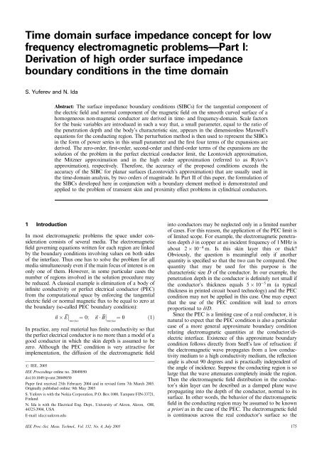
system ða 1 ; a 2 ; ZÞ, related to the body surface (Fig. 1): 

 

@ ðe ak H ak Þ @ e Z H Z 

¼ ð 1Þ 3 k e ak e Z sE x3 

@Z @a 

k 

; k ¼ 1; 2; 

k 

X 2 

i¼1 

ð 

@ ðe ak E ak Þ 

@Z 

X 2 

i¼1 

1Þ @ ðe ai H ai Þ 

@a a3 i 

¼ e a1 e a2 sE Z 

ð9Þ 

 

@ e Z E Z 

¼ ð 1Þ k @H x3 

e ak e Z m k 

@a 1 ; k ¼ 1; 2; 

k @t 

ð 1Þ 3 i @ ðe ai E ai Þ @H Z 

¼ e a1 e a2 m 

@a 1 

a3 i 

@t 

X 2 

i¼1 

 

@ e ai e Z H ai 

þ @ e 

a 1 

e a2 H Z 

¼ 0 

@a a3 i 

@Z 

ξ 1 η 

α 2 

ξ 2 

ð10Þ 

ð11Þ 

Consider a homogeneous body of finite conductivity 

ðE 1 ; m 1 ; s 1 Þ, surrounded by a non-conductive medium 

ðE 2 ; m 2 ; s 2 ¼ 0Þ. The parameters of the conducting material 

are assumed to be constant. Let the characteristic dimension 

of the problem be small compared with the wavelength of 

the incident electromagnetic field. Thus the electric field ~E 

and magnetic field ~H inside the body can be described by 

Maxwell’s equations neglecting the displacement current 

density: 

r~E ¼ 

m 1 

@~H 

@t 

r~H ¼ s~E 

ð4Þ 

ð5Þ 

r~H ¼ 0 

ð6Þ 

The exact boundary conditions at the surface of the 

conductor are 

~n ~H cond 

¼ ~n ~H diel 

; m 1 ~n ~H cond 

¼ m 2 ~n ~H diel 

; 

~n ~E cond 

¼ ~n ~E diel 

; ~n ~E cond 

¼ ~n ~E ð7Þ 

diel 

Let the time variation of the incident field be such that the 

electromagnetic penetration depth d into the body remains 

α 1 

d 2 

d 1 

Fig. 1 Local orthogonal curvilinear co-ordinate systems related to 

the surface 

where e a1 ; e a2 ; e Z are the Lame coefficients. The co-ordinates 

a 1 and a 2 are defined as angles whereas the co-ordinate Z is 

defined as the distance measured from the surface to a 

current point inside the body. The Lame coefficients of the 

co-ordinates ða 1 ; a 2 ; ZÞ arewrittenintheform: 

e a1 ¼ d 1 Z; e a2 ¼ d 2 Z; e Z ¼ 1 ð12Þ 

where d k ; k ¼ 1; 2, are the local radii of curvature of the 

corresponding co-ordinate line. 

In analysis of the skin effect problem using the perturbation 

technique, it is natural to perform derivations in the 

system where all co-ordinates are of the same dimensionality. 

For this purpose we replace the co-ordinates a 1 and a 2 

(angles) by x 1 and x 2 (distances) (Fig. 1). The characteristic 

lengths associated with the co-ordinates x i and Z are D and 


d, respectively. The two co-ordinate systems are related as 

follows: 

x 1 ¼ d 1 a 1 ; x 2 ¼ d 2 a 2 ð13Þ 

Equations (9)–(11) with the co-ordinates in (13) are written 

in the form 

@H xk 

X 2 

@Z 

i¼1 

@E xk 

@Z 

X 2 

i¼1 

d k 

d k 

@H Z 

Z @x k 

@H xi 

H xk 

d k Z ¼ð 1Þ3 k sE x3 k 

; k ¼ 1; 2; 

ð 1Þ i d 3 i 

¼ sE Z 

d 3 i Z @x 3 i 

ð14Þ 

d k 

d k 

@E Z 

Z @x k 

E xk 

d k Z ¼ð @H 1Þk x3 

m k 

1 ; k ¼ 1; 2; 

@t 

@E xi 

ð 1Þ 3 i d 3 i 

d 3 i Z @x 3 

@H Z 

@Z þ X2 

d 

i¼1 i 

d i 

@H Z 

¼ m 1 

i @t 

@H xi 

X 2 

¼ H Z 

Z @x i i¼1 

4 Dimensionless variables 

d i 

ð15Þ 

ð ZÞ 1 ð16Þ 

Following perturbation theory methods, we introduce the 

characteristic scale factors for the variables of the problem. 

The choice of the scale factors for co-ordinates x 1 ; x 2 ; Z is 

evident, namely the characteristic size D ¼ minðd 1 ; d 2 Þ of 

the conductor’s surface for x 1 and x 2 , and the penetration 

depth d for Z. The quantity t was introduced in (8) as the 

ratio 2/o in the case of time-harmonic fields or the incident 

pulse duration in the case of transient sources and is 

therefore the natural scale factor for time. We denote for 

now the scale factors for the electric and magnetic fields as 

E and H , respectively. 

Let us now switch to the following non-dimensional 

variables: 

~x k ¼ x k =D; ~t ¼ t=t; ~Z ¼ Z=d; ~E ¼ E=E ; ~H 

¼ H=H 

ð17Þ 

Here and below, the sign ‘B’ denotes non-dimensional 

quantities. 

Substitution of (17) into (14)–(16) gives 

H 

d 

 

@ ~H xk 

@~Z 

d 

D 

d k 

d k 

@ ~H Z 

d~Z @ ~ x k 

¼ ð 1Þ 3 k E s~E x3 k 

; k ¼ 1; 2 

d k 

~H xk 

d~Z 

 

ð18aÞ 

H X 2 

ð 1Þ i d 3 i @ ~H xi 

D d 

i¼1 3 i d~Z @ ~ ¼ sE ~E Z ð18bÞ 

x 3 i 

E 

 

D @~E xk d k @~E Z 

~E xk 

D d @~Z d k d~Z @ ~ x k 

d k d~Z 

ð19aÞ 

¼ ð 1 

Þ k H @ ~H x3 

m 1 

t @~t 

k 

; k ¼ 1; 2 

E X 2 

ð 1Þ 3 i d 3 i @~E xi H @ ~H Z 

D 

d 

i¼1 

3 i d~Z @ ~ ¼ m 1 

x 3 i 

t @~t 

D @ ~H Z 

d @~Z þ X2 

i¼1 

d i 

d i 

@ ~H xi 

X 

d~Z @ ~ ¼ D ~H 2 

Z 

x i i¼1 

d i 

ð19bÞ 

ð d~Z Þ 1 ð20Þ 

Note that not all scale factors in (18)–(20) are actually 

independent. Indeed, from (8) it follows that 

p 

d ¼ 

ffiffiffiffiffiffiffiffiffiffiffiffiffiffiffiffi qffiffiffiffiffiffiffiffiffiffiffiffiffiffiffiffiffiffiffiffiffi 

t=ðsm 1 Þ ¼ t=ðsm 1 D 2 ÞD ¼ pD; 

qffiffiffiffiffiffiffiffiffiffiffiffiffiffiffiffiffiffiffiffiffi 

ð21Þ 

p ¼ d=D ¼ t=ðsm 1 D 2 Þ 1 

where the parameter p is proportional to the ratio of the 

penetration depth and characteristic size of the conductor’s 

surface. The relation between E and H follows from (19): 

E ¼ m 1D 

t H ð22Þ 

Therefore, the total number of basic scale factors is 3, for 

example: t, D and H . The practical selection of the scale 

factors should be based on the input data of a given 

problem [21]. Sometimes the total current is used as input 

data. In such cases it is natural to use the characteristic 

current I as one of the basic scale factors instead of E or 

H . The relation between I and H can be obtained using 

the Biot-Savart law 

Z 

~H ¼ ð4pÞ 1 ~I ~R=R 3 dl ð23Þ 

L 

Transfer to the non-dimensional variables in (23) gives: 

Z 

~~HH ¼ I ð4pDÞ 1 ~~I ~ 

~R=~R 3 d ~ l ð24Þ 

L 

Thus 

H ¼ I = ð4pD Þ ð25Þ 

Substitution of (21)–(22) into (18)–(19) gives 

p @ ~H xk 

@~Z 

p 2 X2 

i¼1 

@~E xk 

@~Z 

p 2 X2 

i¼1 

p 2 ~H xk 

~d k p~Z 

p 2 dk ~ @ ~H Z 

~d k p~Z @ ~ ¼ð 1Þ 3 k ~E x3 k 

; k ¼ 1; 2; 

x k 

~ 

ð 1Þ i d3 i @ ~H xi 

~d 3 i ~Z @ ~ ¼ ~E Z 

x 3 i 

ð26Þ 

p~E xk 

~d k p~Z 

p d ~ k @~E Z 

~d k p~Z @ ~ ¼ð 1Þ k p @ ~H x3 

x k 

@~t 

~ 

ð 1Þ 3 i d3 i @~E xi 

~d 3 i ~Z @ ~ ¼ @ ~H Z 

x 3 i 

@t 

@ ~H Z 

@~Z 

p ~H Z 

X 2 

i¼1 

1 

~d i p~Z ¼ p X2 

i¼1 

~d i @ ~H xi 

~d i p~Z @ ~ x i 

k 

; k ¼ 1; 2; 

ð27Þ 

ð28Þ 

where ~ d k ¼ d k =D; k ¼ 1; 2. Equations (26)–(28) do not 

contain the scale factors for the electric and magnetic fields 

anymore. The remaining scale factors for the co-ordinates 

are included only in the form of the ratio d/D which is the 

small parameter of the problem. 

5 Expansions in the small parameter 

We now apply Laplace’s transform following the rule 

ef ðesÞ ¼ R 1 

0 

ef ðetÞ expð esetÞdet. Here f denotes an arbitrary 

function. In the Laplace-domain, (26)–(28) are written 


in the form: 

p @ ~H xk 

@~Z 

p 2 X2 

i¼1 

@~E xk 

@~Z 

p 2 X2 

i¼1 

@ ~H Z 

@~Z 

p 2 ~H xk 

~d k p~Z 

p 2 dk ~ @ ~H Z 

~d k p~Z @ ~ ¼ð 1Þ 3 k ~E x3 k 

; k ¼ 1; 2; 

x k 

~ 

ð 1Þ i d3 i @ ~H xi 

~d 3 i ~Z @ ~ ¼ ~E Z 

x 3 i 

ð29Þ 

p~E xk 

~d k p~Z 

p d ~ k @~E Z 

~d k p~Z @ ~ ¼ð 1Þ k p~s ~H x3 k 

; k ¼ 1; 2; 

x k 

~ 

ð 1Þ 3 i d3 i @~E xi 

~d 3 i ~Z @ ~ ¼ ~s ~H Z 

x 3 i 

ð30Þ 

p ~H Z 

X 2 

i¼1 

1 

~d i p~Z ¼ p X2 

i¼1 

~d i @ ~H xi 

~d i p~Z @ ~ x i 

ð31Þ 

Since the parameter p is small, we represent the functions, 

for which the solutions are sought, in the form of 

asymptotic expansions in the parameter p: 

~ 

H ¼ X1 

p m ~ 

H ~ 

m ; E ¼ X1 

p m ~ 

E m ð32Þ 

m¼0 

m¼0 

The following functions can also be represented as 

expansions in the small parameter p: 

1 

~d k p~Z ¼ 1 þ p ~Z þ p 

dk ~ d ~ 2 ~Z2 þ Oðp 

2 

k 

~d 3 Þ 

k 

3 

~d k 

~d k p~Z ¼ 1 þ p ~Z þ p 

dk ~ 2 ~Z2 þ Oðp 

~d 3 Þ 

k 

2 

ð33Þ 

Substituting the expansions (32) and (33) into (29)–(31) 

and equating the coefficients of equal powers of p, the 

following equations for the expansion coefficients are 

obtained: 

m ¼ 0: 

m ¼ 1: 

m ¼ 2: 

@ð ~ ~E 2 Þ xk 

@~Z 

ð ~ ~E 0 Þ x1 

¼ð ~ ~E 0 Þ x2 

¼ð ~ ~E 0 Þ Z 

¼ð ~ ~H 0 Þ Z 

¼ 0 ð34Þ 

@ð ~ ~E 1 Þ xk 

@~Z 

¼ð 1Þ k ~sð ~ ~H 0 Þ x3 k 

k ¼ 1; 2 ð35aÞ 

ð ~ ~E 1 Þ xk 

¼ð 1Þ k @ð~ ~H 0 Þ x3 k 

@~Z 

X 2 

i¼1 

k ¼ 1; 2 

ð35bÞ 

ð 1Þ i @ð ~E ~ 1 Þ x3 k 

@ ~ ¼ ~sð ~ ~H 1 Þ Z 

ð35cÞ 

x i 

@ð ~ ~H 1 Þ Z 

@Z 

¼ 

X2 

i¼1 

ð ~ ~E 1 Þ Z 

¼ 0 

@ð ~ ~H 0 Þ xi 

@x i 

ð35dÞ 

ð35eÞ 

¼ ð~ ~E 1 Þ xk 

~d k 

þð 1Þ k ~sð ~ ~H 1 Þ x3 k 

k ¼ 1; 2 ð36aÞ 

2 

ð ~ ~E 2 Þ xk 

¼ð 1Þ k @ð ~ ~H 1 Þ 

4 x3 k 

@~Z 

X 2 

i¼1 

@ð ~ ~H 2 Þ Z 

@~Z 

m ¼ 3: 

@ð ~ ~E 3 Þ xk 

@~Z 

ð ~ ~E 3 Þ xk 

2 

ð ~ ~H 0 Þ x3 

~d 3 k 

k 

3 

5 k ¼ 1; 2 ð36bÞ 

ð 1Þ i @ð ~ ~E 2 Þ x3 i 

@ ~ þ ~Z @ð ~ ~E 1 Þ 

4 

x3 i 

x i di ~ @ ~ 5 ¼ ~sð ~ ~H 2 Þ Z 

ð36cÞ 

x i 

ð ~ ~E 2 Þ Z 

¼ X2 

¼ð ~ ~H 1 Þ Z 

X 2 

i¼1 

i¼1 

~d 1 

i 

3 

ð 1Þ 3 i @ð ~H 0 Þ x3 i 

@x i 

X 2 

i¼1 

2 

@ð ~ ~H 1 Þ 

4 xi 

@ ~ x i 

þ ~Z ~ di 

@ð ~ ~H 0 Þ xi 

@ ~ x i 

ð36dÞ 

3 

5 

ð36eÞ 

¼ ð~ ~E 2 Þ xk 

þ ~Z ð~ ~E 1 Þ xk 

þ @ð~ ~E 2 Þ Z 

~d k 

~d 

k 

2 @ ~ þð 1Þ k ~sð ~ ~H 2 Þ x3 

x 

k 

k 

2 

k ¼ 1; 2 

¼ð 1Þ k @ð ~ ~H 2 Þ 

4 x3 k 

@~Z 

X 2 

i¼1 

k ¼ 1; 2 

ð ~ ~H 1 Þ x3 k 

~Z ð~ ~H 0 Þ x3 k 

~d 3 k 

~d 2 3 k 

2 

ð 1Þ i @ð ~ ~E 3 Þ x3 i 

@ ~ þ ~Z @ð ~ ~E 2 Þ x3 i 

x i di ~ @ ~ þ ~Z2 @ð ~ 3 

~E 1 Þ 

4 

x3 i 

x i @ ~ 5 

x i 

¼ ~sð ~ ~H 3 Þ Z 

ð ~ ~E 3 Þ Z 

¼ X2 

i¼1 

2 

@ð ~ ~H 3 Þ Z 

¼ð ~ X 

~H 2 

2 Þ 

@~Z 

Z 

2 

X 2 @ð ~ ~H 2 Þ 

4 xi 

@ ~ x i 

i¼1 

~d 2 i 

ð37aÞ 

3 

@ð ~ ~H 1 Þ Z 

@ ~ 5 

x 3 k 

ð37bÞ 

ð37cÞ 

ð 1Þ 3 i @ð ~ ~H 1 Þ x3 i 

@ ~ þ ~Z @ð ~ ~H 0 Þ 

4 

x3 i 

x i di ~ @ ~ 5 ð37dÞ 

x i 

i¼1 

~d 1 

i þ ~Zð ~ ~H 1 Þ Z 

X 2 

þ ~Z ~ di 

@ð ~ ~H 1 Þ xi 

@ ~ x i 

þ ~Z2 

~d 2 i 

i¼1 

~d 2 

i 

3 

@ð ~ ~H 0 Þ xi 

@ ~ 5 

x i 

3 

ð37eÞ 

The procedure described above can be continued and the 

equations for the following terms of expansions can be 

derived. However, in the present paper we restrict ourselves 

to four terms of the expansions (m ¼ 3) and neglect the 

terms of the order O(p 4 ). Note that the use of higher order 

SIBCs for practical computations is restricted, because one 

has to compute (or aprioriknow) the principal curvatures 

at every point. 

The representation (32) has clear physical meaning, 

namely: 

(1) The zero-order terms of the expansions (32) give the 

solution of the problem in so-called perfect electrical 

conductor limit (PEC), in which the magnetic field diffusion 

into the body is neglected. 


(2) The first-order terms describe the diffusion in the wellknown 

Leontovich approximation, in which the body’s 

surface is considered as a plane and the field is assumed to 

penetrate into the body only in the direction normal to the 

body’s surface. 

(3) The second-order terms provide a correction that takes 

into account the curvature of the body’s surface, but the 

diffusion is assumed to be only in the direction normal to 

the surface as in the Leontovich approximation. This is 

Mitzner’s approximation. 

(4) The third-order terms and higher allow for the magnetic 

field diffusion in directions tangential to the body’s surface. 

This approximation will be referred as Rytov’s approximation. 

Below, the problems described by (35)–(37) are solved 

sequentially to derive the first-, second- and third-order 

terms in explicit form. 

6 Surface impedance boundary conditions in the 

Laplace domain 

6.1 Leontovich’s approximation 

The first-order terms of the expansions of the electric and 

magnetic fields at the body’s surface (Z ¼ 0) can be 

expressed directly from (35b) and (35c) as follows: 

ð~E 1 Þ b x k 

¼ð 1Þ k @ð~ ~H 0 Þ x3 k 

@~Z 

k ¼ 1; 2 ð38aÞ 

 

~Z¼0 

X 2 

ð ~ ~H 1 Þ b Z ¼ 1 ð 1Þ i @ð~ ~E 1 Þ b x 3 i 

~s 

i¼1 @ ~ ð38bÞ 

x i 

Here and below, the superscript ‘b’ denotes quantities on 

the surface of the conductor. The distribution of the 

functions ð ~ ~H 0 Þ xi 

in the direction normal to the body’s 

surface is described by the following 1-dimensional diffusion 

equation obtained from (35a) and (35b): 

@ 2 ð ~ ~H 0 Þ xk 

@~Z 2 ~sð ~ ~H 0 Þ xk 

¼ 0 k ¼ 1; 2 ð39Þ 

Equation (39) must be supplemented by the following 

conditions: 

~Z ¼ 0 : ð ~ ~H 0 Þ xk 

¼ð ~ ~H 0 Þ b x k 

; Z !1: ð ~ ~H 0 Þ xk 

! 0 ð40Þ 

Thesolutionof(39)and(40)iswrittenintheform: 

ð ~ ~H 0 Þ xk 

¼ð ~ p 

~H 0 Þ b x k 

exp ~Z ~s 

ffiffi 

; k ¼ 1; 2 ð41Þ 

By substituting (41) into (38a) and (38b), the functions 

ð ~ ~E 1 Þ b x k 

and ð 

~~H ~ 1 Þ b Z 

are obtained: 

ð ~ pffiffi 

~E 1 Þ b x k 

¼ð 1Þ 3 k ~ 

~s ð H 0 Þ b x 3 k 

; k ¼ 1; 2 ð42aÞ 

ð ~ ~H 1 Þ b Z ¼ p 1 ffiffi 

X2 @ð ~ ~H 0 Þ b x i 

~s 

i¼1 @ ~ ð42bÞ 

x i 

Since the zero-order terms of the expansions of the 

functions ~E b xi and ~H b Z are zero, the Leontovich order SIBC 

in the Laplace domain can be written from (42a) and (42b) 

as follows: 

~E b pffiffi 

x k 

¼pð 1Þ 3 k ~ 

~s ð H 0 Þ b x 3 k 

þ Oðp 2 Þ 

p ffiffi 

¼pð 1Þ 3 k ~s H ~ b x 3 k 

þ Oðp 2 Þ k ¼ 1; 2 

~H b Z ¼ p ffiffi 

X2 @ð ~ ~H 0 Þ b x i 

~s 

i¼1 @ ~ þ Oðp 2 Þ 

x i 

ð43aÞ 

¼ p ffiffi 

X2 @ð ~HÞ b x i 

~s 

i¼1 @ ~ þOðp 2 Þ ð43bÞ 

x i 

Note that (42a) and (42b) can also be obtained by 

integrating (35a) and (35d) over the boundary layer with 

respect to Z: 

ð ~ 

~Z¼1 

~E 1 Þ xk 

¼ ð ~ Z 1 

~E 1 Þ b x k 

¼ð 1Þ k ~s ð ~ ~H 0 Þ x3 k 

d~Z 

~Z¼0 

0 

ð44aÞ 

k ¼ 1; 2 

ð ~ 

~Z¼1 

~H 1 Þ Z 

¼ ð ~ ~H 1 Þ b Z ¼ X2 

~Z¼0 

i¼1 

Z 

@ 1 

@ ~ ð ~ ~H 0 Þ xi 

d~Z 

x i 

0 

ð44bÞ 

It is a simple matter to verify that substitution of (41) into 

(44a) and (44b) leads to (43a) and (43b). 

6.2 Mitzner’s approximation 

The functions ð ~ ~E 2 Þ b x k 

and ð ~ ~H 2 Þ b Z 

can be derived from (36b) 

and (36c) as follows: 

2 

ð ~ ~E 2 Þ b x k 

¼ð 1Þ k @ð ~ ~H 1 Þ x3 k 

ð ~ 3 

6 

~H 0 Þ b x 3 k 7 

4 

@~Z 

5 

~d 3 k ð45aÞ 

~Z¼0 

k ¼ 1; 2 

ð ~ ~H 2 Þ b Z ¼ 1 s 

X 2 

i¼1 

ð 1Þ i @ð~ ~E 2 Þ b x 3 

@ ~ x i 

i 

ð45bÞ 

The diffusion equation for the functions ð ~ ~H 1 Þ x1 

can be 

obtained from (36a) and (36b) and written in the following 

form: 

@ 2 ð ~ ~H 1 Þ x3 k 

@~Z 2 ~sð ~ ~H 1 Þ x3 k 

¼ d ~ 1 @ð ~ ~H 0 Þ x3 

3 k 

@~Z 

þð 1Þ k ~ d 

1 

k ð ~ ~E 1 Þ xk 

; k ¼ 1; 2 

k 

ð46Þ 

Note that the right-hand side of (46) is not zero unlike the 

diffusion equation (39) for ð ~ ~H 0 Þ x1 

in the Leontovich 

approximation. Taking into account (41) and (35b), one 

obtains: 

ð 1Þ k ð ~ ~E 1 Þ xk 

¼ @ð~ ~H 0 Þ x3 k 

@~Z 

k ¼ 1; 2 

¼ 

Substitution of (47) into (46) yields: 

pffiffi 

~ p 

~s ð H 0 Þ b x 3 k 

expð ~Z ~s 

ffiffi Þ 

ð47Þ 

@ 2 ð ~ ~H 1 Þ x3 k 

~sð ~ ~H 

@~Z 2 1 Þ x3 k 

ð48Þ 

¼ d ~ pffiffi 

~ p 

12 ~s ð H 0 Þ b x 3 k 

expð ~Z ~s 

ffiffi Þ k ¼ 1; 2 


where d ~ 12 ¼ P2 ~d i 

1 . Equation (48) must be supplemented 

i¼1 

by the following conditions: 

~Z ¼ 0 : ð ~ ~H 1 Þ xk 

¼ð ~ ~H 1 Þ b x k 

ð ~ x 1 ; ~ x 2 ;~sÞ; 

~Z !1: ð ~ ~H 1 Þ xk 

! 0 k ¼ 1; 2 

Thesolutionof(48)and(49)iswrittenintheform 

ð49Þ 

By combining (43) and (51) the Mitzner order SIBCs in 

the Laplace domain are written in the following form: 

~E b p 

x k 

¼ð 1Þ 3 k p ~s 

ffiffi 

ð 

~~H 0 Þ b x 3 k 

þp ð ~ ~H 1 Þ b x 3 k 

þ 1 

 

p 

2 ~s 

ffiffi d ~ 1 

3 k 

~d k 

1 

ð 

~~H 0 Þ b x 3 k 

þ Oðp 3 Þ 

ð53aÞ 

p 

¼ð 1Þ 3 k p ~s 

ffiffi 1 þ p 

2 ~s 

ffiffi d ~ 1 

3 k 

~d k 

1 ~ ~H b x 3 k 

þ Oðp 3 Þ k ¼ 1; 2 

ð ~ 

~H 1 Þ x3 k 

¼ ð ~ ~H 1 Þ b x 3 k 

þ ~Z d 

2 ~ 12 ð ~ 

~H 0 Þ b p 

x 3 k 

expð ~Z 

ffiffi s Þ 

k ¼ 1; 2 

ð50Þ 

By substituting (50) into (45), the functions ð ~ ~E 2 Þ b ð ~ ~H 2 Þ b Z are 

finally obtained: 

~H b Z ¼ 

pffiffi 

X2 @ b 

~H 

~s 

i¼1 @ ~ 0 

x i 

x k 

b 

þ p 

~H 1 þ p 1 

x i 2 ~s 

ffiffi d ~ 1 

i 

¼ p ffiffi 

X2 

~s 

i¼1 

 

 

1 þ p 

ffiffi 

~s 

~d 1 

i 

 

~d 3 i 1 ~H 0 

b 

x i 

 

þ Oðp 3 Þ 

~d 3 1 @ ~H b x i 

i 

@ ~ þ Oðp 3 Þ 

x i 

ð53bÞ 

ð ~ 

ffiffi 

~E 2 Þ b x k 

¼ð 1Þ 3 k ~s 

k ¼ 1; 2 

p ~ ð H 1 Þ b x 3 k 

þ 1 

d 

2 ~ 1 

~ 

x 3 k 

d 

1 

k 

 

ð ~ ~H 0 Þ b x 3 

k 

 

ð51aÞ 

6.3 Rytov’s approximation 

From (37b) and (37c) one obtains: 

2 

ð ~E ~ 3 Þ b x k 

¼ð 1Þ k @ð ~ ~H 2 Þ x3 k 

ð ~ ~H 1 Þ b x 3 k 

@ð ~ 3 

6 

~H 1 Þ b Z7 

4 

@~Z 

~d 3 k @ ~ 5 

x 3 k 

~Z¼0 


X2 @ð ~ ~H 1 Þ b x i 

~s 

i¼1 @ ~ x i 

k ¼ 1; 2 

ð54aÞ 

þ 1 2~s 

X 2 

i¼1 

~d 1 

i 

~d 3 1 @ð ~ ~H 0 Þ b x i 

i 

@ ~ x i 

ð51bÞ 

ð ~ ~H 3 Þ b Z ¼ 1 ~s 

X 2 

i¼1 

ð 1Þ i @ð~ ~E 3 Þ b x 3 

@ ~ x i 

i 

ð54bÞ 

Another way to obtain the formulae in (51) is by 

integration of (36a) and (36e) over the boundary layer as 

follows: 

The distribution of the functions ð ~ ~H 2 Þ xi 

over the boundary 

layer is described by the following 1-dimensional problem 

obtained from (37a) and (37b): 

ð ~ ~H 1 Þ b Z ¼ 

ð ~ ~E 2 Þ b x k 

¼ ~ d 1 

k 

k ¼ 1; 2 

X2 

i¼1 

þ X2 

i¼1 

~d 1 

i 

Z 1 

0 

þð 1Þ 3 

Z 1 

0 

Z 

@ 1 

@ ~ x i 0 

ð ~ ~E 1 Þ xk 

d~Z 

Z 1 

k s 

0 

ð ~ ~H 1 Þ Z 

d~Z 

 

ð ~ ~H 1 Þ xi 

þ ~ d 1 

i 

ð ~ ~H 1 Þ x3 k 

d~Z 

Substitution of (52) into (45) leads to (51). 

~Zð ~ ~H 0 Þ xi 

 

d~Z 

ð52aÞ 

ð52bÞ 

@ 2 ð ~ ~H 2 Þ x3 k 

~sð ~ ~H 

@~Z 2 2 Þ x3 k 

¼ ð 1Þk ð ~ ~E 2 Þ xk 

þ ð 1Þk ~Zð ~ ~E 1 Þ xk 

~d k 

þð 1Þ k @ð~ ~E 2 Þ Z 

@ ~ þ 1 @ð ~ ~H 1 Þ x3 k 

x k 

~d 3 k @~Z 

þ ~Z 

~d 2 3 k 

@ð ~ ~H 0 Þ x3 

@~Z 

k 

þ @2 ð ~ ~H 1 Þ Z 

@ ~ x 3 k @~Z 

~Z ¼ 0 : ð ~ ~H 2 Þ xk 

¼ð ~ ~H 2 Þ b x k 

ð ~ x 1 ; ~ x 2 ;~sÞ; 

~Z !1: ð ~ ~H 2 Þ xk 

! 0 

~d 2 k 

þ ð~ ~H 0 Þ x3 

k ¼ 1; 2 

~d 2 3 k 

k 

ð55aÞ 

ð55bÞ 

Substituting the solution of the problem in (55) into (54) 

and combining the result with (53), the Rytov order SIBC in 

the Laplace domain is written in the following form (details 


of this derivation are given in the Appendix): 

~E b pffiffi 

x k 

¼ð 1Þ 3 k ~s 

( 

p þ p2 d 

p ffiffi 

~ k d3 ~ k 

~s 2 d ~ þ p3 3 d ~ k 

2 ~d 3 2 k 2 ~ ! 

d k d3 ~ k 

k d3 ~ k 

~s 8 d ~ k 2 d ~ ~H b 

3 2 x 3 k 

: 

k 

0 

þ p3 @ 2 ~H b x 3 k 

þ @2 ~H b x 3 k 

þ 2 

@2 ~H b 1) 

@ 

x k A 

2~s 

@x 3 k @x k 

@x 2 k 

þ Oðp 4 Þ k ¼ 1; 2 

~H b Z ¼ p 2 ffiffi 

X2 

~s 

i¼1 

( 

@ 

@ ~ x i 

þ p2 3 d ~ 3 2 i 

~s 

þ p2 

2~s 

þ Oðp 4 Þ 

@x 2 3 

k 

p þ p2 d 

p ffiffi 

~ 3 i di ~ 

~s 2 d ~ i d3 ~ i 

! 

~H b x i 

~d 2 i 2 ~ d i 

~ d3 i 

8 ~ d 2 i ~ d 2 3 i 

@ 2 ~H b x i 

@ ~ x 2 3 i 

þ @2 ~H b x i 

@ x 2 i 

þ 2 @2 ~H b !) 

x 3 i 

@ x i @ x 3 i 

ð56aÞ 

ð56bÞ 

The conditions (56) can also be represented in the following 


~E b x k 

¼ð 1Þ 3 k ~s~F 3 k k ¼ 1; 2 ð57aÞ 

~F 3 k ¼ p~T 1 ~ ~H x b 3 k 

þ p ~ 2 d k d3 ~ k 

2 d ~ ~T 

k d3 ~ 2 ~ ~H x b 3 k 

k 

þ p 3 3~ dk 

2 ~d 3 2 k 2 d ~ k d3 ~ k 

8 d ~ k 2 d ~ ~T 

3 2 3 ~ ~H x b 3 k 

k 

! 

þ p3 

T 

2 ~ @ 2 ~H 

x b 

3 ~ 

3 k 

@ ~ x 2 þ @2 ~H 

x b 3 k 

k @ ~ x 2 þ 2 

@2 ~H 

x b k 

3 k @ ~ x k @ ~ x 3 k 

þ Oðp 4 Þ k ¼ 1; 2 

ð59cÞ 

where the sign ‘~’ denotes a time convolution product with 

respect to non-dimensional time. 

The functions F k describe the perturbation of the external 

field surrounding the body owing to the field diffusion into 

the body and dissipation of the energy by the body. The 

first term on the right-hand side of (59c) gives the 

contribution from the field diffusion in the direction normal 

to the planar surface. The second and third terms give a 

correction due to the curvature. The fourth term takes into 

account the field diffusion in the directions tangential to the 

planar surface. The functions T m describe the evolution of 

these processes in time. 

The SIBC for the tangential electric field can be 

represented in a more traditional form than (59a): 

~H b Z ¼ X2 @ ~F i 

@ ~ x i 

i¼1 

ð57bÞ 

( 

~E b x k 

¼ð 1Þ 3 k p ~^T 1 ~ ~H b x 3 k 

þ p ~ d k 

~ d3 k 

2 ~ d k 

~ d3 k 

~^T 2 ~ ~H b x 3 k 

where the Laplace-domain functions ~F k ¼ ~F k ð ~ x 1 ; ~ x 2 ;~sÞ; k 

¼ 1; 2; are as follows 

~F 3 k ¼ p ffiffi ~H b x 

~s 3 k 

þ p2 ~d k d3 ~ k 

~s 2 d ~ ~H b 

k d3 ~ x 3 k k 

þ p3 3 d ~ k 

2 ~d 3 2 k 2 d ~ k d3 ~ k 

~s 8 d ~ k 2 d ~ ~H b 

3 2 x 3 k 

k 

0 

þ p3 @ 2 ~H b x 3 k 

2~s 3=2 @ ~ x 2 þ @2 ~H b x 3 k 

k @ ~ x 2 þ 2 

@2 ~H b 

@ 

x k 

3 k @ ~ x k @ ~ x 3 

þ Oðp 4 Þ 

k 

1 

A 

ð57cÞ 

7 Surface impedance boundary conditions in the 

time domain 

Using the inverse Laplace transform, the following timedomain 

functions T m are derived [22]: 

1 

p ffiffi , 

1 1 

pffiffiffiffi 

¼ ~T 1 ð~tÞ; 

~s p~t ~s , Uð ~tÞ¼~T 2 ð~tÞ; 

1 

~s , 2 p 

pffiffiffi 

~t 

ffiffi ¼ ~T 3=2 3 ð~tÞ 

p 

ð58Þ 

where U(t) is the unit step function. Substituting (58) into 

(57) and applying the Duhamel theorem, one obtains: 

~E b x k 

¼ð 1Þ 3 k @ ~F 3 k 

~@t 

~H b Z ¼ X2 

i¼1 

@ ~F i 

@ ~ x i 

ð59aÞ 

ð59bÞ 

where 

þp 2 3~ d 2 k 

þ p2 

2 

~^T 3 ~ 

~d 3 2 k 2 d ~ k d3 ~ k ~^T 

8 d ~ k 2 d ~ 3 2 3 ~ ~H x b 3 

k 

@ 2 ~H b x 3 

@ ~ x 2 k 

þ Oðp 4 Þ k ¼ 1; 2 

~^T 1 ð~tÞ ¼ ð4pÞ 1=2 ~t 3=2 ; 

~^T 3 ð~tÞ¼p 1=2 ~t 1=2 

where U 0 ð~tÞ is the delta-function. 

k 

þ @2 ~H 

x b 3 

@ ~ x 2 3 

k 

k 

k 

!) 

þ 2 

@2 ~H 

x b k 

@ ~ x k @ ~ x 3 k 

~^T 2 ð~tÞ¼U 0 ð~tÞ; 

Table 1: Quantities and appropriate scale factors 

Quantity Scale factor Unit 

@=@x 1 , @=@x 2 D 1 m 1 

E 

H 

ð4pÞ 1 I t 1 Vm 1 

ð4pÞ 1 I D 1 Am 1 

T k , k ¼ 1,2,3 ðsm 0 Þ k=2 ðk 1Þ=2 

t m k s 1 

¼ p k t 1 D k 

dt (in time convolution product) t s 

ð59dÞ 

ð60Þ 


Returning to dimensional variables in (59) gives (see 

Table 1): 

( 

Ex b k 

¼ð 1Þ 3 k ^T 1 Hx b 3 k 

þ d k d 3 k 

^T 2 Hx b 2d k d 3 k 

: 

3 k 

þ 3d2 k d3 2 k 2d k d 3 k 

8dk 2d2 3 k 

þ ^T 3 

2 @ 2 Hx b 3 k 

@x 2 þ @2 Hx b 3 

k @x 2 3 

k ¼ 1; 2 

H b Z ¼ X2 

i 1 

^T 3 H b x 3 

k 

k 

k 

!) 

þ 2 

@2 Hx b k 

þ ... 

@x k @x 3 k 

( 

@ 

T 1 Hx b @x i 

þ d 3 i d i 

T 2 Hx b 

i 2d i d i 

: 

3 i 

þ 3d2 3 i di 2 2d i d 3 i 

8di 2 T 3 H d2 x b i 

3 i 

þ T 3 

2 @ 2 Hx b i 

@x 2 þ @2 Hx b i 

3 i @x 2 i 

þ ... 

!) 

þ 2 @2 Hx b 3 i 

@x i @x 3 i 

ð61aÞ 

ð61bÞ 

where T 1 ðtÞ¼ðpsmÞ 1=2 t 1=2 ; T 2 ðtÞ¼UðtÞ=ðsmÞ; 

T 3 ðtÞ ¼2 ps 3 m 3 1=2 

t 1=2 ; ^T 1 ðtÞ¼ ð4ps=mÞ 1=2 t 3=2 ; 

^T 2 ðtÞ ¼U’ðtÞ=s; and^T 3 ðtÞ¼ ps 3 m 1=2 

t 1=2 . 

The time domain surface impedance boundary conditions 

in (61) are the first main result of this work. 

As a conclusion of this Section let us demonstrate how 

the original frequency domain Mitzner’s and Rytov’s 

conditions can be obtained from (56). Since the ratio 2/o 

is the time scale factor in the time harmonic case, all we 

have to do is to replace ~s by 2j as follows: 

( 

~_E b x k 

¼ð 1Þ 3 k pð1 þ jÞ 1 þ p 1 j 

 

: 

þ p2 3 d ~ k 

2 

2j 

þ p3 

2j 

~d 2 3 k 2 ~ d k 

~ d3 k 

8 ~ d 2 k ~ d 2 3 k 

@ 2 ~ _H b x 3 

@ ~ x 2 k 

þ Oðp 4 Þ k ¼ 1; 2 

k 

~ þ @2 _H b x 3 

@ ~ x 2 3 

k 

4 

# 

~_H b x 3 k 

k 

~d 1 

3 k 

~d 1 

k 

~ 

þ 2 

@2 _H b !) 

x k 

@ ~ x k @ ~ x 3 k 

ð62Þ 

where the sign ‘’ denotes the amplitude of the function. 

Substitution of the scale factors gives the condition in 

dimensional form 

( 

_E x b k 

¼ð 1Þ 3 k ð1 þ jÞZ o 

þ d2 

2j 

þ d2 

4j 

3dk 2 d3 2 k 2d k d 3 k 

8dk 2d2 3 k 

@ 2 _H 

x b 3 k 

@x 2 k 

þ ... k ¼ 1; 2 

 

1 þ 1 j 

4 d d 3 1 

k dk 

1 

: 

 

_H x b 3 k 

!) 

þ @2 _H 

x b 3 k 

þ 2 

@2 _H 

x b k 

@x k @x 3 k 

@x 2 3 

k 

ð63Þ 

It is easy to see that by neglecting the terms of the order 

Oðp 3 Þ, the formula (63) reduces to the Mitzner condition 

[8]. Alternatively, by setting d 1 !1, d 2 !1 in (63) the 

Rytov condition [7] is obtained. 

8 Conclusions 

The problem of the diffusion of the transient electromagnetic 

field in a conductor has been solved using the method 

of perturbations in the small parameter p that is equal to the 

ratio of the electromagnetic penetration depth and characteristic 

dimension of the body. The time domain solutions 

for the tangential component of the electric field and the 

normal component of the magnetic field on the smooth 

curved surface of the body (the surface impedance 

boundary conditions) have been obtained with accuracy 

up to Oðp 4 Þ. It was shown that the proposed SIBC in the 

frequency domain generalises the well-known Leontovich 

boundary condition and Mitzner’s boundary condition, 

which provide approximation accuracy within the errors 

Oðp 2 Þ and Oðp 3 Þ, respectively. In Part II of this paper, we 

demonstrate the formulation of the SIBCs developed here 

in conjunction with a boundary element method and apply 

it to the problem of transient skin and proximity effect 

problems in cylindrical conductors. 

9 References 

1 Leontovich, M.A.: ‘On the approximate boundary conditions for the 

electromagnetic field on the surface of well conducting bodies’, in 

Vvedensky, B.A. (Ed.): ‘Investigations of radio waves’ (Acad. of 

Sciences of USSR, Moscow, 1948), pp. 5–12 (in Russian) 

2 Shelkunoff, S.A.: ‘The impedance concept and its application to 

problems of reflection, radiation, shielding and power absorption’, 

Bell Syst. Tech. J., 1938, 17, pp. 17–48 

3 Shchukin, A.N.: ‘Propagation of radio waves’ (Moscow Svyazizdat, 

1940), pp. 48–56 (in Russian) 

4 Smith, G.S.: ‘On the skin effect approximation’, Am. J. Phys., 1990, 

58, (10), pp. 996–1002 

5 Godzinski, Z.: ‘The surface impedance concept and the theory of 

radio waves over real earth’, Proc. IEE, 1961, 108C, pp. 362–373 

6 Wait, J.R.: ‘The ancient and modern history of EM ground-wave 

propagation’, IEEE Antennas Propag. Mag., 1998, 40, (5), pp. 7–24 

7 Ishimaru, A., Rockway, J.D., Kuga, Y., and Lee, S.W.: ‘Sommerfeld 

and Zenneck wave propagation for a finitely conducting onedimensional 

rough surface’, IEEE Trans. Antennas Propag., 2000, 

48, (9), pp. 1475–1484 

8 Rytov, S.M.: ‘Calculation of skin effect by perturbation method’, 

Zhurnal Experimental’noi i Teoreticheskoi Fiziki, 1940, 10, (2), pp. 

180–189 (in Russian) 

9 Mitzner, K.M.: ‘An integral equation approach to scattering from a 

body of finite conductivity’, Radio Sci., 1967, 2, (12), pp. 1459–1470 

10 Hoole, S.R.H., and Carpenter, J.: ‘Surface impedance models for 

corners and slots’, IEEE Trans. Magn., 1985, 21, (5), pp. 1841–1843 

11 Deeley, E.M.: ‘Surface impedance near edges and corners in 3D 

media’, IEEE Trans. Magn., 1990, 26, (2), pp. 712–714 

12 Wang, J., Lavers, J.D., and Zhou, P.: ‘Modified surface impedance 

boundary conditions for 3D eddy current problems’, IEEE Trans. 

Magn., 1993, 29, (2), pp. 1826–1829 

13 Park, Y.G., Chung, T.K., Jung, H.K., and Hahn, S.Y.: ‘Three 

dimesional eddy current computation using the surface impedance 

method considering geometric singularity’, IEEE Trans. Magn., 1995, 

31, (3), pp. 1400–1403 

14 Yuferev, S., Proekt, L., and Ida, N.: ‘Surface impedance boundary 

conditions near corners and edges: rigorous consideration’, IEEE 

Trans. Magn., 2001, 37, (5), pp. 3465–3468 

15 Karp, S.N., and Karal, F.C.: ‘Generalized impedance boundary 

conditions with applications to surface wave structures’, in Brown, J. 

(Ed.): ‘Electromagnetic wave theory, Pt. 1’ (Pergamon, New York, 

1965), pp. 479–483 

16 Senior, T.B.A., and Volakis, J.L.O.: ‘Approximate boundary conditions 

in electromagnetics’, in ‘IEE Electromagn. Wave Ser.’ (IEE, 

London, 1995) 

17 Hoppe, D.J., and Rahmat-Samii, Y.: ‘Impedance boundary conditions 

in electromagnetics’ (Taylor and Francis, Washington, DC, 1994) 

18 Marceaux, O., and Stupfel, B.: ‘High-order impedance boundary 

conditions for multilayer coated 3-D objects’, IEEE Trans. Antennas 

Propag., 2000, 48, (3), pp. 429–436 

19 Yuferev, S., and Yuferev, V.: ‘Diffusion of the electromagnetic field in 

systems of parallel conductors of arbitrary cylindrical shape on 

passage of short current pulses’, Sov. Phys. Tech. Phys., 1991, 36, (11), 

pp. 1208–1212 

20 Yuferev, S., and Kettunen, L.: ‘A unified surface impedance concept 

for both linear and non-linear skin effect problems’, IEEE Trans. 

Magn., 1999, 35, (3), pp. 1454–1457 


21 Yuferev, S., and Ida, N.: ‘Selection of the surface impedance boundary 

conditions for a given problem’, IEEE Trans. Magn., 1999, 35,(3),pp. 

1486–1489 

22 Abramowitz, M. and Stegun, I.A. (Eds.) ‘Handbook of mathematical 

functions with formulas, graphs and mathematical tables’ (National 

Bureau of Standards, 1964) (Applied Math Series *55) 

10 Appendix 

10.1 Calculation of the Rytov order terms of 

expansions of the tangential electric and normal 

magnetic fields at the conductor’s surface 

1. From (36b), (41) and (48) we obtain 

2 

ð 1Þ k ð~ ~E 2 Þ xk 

¼ 1 @ð ~ ~H 1 Þ x3 k 

ð ~ 3 

~H 0 Þ 

4 

x3 k 5 

~d k dk ~ @~Z ~d 3 k 

" 

¼ 1 ð ~ pffiffi 

~H 

dk ~ 1 Þ h d12 ~ 

x 3 k 

~s þ 

2 ð~ ~H 0 Þ b x 3 k 

where d ~ 12 ¼ P2 ~d i 1 . 

i¼1 

2. From (35b) and (41), 

d 

~Z ~ 12 

2 ð~ pffiffi 

~H 0 Þ b ð ~ 3 

~H 0 Þ b 

x 

x 3 k 

~s 

3 k 

p 

5 exp ~Z ffiffi 

~s 

~d 3 k 

ð 1Þ k 

~Zð ~ ~E 

~d 

k 

2 1 Þ xk 

¼ ~Z @ð ~ ~H 0 Þ x3 k 

d ~ 2 

k 

@~Z 

¼ ~Z ð ~ pffiffi 

pffiffi 

~H 

d ~ 2 0 Þ b x 3 k 

~s exp ~Z ~s 

k 

3. From (36d) and (41), 

ð 1Þ k @ð~ ~E 2 Þ Z 

@ ~ x k 

¼ X2 

i¼1 

¼ X2 

i¼1 

4. From (35d) and (41), 

@ 2 ð ~ ~H 1 Þ Z 

@ ~ x 3 k @~Z ¼ X2 

i¼1 

ð 1Þ 3 iþk @2 ð ~ ~H 0 Þ x3 i 

@ ~ x k @ ~ x i 

ð64Þ 

ð65Þ 

ð 1Þ 3 iþk @2 ð ~ ~H 0 Þ 

x3 i 

p 

@ ~ x k @ ~ exp ~Z ~s 

ffiffi 

x i 

@ 2 ð ~ ~H 0 Þ xi 

@ ~ x 3 k 

~ xi 

¼ X2 

i¼1 

ð66Þ 

@ 2 ð ~ ~H 0 Þ b 

x i 

p 

@ ~ exp ~Z ffiffi 

~s 

x 3 k 

~ xi 

ð67Þ 

By using (64)–(67), (55a) can be represented in the following 


@ 2 ð ~ ~H 2 Þ x3 k 

~sð ~ ~H 

@~Z 2 2 Þ x3 k 

¼ð~G 3 k 

p 

þ ~Z ~W 3 k Þ exp ~Z ~s 

ffiffi 

ð68Þ 

where the functions ~G 3 k and ~W 3 k , k ¼ 1, 2, are defined as 

follows 

~G 3 k ¼ d ~ 12 ð ~ pffiffi 

d ~ 

~H 1 Þ s 2 

x 3 k 

~s þ 12 

2 ð~ ~H 0 Þ b x 3 k 

þ ð~ ~H 0 Þ b 

x 3 k 

1 1 

~d 3 k 

~d 3 k 

~d k 

2 

þ X2 

ð 1Þ 3 iþk @2 ð ~ ~H 0 Þ b x 3 i 

@ 2 ð ~ 3 

~H 0 Þ b 

4 

x 

@ ~ x k @ ~ i 

x i @ ~ x 3 k @ ~ 5 

x i 

i¼1 

¼ d ~ 12 ð ~ pffiffi 

~H 1 Þ b 3 d 

x 3 k 

~s 

~ 2 þ 

k þ d ~ 3 

2 

2 d ~ k 2 d ~ 3 2 k 

2 

þ4 

~W 3 k ¼ 

@ 2 ð ~ ~H 0 Þ b x 3 

@ ~ x 2 k 

k 

þ @2 ð ~ ~H 0 Þ b x 3 

@ ~ x 2 3 k 

k 

k 

ð ~ ~H 0 Þ b x 3 

pffiffi 

3 d 

~s 

~ k 2 þ 3~ d3 2 k þ 2~ d k d3 ~ k 

2 d ~ k 2 d ~ 3 2 k 

þ 2 @2 ð ~ ~H 0 Þ b x k 

@ ~ x 3 k @ ~ 5 

x k 

k 

3 

ð69aÞ 

ð ~ ~H 0 Þ b x 3 k 

ð69bÞ 

The solution of equation (68) with the conditions (55b) is 

writtenintheform: 

ð ~ 

~H 2 Þ x3 k 

¼ ð ~ 

~H 2 Þ b 1 

x 3 k 

p 

4 ~s 

ffiffi ~Z 2 W 

~W 3 k 

þ ~Z ~ 

p 3ffiffi k 

þ 2~G 3 k 

~s 

p 

exp ~Z ~s 

ffiffi 

ð70Þ 

Substitution of (69) into (70) leads to the following 

results: 

ð ~ ~H 2 Þ x3 k 

¼ 

( 

ð ~ ~H 2 Þ b x 3 k 

þ ~Z ~ d 12 

2 ð~ ~H 0 Þ b x 3 k 

: 

þ~Z 2 3~ dk 2 þ 3~ d3 2 k þ 2~ d k d3 ~ k 

8 d ~ k 2 d ~ ð ~ ~H 

3 2 0 Þ b x 3 k 

k 

þ~Z 3~ dk 2 þ d ~ 3 2 k þ 2~ d k d3 ~ k 

8 d ~ k 2 d ~ pffiffi 

ð ~ ~H 

3 2 0 Þ b x 

k 

~s 

3 k 

2 

~Z 

p 

2 ~s 

ffiffi @ 2 ð ~ ~H 0 Þ b x 3 k 

@ ~ x 2 þ @2 ð ~ ~H 0 Þ b x 3 k 

k @ ~ x 2 þ 2 @2 ð ~ 3) 

~H 0 Þ b 

4 

x k 

@ ~ x 

3 k 

3 k @ ~ 5 

x k 

p 

exp ~Z ~s 

ffiffi 

ð71Þ 

@ð ~ ~H 2 Þ x3 

@~Z 

k 

¼ ð ~ pffiffi 

~H 2 Þ b d12 ~ 

x 3 k 

~s þ 

2 ð~ ~H 0 Þ b x 3 k 

~Z¼0 

þ p 1 ffiffi 

3~ dk 2 þ d ~ 3 2 k þ 2~ d k d3 ~ k 

~s 8 d ~ k 2 d ~ 3 2 k 

2 

1 

p 

2 ~s 

ffiffi @ 2 ð ~ ~H 0 Þ b x 3 k 

@ ~ x 2 þ @2 ð ~ ~H 0 Þ b 

4 

x 3 

k @ ~ x 2 3 k 

ð ~ ~H 0 Þ b x 3 

k 

k 

3 

þ 2 @2 ð ~ ~H 0 Þ b x k 

@ ~ x 3 k @ ~ 5 ð72Þ 

x k 


By substituting (72) into (54) and taking into account 

(42b), the desired result is obtained and written in the form: 

( 

ð ~ pffiffi 

~E 3 Þ b x k 

¼ð 1Þ k ~ 

~s ð H 2 Þ b x 3 k 

þð ~ ~H 1 Þ b d3 ~ k dk ~ 

x 3 k 

: 

~d k d3 ~ k 

þ ð~ ~H 0 Þ b x 

pffiffi 

3 

~s 

2 

1 

p 

2 ~s 

ffiffi 4 

k 

3 ~ d 2 k þ ~ d 2 3 k þ 2~ d k 

~ d3 k 

@ 2 ð ~ ~H 0 Þ b x 3 

@ ~ x 2 k 

8 ~ d 2 k ~ d 2 3 k 

k 

þ @2 ð ~ ~H 0 Þ b x 3 

@ ~ x 2 3 k 

k 

3 

þ 2 @2 ð ~ ~H 0 Þ b x k 

@ ~ x 3 k @ ~ 5 

x k 

) 

ð73Þ 


X2 @ð ~ ~H 2 Þ h x i 

1 X 2 ~d i d3 ~ i 

@ð ~ ~H 1 Þ b x 

~s 

i¼1 @ ~ i 

x i 

2~s 

i¼1 

~d i d3 ~ i @ ~ x i 

þ 1 

~s 3=2 X 2 

i¼1 

þ 1 

2~s 3=2 X 2 

3 d ~ 3 2 i 

~d i 2 2 d ~ i d3 ~ i 

@ð ~ ~H 0 Þ b x 

8 d ~ i 2 d ~ i 

3 2 i @ ~ x 2 i 

2 

@ @ 2 ð ~ ~H 0 Þ b x 

@ ~ i 

x i @ ~ x 2 þ @2 ð ~ ~H 0 Þ b 

4 

x i 

3 i @ ~ x 2 i 

i¼1 

þ 2 @2 ð ~ ~H 0 Þ b x 3 

@ ~ x i @ ~ x 3 

i 

3 

5 

i 

ð74Þ

Time domain surface impedance concept for low frequency ...

You also want an ePaper? Increase the reach of your titles

Delete template?

Save as template?