Texture Animation for Tensor Field Visualization - CiteSeerX
Texture Animation for Tensor Field Visualization - CiteSeerX
Texture Animation for Tensor Field Visualization - CiteSeerX

Create successful ePaper yourself
Turn your PDF publications into a flip-book with our unique Google optimized e-Paper software.
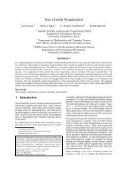
<strong>Texture</strong> <strong>Animation</strong> <strong>for</strong> <strong>Tensor</strong> <strong>Field</strong> <strong>Visualization</strong><br />
Louis Feng, Ingrid Hotz, Bernd Hamann, and Kenneth I. Joy<br />
Institute <strong>for</strong> Data Analysis and <strong>Visualization</strong> (IDAV)<br />
Department of Computer Science<br />
University of Cali<strong>for</strong>nia<br />
Davis, Cali<strong>for</strong>nia 95616<br />
{zfeng, ihotz}@ucdavis.edu, {hamann, joy}@cs.ucdavis.edu<br />
1. INTRODUCTION<br />
<strong>Tensor</strong> fields play an important role in many areas of engineering<br />
and physics. Due to their inherently large number of<br />
dimensions, it is not easy to visualize and understand these<br />
fields. There<strong>for</strong>e, it is important to visualize the data in a<br />
way that represents the physical meaning of the tensor field.<br />
In our application, we focus on stress and strain tensor fields.<br />
We use a texture-based method [3]. The texture is aligned<br />
to the eigenvector fields. The eigenvalues are encoded by the<br />
free parameters of the texture. To improve the impression<br />
of compression and stretching we animate this process. This<br />
approach requires one to control parameters locally, and <strong>for</strong><br />
continuous animation our approach requires a sequence of<br />
hierarchical sparse noise input images as basis <strong>for</strong> texture<br />
generation. Noise generation and sampling are closely related.<br />
Both are concerned with the placement of samples<br />
and their distributions. Many sampling algorithms, such as<br />
jittering, are often used directly to generate noise textures.<br />
Various techniques <strong>for</strong> generating samples and their properties<br />
have been explored extensively in the area of sampling<br />
and reconstruction theory to avoid aliasing problems. For a<br />
survey on sampling techniques, we refer to [2]. When sparse<br />
noise is used <strong>for</strong> texture generation, it is less important to determine<br />
the exact number of points to be generated. Rather,<br />
the size of the spots and spot distribution become more important.<br />
We specify the spots by size and density. Since<br />
sampling algorithms are mostly concerned with generating<br />
some predetermined number of samples, it is awkward to<br />
utilize existing sampling algorithms <strong>for</strong> our task. We have<br />
designed our algorithm to generate sparse noise with the<br />
following properties:<br />
• The noise is random, i.e., there are no inherent patterns.<br />
• The density of the noise can be controlled locally, but<br />
the total number of points is not important.<br />
• The distribution of the noise satisfies the Poisson-disk<br />
condition.<br />
• The algorithm can be applied to generate both 2D and<br />
3D textures.<br />
2. SPARSE NOISE<br />
The Poisson-disk distribution is a random pattern where no<br />
two disks overlap. One simple approach to generate random<br />
(a) (b) (c)<br />
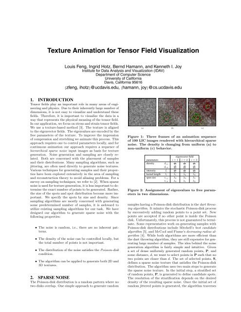
Figure 1: Three frames of an animation sequence<br />
of 100 LIC images rendered with hierarchical sparse<br />
noise. The density is changing from uni<strong>for</strong>m (a) to<br />
non-uni<strong>for</strong>m (c) behavior.<br />
eigenvector field<br />
parameters i =1 i =2 i =3<br />
density d i,j<br />
1 1 1<br />
λ2<br />
1<br />
d i,k λ2<br />
λ1<br />
1<br />
λ1<br />
1<br />
λ2<br />
λ1<br />
1<br />
λ1<br />
1<br />
λ3<br />
intensity I i<br />
1<br />
λ1<br />
kernel length l i λ 1 λ 2 λ 3<br />
spot size r i,j λ 2 λ 3 λ 1<br />
r i,k λ 3 λ 1 λ 2<br />
Figure 2: Assignment of eigenvalues to free parameters<br />
in two dimensions.<br />
samples having a Poisson-disk distribution is the dart throwing<br />
algorithm. It mimics the stochastic Poisson-disk process<br />
by successively adding random points to a point set. New<br />
points are accepted if no other point is inside the Poisson<br />
disk. Un<strong>for</strong>tunately, this process is not guaranteed to terminate.<br />
Some representative work on generating samples with<br />
Poisson-disk distributions include Mitchell’s best candidate<br />
algorithm [5], and McCool and Fiume’s decreasing radius algorithm<br />
[4]. While both algorithms are more efficient than<br />
the dart throwing algorithm, they are still expensive <strong>for</strong> generating<br />
large number of samples. The idea behind the noise<br />
generation algorithm is fairly simple and intuitive. Given<br />
a set of dense uni<strong>for</strong>mly generated random points, P, and<br />
some distance, d, we want to select points in P such that no<br />
two points are closer than d. The set of selected points, S,<br />
defines a sparse noise texture that satisfies the Poisson-disk<br />
distribution. The algorithm uses two main steps to generate<br />
the sparse noise texture. In the initial step, a stratified set<br />
of random points, P, is generated to define candidate spots.<br />
The resolution of the stratification depends on the desired<br />
density of the resulting sparse noise. Once the initial set of<br />
random jittered points is generated, the algorithm traverses
the set of points and decides whether each candidate spot<br />
should be inserted into S, the resulting texture. A candidate<br />
is selected when it satisfies the following criteria:<br />
• The point has not been checked previously, and<br />
• it does not overlap with any other selected spot in S.<br />
In our visualization, a set of hierarchical sparse noise texture<br />
is used to generate a sequence of slowly changing LIC<br />
images. It is important to maintain coherence from frame<br />
to frame in the animation. The changes between the frames<br />
should be minimal to avoid flickering. Given a set of initial<br />
stratified random points P, a sequence of n uni<strong>for</strong>m sparse<br />
noise textures generated from P is hierarchical, if the set of<br />
spots S i of each texture T i has the following relationship<br />
with subsequent textures:<br />
S 1 ⊆ S 2 ⊆ S 3 ⊆···S n−1 ⊆ S n ⊆ P (1)<br />
The textures should also maintain Poisson-disk distribution.<br />
It is fairly straight<strong>for</strong>ward to extend the sparse noise generation<br />
algorithm to generate textures with hierarchical characteristic.<br />
In more general cases, Equation 1 is only true<br />
locally.<br />
3. VISUALIZATION<br />
To motivate our approach, we briefly describe the tensor<br />
fields we are interested in, namely stress and (velocity) gradient<br />
tensor fields. The behaviors of stress tensor fields and<br />
gradient tensor fields are very similar. For a gradient field<br />
tensor and <strong>for</strong> stress and strain tensors positive eigenvalues<br />
lead to a separation of particles, or expansion of a probe.<br />
Eigenvalues equal to zero imply no change in distances, and<br />
negative eigenvalues indicate convergence of particles, or<br />
compression of the probe. Figure 2 shows the mapping from<br />
metric to texture parameters in two dimensions. A complete<br />
description of this metric can be found in [3].<br />
To visualize the change of distances and angles that represent<br />
the metric we use a texture that resembles the behavior<br />
of a piece of “fabric” when stretched or compressed and<br />
bent according to the metric. Large values of the metric,<br />
indicating large distances, are illustrated by a texture with<br />
low density or a stretched piece of fabric. We use a dense<br />
texture <strong>for</strong> small values of the metric. One can also think of<br />
a texture as a probe inserted into the tensor field. The texture<br />
is generated using LIC, a very popular method used <strong>for</strong><br />
vector field visualization. LIC blurs a noise image along the<br />
vector field or integral curves. Blurring results in a high correlation<br />
of the pixels along field lines, whereas in directions<br />
perpendicular to field curves almost no correlation appears.<br />
The resulting images lead to effective depictions of flow direction<br />
everywhere, even in a dense vector field. (LIC was<br />
introduced in 1993 by Cabral and Leedom [1], and there<br />
have been many extensions and improvements to make it<br />
faster [6] and more flexible.)<br />
We compute a LIC image <strong>for</strong> every eigenvector field to illustrate<br />
the eigendirections of a tensor field. To approximate<br />
the integral curves we use a Runge-Kutta method of fourth<br />
order, and the LIC image is computed using FastLIC as<br />
proposed in [6]. In each LIC image, the eigenvalues of every<br />
eigenvector field are integrated using the free parameters of<br />
the underlying noise image and the convolution. Eventually,<br />
we overlay all resulting LIC images to obtain the fabric-like<br />
texture. The free parameters of the input noise image determine<br />
the properties of the fabric. These parameters are:<br />
density, spot size, and color intensity of the spots. Considering<br />
these parameters, the standard white noise image is<br />
the noise image with maximum density, minimal spot size,<br />
and constant color intensity. It allows one to obtain a very<br />
good overall understanding of the field; its resolution is only<br />
limited by the pixel size. But it is not flexible enough to<br />
integrate the eigenvalues that represent fundamental field<br />
properties besides directionality. For this reason, we use<br />
sparse input images, with lower density and larger spot size<br />
even if we obtain a lower resolution. The connection of these<br />
parameters to the eigenvalues is described in Figure 1.<br />
4. RESULTS AND CONCLUSIONS<br />
We have evaluated our method <strong>for</strong> a data set generated via<br />
numerical finite element simulation. This data set represents<br />
a stress field where different load combinations were<br />
applied to a solid block. This data set is well-understood by<br />
engineers and there<strong>for</strong>e appropriate to evaluate our method.<br />
The simulation had been done <strong>for</strong> a ten-by-ten-by-ten grid.<br />
The tensor field resulting from the simulation is continuous<br />
inside each cell, but not on cell boundaries. This fact<br />
can also be observed in our images. The three-dimensional<br />
data set represents a block to which two <strong>for</strong>ces with opposite<br />
sign are applied. We have used one slice of the block<br />
and generated sparse textures based on local eigenvalues.<br />
Using our hierarchical non-uni<strong>for</strong>m sparse noise generation<br />
algorithm, we created a video showing a smooth animation<br />
of the changing process. Figure 1 shows the result after applying<br />
LIC to non-uni<strong>for</strong>m sparse textures. These images<br />
make possible a good visual segmentation of regions of compression<br />
and expansion. (Red indicates compression, white<br />
represents no change, and green refers to expansion.)<br />
5. REFERENCES<br />
[1] B. Cabral and L. Leedom. Imaging vector fields using<br />
line integral convolution. In Proceedings of SIGGRAPH<br />
93, pages 263–272, October 1993.<br />
[2] A. S. Glassner. Principles of Digital Image Synthesis.<br />
Morgan Kaufmann Publishers, Inc., 1995.<br />
[3] I. Hotz, L. Feng, H. Hagen, B. Hamann, B. Jeremic,<br />
and K. I. Joy. Physically based methods <strong>for</strong> tensor field<br />
visualization. In Proceedings of IEEE <strong>Visualization</strong><br />
2004, to appear, October 2004.<br />
[4] M. McCool and E. Fiume. Hierarchical poisson disk<br />
sampling distributions. In Proceedings of Graphics<br />
Interface, pages 94–105, 1992.<br />
[5] D. P. Mitchell. Spectrally optimal sampling <strong>for</strong><br />
distribution ray tracing. In Proceedings of the 18th<br />
annual conference on Computer Graphics and<br />
Interactive Techniques, pages 157–164. ACM Press,<br />
1991.<br />
[6] D. Stalling and H.-C. Hege. Fast and resolution<br />
independent line integral convolution. In Proceedings of<br />
SIGGRAPH 95, pages 149–256, October 1995.