Texture Animation for Tensor Field Visualization - CiteSeerX

the set of points and decides whether each candidate spot
should be inserted into S, the resulting texture. A candidate
is selected when it satisfies the following criteria:
• The point has not been checked previously, and
• it does not overlap with any other selected spot in S.
In our visualization, a set of hierarchical sparse noise texture
is used to generate a sequence of slowly changing LIC
images. It is important to maintain coherence from frame
to frame in the animation. The changes between the frames
should be minimal to avoid flickering. Given a set of initial
stratified random points P, a sequence of n uniform sparse
noise textures generated from P is hierarchical, if the set of
spots S i of each texture T i has the following relationship
with subsequent textures:
S 1 ⊆ S 2 ⊆ S 3 ⊆···S n−1 ⊆ S n ⊆ P (1)
The textures should also maintain Poisson-disk distribution.
It is fairly straightforward to extend the sparse noise generation
algorithm to generate textures with hierarchical characteristic.
In more general cases, Equation 1 is only true
locally.
3. VISUALIZATION
To motivate our approach, we briefly describe the tensor
fields we are interested in, namely stress and (velocity) gradient
tensor fields. The behaviors of stress tensor fields and
gradient tensor fields are very similar. For a gradient field
tensor and for stress and strain tensors positive eigenvalues
lead to a separation of particles, or expansion of a probe.
Eigenvalues equal to zero imply no change in distances, and
negative eigenvalues indicate convergence of particles, or
compression of the probe. Figure 2 shows the mapping from
metric to texture parameters in two dimensions. A complete
description of this metric can be found in [3].
To visualize the change of distances and angles that represent
the metric we use a texture that resembles the behavior
of a piece of “fabric” when stretched or compressed and
bent according to the metric. Large values of the metric,
indicating large distances, are illustrated by a texture with
low density or a stretched piece of fabric. We use a dense
texture for small values of the metric. One can also think of
a texture as a probe inserted into the tensor field. The texture
is generated using LIC, a very popular method used for
vector field visualization. LIC blurs a noise image along the
vector field or integral curves. Blurring results in a high correlation
of the pixels along field lines, whereas in directions
perpendicular to field curves almost no correlation appears.
The resulting images lead to effective depictions of flow direction
everywhere, even in a dense vector field. (LIC was
introduced in 1993 by Cabral and Leedom [1], and there
have been many extensions and improvements to make it
faster [6] and more flexible.)
We compute a LIC image for every eigenvector field to illustrate
the eigendirections of a tensor field. To approximate
the integral curves we use a Runge-Kutta method of fourth
order, and the LIC image is computed using FastLIC as
proposed in [6]. In each LIC image, the eigenvalues of every
eigenvector field are integrated using the free parameters of
the underlying noise image and the convolution. Eventually,
we overlay all resulting LIC images to obtain the fabric-like
texture. The free parameters of the input noise image determine
the properties of the fabric. These parameters are:
density, spot size, and color intensity of the spots. Considering
these parameters, the standard white noise image is
the noise image with maximum density, minimal spot size,
and constant color intensity. It allows one to obtain a very
good overall understanding of the field; its resolution is only
limited by the pixel size. But it is not flexible enough to
integrate the eigenvalues that represent fundamental field
properties besides directionality. For this reason, we use
sparse input images, with lower density and larger spot size
even if we obtain a lower resolution. The connection of these
parameters to the eigenvalues is described in Figure 1.
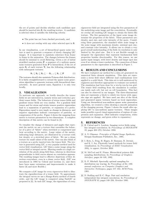
4. RESULTS AND CONCLUSIONS
We have evaluated our method for a data set generated via
numerical finite element simulation. This data set represents
a stress field where different load combinations were
applied to a solid block. This data set is well-understood by
engineers and therefore appropriate to evaluate our method.
The simulation had been done for a ten-by-ten-by-ten grid.
The tensor field resulting from the simulation is continuous
inside each cell, but not on cell boundaries. This fact
can also be observed in our images. The three-dimensional
data set represents a block to which two forces with opposite
sign are applied. We have used one slice of the block
and generated sparse textures based on local eigenvalues.
Using our hierarchical non-uniform sparse noise generation
algorithm, we created a video showing a smooth animation
of the changing process. Figure 1 shows the result after applying
LIC to non-uniform sparse textures. These images
make possible a good visual segmentation of regions of compression
and expansion. (Red indicates compression, white
represents no change, and green refers to expansion.)
5. REFERENCES
[1] B. Cabral and L. Leedom. Imaging vector fields using
line integral convolution. In Proceedings of SIGGRAPH
93, pages 263–272, October 1993.
[2] A. S. Glassner. Principles of Digital Image Synthesis.
Morgan Kaufmann Publishers, Inc., 1995.
[3] I. Hotz, L. Feng, H. Hagen, B. Hamann, B. Jeremic,
and K. I. Joy. Physically based methods for tensor field
visualization. In Proceedings of IEEE Visualization
2004, to appear, October 2004.
[4] M. McCool and E. Fiume. Hierarchical poisson disk
sampling distributions. In Proceedings of Graphics
Interface, pages 94–105, 1992.
[5] D. P. Mitchell. Spectrally optimal sampling for
distribution ray tracing. In Proceedings of the 18th
annual conference on Computer Graphics and
Interactive Techniques, pages 157–164. ACM Press,
1991.
[6] D. Stalling and H.-C. Hege. Fast and resolution
independent line integral convolution. In Proceedings of
SIGGRAPH 95, pages 149–256, October 1995.