Additive vs ultrametric: triangle inequality Additive vs ultrametric ...
Additive vs ultrametric: triangle inequality Additive vs ultrametric ...
Additive vs ultrametric: triangle inequality Additive vs ultrametric ...

You also want an ePaper? Increase the reach of your titles
YUMPU automatically turns print PDFs into web optimized ePapers that Google loves.
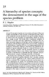
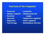
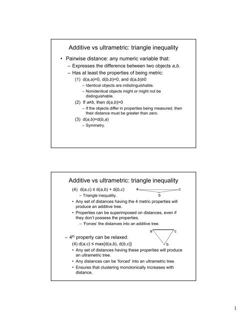
<strong>Additive</strong> <strong>vs</strong> <strong>ultrametric</strong>: <strong>triangle</strong> <strong>inequality</strong><br />
• Pairwise distance: any numeric variable that:<br />
– Expresses the difference between two objects a,b.<br />
– Has at least the properties of being metric:<br />
(1) d(a,a)=0, d(b,b)=0, and d(a,b)≥0<br />
– Identical objects are indistinguishable.<br />
– Nonidentical objects might or might not be<br />
distinguishable.<br />
(2) If a≠b, then d(a,b)>0<br />
– If the objects differ in properties being measured, then<br />
their distance must be greater than zero.<br />
(3) d(a,b)=d(b,a)<br />
– Symmetry.<br />
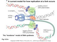
<strong>Additive</strong> <strong>vs</strong> <strong>ultrametric</strong>: <strong>triangle</strong> <strong>inequality</strong><br />
(4) d(a,c) ≤ d(a,b) + d(b,c) a<br />
– Triangle <strong>inequality</strong>.<br />
b<br />
• Any set of distances having the 4 metric properties will<br />
produce an additive tree.<br />
• Properties can be superimposed on distances, even if<br />
they don’t possess the properties.<br />
– ‘Forces’ the distances into an additive tree.<br />
a<br />
c<br />
–4 th property can be relaxed:<br />
(4) d(a,c) ≤ max{d(a,b), d(b,c)} d(bc)}<br />
b<br />
• Any set of distances having these properties will produce<br />
an <strong>ultrametric</strong> tree.<br />
• Any distances can be ‘forced’ into an <strong>ultrametric</strong> tree.<br />
• Ensures that clustering monotonically increases with<br />
distance.<br />
c<br />
1
Some commonly used distances<br />
• Euclidean distance:<br />
• Manhattan distance:<br />
• Mahalanobis distance:<br />
• Hamming distance between two strings of equal<br />
length: number of positions in which symbols are<br />
different (→ percent dissimilarity).<br />
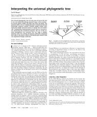
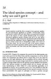
Ultrametric and additive trees for same data<br />
UPGMA<br />
7<br />
Neighbor-joining<br />
g<br />
6<br />
4<br />
5<br />
5<br />
7<br />
1<br />
4<br />
3<br />
2<br />
6<br />
1<br />
0.8<br />
0.7<br />
0.6 0.5 0.4 0.3<br />
Distance<br />
0.2<br />
0.1<br />
0<br />
2<br />
3<br />
Monotonically<br />
Increasing clustering<br />
2
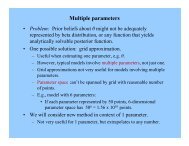
General procedure for<br />
hierarchical cluster analysis<br />
(1) Begin with N x N symmetric distance matrix.<br />
(2) Each object (taxon) initially considered to be a<br />
separate cluster.<br />
(3) Find two objects i and j separated by smallest<br />
distance.<br />
(4) Combine objects i and j into a new cluster, k.<br />
(5) Calculate distance between the new cluster and all<br />
other existing clusters.<br />
– Reduces size of the distance matrix.<br />
(6) Go to step 3. Continue until all objects have been<br />
merged into a single cluster.<br />
Cluster analysis<br />
• Methods differ according to (5) how distances are<br />
calculated between new cluster and all other<br />
existing clusters:<br />
– Single linkage:<br />
– Complete linkage:<br />
– UPGMA, WPGMA:<br />
3
Cluster analyses<br />
http://www.biomedcentral.com/1471-2105/9/90/figure/F5<br />
Distances are always estimates<br />
• Pairwise distance values are never exact:<br />
– Complete phylogenetic record of all<br />
genetic/phenotypic events would constitute set of<br />
distances that are completely:<br />
• <strong>Additive</strong>.<br />
• Mutually consistent across all taxa.<br />
– Observed distances are approximations:<br />
• Comprise ‘true’ distances, plus error.<br />
• Don’t display complete additivity and mutual<br />
consistency.<br />
– Additivity (metricity) and <strong>ultrametric</strong>ity are properties<br />
of a distance matrix.<br />
• Can be tested statistically.<br />
– Q: to what extent do methods recover ‘true’<br />
distances, in presence of error.<br />
4
UPGMA<br />
• UPGMA and other <strong>ultrametric</strong> methods assume<br />
that evolutionary rates have been constant:<br />
– Simulations show will work if rates are variable,<br />
but constant t on average (clocklike, =stationary).<br />
ti – But if rates are not clocklike, can give misleading<br />
results.<br />
– Estimation error can mimic effects of<br />
nonstationarity.<br />
<strong>Additive</strong> trees<br />
• Calculated in iterative fashion.<br />
– Several algorithms, most giving similar results.<br />
– Update placement of nodes rather than formation<br />
of clusters.<br />
• Rate uniformity not assumed.<br />
– Corrects original distances for unequal divergence<br />
among branches.<br />
• Least-squares and neighbor-joining trees<br />
guaranteed to recover true tree if distance matrix<br />
is an exact reflection of a tree.<br />
5
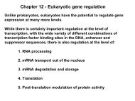
Phenetic <strong>vs</strong> patristic distances<br />
• Assessing agreement between tree and original<br />
distance matrix:<br />
– Patristic distance: predicted between two taxa by<br />
tree.<br />
• UPGMA: 2 x distance to nearest common node.<br />
• NJ: sum of horizontal branch lengths between taxa.<br />
UPGMA<br />
2<br />
Neighbor-joining<br />
7<br />
1<br />
6<br />
3<br />
3<br />
5<br />
2<br />
4<br />
1<br />
1<br />
0.8<br />
0.6 0.4<br />
Distance<br />
0.2<br />
7<br />
6<br />
0<br />
4<br />
5<br />
Correlations between<br />
phenetic and patristic distances<br />
• Ex: phenetic distances calculated from clocklike<br />
tree:<br />
– Add noise.<br />
– Calculate cophenetic correlation between phenetic<br />
and patristic distances.<br />
8<br />
r = 0.59<br />
UPGMA, 7 taxa<br />
8<br />
7.5<br />
r = 0.82<br />
Neighbor-joining tree, 7 taxa<br />
7<br />
Patristic distanc ce<br />
7<br />
6<br />
5<br />
4<br />
3<br />
ce<br />
Patristic distanc<br />
6.5<br />
6<br />
5.5<br />
5<br />
4.5<br />
4<br />
3.5<br />
4 4.5 5 5.5 6 6.5 7 7.5 8 8.5 9<br />
Original phenetic distance<br />
3 3.5 4 4.5 5 5.5 6 6.5 7 7.5 8<br />
Original phenetic distance<br />
6
Assessing confidence in trees<br />
• Two basic kinds of questions:<br />
(1) Is the overall tree “significant”, or significantly better<br />
than another tree<br />
• Permutation tests.<br />
• Frequency distributions of tree lengths.<br />
– E.g., g 1 statistic.<br />
• Likelihood and Bayesian scores.<br />
(2) Are particular parts of the tree “significant”<br />
• Bootstrapping.<br />
• Bayesian posterior probabilities.<br />
• Bremer support.<br />
Bootstrap<br />
• Bootstrap: general randomization procedure for estimating<br />
reliability of statistics:<br />
– Used primarily for estimating sampling distributions and<br />
associated confidence intervals.<br />
– Bootstrap p( (or bootstrapped) sample from a sample of N<br />
observations is a resample of those N observations with<br />
replacement.<br />
• Any particular observation might be sampled once, twice, or more<br />
often, or might be missed altogether.<br />
• Number of unique bootstrap samples: N N .<br />
• In practice, use a random set of bootstrap samples, sufficient to<br />
stabilize the values we’re trying to estimate.<br />
Original<br />
sample<br />
Bootstrapped resamples (of 46656 possible)<br />
1 1 2 6 5 4 5 6 3 6 4<br />
2 3 3 3 6 5 6 5 1 5 1<br />
3 4 1 2 3 1 6 4 5 1 5<br />
4 2 5 1 1 4 6 1 4 3 3<br />
5 4 1 4 6 1 5 4 5 6 2<br />
6 4 3 4 2 1 3 5 5 6 2<br />
7
Bootstrap<br />
Bootstrapped sampling distribution<br />
0.2<br />
cy<br />
Relative Frequen<br />
015 0.15<br />
0.1<br />
0.05<br />
0<br />
15 1.5 2 25 2.5 3 35 3.5 4 45 4.5 5 55 5.5<br />
Mean<br />
• Rationale and strong assumption: all observations are<br />
equivalent (i.e., independent replicates) and are<br />
representative off all possible observations that might<br />
have been sampled from the population.<br />
Bootstrapping trees<br />
• Very important topic in the theory and practice of<br />
phylogenetic inference.<br />
• Originally proposed for trees estimated by<br />
“parsimony” with discrete data (Felsenstein 1985).<br />
• Can be extended to all trees and networks:<br />
– Cladograms, dendrograms, phenograms, etc.<br />
8
Bootstrapping trees<br />
• Requires data matrix from which distance matrix<br />
is calculated:<br />
– Sample characters, with replacement, maintaining<br />
number of characters.<br />
• Bootstrapped sample, = pseudoreplicate.<br />
• Acts as a proxy for a true replicate from nature.<br />
– Convert pseudoreplicate data matrix to distance<br />
matrix.<br />
• For <strong>ultrametric</strong> and additive trees.<br />
– Construct tree, keep track of appearance of<br />
clusters (groups, clades, etc.).<br />
• Proportion of bootstrapped trees in which observed<br />
clusters occur.<br />
• Gives bootstrap support frequency (BSF).<br />
Original data matrix<br />
Bootstrapping trees<br />
Bootstrapped data matrix<br />
Characters<br />
Characters<br />
Taxon a b c d<br />
Taxon a a c c<br />
A 1 3 2 1 A 1 1 2 2<br />
B 2 4 5 1 B 2 2 5 5<br />
C 1 2 2 1 C 1 1 2 2<br />
D 2 1 3 3 D 2 2 3 3<br />
E 2 1 2 3 E 2 2 2 2<br />
• Assumes that characters are:<br />
– Independent (uncorrelated).<br />
– Equivalent (equally weighted).<br />
– Representative of an underlying pool of characters that<br />
might have been sampled.<br />
9
Bootstrapping trees<br />
Data matrix<br />
Pseudoreplicate<br />
data matrix<br />
Pseudoreplicate<br />
distance matrix<br />
Distance matrix<br />
Tree<br />
Record groups<br />
observed on tree<br />
Yes<br />
Continue<br />
No<br />
Calculate<br />
BSFs<br />
Pseudoreplicate<br />
tree<br />
Record whether<br />
observed<br />
groups are on<br />
pseudoreplicate<br />
tree<br />
Bootstrapped UPGMA and NJ trees<br />
from same random data<br />
0.52<br />
UPGMA<br />
0.98<br />
2<br />
1<br />
Neighbor-joining<br />
1.00<br />
0.64<br />
6<br />
7<br />
0.64<br />
3<br />
0.01<br />
3<br />
0.76<br />
5<br />
4<br />
0.01<br />
0.01<br />
1<br />
2<br />
1<br />
0.8<br />
0.6 0.4<br />
Distance<br />
0.96<br />
0.2<br />
7<br />
6<br />
0<br />
4<br />
5<br />
10
Common interpretations of<br />
bootstrap support frequencies<br />
• Probability that the cluster (clade) will be observed on<br />
repeated sampling of many characters from the<br />
underlying pool of characters.<br />
• Confidence limit on a cluster.<br />
• Level of “significance” of a cluster.<br />
• Probability that a given cluster is a “real” group.<br />
• General measure of support for a given cluster.<br />
Assessing the “significance” of a<br />
bootstrap support frequency<br />
• Minimum-50% (majority consensus) rule.<br />
• Gestalt 70% rule (Hillis & Bull 1993).<br />
• 1-P rule (Felsenstein & Kishino 1993).<br />
• However:<br />
– None of these rules is adequate.<br />
– All can be misleading.<br />
11
Expected BSFs per<br />
hundred bootstrap iterations<br />
(by simulation)<br />
0.7<br />
1.5<br />
6.7<br />
A<br />
B<br />
C<br />
6.7<br />
1.5<br />
1.5<br />
6.7<br />
D<br />
E<br />
F<br />
G<br />
H<br />
I<br />
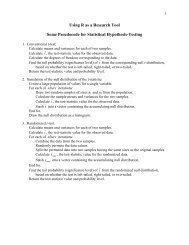
Other methods for modeling distance matrices<br />
Cluster analysis<br />
methods<br />
Ultrametric<br />
2.5<br />
<strong>Additive</strong><br />
2<br />
1.5<br />
3<br />
1<br />
5<br />
0.5<br />
4<br />
1<br />
2<br />
0<br />
4<br />
3<br />
5<br />
2<br />
1<br />
Distance matrix<br />
1 2 3 4 5<br />
1 0.00 1.41 2.45 2.45 2.83<br />
2 1.41 0.00 2.45 3.16 2.45<br />
3 2.45 2.45 0.00 1.41 1.41<br />
4 245 2.45 316 3.16 141 1.41 000 0.00 245 2.45<br />
5 2.83 2.45 1.41 2.45 0.00<br />
Data<br />
matrix<br />
Characters<br />
Taxa a b c<br />
1 1 2 1<br />
2 2 1 1<br />
3 3 3 2<br />
4 2 4 2<br />
5 3 2 3<br />
Correlation matrix<br />
a b c<br />
a 1.00 0.16 0.79<br />
b 0.16 1.00 0.37<br />
c 0.79 0.37 1.00<br />
PCo2 (34.5% %)<br />
Dim2<br />
PC2 (29.4%)<br />
1<br />
0.5<br />
Ordination<br />
methods<br />
Principal coordinates<br />
0<br />
-0.5<br />
-1<br />
1<br />
0.5<br />
0<br />
-0.5<br />
-1<br />
-1.5<br />
4<br />
2<br />
3<br />
5<br />
-1 -0.5 0 0.5 1 1.5<br />
PCo1 (60.6%)<br />
Multidimensional scaling<br />
1<br />
0.5<br />
0<br />
-0.5<br />
-1<br />
1<br />
5<br />
-1.5 -1 -0.5 0 0.5 1<br />
Dim1<br />
Principal components<br />
1<br />
2<br />
-1.5 -1 -0.5 0 0.5 1 1.5<br />
PC1 (64.5%)<br />
4<br />
3<br />
1<br />
3<br />
2<br />
4<br />
5<br />
12
Principal coordinates analysis (PCoA)<br />
• Eigenanalysis method:<br />
– Decomposes information in the distance matrix into a set of<br />
orthogonal axes:<br />
• Axes = principal coordinates.<br />
• Orthogonal = statistically independent.<br />
– Principal coordinates:<br />
• PCo1 accounts for the maximum information in the distance matrix.<br />
• PCo2 accounts for the maximum residual information in the<br />
distance matrix, independent of PCo1.<br />
• PCo3 accounts for the maximum residual information in the<br />
distance matrix, independent of both PCo1 and PCo2.<br />
• Etc.<br />
– For an N×N distance dsta matrix, ,there eeae are N principal pa coordinates.<br />
• The full set of N principal coordinates accounts for all of the<br />
information in the distance matrix.<br />
– Observations (taxa) are projected onto the axes to give<br />
projection scores, which can be plotted with scattergrams.<br />
Principal coordinates analysis (PCoA)<br />
5<br />
Distance matrix<br />
1 2 3 4 5<br />
1 0.00 1.41 2.45 2.45 2.83<br />
2 1.41 0.00 2.45 3.16 2.45<br />
3 2.45 2.45 0.00 1.41 1.41<br />
4 2.45 3.16 1.41 0.00 2.45<br />
5 2.83 2.45 1.41 2.45 0.00<br />
<strong>Additive</strong><br />
4<br />
PCo2 (34.5%)<br />
1<br />
0.5<br />
0<br />
-0.5<br />
-1<br />
4<br />
3<br />
-1 -0.5 0 0.5 1 1.5<br />
PCo1 (60.6%)<br />
1<br />
2<br />
3<br />
5<br />
2<br />
1<br />
13
Multidimensional scaling (MDS)<br />
• Not an eigenanalysis method:<br />
– Information in distance matrix is not decomposed.<br />
• Points representing observations (taxa) are<br />
‘squeezed’ into 1D, 2D, or 3D… space.<br />
– Placed into space so that interpoint distances<br />
reconstruct original distances as much as possible.<br />
• Metric and nonmetric (monotonic) versions.<br />
– Axes are arbitrary, and points can be arbitrarily rotated.<br />
– Amount of distortion measured as ‘stress’.<br />
• Observations (taxa) are projected onto the axes to<br />
give projection scores, which can be plotted with<br />
scattergrams.<br />
Multidimensional scaling (MDS)<br />
Stress = 0.27<br />
Distance matrix<br />
1 2 3 4 5<br />
1 0.00 1.41 2.45 2.45 2.83<br />
2 1.41 0.00 2.45 3.16 2.45<br />
3 2.45 2.45 0.00 1.41 1.41<br />
4 2.45 3.16 1.41 0.00 2.45<br />
5 2.83 2.45 1.41 2.45 0.00<br />
Dim2<br />
1<br />
0.5<br />
0<br />
-0.5<br />
-1<br />
2<br />
1<br />
3<br />
4<br />
<strong>Additive</strong><br />
4<br />
-1.5 15<br />
-1.5 -1 -0.5 0 0.5 1<br />
Dim1<br />
5<br />
3<br />
5<br />
2<br />
1<br />
14
Principal components analysis (PCA)<br />
• Eigenanalysis method, but based on correlation or covariance<br />
matrix:<br />
– Decomposes information in the correlation matrix into a set of<br />
orthogonal axes:<br />
• Axes = principal p components.<br />
• Orthogonal = statistically independent.<br />
– Principal components:<br />
• PC1 accounts for the maximum information in the distance matrix.<br />
• PC2 accounts for the maximum residual information in the distance<br />
matrix, independent of PC1.<br />
• PC3 accounts for the maximum residual information in the distance<br />
matrix, independent of both PC1 and PC2.<br />
• Etc.<br />
– For an N×N correlation matrix, there are N principal<br />
components.<br />
• The full set of N principal components accounts for all of the<br />
information in the distance matrix.<br />
– Observations (taxa) are projected onto the axes to give<br />
projection scores, which can be plotted with scattergrams.<br />
Principal components analysis (PCA)<br />
4<br />
1<br />
Correlation matrix<br />
a b c<br />
a 1.00 0.16 0.79<br />
b 0.16 1.00 0.37<br />
c 0.79 0.37 1.00<br />
PC2 (29.4%)<br />
0.5<br />
0<br />
1<br />
3<br />
-0.5<br />
<strong>Additive</strong><br />
-1<br />
2<br />
5<br />
-1.5 -1 -0.5 0 0.5 1 1.5<br />
PC1 (64.5%)<br />
4<br />
3<br />
5<br />
2<br />
1<br />
15