Metropolis-Hastings algorithm
Metropolis-Hastings algorithm
Metropolis-Hastings algorithm

You also want an ePaper? Increase the reach of your titles
YUMPU automatically turns print PDFs into web optimized ePapers that Google loves.
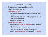
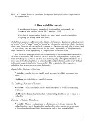
Multiple parameters<br />
• Problem: Pi Prior blif beliefs about θ might not be adequately<br />
represented by beta distribution, or any function that yields<br />
analytically solvable posterior function.<br />
• One possible solution: grid approximation.<br />
– Useful when estimating one parameter, e.g. θ.<br />
– However, typical models involve multiple parameters, not just one.<br />
– Grid approximations not very useful for models involving multiple<br />
parameters.<br />
– Parameter space can’t be spanned by grid with reasonable number<br />
of points.<br />
– E.g., model with 6 parameters:<br />
• If each parameter represented by 50 points, 6-dimensional<br />
i parameter space has 50 6 = 1.56 x 10 10 points.<br />
• We will consider new method in context of 1 parameter.<br />
– Not very useful for 1 parameter, but extrapolates to any number.
• Initial i assumptions:<br />
Monte Carlo approach<br />
– Prior distribution is specified by function (continuous or discrete) that is<br />
easily evaluated (by computer):<br />
• If specify θ, then p(θ) is easily determined.<br />
– Likelihood function, p(D | θ), can be determined for any specified values of<br />
D and θ.<br />
– (Actually, all that is required is that the product of the prior and the<br />
likelihood be easily determined.)<br />
• Method produces an approximation of the posterior distribution, p(θ | D):<br />
– Provides large number of θ values sampled from the posterior distribution.<br />
– Can be used to estimate:<br />
• Mean, median, standard ddeviation of posterior.<br />
• Credible HDI regions.<br />
• Etc.<br />
• Example of Monte Carlo method.
Monte Carlo approach<br />
• Basic goal lin Bayesian inference: describe posterior distribution<br />
ib i<br />
over the parameters.<br />
• Monte Carlo approach:<br />
– Sample large number of representative points from posterior.<br />
– From points, calculate descriptive statistics.<br />
• E.g., consider beta(θ | a, b) distribution:<br />
ib ti<br />
– Mean and standard deviation can be analytically derived.<br />
• Expressed exactly in terms of parameters a and b.<br />
– Cumulative probability distribution (cdf, qbeta in R) can be<br />
computed.<br />
• Used to determine credible intervals.<br />
• But: suppose didn’t know analytical formulas or cdf.
• Use a spinner:<br />
Monte Carlo approach<br />
– Marked on circumference with possible θ values.<br />
– Biased to point at θ values exactly according to a beta(θ | a, b)<br />
distribution.<br />
<br />
<br />
beta |1,1 :<br />
– Spin 1000s of times, record the values.<br />
– Calculate statistics (mean, standard deviation, etc.) and percentiles.<br />
– Should closely approximate properties of the ‘underlying’<br />
distribution.
<strong>Metropolis</strong>-<strong>Hastings</strong> <strong>algorithm</strong><br />
• Imagine a politician visiting a string of islands:<br />
– Wants to visit each island a number of times proportional to its<br />
population.<br />
– Doesn’t know how many islands there are.<br />
– Each day: might move to a new neighboring island, or stay on current<br />
island.<br />
• Develops simple heuristic to decide which way to move:<br />
– Flips a fair coin to decide whether to move to east or west.<br />
– If the proposed island has a larger population than the current island,<br />
moves there.<br />
– If the proposed island has a smaller population than the current island,<br />
moves there probabilistically, based on uniform spinner:<br />
• Probability of moving depends on relative population sizes:<br />
P<br />
proposed<br />
pmove<br />
<br />
P<br />
current<br />
• End result: probability that politician is on any one of the islands<br />
exactly matches the relative proportion of the island.
<strong>Metropolis</strong>-<strong>Hastings</strong> <strong>algorithm</strong><br />
• E.g., have 7 islands (θ = 1–7)<br />
with relative populations given<br />
by P(θ).<br />
• Initial island (θ = 4) chosen<br />
randomly (or centered).<br />
• Each ‘day’ corresponds to one<br />
time increment.<br />
• Trajectory path is a random walk<br />
on a grid.<br />
• One possible instance of a<br />
trajectory:<br />
Resulting frequency distribution<br />
Random walk<br />
Target distribution
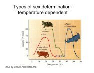
<strong>Metropolis</strong>-<strong>Hastings</strong> <strong>algorithm</strong><br />
• Probability of being at position θ, as a function of time t, when<br />
y g p , ,<br />
<strong>Metropolis</strong> <strong>algorithm</strong> is applied to target distribution (lower right):
<strong>Metropolis</strong>-<strong>Hastings</strong> <strong>algorithm</strong><br />
• Summary of <strong>algorithm</strong>:<br />
– Currently at position<br />
.<br />
current<br />
– Range of possible proposed moves is the proposal distribution<br />
(=trial distribution).<br />
• Sampled uniformly.<br />
• Island example: 2 values with 50-50 probabilities.<br />
– Given a proposed p move, must decide to accept or reject it.<br />
proposed<br />
• Based on value of target distribution at relative to value<br />
of target distribution at current<br />
.<br />
• If target value is > current value, move.<br />
• If target value is < current value, move with probability<br />
P <br />
proposed <br />
p<br />
move<br />
<br />
P <br />
current<br />
<br />
• Combined movement rule (=jumping rule): move with probability<br />
p<br />
move<br />
<br />
<br />
min <br />
P<br />
<br />
proposed<br />
P <br />
<br />
,1<br />
<br />
<br />
<br />
<br />
<br />
current
<strong>Metropolis</strong>-<strong>Hastings</strong> <strong>algorithm</strong><br />
• What we must be able to do:<br />
– Select a random value from the proposal distribution (to<br />
create θ proposed ).<br />
– Evaluate the target distribution at any proposed position θ (to<br />
calculate P(θ proposed ) / P(θ current ) .<br />
– Select a random value from a uniform distribution (to make a<br />
move according to p move ).<br />
• Can then do something indirectly than can’t necessarily to<br />
directly: generate random samples from the target distribution.<br />
ib i
<strong>Metropolis</strong>-<strong>Hastings</strong> <strong>algorithm</strong><br />
• Note: target distribution ib i does not need to be normalized.<br />
– Based on ratio: P(θ proposed ) / P(θ current ) .<br />
– Useful when target distribution P(θ) is a posterior distribution<br />
p D| p .<br />
proportional to <br />
pD|<br />
p<br />
<br />
Bayes’ rule:<br />
p<br />
<br />
|<br />
D<br />
<br />
p D<br />
<br />
p | D<br />
pD|<br />
p<br />
<br />
– Need only evaluate the product p D| p , not the separate<br />
likelihoods and priors.<br />
– By evaluating p D<br />
| <br />
p<br />
<br />
,<br />
can generate random representative<br />
values from the posterior distribution.<br />
– Don’t need to evaluate evidence, pD.<br />
• Can do Baysian inference with rich and complex models.
• Algorithm named after:<br />
<strong>Metropolis</strong>-<strong>Hastings</strong> <strong>algorithm</strong><br />
– Nicholas <strong>Metropolis</strong> (et al., 1953), physicist who was first author<br />
(of 5) on paper that proposed it. (Other coauthors actually did<br />
more work.)<br />
– W. Keith <strong>Hastings</strong> (1970), mathematician who extended to the<br />
general case.<br />
• Commonly used Markov-chain Monte Carlo (MCMC) method.<br />
• Why Markov<br />
• Markov process: process in which the probability of passing<br />
from a current state to another particular state is constant, and<br />
depends d only on the current state.<br />
• Markov chain: probabilistic instance of a Markov process based<br />
on a random walk through the probabilistic decisions.
MCMC methods<br />
• Markov chain Monte Carlo methods:<br />
– Class of <strong>algorithm</strong>s for sampling from a probability distribution.<br />
– Based on constructing a Markov chain.<br />
– Desired distribution is the equilibrium distribution.<br />
• State of Markov chain after many steps then used as a sample of<br />
the desired distribution.<br />
– Quality of the sample improves as the number of steps increases.<br />
• Difficult problem is to determine how many steps are needed to<br />
converge to the stationary distribution within an acceptable<br />
error.<br />
– A good <strong>algorithm</strong> will have rapid mixing: the stationary<br />
distribution is reached quickly starting from an arbitrary position.<br />
– <strong>Metropolis</strong>-<strong>Hastings</strong> <strong>algorithm</strong> has rapid-mixing gproperties.<br />
p
General <strong>Metropolis</strong>-<strong>Hastings</strong> <strong>algorithm</strong><br />
• Specific procedure just described was special case:<br />
– Discrete positions (θ);<br />
– One dimension;<br />
– Moves that proposed one position left or right.<br />
• General <strong>algorithm</strong> applies to:<br />
– Continuous values;<br />
– Any number of dimensions;<br />
– More general proposed distributions.<br />
• Essentials are same as for special case:<br />
– Have some target distribution, P(θ), over a multidimensional<br />
continuous parameter space.<br />
– Would like to generate representative samples.<br />
– Must be able to find value of P(θ) for any candidate value of θ.<br />
– Distribution P(θ) does not need to be normalized, merely non-negative.<br />
– Typical Bayesian application: P(θ) is product of likelihood and prior.
General <strong>Metropolis</strong>-<strong>Hastings</strong> <strong>algorithm</strong><br />
• Sample values from target distribution generated by taking a random<br />
walk through the multidimensional parameter space.<br />
– Begins at arbitrary point, specified by user, where P(θ) is non-zero.<br />
– At each time step:<br />
• Move to new position in parameter space is proposed.<br />
• Decide whether or not to accept move to new position.<br />
– Proposal distributions can be of various forms.<br />
• Goal is to efficiently explore regions of parameter space where P(θ)<br />
has greatest mass.<br />
• Simplest case: proposal distribution is normal, centered on current<br />
position.<br />
• Proposed move will typically ybe near present position, with probability<br />
of more distant positions decreasing with distance:<br />
0.4<br />
0.35<br />
0.3<br />
025 0.25<br />
P()<br />
0.2<br />
0.15<br />
0.1<br />
0.05<br />
0<br />
-3 -2 -1 0 1 2 3
General <strong>Metropolis</strong>-<strong>Hastings</strong> <strong>algorithm</strong><br />
• Sample values from target distribution generated by taking a random<br />
walk through the multidimensional parameter space.<br />
– At each time step:<br />
• Having generated proposed new position, decision made whether to<br />
accept or reject it based on movement rule:<br />
p<br />
move<br />
<br />
<br />
<br />
min <br />
P<br />
<br />
proposed<br />
P <br />
<br />
,1<br />
<br />
<br />
<br />
<br />
current<br />
<br />
• Random number r generated from uniform interval [0, 1].<br />
• If r is between 0 – p move , move is accepted.<br />
– Process repeated.<br />
– In the long run: positions visited by the random<br />
walk will closely approximate the target distribution.<br />
θ 2<br />
θ 1
Visualization of <strong>Metropolis</strong> <strong>algorithm</strong> in 1D<br />
• R code for excellent visualization i of the <strong>Metropolis</strong> <strong>algorithm</strong><br />
for a 1D problem at:<br />
– http://www.r-bloggers.com/visualising-the-metropolis-hastings<strong>algorithm</strong>/<br />
– Minor modifications, code saved as: Chivers_ms_viz.R<br />
<strong>Metropolis</strong><br />
s-<strong>Hastings</strong><br />
Trace<br />
rm(x, target_mu, target_sd)<br />
dnor<br />
-3 -2 -1 0 1 2 3<br />
x
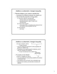
Efficiency, “burn-in”, and convergence<br />
• If proposal ldistribution ib i is narrow relative to target distribution ib i ,<br />
will take a long time for random walk to cover the distribution.<br />
– Algorithm will not be efficient: takes too many steps to accumulate<br />
a representative sample.<br />
– Particular problem if initial position of random walk is in region of<br />
target distribution that is flat and low.<br />
• Random walk moves only slowly away from starting position<br />
into denser region.<br />
– Unrepresentative starting gposition can lead to low efficiency even<br />
if proposal distribution isn’t narrow.<br />
• Solution: early steps of random walk are excluded from portion<br />
of Markov chain considered to be representative of target<br />
distribution.<br />
– Excluded initial steps: burn-in period.
Efficiency, “burn-in”, and convergence<br />
• Efficiency also decreases if proposal distribution is too broad:<br />
– If too broad, proposed positions are far away, away from main<br />
mass of distribution.<br />
– Probability bilit of accepting a move will be small.<br />
– Random walk rejects too many proposals before accepting one.<br />
• Simulation for 1–64 dimensional target distribution:<br />
ciency<br />
% Effic<br />
Stdev of proposal distribution
Efficiency, “burn-in”, and convergence<br />
• Even after random walk lkhas meandered dfor a while, can’t be<br />
sure that it’s really exploring the main regions of the target<br />
distribution.<br />
– Especially if target distribution is complex over many dimensions.<br />
– But don’t know what target distribution looks like.<br />
• Various methods available to assess convergence of random<br />
Various methods available to assess convergence of random<br />
walk.