Novel Definition of Cost Function for Camera Calibration using ...

Journal of Academic and Applied Studies 

Vol. 2(6) June 2012, pp. 1- 10 

Available online @ www.academians.org 

ISSN1925-931X 

Novel Definition of Cost Function for Camera 

Calibration using Vanishing Point Theorem 

Razieh Zamani, Saeed Tousizadeh, Reyhaneh Kardehi Moghaddam 

Islamic Azad University, Mashhad Branch 

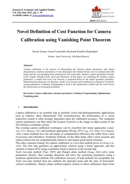
Abstract 

Camera calibration is the process of determining the internal camera parameters and optical 

characteristics (intrinsic parameters). It also determines the relation between the two dimensional (2D) 

image and the corresponding three dimensional (3D) real points. Intrinsic camera parameters include: 

Focal Length, Principal Point, and Lens Distortion. In this paper, for estimating the intrinsic camera 

parameters, a simple and novel cost function is proposed based on the spatial geometry principles. 

Minimizing the proposed cost function, results in an accurate and simultaneous estimation of intrinsic 

camera parameters. Nonlinear Programming is used as the optimization method and the result shows 

the effectiveness of our proposed method. 

Keywords: Camera calibration, intrinsic parameters, Nonlinear Programming, Optimization, 

Vanishing point. 

I. Introduction 

Camera calibration is an essential step in machine vision and photogrammetric applications 

such as robotics, three dimensional (3D) reconstructions; the performance of a vision 

inspection system is often strongly dependent upon the calibration accuracy. The computed 

camera parameters can then relate the location of pixels in the image to object points in the 

3D reference coordinate system. 

The existing camera calibration techniques can be classified into linear approaches (Abdel- 

Aziz, 1971; Okamoto, 1981) and nonlinear approaches (Wong, 1975; Faig, 1975; Sobel, 1974, Paquette, 

1990). Linear methods have the advantage of computational efficiency but suffer from a lack 

of accuracy and robustness. Nonlinear methods, on the other hand, offer a more accurate and 

robust solution but are computationally intensive and require good initial estimates 

The other common strategy for camera calibration is a two-step method given in (Weng et al., 

1992). The first step generates an approximate solution using a linear approach, and this 

solution is improved by using a nonlinear iterative process in the second step. 

Tsai's two-step method (Tsai, 1987) and Zhang's plane method (Zhang, 2000) solve some 

parameters linearly, then consider distortion and solve the remaining parameters using a 

nonlinear optimization method; The calibration accuracy of both methods are acceptable, but 

Tsai's two-step method does not calibrate the principal point and the ratio of horizontalvertical 

coordinates. Zhang’s plane method requires camera to shoot calibration object from 

1


Vol. 2(6) June 2012, pp. 1- 10 


ISSN1925-931X 

various angles. Reference (Wei xing and Feng, 2006) proposes a linear calibration method basing 

on coplanar, but the method ignores the lens distortion and the calibration accuracy is low. 

The first step utilizing linear approaches is a key to the success of two-step methods. 

Approximate solutions provided by the linear techniques must be good enough for the 

subsequent nonlinear techniques to correctly converge. Being susceptible to noise in image 

coordinates, the existing linear techniques are, however, notorious for their lack of robustness 

and accuracy (Wang and Xu, 1996). In ref (Haralick et al., 1989) shows that when the noise level 

exceeds a knee level or the number of points is below a knee level, these methods become 

extremely unstable and the errors diverge. 

The use of more points can help alleviate this problem. However, fabrication of more control 

points often proves to be difficult, expensive, and time-consuming. For applications with a 

limited number of control points, e.g., close to the required minimum number, it is 

questionable whether linear methods can consistently and robustly provide well enough 

initial guesses for the subsequent nonlinear procedure to correctly converge to the optimal 

solution. Another problem is that almost all nonlinear techniques employed in the second step 

use variants of conventional optimization techniques. They therefore all inherit well known 

problems plaguing these conventional optimization methods, namely, poor convergence and 

susceptibility to getting trapped in local extremum. If the starting point of the algorithm is not 

well chosen, the solution can diverge, or get trapped at a local minimum. This is especially 

true if the objective function landscape contains isolated valleys or broken ergodicity. 

In this paper we introduced a cost function based on the spatial geometry principles. In this 

method Nonlinear Programming is used as the optimization tool. The innovation of the 

proposed method is the estimation simultaneity of all intrinsic camera parameters using the 

cost function that includes all intrinsic camera parameters and normalized projected points of 

the real world. Result shows an accurate and feasible estimation of intrinsic camera 

parameters. 

II. 

Nonlinear Programming 

Nonlinear programming (NLP) is the process of determining unknown parameters of system 

for minimizing an objective function subject to nonlinear system equations and some equal or 

non equal conditions. The NLP problems have the common following form: 

min f(x) 

xεX 

s. t. g(x) ≤ 0 

X ⊆ R n 

where X is a subset of R n x , and f : x → R, g: X → R n g 

and f is the objective 

function.g i (x) ≤ 0, i = 1,..., n g , are inequality constraints, and i (x) = 0, i = 1,……., n ,are 

constraints. Note also that the set X typically includes lower and upper bounds on the 

variables; the reason for separating variable bounds from the other inequality constraints is 

that they can play a useful role in some algorithms, i.e., they are handled in a specific way. 

2


Vol. 2(6) June 2012, pp. 1- 10 


ISSN1925-931X 

Easily we can say that the NLP is the problem of finding a feasible point x ∗ such that f(x) ≥ 

f(x ∗ ) where x ∗ is a feasible solution, which satisfies all constraints. for each feasible point x 

needless to say, a NLP problem can be stated as a minimization problem, and the inequality 

constraints can be written in the form can be written in the form g(x) ≥ 0. 

III. 

Camera Model 

Earlier camera calibration techniques usually employed a perfect pinhole camera model. 

p w : A point in a three-dimensional (3D) space in front of the camera. 

P w = 

P wx 

P wy 

P wz 

(1) 

p c : Coordinates of p w in camera system coordinates. 

P c = 

P cx 

P cy 

P cz 

(2) 

x ∗ ,y ∗ are the coordinates of the principal point in the 

Image plane: 

x ∗ 

y ∗ = 

f 

P cz 

P cx 

P cy 

(3) 

The relation between the real world coordinate (3D coordinate) and camera system 

coordinate is as follows: 

Where 

e : canonical center coordinate 

M cw : Camera orientation 

P w =M cw P C + e , M cw = 

u 1 v 1 w 1 

u 2 v 2 w 2 (4) 

u 3 v 3 w 3 

P C =M wc (P w - e) , M cw T = M wc (5) 

IV. 

Marker projection on the Image Plane Procedure 

We assume m is a point in the camera system coordinate 

3


Vol. 2(6) June 2012, pp. 1- 10 


ISSN1925-931X 

x m 

x m 

x m 

(6) 

n is the normalized coordinates of m based on pinhole camera model 

x n 

y n 

= 

x m zm 

y m zm 

(7) 

r is defined as follows: 

By applying lens distortion model to n, 

d is obtained. 

r 2 = x n 

2 

+ y n 

2 

(8) 

x d 

y d 

= (1 + k 1 r 2 + k 2 r 4 ) x n 

y n 

(9) 

After applying lens distortion model by applying camera model matrix, the final pixel position 

related to the projection of m in camera image plane, calculated as follows: 

x p 

y p 

1 

= 

f x αf x x R 

0 f y y R 

0 0 1 

x d 

y d 

1 

(10) 

The above square matrix (K) is called Calibration Matrix. 

The constraints are obtained from equations (11) and (12). 

f x .x n . (1+k 1 .r 2 +k 2 .r 4 ) + x R -x p =0 (11) 

f y .y n . (1+k 1 .r 2 +k 2 .r 4 ) + y R -y p =0 (12) 

V. Objective Function 

Earlier than introducing the objective function it is necessary to explain the concept of vanishing 

point comprehensibly. 

A. Vanishing point of a line 

4


Vol. 2(6) June 2012, pp. 1- 10 


ISSN1925-931X 

The vanishing point of a line is a point on the image plane that is obtained by intersecting the image 

plane with a ray parallel to the world line and passing through the camera centre. 

The perspective geometry that gives rise to vanishing points is illustrated in Figure 1. In this figure, 

the point C is the camera centre and plane S is the image plane. Vector d is a vector with direction 

of the line D. The vanishing point, v, of the line D with direction d, is the intersection of the image 

plane (plane S) with a ray parallel to d through C (camera centre). Thus a vanishing point of a line 

depends only on the direction of the line, not on its position. Consequently a set of parallel lines 

have a unique vanishing point, as illustrated in Figure 1. For example image of infinite railway 

lines, are converging lines, and their image intersection is the vanishing point for the direction of 

the railway. Therefore parallel world lines are projected as converging lines, and their image 

intersection is the vanishing point of them. 

X 

X’ 

C 

V’ 

V 

D 

X 1 X 2 X 3 

X 4 X 

(a) 

A 

d 

X(λ) 

d\ 

V 

X(λ) 

C 

S 

(b) 

Figure. 1. Vanishing point formation, (a) Plane to line camera. The points X i , i= 1,... ,4 are equally 

spaced on the world line, but their spacing on the image line monotonically decreases. In the limit 

5


Vol. 2(6) June 2012, pp. 1- 10 


ISSN1925-931X 

X ∞ the world point is imaged at x = v on the vertical image line, and at x' = v' on the inclined 

image line. Thus the vanishing point of the world line is obtained by intersecting the image plane 

with a ray parallel to the world line through the camera centre C. (b) 3-space to plane camera. The 

vanishing point, v, of a line with direction d is the intersection of the image plane with a ray 

parallel to d through C. 

B. Objective function introduction 

Consider the rectangle ABCD in 3D world and quadrilateral (A ’ B ’ C ’ D’) as the image of 

rectangle ABCD on the image plane of the camera and suppose that this camera is calibrated 

perfectly. As shown in the fig. 1, lines AB and CD are parallel; therefore their image intersection 

(point s) is vanishing point of AB and CD. Also AD and BC are parallel and their image 

intersection (point t) is vanishing point of AD and BC. Consequently based on vanishing point 

definition, os is parallel with AB and CD and ―ot‖ is parallel with AD and BC in 3D world. t and s 

are the vanishing points of orthogonal lines, therefore inner product of os and ot is zero.(figure 2) 

A 

B 

Real object in 3D 

D 

C 

Accurate image on 

the image plane 

B’ 

v 

Image plane 

Vanishing point of AB and CD 

A’ 

s 

D’ 

C’ 

u 

90 

o 

t 

Vanishing point of AD and BC 

w 

Figure. 2. Marker projections on image plane and the cost function based on spatial geometry rules 

Assume camera is not calibrated correctly and suppose that instead of correct image (A’B’C’D’), 

quadrilateral A‖B‖C‖D‖ imaged on the image plane of the camera, so the intersection of A‖B‖ and 

C‖D‖ (point s’) is not vanishing point of AB and CD ,s’ and s aren’t coincident certainly. Also AD 

and BC are parallel and their image intersection (point t’ that is the intersection of A‖D‖ and C‖B‖) 

is not vanishing point of AD and BC t’ and t aren’t coincident certainly. So os’ and ot’ lines isn’t 

orthogonal therefore inner product os’ by ot’ isn’t zero. (figure 3) 

6


Vol. 2(6) June 2012, pp. 1- 10 


ISSN1925-931X 

Non accurate image 

on the image plane 

B‖ 

v 

Image plane 

A‖ 

D‖ 

C‖ 

u 

s’ 

t’ 

o 

Figure. 3. Marker projections on image plane and the cost function based on spatial geometry rules 

w 

In this paper inner product is defined as objective function, if camera is calibrated correct inner 

product os by ot, which must be minimized. It’s obvious that if the camera is calibrated properly, s’ 

and t’ are coincident on s and t respectively, therefore inner product which must be minimized. 

VI. 

Experimental Results 

According to the information provided by the camera manufacturer, values of the intrinsic camera 

parameters are as follows: f x = f y =720, x R = 320, y R = 240, α = 0 and k 1 = k 2 = 0. 

(f x , f y ) focal length, (x R , y R ) Principal point coordinate, (k 1 , k 2 ) lens distortion and α is skew 

coefficient that here we assume it is equal to zero. 

With assumption of knowing the intrinsic parameters, we can calculate the position of points on the 

image plane. (x p , y p ) 

Based on the inverted camera model (k −1 ), x d and y d are estimated. 

x d 

y d1 = 

1 

f x 

0 − x R 

0 

1 

f y 

f x 

− y R 

f y 

0 0 1 

x p 

y p 

1 

(13) 

7


Vol. 2(6) June 2012, pp. 1- 10 


ISSN1925-931X 

According to equation (14) related to lens distortion parameters, the equation between distorted 

points (x d , y d ) and normalized points (x n , y n ) corresponding to the projection of the markers on the 

image plane is as follows: 

x n 

y n 

= 

1 

(1+ k 1 r 2 + k 2 r 4 ) 

x d 

y d 

(14) 

Where equation (8) shows the relation between (x n , y n ) and r in the above equation. 

The objective function depends on a set of (x n , y n ) on the image plane that are calculated from 

equation (14), and also other intrinsic camera parameters. Minimizing this objective function by 

Nonlinear Programming results in an accurate intrinsic camera parameters estimation. 

Table I shows the results of the estimation by Nonlinear Programming based on various noise 

values, where k 1 and k 2 are constant and k 1 = k 2 = 0. 

TABLE I: estimation results by Nonlinear Programming based on various noise values, where k 1 

and k 2 are constant and k 1 = k 2 = 0. 

Noise 

level 

0 

0.05 

0.1 

0.15 

0.2 

fx 

719.9556 

722.545 

716.8452 

710.225 

709.3547 

fy 

721.0308 

723.922 

729.652 

717.5412 

712.5698 

XR 

319.0014 

321.084 

318.9502 

326.379 

329.5421 

YR 

240.6515 

238.7119 

239.3665 

246.6462 

245.2248 

Table II, shows the results of the estimation by Nonlinear Programming based on various noise 

values, where k 1 and k 2 are constant and k 1 = 0.01, k 2 = 0.001. 

TABLE II: estimation results by Nonlinear Programming based on various noise values, where k 1 

and k 2 are constant and k 1 = 0.01, k 2 = 0.001 

Noise 

level 

fx 

fy 

XR 

YR 

0 

0.05 

0.1 

0.15 

0.2 

718.5489 

717.2259 

710.561 

710.668 

709.5414 

724.5625 

727.5487 

718.548 

707.894 

710.5796 

317.895 

326.8457 

315.6511 

315.6874 

310.5833 

243.784 

245.5694 

236.455 

234.8875 

231.8541 

Table III shows the results of the estimation by Nonlinear Programming based on various noise 

values, where k 1 and k 2 are variables.This means that lens distortion is considered here. 

8


Vol. 2(6) June 2012, pp. 1- 10 


ISSN1925-931X 

TABLE III: estimation results by Nonlinear Programming based on various noises values, where k 1 

and k 2 are variables. This means that lens distortion is considered here. 

Pe 

fx 

fy 

XR 

YR 

K1 

K2 

0 

718.0318 

723.248 

320.8841 

241.3108 

-3165e-7 

631e-8 

0.05 

722.9632 

725.1154 

319.0064 

241.0171 

6353e-7 

5032e-8 

0.1 

724.4826 

724.8421 

317.2564 

238.3443 

117e-8 

165e-9 

0.15 

729.2331 

715.7809 

325.1152 

245.1457 

365e-7 

7528e-8 

0.2 

728.907 

729.1426 

310.5887 

246.2149 

713e-7 

5064e-8 

VII. 

Conclusion 

The cost function is obtained by vanishing Point Theorem which is one of the spatial geometry 

principles also Nonlinear programming is used for minimizing the objective function. Calibration 

on a sample camera based on the proposed objective function resulted an accurate and feasible 

estimation of intrinsic camera parameters. 

9


Vol. 2(6) June 2012, pp. 1- 10 


ISSN1925-931X 

References 

Abdel-Aziz YI and. Karara HM. (1971) ―Direct linear transformation into object space coordinates in close-range 

photogrammetry,‖ in Proc. Symp. Close-Range Photogrammetry, Urbana-Champaign, IL, pp 1-18. 

Faig W. (1975) ―Calibration of close-range photogra mmetry systems: Mathematical formulation,‖ Photogram. Eng. 

Remote Sens., Vol(41), pp 1479–1486. 

Haralick RM, Joo H, Lee C, Zhang X., Vaidya V, and Kim M. (1989) ―Pose estimation from corresponding point data,‖ 

IEEE Trans. Syst., Man, Cybern., Vol(19), pp 1426–1446. 

Okamoto A. (1981) ―Orientation and construction of models—Part i: The orientation problem in close-range 

photogrammetry,‖ Photogramm. Eng. Remote Sens., Vol(5), pp 1437-1454. 

Paquette LR. Stampfler,W, Devis A., and Caelli TM. (1990) ―A new camera calibration method for robotic vision,‖ in 

Proceedings SPIE: Closed Range Photogrammetry Meets Machine Vision, Zurich, Switzerland, pp 656–663. 

Sobel I. (1974) ―On calibrating computer controlled cameras for perceiving 3d scenes,‖ Artif. Intell, Vol(5), pp 1437– 

1454. 

Tsai RY. (1987),"A versatile camera calibration technique for high accuracy 3D machine vision metrology using offthe-shelf 

TV cameras and lenses", IEEE Journal of Robotics and Automation, Vol(U), noA, pp 323-334. 

Wang X, and Xu G. (1996) ―Camera parameters estimation and evaluation in active vision system,‖ Pattern Recognit., 

Vol(29), no. 3, pp 439–447. 

Wei xing Z, and Feng X. (2008) "Simple camera parameters calibration technique based on coplanar camera", 

Computer Engineering and Applications, Vo1(44), no.2, pp 86-88. 

Weng J, Cohen P, and Herniou M. (1992) ―Camera calibration with distortion models and accuracy evaluation‖, IEEE 

Transcations on Pattern Analysis and Machine Intelligence, Vol(10), pp 965-980. 

Wong KW. (1975) ―Mathematical formulation and digital analysis in closerange photogrammetry,‖ Photogramm. Eng. 

Remote Sens., Vol(41), no.11, pp 1355–1373. 

Zhang ZY, (2000) "A flexible new technique for camera calibration", IEEE Transactions on Pattern Analysis and 

Machine Intelligence, VoI(22), no, ll, pp 1330-1334. 

10

Novel Definition of Cost Function for Camera Calibration using ...

You also want an ePaper? Increase the reach of your titles

Delete template?

Save as template?