controller parameters by using a decoupling filter

The transfer functions of the G 11 and G 22 of the decoupled
system can now be presented in equation (21) and (22).
G
22
4
−3,264⋅10
G11
=
0.05916s+
1
4 0.11063s+
1
= 4,94⋅10 0.05916s + 1
(21)
(22)
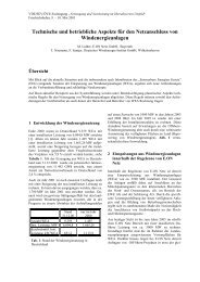
Figure 6 shows the bode chart of the transfer function of
-G 11 (blue) and G 22 (green).
If the controller provides a lower gain crossover
frequency than ω f
the DC current control is delayed.
Hence the gain was chosen to K p = -0,006 in order to
exceed this limiting value for the open loop gain
crossover frequency and to adapt the control direction
with the negative sign. Consequently the DC current
controller has the following structure:
C
11
1+
0.05916s
= − 0.006 . (25)
0.05916s
Figure 7 shows the bode chart of the closed loop system
and it can be easily seen that the system is speeded up.
Figure 6: Bode chart of the transfer function -G 11 (blue) and
G 22 (green)
G 11 shows delay first order behaviour with a negative gain.
The negative sign of G 11 is not taken into account for
further studies since the control direction is simply adapted
with a negative sign in the controller gain. G 22 is a PDT1
element.
The next two sections will show how control design is
applied for the mathematically separated systems G 11 and
G 22 .
A. Control design for G 11
Since the transfer functions G 11 is already pretty fast due to
its large gain crossover frequency, it is sufficient to use a
PI controller, which will handle the steady-state accuracy.
The equation of a PI controller is shown in (23).
1+ T s
C K T
N
11
=
p
(23)
N
s
Where K p is the gain and T N is the time constant of the PI
controller. The time constant of the PI controller is chosen
in order to eliminate the pole in the transfer function G 11 .
The gain of the controller has to be chosen in order to
guarantee a certain dynamic behaviour. A limiting factor is
the firing delay of 60° on average. The firing frequency
can be calculated as shown in equation (24).
Figure 7: Bode chart of the closed loop system C 11·G 11
B. Control design for G 22
As already mentioned G 22 is described by a PDT2
element, which is similar to an all-pass filter. This means,
that all frequencies are barely damped. Therefore also
PDT2 controller can be deployed where the equation is
presented in (26).
( 1+
TN
s)
s1 ( + s)
C22 = Kp
T
N T
V
(26)
The time constants T N and T V of the PDT2 controller are
chosen in order to eliminate the pole in the transfer
function G 22 and the zero respectively. Hence the closed
loop transfer function is described by a delay first order
element. Therefore the gain of the PDT2 controller can
be chosen in order to guarantee a fast dynamic response
as well as a sufficiently damped transient behavior. The
gain was set to K p = 0,006. Hence the appropriate PDT2
controller C 22 can be presented in equation (27).
C
22
1+
0.05916s
= 0,006 0.05916s 1 0.11063s
( + )
(27)
360°⋅50 Hz
ωf
= 2π
= 1885rad/ sec
60°
(24)
The bode plot of the closed loop system is shown in
Figure 8. It can also be seen that the system is speeded
up.