controller parameters by using a decoupling filter

International Conference on Renewable Energies and Power Quality (ICREPQ’13)
Bilbao (Spain), 20 th to 22 th March, 2013
Renewable Energy and Power Quality Journal (RE&PQJ)
ISSN 2172-038 X, No.11, March 2013
A novel approach to select HVDC - controller parameters by using a decoupling
filter
C. Hahn 1 , A. Müller 1 and M. Luther 1
1 Chair of Electrical Energy Systems
University of Erlangen – Nuremberg
Konrad-Zuse-Straße 3-5, 91052 Erlangen (Germany)
Phone/Fax number: +49 9131 8523446, e-mail: Christoph.Hahn@ees.fau.de, Annatina-Mueller@web.de,
Matthias.Luther@ees.fau.de
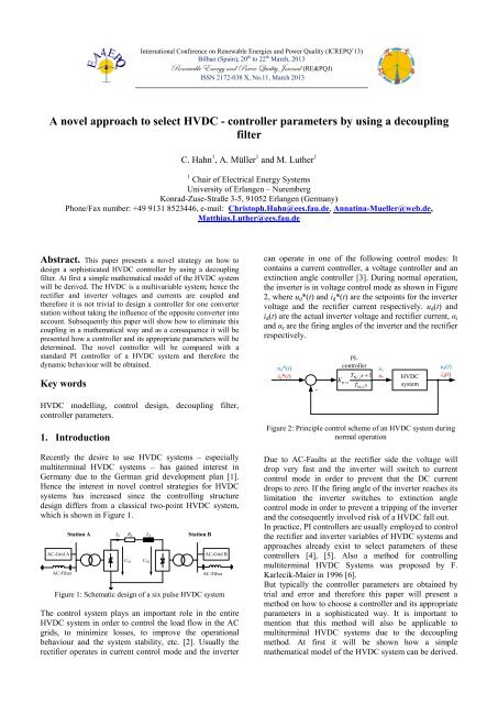
Abstract. This paper presents a novel strategy on how to
design a sophisticated HVDC controller by using a decoupling
filter. At first a simple mathematical model of the HVDC system
will be derived. The HVDC is a multivariable system; hence the
rectifier and inverter voltages and currents are coupled and
therefore it is not trivial to design a controller for one converter
station without taking the influence of the opposite converter into
account. Subsequently this paper will show how to eliminate this
coupling in a mathematical way and as a consequence it will be
presented how a controller and its appropriate parameters will be
determined. The novel controller will be compared with a
standard PI controller of a HVDC system and therefore the
dynamic behaviour will be obtained.
Key words
HVDC modelling, control design, decoupling filter,
controller parameters.
1. Introduction
Recently the desire to use HVDC systems – especially
multiterminal HVDC systems – has gained interest in
Germany due to the German grid development plan [1].
Hence the interest in novel control strategies for HVDC
systems has increased since the controlling structure
design differs from a classical two-point HVDC system,
which is shown in Figure 1.
AC-Grid A
AC-Filter
Station A
Id
Rd
Ud1
Ld
Ud2
Station B
AC-Grid B
AC-Filter
Figure 1: Schematic design of a six pulse HVDC system
The control system plays an important role in the entire
HVDC system in order to control the load flow in the AC
grids, to minimize losses, to improve the operational
behaviour and the system stability, etc. [2]. Usually the
rectifier operates in current control mode and the inverter
can operate in one of the following control modes: It
contains a current controller, a voltage controller and an
extinction angle controller [3]. During normal operation,
the inverter is in voltage control mode as shown in Figure
2, where u d *(t) and i d *(t) are the setpoints for the inverter
voltage and the rectifier current respectively. u d (t) and
i d (t) are the actual inverter voltage and rectifier current, α i
and α r are the firing angles of the inverter and the rectifier
respectively.
u d *(t)
i d *(t)
-
K
PIcontroller
T
Nr,i
p r,
i
TNr,
i
s+
1
s
α i
α r
HVDC
system
u d (t)
i d (t)
Figure 2: Principle control scheme of an HVDC system during
normal operation
Due to AC-Faults at the rectifier side the voltage will
drop very fast and the inverter will switch to current
control mode in order to prevent that the DC current
drops to zero. If the firing angle of the inverter reaches its
limitation the inverter switches to extinction angle
control mode in order to prevent a tripping of the inverter
and the consequently involved risk of a HVDC fall out.
In practice, PI controllers are usually employed to control
the rectifier and inverter variables of HVDC systems and
approaches already exist to select parameters of these
controllers [4], [5]. Also a method for controlling
multiterminal HVDC Systems was proposed by F.
Karlecik-Maier in 1996 [6].
But typically the controller parameters are obtained by
trial and error and therefore this paper will present a
method on how to choose a controller and its appropriate
parameters in a sophisticated way. It is important to
mention that this method will also be applicable to
multiterminal HVDC systems due to the decoupling
method. At first it will be shown how a simple
mathematical model of the HVDC system can be derived.

Afterwards the control design process based on this
mathematical model will be shown and the performance of
the developed controller will be presented.
2. Modelling of the HVDC system
As already mentioned in the previous section, the first step
is to analyse the HVDC system in order to obtain a simple
mathematical model. At first the transmission equation can
be directly obtained from Figure 1.
d I
IR+ L = U −U
dt
d
d d d d1 d2
The voltage drop along the DC line, between the rectifier
and inverter, can be replaced by equation (2) and (3),
which show the correlation between the DC voltages U d1
and U d2 , the DC current I d , the firing angle α r , the
extinction angle γ i and the corresponding phase to phase
voltages of the AC grids U nr and U ni [3].
(1)
Ud1 = B 3 2 U 3
nr
cosα
r
− B XCrI d
π
π
(2)
Ud 2
= B 3 2 U 3
n i
cosγ
i
− B XCiI d
π
π
(3)
Where X Cr and X Ci are the short-circuit reactances of the
AC grids. As the extinction angle γ i is not an actuating
variable of the system it can be replaced with its
appropriate firing angle α i . For a six-pulse converter the
constant B is fixed to one (B = 1). Inserting equations (2)
and (3) in equation (1) yields equation (4).
d Id
IR
d d
+ Ld
=
d t
3 2 3
= ( U cosα
+ U cosα
) − ( X
π
π
+ X ) I
nr r n i i Cr Ci d
This equation describes a nonlinear system and needs to be
linearized. This can be done through use of the Taylor
series decomposition method, where the differential terms
with orders greater than one are neglected. After the
linearization the equation can be transferred to the Laplace
domain.
(4)
I
d
(s)
2U
sinα
α (s)
π π
s Ld + Rd + XCr + XCi
3
3
nr 0 r
= −
r
−
G11
2U
ni
sinα0i
π
d
+
d
+
Cr
+
Ci
3
−
αi
(s).
π
s L R X X
3
G12
The next step is to deduce the relation between the firing
angles and the inverter side DC voltage U d2 . Therefore
equation (3) will be linearized and transformed to the
Laplace domain.
(6)
Ud 2
(s) = 3 2 U 3
n iαi (s)sin α0i − XCiI d
(s) (7)
π
π
Replacing the DC current I d in equation (7) with (6)
yields equation (8).
Ud2(s)
=
π π
s Ld + Rd + X
3 2
Cr
= U
3 3
ni
sin α0i αi
(s)
π
π π
s Ld + Rd + XCr + XCi
3 3
G22
3 2
X
Ci
− U
nr
sin α0 r
αr
(s)
π
π π
s Ld + Rd + XCr + XCi
3 3
G21
Summarizing equation (6) and (8) yields in the transfer
matrix G.
⎛ Id (s) ⎞ ⎛G11 G12 ⎞⎛αr
(s) ⎞
⎜ ⎟=
⎜ ⎟⎜ ⎟
⎝Ud2(s)
⎠ ⎝G21 G22 ⎠⎝αi
(s)
⎠
As the transfer matrix shows, the model is a two-variable
system where all the variables are influenced by each
other. The structure of the system is shown in Figure 3.
α r
G11
G
Id
(8)
(9)
3 2
Id (s) Rd + s LI
d d
(s) = − ( Unrαr (s)sinα0 r
+
π
3
+ Un iαi (s)sin α0i ) − ( XCr + XCi ) Id
(s)
π
α 0r and α 0i are the operating points of the firing angle of the
rectifier and the inverter respectively. Hence the transfer
function of the DC current can be obtained:
(5)
G12
G21
α i
Ud2
G22
Figure 3: Structure of the simplified HVDC Model

It is not possible to design an appropriate controller for
such a system due to the fact that both, actuating and
control variables, are coupled. Applying a so called
decoupling filter to the system makes it possible to
consider the coupled system mathematically decoupled
[7]. The filter compensates the influence of the secondary
diagonal elements G 12 and G 21 . Its matrix is shown in
equation (10).
F ⎛F11 F12
⎞
= ⎜ ⎟
⎝F21 F
(10)
22 ⎠
The structure of the system with the applied filter and the
controllers C 11 and C 22 is shown in Figure 4.
F
G
= − F ,
(13)
12
12 22
G11
F
G
= − F .
(14)
21
21 11
G22
The direct influences from the input to the output, shown
in Figure 4, shall remain and therefore the equations can
be presented.
( )
( )
I = ∆IC FG + FG
(15)
d d 11 21 12 11 11
U = ∆U C FG + FG (16)
d 2 d 2 22 12 21 22 22
Comparing those to the decoupled structure scheme,
shown in Figure 5, yields in the following equations:
Idref
-
∆Id
C11
F11
α r
G11
Id
G = FG + FG
(17)
11 21 12 11 11 ,
G = FG + FG
(18)
22 12 21 22 22 .
F12
F21
G12
G21
Inserting equation (13) in (17) and equation (14) in (18)
respectively and solving the equations for F 11 or F 22
respectively one obtains equation (19).
Ud2ref
-
∆Ud2
C22
F22
α i
G22
Ud2
F
GG
11 22
= F =
GG − GG
11 22
11 22 12 21
(19)
Figure 4: Structure of the HVDC system with inculded filter and
controllers
The controllers C 11 and C 22 and its parameters are a degree
of freedom and can be selected in order to guarantee a
certain dynamic behaviour of the HVDC system. Selecting
the filter parameters in the right way, the system can be
considered completely decoupled and has a structure as
shown in Figure 5.
-
∆Id
Idref α r
Id
C11
G11
Hence the decoupling filter matrix is given through
equation (20).
GG
⎛
⎜
⎜
1
11 22
11
F =
(20)
GG ⎜
⎟
11 22
− GG
12 21
G21
⎜−
⎝ G
22
G
−
G
The system can now be considered as a mathematically
uncoupled system and control design can be applied
much easier.
1
12
⎞
⎟
⎟
⎟
⎠
Ud2ref ∆Ud2
α i
Ud2
C22
G22
-
Figure 5: Structure of the HVDC system with the applied
decoupling filter
The first step in the creation of the filter matrix is to reveal
the undesired influence of the DC current I d on the inverter
end DC voltage U d2 and to zero it in.
( )
( )
∆ IC FG + FG =
(11)
d 11 21 22 11 21
0
∆ U C FG + FG = (12)
d 2 22 12 11 22 12
0
Solving these equations yields in the following expressions
for the secondary diagonal elements of the decoupling
filter:
3. Control Design
For designing a sophisticated controller for the HVDC
system, a simple test network was build up in MATLAB ®
Simulink ® with some standard values for Back-to-Back
HVDC systems from [4] and [8], shown in Table I.
Table I - HVDC Values
U nr
200 kV
U ni
200 kV
X cr
0,7 Ω
X ci
0,7 Ω
R d
0,1 Ω
L d 0,085H
U d2ref
255 kV
I dref
3000 A
α 0r 10°
α 0i 160°

The transfer functions of the G 11 and G 22 of the decoupled
system can now be presented in equation (21) and (22).
G
22
4
−3,264⋅10
G11
=
0.05916s+
1
4 0.11063s+
1
= 4,94⋅10 0.05916s + 1
(21)
(22)
Figure 6 shows the bode chart of the transfer function of
-G 11 (blue) and G 22 (green).
If the controller provides a lower gain crossover
frequency than ω f
the DC current control is delayed.
Hence the gain was chosen to K p = -0,006 in order to
exceed this limiting value for the open loop gain
crossover frequency and to adapt the control direction
with the negative sign. Consequently the DC current
controller has the following structure:
C
11
1+
0.05916s
= − 0.006 . (25)
0.05916s
Figure 7 shows the bode chart of the closed loop system
and it can be easily seen that the system is speeded up.
Figure 6: Bode chart of the transfer function -G 11 (blue) and
G 22 (green)
G 11 shows delay first order behaviour with a negative gain.
The negative sign of G 11 is not taken into account for
further studies since the control direction is simply adapted
with a negative sign in the controller gain. G 22 is a PDT1
element.
The next two sections will show how control design is
applied for the mathematically separated systems G 11 and
G 22 .
A. Control design for G 11
Since the transfer functions G 11 is already pretty fast due to
its large gain crossover frequency, it is sufficient to use a
PI controller, which will handle the steady-state accuracy.
The equation of a PI controller is shown in (23).
1+ T s
C K T
N
11
=
p
(23)
N
s
Where K p is the gain and T N is the time constant of the PI
controller. The time constant of the PI controller is chosen
in order to eliminate the pole in the transfer function G 11 .
The gain of the controller has to be chosen in order to
guarantee a certain dynamic behaviour. A limiting factor is
the firing delay of 60° on average. The firing frequency
can be calculated as shown in equation (24).
Figure 7: Bode chart of the closed loop system C 11·G 11
B. Control design for G 22
As already mentioned G 22 is described by a PDT2
element, which is similar to an all-pass filter. This means,
that all frequencies are barely damped. Therefore also
PDT2 controller can be deployed where the equation is
presented in (26).
( 1+
TN
s)
s1 ( + s)
C22 = Kp
T
N T
V
(26)
The time constants T N and T V of the PDT2 controller are
chosen in order to eliminate the pole in the transfer
function G 22 and the zero respectively. Hence the closed
loop transfer function is described by a delay first order
element. Therefore the gain of the PDT2 controller can
be chosen in order to guarantee a fast dynamic response
as well as a sufficiently damped transient behavior. The
gain was set to K p = 0,006. Hence the appropriate PDT2
controller C 22 can be presented in equation (27).
C
22
1+
0.05916s
= 0,006 0.05916s 1 0.11063s
( + )
(27)
360°⋅50 Hz
ωf
= 2π
= 1885rad/ sec
60°
(24)
The bode plot of the closed loop system is shown in
Figure 8. It can also be seen that the system is speeded
up.

)
Time/sec.
Figure 9: Power-up process of the HVDC system with a) the
classical controller b) the decoupling filter controller
Figure 8: Bode chart of the closed loop system C 22·G 22
4. Results
In this section the results of the aforementioned control
design process will be presented. Therefore the novel
approach will be compared with a classical HVDC control
scheme. This comparison will include normal operating
conditions as well as operation during fault conditions.
The classical HVDC controller consists of two controllers,
a PI controller at the rectifier end for the DC current and a
PI controller at the inverter end for the DC voltage.
Therefore standard HVDC PI parameters are considered
and shown in Table II.
Table II: Parameters of standard HVDC PI controllers [4]
PI at rectifier side PI at inverter side
K p T N K p T N
0,4 0,015 sec. 0,2 0,02 sec
This behaviour differs from the predicted delay first
order; the reason is a simplification in the system model.
As already mentioned the HVDC is a nonlinear system
due to the sinusoidal dependence of the system variables
on the firing angle and also due to the firing delay of 60°
on average [9]. This firing delay is equal to a dead-time
element. During this interval of 60° the HVDC is not
capable to interact and therefore the overshoot arises. The
transfer function of such a dead-time element can be
described as follows.
F (s) e − T t s
t
= (28)
Another positive impact is the smoothness of the firing
angels, which implies that there aren’t any additional
filters for the DC current and voltage values in the
controlling software required; the firing angles are
presented in Figure 10.
A. No fault operation
The first simulation shows a power-up process of the
HVDC system with the different controllers deployed; it is
presented in Figure 9.
It is very conspicuous that the decoupling filter controller
is much faster than the classical controller. It reaches its
reference level for the DC voltage approximately four
times faster than the classical controller. In order to
achieve this goal one has to accept overshoots in the DC
current.
a)
Time/sec.
b)
a)
Time/sec.
Time/sec.
Figure 10: Firing angles of the HVDC system with a) the
classical controller b) the decoupling filter controller

B. Operation during AC faults
The AC fault applied to the HVDC system is a 50%
voltage jump at the AC side of the inverter; it is presented
in Figure 11.
Time/sec.
Figure 11: 50 % voltage jump from t = 0.5 sec to t = 0.7 sec
applied to the inverter AC side of the HVDC system with a) the
classical controller b) the decoupling filter controller
During the AC fault, the rectifier firing angle decreases
and is controlled to its average reference value. The DC
current drops to zero. Applying the classical control the
current overshoot after the fault is much higher than
applying the decoupling filter controller. The decoupling
filter reacts much faster than the classical controller and
reaches its reference level much earlier regarding the DC
voltage.
5. Conclusion
a)
Time/sec.
b)
In this paper a novel approach for the selection of HVDC
controller parameters was presented. First the
mathematical modelling of an HVDC was shown, thus it
was revealed that the HVDC is a coupled system due to
the firing of the rectifier influences the DC current and the
DC voltage at the inverter; the same applies for the firing
of the inverter respectively and was presented in Figure 3.
Accordingly a decoupling filter was designed for the
HVDC system and it was shown, that the system can be
considered as mathematically uncoupled.
This method offers the possibility to select the HVDC
controllers and their parameters in a sophisticated way
that takes the HVDC parameters of the mathematical
model into account. Therefore an appropriate controller
for each HVDC system can be designed; unlike the
parameters of classical controllers which were obtained
by trial and error.
The controller was tested in a realistic environment and it
was shown, that the developed controller operates well
and that it behaves even better under certain operating
conditions than the classical HVDC controller.
It was also shown that the curves of the firing angles are
very smooth, therefore no additional software smoothing
filters would be necessary in the controller like it is
necessary for the classical controller.
References
[1] O. Feix, R. Obermann, M. Strecker and A. Brötel,
“German grid development plan, (Netzentwicklungsplan
Strom)“, German Transmission System Operators, Berlin,
Germany, August 2012 (in German).
[2] L. Ni and Y. Tao, “Parameter Optimization of the Control
and Regulating System of Gezhouba-shanghai HVDC
Project”, Power System Technology, No.3, pp.26-31, Aug.
1989.
[3] V. Crastan and D. Westermann, “Electrical power supply
III, (Elektrische Energieversorgung III)”, Springer
publishing, Berlin Heidelberg, Germany, 2012 (in
German).
[4] F. Yang and Z. Xu, “An approach to Select PI Parameters
of HVDC Controllers”, Power Engineering Society
General Meeting, Montreal, Québec, Canada, June 2006.
[5] A. E. Hammad, “Stability and Control of HVDC and AC
Transmissions in Parallel”, IEEE Transactions on Power
Delivery, Vol. 14, No. 4, October 1999.
[6] F. Karlecik-Maier, “A New Closed Loop Control Method
for HVDC Transmission”, IEEE Transactions on Power
Delivery, Vol. 11, No. 4, October 1996.
[7] O. Föllinger, “Control Engineering, (Regelungstechnik)”,
Hüthig publishing, Heidelberg, Germany, 1994 (in
German).
[8] T. Rae, E. Boje, G. D. Jennings and R. G. Harley,
“Controller structure and design of firing angle controllers
for (unit connected) HVDC systems”, 4 th IEEE Africon
Conference, Stellenbosch, South Africa, September 1996.
[9] C. Hahn, M. Weiland, G. Herold, “Control design for a
power electronic based fault current limiter (FCL)”,
International Conf. on Renewable Energies and Power
Quality (ICREPQ), Santiago de Compostela (Spain), 2012.