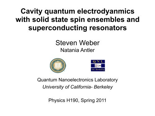
Cavity quantum electrodyanmics with solid state spin ensembles ...

Cavity quantum electrodyanmics
with solid state spin ensembles and
superconducting resonators
Steven Weber
Natania Antler
Quantum Nanoelectronics Laboratory
University of California- Berkeley
Physics H190, Spring 2011

Cavity quantum electrodyanmics
with solid state spin ensembles and
superconducting resonators
Steven Weber
Natania Antler
Quantum Nanoelectronics Laboratory
University of California- Berkeley
Physics H190, Spring 2011

-atom in a cavity
Cavity QED

Cavity QED
-atom in a cavity
-ensemble of spins
coupled to a superconducting
resonator

Motivation
- Collective coupling strong coupling
- Long coherence times
- Swap quantum state between a superconducting
qubit and the spin ensemble quantum memory
-Access new regimes of cavity QED

Outline
- Cavity QED
- Superconducting resonators
- Coupling NV centers to a resonator
- Outlook

Cavity QED
CHAPTER 2. CAVITY QUANTUM ELECTRODYNAMICS 35
γ ⊥
from quantum optics group at CalTech
g
κ
T transit
Figure 2.1: A two level atom interacts with the field inside of ahighfinessecavity. Theatom
coherently interacts with the cavity at a rate, g. Alsopresentaredecoherenceprocessesthatallow
the photon to decay at rate κ, theatomtodecayatrateγ ⊥ into modes not trapped by the cavity,
and the rate at which the atom leaves the cavity, 1/T . To reach the strong coupling limit the
interaction strength must larger than the rates of decoherence g>κ, γ ⊥ , 1/T transit .
leakage or absorption by the cavity results in a photon decay rate, κ, sometimesexpressedinterms
of the quality factor Q = ω r /κ. Often, and particularly in circuit QED, κ is set by the desired
transparency of the mirrors to allow some light to be transmitted to a detector as a means of
probing the dynamics of the system. In the absence of other decay mechanisms, the radiative decay
of the atom can be completely described in terms of the coherent interaction with the cavity and
decay of cavity photons (which are measured). This very well modeled (and often slow) decay makes
cavity QED a good test-bed for studying quantum measurement and open systems [Mabuchi2002].

Cavity QED
CHAPTER 2. CAVITY QUANTUM ELECTRODYNAMICS 35
ystemforstudyingtheinteractionbetweenmatter and light is
a dipole coupling with a cavity, described by aharmonicoscillato
γ ⊥
from quantum optics group at CalTech
g
κ
T transit
e Fig. 2.1). The coherent behavior of this coupled system is descri
iltonian [Walls2006]:
Figure 2.1: A two level atom interacts with the field inside of ahighfinessecavity. Theatom
coherently interacts with the cavity at a rate, g. Alsopresentaredecoherenceprocessesthatallow
Jaynes-Cummings Hamiltonian
the photon to decay at rate κ, theatomtodecayatrateγ ⊥ into modes not trapped by the cavity,
and the rate at which the atom leaves the cavity, 1/T . To reach the strong coupling limit the
interaction strength must larger than the rates of decoherence g>κ, γ ⊥ , 1/T transit .
H JC = ω r (a † a +1/2) + ω a
2 σ z + g(a † σ − + aσ + )
leakage or absorption by the cavity results in a photon decay rate, κ, sometimesexpressedinterms
of the quality factor Q = ω r /κ. Often, and particularly in circuit QED, κ is set by the desired
transparency of the mirrors to allow some light to be transmitted to a detector as a means of
probing the dynamics of the system. In the absence of other decay mechanisms, the radiative decay
of the atom can be completely described in terms of the coherent interaction with the cavity and
term represents the energy of the electromagnetic field, where each
decay of cavity photons (which are measured). This very well modeled (and often slow) decay makes
cavity QED a good test-bed for studying quantum measurement and open systems [Mabuchi2002].

Cavity QED
CHAPTER 2. CAVITY QUANTUM ELECTRODYNAMICS 35
ystemforstudyingtheinteractionbetweenmatter and light is
a dipole coupling with a cavity, described by aharmonicoscillato
γ ⊥
from quantum optics group at CalTech
g
κ
T transit
e Fig. 2.1). The coherent behavior of this coupled system is descri
iltonian [Walls2006]:
Figure 2.1: A two level atom interacts with the field inside of ahighfinessecavity. Theatom
coherently interacts with the cavity at a rate, g. Alsopresentaredecoherenceprocessesthatallow
Jaynes-Cummings Hamiltonian
the photon to decay at rate κ, theatomtodecayatrateγ ⊥ into modes not trapped by the cavity,
and the rate at which the atom leaves the cavity, 1/T . To reach the strong coupling limit the
interaction strength must larger than the rates of decoherence g>κ, γ ⊥ , 1/T transit .
H JC = ω r (a † a +1/2) + ω a
leakage or absorption by the cavity results in a photon decay rate, κ, sometimesexpressedinterms
of the quality factor Q = ω r /κ. Often, and particularly in circuit QED, κ is set by the desired
Cavity
2 σ z + g(a † σ − + aσ + )
transparency of the mirrors to allow some light to be transmitted to a detector as a means of
probing the dynamics of the system. In the absence of other decay mechanisms, the radiative decay
of the atom can be completely described in terms of the coherent interaction with the cavity and
term represents the energy of the electromagnetic field, where each
decay of cavity photons (which are measured). This very well modeled (and often slow) decay makes
cavity QED a good test-bed for studying quantum measurement and open systems [Mabuchi2002].

Cavity QED
CHAPTER 2. CAVITY QUANTUM ELECTRODYNAMICS 35
ystemforstudyingtheinteractionbetweenmatter and light is
a dipole coupling with a cavity, described by aharmonicoscillato
γ ⊥
from quantum optics group at CalTech
g
κ
T transit
e Fig. 2.1). The coherent behavior of this coupled system is descri
iltonian [Walls2006]:
Figure 2.1: A two level atom interacts with the field inside of ahighfinessecavity. Theatom
coherently interacts with the cavity at a rate, g. Alsopresentaredecoherenceprocessesthatallow
Jaynes-Cummings Hamiltonian
the photon to decay at rate κ, theatomtodecayatrateγ ⊥ into modes not trapped by the cavity,
and the rate at which the atom leaves the cavity, 1/T . To reach the strong coupling limit the
interaction strength must larger than the rates of decoherence g>κ, γ ⊥ , 1/T transit .
H JC = ω r (a † a +1/2) + ω a
leakage or absorption by the cavity results in a photon decay rate, κ, sometimesexpressedinterms
of the quality factor Q = ω r /κ. Often, and particularly in circuit QED, κ is set by the desired
Cavity
2 σ z + g(a † σ − + aσ + )
Atom
transparency of the mirrors to allow some light to be transmitted to a detector as a means of
probing the dynamics of the system. In the absence of other decay mechanisms, the radiative decay
of the atom can be completely described in terms of the coherent interaction with the cavity and
term represents the energy of the electromagnetic field, where each
decay of cavity photons (which are measured). This very well modeled (and often slow) decay makes
cavity QED a good test-bed for studying quantum measurement and open systems [Mabuchi2002].

Cavity QED
CHAPTER 2. CAVITY QUANTUM ELECTRODYNAMICS 35
ystemforstudyingtheinteractionbetweenmatter and light is
a dipole coupling with a cavity, described by aharmonicoscillato
γ ⊥
from quantum optics group at CalTech
g
κ
T transit
e Fig. 2.1). The coherent behavior of this coupled system is descri
iltonian [Walls2006]:
Figure 2.1: A two level atom interacts with the field inside of ahighfinessecavity. Theatom
coherently interacts with the cavity at a rate, g. Alsopresentaredecoherenceprocessesthatallow
Jaynes-Cummings Hamiltonian
the photon to decay at rate κ, theatomtodecayatrateγ ⊥ into modes not trapped by the cavity,
and the rate at which the atom leaves the cavity, 1/T . To reach the strong coupling limit the
interaction strength must larger than the rates of decoherence g>κ, γ ⊥ , 1/T transit .
H JC = ω r (a † a +1/2) + ω a
leakage or absorption by the cavity results in a photon decay rate, κ, sometimesexpressedinterms
of the quality factor Q = ω r /κ. Often, and particularly in circuit QED, κ is set by the desired
Cavity
2 σ z + g(a † σ − + aσ + )
Atom
Interaction
transparency of the mirrors to allow some light to be transmitted to a detector as a means of
probing the dynamics of the system. In the absence of other decay mechanisms, the radiative decay
of the atom can be completely described in terms of the coherent interaction with the cavity and
term represents the energy of the electromagnetic field, where each
decay of cavity photons (which are measured). This very well modeled (and often slow) decay makes
cavity QED a good test-bed for studying quantum measurement and open systems [Mabuchi2002].

limit (ω a − ω r ≪ g), the atom and photon can exchange energy causin
Cavity QED
CHAPTER 2. CAVITY QUANTUM ELECTRODYNAMICS 35
character, and forming a strongly coupled system. In many cases it is
to be dispersive, where no actual photons are absorbedbytheatom
uning the atom and cavity by ∆ = gω a −ω ar −where ω r ≡g∆
≪ ∆. In this di
γ ⊥
from quantum optics group at CalTech
g
κ
T transit
dipole interaction can be modeled using (non-degenerate) perturbati
anding in powers of g/∆ to second order yields the approximate Ham
Figure 2.1: A two level atom interacts with the field inside of ahighfinessecavity. Theatom
coherently
Dispersive
interacts with the cavity
limit:
at a rate,
∆
g. Alsopresentaredecoherenceprocessesthatallow
≡ ω the photon to decay at rate κ, theatomtodecayatrateγ ⊥ into modes not trapped by the cavity,
and the rate at which the atom leaves the cavity, 1/T . To a − ω
reach the r g
strong coupling limit the
interaction strength must larger than the rates of decoherence g>κ, γ ⊥ , 1/T transit .
H ≈
) (ω r + g2 (a
∆ σ z
† a +1/2 ) + ω a σ z /2
leakage or absorption by the cavity results in a photon decay rate, κ, sometimesexpressedinterms
of the quality factor Q = ω r /κ. Often, and particularly in circuit QED, κ is set by the desired
avity still interact
transparency
through
of the mirrorsthe to allowdispersive some light to be transmitted
shift
toterm a detectorproportional as a means of
to g
probing the dynamics of the system.
ω
In the absence of other decay mechanisms, the radiative decay
of atom can be completely described in terms of the coherent interaction with cavity and
h the rest of the Hamiltonian it r (|0)+2g 2 /∆ = ω
conserves both thephotonnumber
r (|1)
decay of cavity photons (which are measured). This very well modeled (and often slow) decay makes
cavity QED a good test-bed for studying quantum measurement and open systems [Mabuchi2002].
the energies of both the atom and the photons (seeFig.2.2b).
T

limit (ω a − ω r ≪ g), the atom and photon can exchange energy causin
Cavity QED
CHAPTER 2. CAVITY QUANTUM ELECTRODYNAMICS 35
character, and forming a strongly coupled system. In many cases it is
to be dispersive, where no actual photons are absorbedbytheatom
uning the atom and cavity by ∆ = gω a −ω ar −where ω r ≡g∆
≪ ∆. In this di
γ ⊥
from quantum optics group at CalTech
g
κ
T transit
dipole interaction can be modeled using (non-degenerate) perturbati
g ω a − ω r ≡ ∆ (1)
anding in powers of g/∆ to second order yields the approximate Ham
g ω a − ω r ≡ ∆ (1)
Figure 2.1: A two level atom interacts with the field inside of ahighfinessecavity. Theatom
coherently
Dispersive
interacts with the
g
cavity
limit:
at
ω
a rate, g. Alsopresentaredecoherenceprocessesthatallow
the photon to decay at rate κ, theatomtodecayatrateγ a −∆ ω≡ r ≡ω ∆ ⊥ into modes not trapped by the cavity,
and the rate at which the atom leaves the cavity, 1/T . To a − ω
reach the r g
strong coupling limit the
interaction strength must larger than the rates of decoherence g>κ, γ ⊥ , 1/T transit .
∆ ≡ ω a − ω r g (2)
H ≈
) (ω r + g2 (a
∆ σ z
† a +1/2 ) + ω a σ z /2
∆ ≡ ω a − ω r g (2)
0 1
1
0
leakage or absorption by the cavity results in a photon decay rate, κ, sometimesexpressedinterms
of the quality factor Q = ω r /κ. Often, and particularly in circuit QED, κ is set by the desired
avity still |0interact ≡ transparency , |1 through
of ≡the mirrorsthe to allowdispersive some light to be transmitted to a detector as a means of
ω probing the dynamics r (|0)+2g 2 shift term (3) proportional to g
/∆ = ω of the system. In the absence of other decay r (|1) mechanisms, the radiative decay
ω
of atom can be completely described in terms of the coherent interaction with cavity and
h the rest of the Hamiltonian it r (|0)+2g 2 /∆ = ω
conserves both thephotonnumber
r (|1)
≡ , |1 ≡
decay of cavity photons (which are measured). This(3)
very well modeled (and often slow) decay makes
0
1
1
0
cavity QED a good test-bed for studying quantum measurement and open systems [Mabuchi2002].
the energies ω r (|0)+2g of 2 both /∆ = ωthe r (|1) atom and the photons (4) (seeFig.2.2b).
T

Superconducting Microwave
Resonators
¯h
λ/2
Transmission line resonator

Collective coupling to spins
3mm

ω r (|0)+2g /∆
Collective coupling to spins
3mm
¯h
! "
%&&'(
$
!
"
# $%
#
#&
- Magnetic fields in the resonator
interact with the spins
λ/2
-Store a single resonator photon
in a collection of spins
-Coupling strength scales as
√
N
R. H. Dicke, Phys. Rev. 93, 99 (1954)

Strong Coupling
g κ, γ
g ≈ 10 Hz

Strong Coupling
g κ, γ
g κ, γ
κ = 2πf
Q
≈ 1Mhz, for f =2.7 GHz and Q ≈ 10, 000
g ≈ 10 Hz
g ≈ 10 Hz
√
N × g ≈ 10 MHz

Strong Coupling
¯h
g κ, γ
g κ, γ
κ = 2πf
Q
≈ 1Mhz, for f =2.7 GHz and Q ≈ 10, 000
single spin:
g ≈ 10 Hz
g ≈ 10 Hz
g ≈ 10 Hz
λ/2
√
N × g ≈ 10 MHz

Strong Coupling
¯h
g κ, γ
g κ, γ
κ = 2πf
Q
≈ 1Mhz, for f =2.7 GHz and Q ≈ 10, 000
single spin:
g ≈ 10 Hz
g ≈ 10 Hz
g ≈ 10 Hz
λ/2
√
N × g ≈ 10 MHz

κ = 2πf
Q
Strong Coupling
g κ, γ ¯h
(6)
¯h
g κ, γ
g κ, γ
≈ 1Mhz, for f =2.7 GHz and Q ≈ 10, 000
or f =2.7 GHz andgQ ≈10 10, Hz 000 (7)
single spin:
g ≈ 10 Hz
λ/2
g ≈ 10 Hz
g ≈ 10 Hz
√
10 12 spins: N × g ≈ 10 MHz
(8)
√
N × g ≈ 10 MHz

κ = 2πf
Q
Strong Coupling
g κ, γ ¯h
(6)
¯h
g κ, γ
g κ, γ
≈ 1Mhz, for f =2.7 GHz and Q ≈ 10, 000
or f =2.7 GHz andgQ ≈10 10, Hz 000 (7)
single spin:
g ≈ 10 Hz
λ/2
g ≈ 10 Hz
g ≈ 10 Hz
√
10 12 spins: N × g ≈ 10 MHz
(8)
√
N × g ≈ 10 MHz

How do we ‘see’ the spins
-Tune the transition frequency across the
resonator frequency
- Look for an avoided crossing

How do we ‘see’ the spins
-Tune the transition frequency across the
resonator frequency
- Look for an avoided crossing
No coupling
Frequency
spins
resonator
Magnetic Field

How do we ‘see’ the spins
-Tune the transition frequency across the
resonator frequency
- Look for an avoided crossing
No coupling
With coupling
Frequency
spins
resonator
Frequency
Magnetic Field
Magnetic Field

How will the spins tune with B
[010]
[001]
B
φ
[100]
R. Amsuss, et al., preprint, arXiv:1103.104 (2011)

How will the spins tune with B
[010]
[001]
B
φ
[100]
4,II 1,I
3,I
V
2,II
R. Amsuss, et al., preprint, arXiv:1103.104 (2011)

How will the spins tune with B
[010]
[001]
B
φ
[100]
4,II 1,I
3,I
V
2,II
(c)
RF out
Frequency (GHz)
3.2
3.1
3.0
2.9
φ=3°
|+> I |+>II
2.8
2.7
|-> II
2.6 |-> I
2.5
0.1
0.0
|0> I
|0>
−0.1
II
0 10 20
B (mT)
R. Amsuss, et al., preprint, arXiv:1103.104 (2011)

2
Some results!
(a)
2.73
φ=45°
(b)
φ=3°
(c)
2.72
Frequency (GHz)
2.71
2.7
2.69
(d)
2.68
2.68
−10 |S21| (dB) −60 −20 |S21| (dB) −70
0 5 10
B (mT)
10 15 20
B (mT)
0

Some results!
2
(a)
2.73
(b)
φ=45°
φ=3°
(b)
(c)
φ=3°
(c)
1 x10-3
2.72
0.5
|S21| 2
Frequency (GHz)
mT)
2.71
2.7
2.69
−60 −20 |S21| (dB) −70
2.68
10
2.68 2.69 2.7 2.71 2.72
Frequency (GHz)
(d)
φ=12.3°
−10 |S21| 10 (dB) −60 15 20 −20 |S21| 0 (dB) 5−70
10 15
B (mT)
B (mT)
0
0.02
0
(d)
0.01
2.68
Peak Amplitude
0 5 10
B (mT)
10 15 20
B (mT)
sonator transmission |S 21 | 2 as a function of the magnetic field for (a) ϕ =45 ◦ and (b) ϕ =3 ◦ .While
of the coupled resonator-spin ensemble system is observed when ω r = ω−,weseein(b)theadditional
I
ition. (c) Comparison of the vacuum Rabi splitting of 2g I /2π =18.5 MHz for ϕ =45 ◦ (B =8.2 mT)
rger splitting of 2g/2π =26.3 MHz (red line) for ϕ =0 ◦ (B =14.3 mT).Eachdatasetisfittedby
2
0

(a)
2.73
(b)
φ=45°
φ=3°
Some results!
(b)
(c)
φ=3°
¯h ¯h
(c)
1 x10-3
2
Frequency (GHz)
mT)
2.72
2.71
2.7
2.69
−60 −20 |S21| (dB) −70
2.68
10
−10 |S21| 10 (dB) −60 15 20 −20 |S21| 0 (dB) 5−70
10 15
B (mT)
B (mT)
0 5 10
B (mT)
10 15 20 0
2π =26.3 MHz = √ 2 × g I
B (mT)
2
λ/2
0.5
0
2.68 2.69 2.7 2.71 2.72
Frequency (GHz)
(d)
0.02
blue: phi =45 deg, B= φ=12.3° 8.2mT(d)
g I
0.01
red: phi = 0 deg, B= 14.3mT
sonator transmission |S 21 | 2 as a function of the magnetic field for (a) ϕ =45 ◦ and (b) ϕ =3 ◦ .While
of the coupled resonator-spin ensemble system is observed when ω r = ω−,weseein(b)theadditional
2π
I 2π
ition. (c) Comparison of the vacuum Rabi splitting of 2g I /2π =18.5 MHz for ϕ =45 ◦ (B =8.2 mT)
rger splitting of 2g/2π =26.3 MHz (red line) for ϕ =0 ◦ (B =14.3 mT).Eachdatasetisfittedby
2π =18.5 MHz
0
|S21| 2
2.68
Peak Amplitude
g
2π =26.3 MHz = √ 2 × g I

Experimental Setup

Experimental Setup

Experimental Setup

Experimental Setup

Experimental Setup

What else can you do
- Use dispersive shift in cavity resonance frequency to
characterize spin relaxation time
- Swap experiment: quantum memory
- Other solid state spin systems:
Bismuth doped Si
Ruby
N C60

Thanks!