Chapter 3: Plotting in Matlab - College of the Redwoods
Chapter 3: Plotting in Matlab - College of the Redwoods
Chapter 3: Plotting in Matlab - College of the Redwoods

You also want an ePaper? Increase the reach of your titles
YUMPU automatically turns print PDFs into web optimized ePapers that Google loves.
3 <strong>Plott<strong>in</strong>g</strong> In <strong>Matlab</strong><br />
In this chapter we <strong>in</strong>troduce <strong>Matlab</strong> technique to draw <strong>the</strong> graph <strong>of</strong> functions <strong>in</strong><br />
a variety <strong>of</strong> formats. We will beg<strong>in</strong> our work <strong>in</strong> <strong>the</strong> plane, plott<strong>in</strong>g <strong>the</strong> graphs<br />
<strong>of</strong> function, <strong>the</strong>n mov<strong>in</strong>g to graphs def<strong>in</strong>ed by parametric and polar equations.<br />
We’ll <strong>the</strong>n move to 3-space and <strong>in</strong>vestigate <strong>the</strong> nature <strong>of</strong> curves and surfaces <strong>in</strong><br />
space.<br />
Table <strong>of</strong> Contents<br />
3.1 <strong>Plott<strong>in</strong>g</strong> <strong>in</strong> <strong>the</strong> Plane . . . . . . . . . . . . . . . . . . . . . . . . . . . . . . . . . . . . . . . . 157<br />
<strong>Plott<strong>in</strong>g</strong> Functions <strong>of</strong> a S<strong>in</strong>gle Variable 158<br />
Two or More Plots 168<br />
Exercises 174<br />
Answers 176<br />
3.2 Parametric and Polar Equations . . . . . . . . . . . . . . . . . . . . . . . . . . . . . . 181<br />
Parametric Equations 181<br />
Polar Equations 186<br />
Algebraic Curves 191<br />
Exercises 195<br />
Answers 198<br />
3.3 Surfaces <strong>in</strong> <strong>Matlab</strong> . . . . . . . . . . . . . . . . . . . . . . . . . . . . . . . . . . . . . . . . . . 203<br />
<strong>Plott<strong>in</strong>g</strong> Functions <strong>of</strong> Two Variables 204<br />
A Bit More Interest<strong>in</strong>g 210<br />
Exercises 214<br />
Answers 215<br />
3.4 Parametric Surfaces <strong>in</strong> <strong>Matlab</strong> . . . . . . . . . . . . . . . . . . . . . . . . . . . . . . . . 219<br />
Exercises 230<br />
Answers 233<br />
3.5 Space Curves <strong>in</strong> <strong>Matlab</strong> . . . . . . . . . . . . . . . . . . . . . . . . . . . . . . . . . . . . . . 239<br />
Handle Graphics 241<br />
Viviani’s Curve 244<br />
Exercises 251<br />
Answers 254
156 <strong>Chapter</strong> 3 <strong>Plott<strong>in</strong>g</strong> In <strong>Matlab</strong><br />
Copyright<br />
All parts <strong>of</strong> this <strong>Matlab</strong> Programm<strong>in</strong>g textbook are copyrighted <strong>in</strong> <strong>the</strong> name<br />
<strong>of</strong> Department <strong>of</strong> Ma<strong>the</strong>matics, <strong>College</strong> <strong>of</strong> <strong>the</strong> <strong>Redwoods</strong>. They are not <strong>in</strong><br />
<strong>the</strong> public doma<strong>in</strong>. However, <strong>the</strong>y are be<strong>in</strong>g made available free for use<br />
<strong>in</strong> educational <strong>in</strong>stitutions. This <strong>of</strong>fer does not extend to any application<br />
that is made for pr<strong>of</strong>it. Users who have such applications <strong>in</strong> m<strong>in</strong>d should<br />
contact David Arnold at david-arnold@redwoods.edu or Bruce Wagner at<br />
bruce-wagner@redwoods.edu.<br />
This work (<strong>in</strong>clud<strong>in</strong>g all text, Portable Document Format files, and any o<strong>the</strong>r<br />
orig<strong>in</strong>al works), except where o<strong>the</strong>rwise noted, is licensed under a Creative<br />
Commons Attribution-NonCommercial-ShareAlike 2.5 License, and is copyrighted<br />
C○2006, Department <strong>of</strong> Ma<strong>the</strong>matics, <strong>College</strong> <strong>of</strong> <strong>the</strong> <strong>Redwoods</strong>. To<br />
view a copy <strong>of</strong> this license, visit http://creativecommons.org/licenses/by-ncsa/2.5/<br />
or send a letter to Creative Commons, 543 Howard Street, 5th Floor,<br />
San Francisco, California, 94105, USA.
Section 3.1 <strong>Plott<strong>in</strong>g</strong> <strong>in</strong> <strong>the</strong> Plane 157<br />
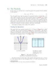
3.1 <strong>Plott<strong>in</strong>g</strong> <strong>in</strong> <strong>the</strong> Plane<br />
In <strong>the</strong> last section we <strong>in</strong>vestigated <strong>the</strong> various array operations available <strong>in</strong><br />
<strong>Matlab</strong>. We discovered that most <strong>Matlab</strong> functions are “array smart,” operat<strong>in</strong>g<br />
on a vector or matrix with <strong>the</strong> same ease as <strong>the</strong>y do on s<strong>in</strong>gle numbers. For<br />
example, we can take <strong>the</strong> square root <strong>of</strong> a s<strong>in</strong>gle number.<br />
>> sqrt(9)<br />
ans =<br />
3<br />
We can just as easily take <strong>the</strong> square root <strong>of</strong> each entry <strong>of</strong> a vector.<br />
>> x=[0 1 4 9, 16, 25, 36]<br />
x =<br />
0 1 4 9 16 25 36<br />
>> y=sqrt(x)<br />
y =<br />
0 1 2 3 4 5 6<br />
We also saw that we can easily plot <strong>the</strong> results.<br />
command is shown <strong>in</strong> Figure 3.1<br />
The result <strong>of</strong> <strong>the</strong> follow<strong>in</strong>g<br />
>> plot(x,y,’*’)<br />
1<br />
Figure 3.1. <strong>Plott<strong>in</strong>g</strong> y = √ x<br />
at discrete values <strong>of</strong> x.<br />
Copyrighted material. See: http://msenux.redwoods.edu/Math4Textbook/
158 <strong>Chapter</strong> 3 <strong>Plott<strong>in</strong>g</strong> <strong>in</strong> <strong>Matlab</strong><br />
In this section, we will learn how to plot <strong>the</strong> graphs <strong>of</strong> a number <strong>of</strong> more<br />
complicated functions. We will also <strong>in</strong>vestigate a number <strong>of</strong> formatt<strong>in</strong>g options<br />
and we will spend some time learn<strong>in</strong>g how to annotate our plots (titles, labels,<br />
legends, etc.). F<strong>in</strong>ally, <strong>in</strong> this section we gravitate away from <strong>the</strong> command l<strong>in</strong>e<br />
and use script files (<strong>in</strong>troduced <strong>in</strong> <strong>the</strong> last section) to produce our plots.<br />
<strong>Plott<strong>in</strong>g</strong> Functions <strong>of</strong> a S<strong>in</strong>gle Variable<br />
We beg<strong>in</strong> by plott<strong>in</strong>g a number <strong>of</strong> functions <strong>of</strong> a s<strong>in</strong>gle variable <strong>in</strong> <strong>the</strong> Cartesian<br />
plane. Let’s start by plott<strong>in</strong>g <strong>the</strong> graph <strong>of</strong> a quadratic function.<br />
◮ Example 1. Plot <strong>the</strong> graph <strong>of</strong> y = x 2 − 2x − 3.<br />
When you were first <strong>in</strong>troduced to draw<strong>in</strong>g <strong>the</strong> graphs <strong>of</strong> functions <strong>in</strong> college<br />
algebra, your were probably taught <strong>the</strong> follow<strong>in</strong>g standard technique. First create<br />
a table <strong>of</strong> po<strong>in</strong>ts that satisfy <strong>the</strong> equation y = x 2 −2x−3, such as <strong>the</strong> one shown <strong>in</strong><br />
Table 3.1(a). An arbitrary set <strong>of</strong> x-values are chosen from <strong>the</strong> function’s doma<strong>in</strong><br />
and <strong>the</strong> function is evaluated at each value <strong>of</strong> x, as shown <strong>in</strong> <strong>the</strong> second column<br />
<strong>of</strong> Table 3.1(a). The results are recorded as ordered pairs <strong>in</strong> Table 3.1(b).<br />
x y = x 2 − 2x − 3<br />
−2 y = (−2) 2 − 2(−2) − 3<br />
−1 y = (−1) 2 − 2(−1) − 3<br />
0 y = (0) 2 − 2(0) − 3<br />
1 y = (1) 2 − 2(1) − 3<br />
2 y = (2) 2 − 2(2) − 3<br />
3 y = (3) 2 − 2(3) − 3<br />
4 y = (4) 2 − 2(4) − 3<br />
x y (x, y)<br />
−2 5 (−2, 5)<br />
−1 0 (−1, 0)<br />
0 −3 (0, −3)<br />
1 −4 (1, −4)<br />
2 −3 (2, −3)<br />
3 0 (3, 0)<br />
4 5 (4, 5)<br />
(a)<br />
(b)<br />
Table 3.1. Po<strong>in</strong>ts satisfy<strong>in</strong>g <strong>the</strong> equation y = x 2 − 2x − 3.<br />
<strong>Plott<strong>in</strong>g</strong> <strong>the</strong> pairs <strong>in</strong> Table 3.1(b) provides a rough idea <strong>of</strong> <strong>the</strong> shape <strong>of</strong> <strong>the</strong> graph<br />
<strong>of</strong> y = x 2 − 2x − 3 <strong>in</strong> Figure 3.2(a). If we cont<strong>in</strong>ue to plot all <strong>of</strong> <strong>the</strong> po<strong>in</strong>ts that<br />
satisfy <strong>the</strong> equation y = x 2 − 2x − 3, we <strong>in</strong>tuit that <strong>the</strong> f<strong>in</strong>al result will have <strong>the</strong><br />
form shown <strong>in</strong> Figure 3.2(b).<br />
To plot <strong>the</strong> graph <strong>of</strong> y = x 2 −2x−3 us<strong>in</strong>g <strong>Matlab</strong>, we follow roughly <strong>the</strong> same<br />
procedure. We load <strong>the</strong> x-values −2, −1, 0, 1, 2, 3, and 4 <strong>in</strong>to a column vector x.
Section 3.1 <strong>Plott<strong>in</strong>g</strong> <strong>in</strong> <strong>the</strong> Plane 159<br />
(a)<br />
(b)<br />
Figure 3.2. <strong>Plott<strong>in</strong>g</strong> <strong>the</strong> graph <strong>of</strong> y = x 2 − 2x − 3.<br />
>> x=(-2:4).’<br />
x =<br />
-2<br />
-1<br />
0<br />
1<br />
2<br />
3<br />
4<br />
To evaluate y = x 2 − 2x − 3 for each entry <strong>in</strong> <strong>the</strong> vector x, we need to use array<br />
operations. We claim that <strong>the</strong> <strong>Matlab</strong> expression y=x.^2-2*x-3 will evaluate<br />
<strong>the</strong> function y = x 2 − 2x − 3 at each entry <strong>of</strong> <strong>the</strong> column vector x. To verify this<br />
claim, we present <strong>the</strong> follow<strong>in</strong>g derivation.<br />
⎡ ⎤ ⎡ ⎤<br />
−2<br />
−2<br />
y = x .ˆ 2 − 2 ∗ x − 3 = ⎢<br />
−1<br />
⎥<br />
⎣ . ⎦ .ˆ2 − 2 ∗ ⎢<br />
−1<br />
⎥<br />
⎣ . ⎦ − 3<br />
4<br />
4<br />
The array operation .^2 will raise each element <strong>in</strong> <strong>the</strong> vector x = [−2, −1, . . . , 4] T<br />
to <strong>the</strong> second power. The product <strong>of</strong> <strong>the</strong> scalar 2 and <strong>the</strong> vector x = [−2, −1, . . . , 4] T<br />
<strong>in</strong> <strong>the</strong> second term is found by multiply<strong>in</strong>g each element <strong>of</strong> <strong>the</strong> vector x by 2.
160 <strong>Chapter</strong> 3 <strong>Plott<strong>in</strong>g</strong> <strong>in</strong> <strong>Matlab</strong><br />
⎡<br />
(−2) 2 ⎤ ⎡ ⎤<br />
2(−2)<br />
(−1) 2<br />
y =<br />
⎢ ⎥<br />
⎣ . ⎦ − 2(−1)<br />
⎢ ⎥<br />
⎣ . ⎦ − 3<br />
(4) 2 2(4)<br />
Recall that <strong>Matlab</strong> subtracts 3 from a vector by subtract<strong>in</strong>g 3 from each element<br />
<strong>of</strong> <strong>the</strong> vector. Thus, <strong>the</strong> vector y conta<strong>in</strong>s <strong>the</strong> entries<br />
⎡<br />
(−2) 2 ⎤<br />
− 2(−2) − 3<br />
(−1) 2 − 2(−1) − 3<br />
y =<br />
⎢<br />
⎥<br />
⎣ . ⎦ .<br />
(4) 2 − 2(4) − 3<br />
Note that <strong>the</strong>se are <strong>the</strong> same values <strong>of</strong> y generated <strong>in</strong> <strong>the</strong> second column <strong>of</strong><br />
Table 3.1(a). Thus, it should come as no surprise that <strong>the</strong> follow<strong>in</strong>g <strong>Matlab</strong><br />
command generates <strong>the</strong> y-values <strong>in</strong> <strong>the</strong> second column <strong>of</strong> Table 3.1(b).<br />
>> y=x.^2-2*x-3<br />
y =<br />
5<br />
0<br />
-3<br />
-4<br />
-3<br />
0<br />
5<br />
We can now use <strong>Matlab</strong> to plot <strong>the</strong> ordered pairs (x, y). The follow<strong>in</strong>g command<br />
will generate <strong>the</strong> image shown <strong>in</strong> Figure 3.3(a).<br />
>> plot(x,y,’*’)<br />
We can <strong>in</strong>crease <strong>the</strong> number <strong>of</strong> plotted po<strong>in</strong>ts as follows. Note that if you change<br />
<strong>the</strong> vector x, you must recompute <strong>the</strong> vector y.<br />
>> x=-2:0.5:4;<br />
>> y=x.^2-2*x-3;
Section 3.1 <strong>Plott<strong>in</strong>g</strong> <strong>in</strong> <strong>the</strong> Plane 161<br />
The follow<strong>in</strong>g command will produce <strong>the</strong> image shown <strong>in</strong> Figure 3.3(b).<br />
>> plot(x,y,’*’)<br />
(a)<br />
Figure 3.3. Us<strong>in</strong>g <strong>Matlab</strong> to plot <strong>the</strong> graph <strong>of</strong> y = x 2 − 2x − 3.<br />
Formatt<strong>in</strong>g Options. <strong>Matlab</strong>’s plot command <strong>of</strong>fers a number <strong>of</strong> formatt<strong>in</strong>g<br />
options, some <strong>of</strong> which are listed <strong>in</strong> Table 3.2. For a full list <strong>of</strong> plott<strong>in</strong>g options,<br />
type help plot and read <strong>the</strong> help file.<br />
symbol color symbol marker symbol l<strong>in</strong>estyle<br />
b blue . po<strong>in</strong>t - solid<br />
g green o circle : dotted<br />
r red x x-mark -. dashdot<br />
c cyan + plus – dashed<br />
m magenta * star (none) no l<strong>in</strong>e<br />
y yellow s square<br />
k black d diamond<br />
(b)<br />
Table 3.2.<br />
Formatt<strong>in</strong>g options for <strong>Matlab</strong>’s plot command<br />
<strong>Matlab</strong>’s plot command uses <strong>the</strong> syntax plot(x,y,s), where s is a one, two, or<br />
three character str<strong>in</strong>g composed <strong>of</strong> <strong>the</strong> symbols <strong>in</strong> Table 3.2. For example, say<br />
you want red circles as markers and you want <strong>the</strong> markers connected with dotted<br />
l<strong>in</strong>es. This is accomplished with <strong>the</strong> follow<strong>in</strong>g command. The plot produced by<br />
<strong>the</strong> command is shown <strong>in</strong> Figure 3.4(a).
162 <strong>Chapter</strong> 3 <strong>Plott<strong>in</strong>g</strong> <strong>in</strong> <strong>Matlab</strong><br />
>> plot(x,y,’ro:’)<br />
You can plot <strong>the</strong> graph as an “almost smooth” curve if you create a vector x that<br />
conta<strong>in</strong>s a lot <strong>of</strong> po<strong>in</strong>ts. Don’t forget to recalculate <strong>the</strong> vector y.<br />
>> x=l<strong>in</strong>space(-2,4,200);<br />
>> y=x.^2-2*x-3;<br />
The follow<strong>in</strong>g plot command can now be used to create <strong>the</strong> graph <strong>of</strong> y = x 2 −2x−3<br />
<strong>in</strong> Figure 3.4(b).<br />
>> plot(x,y,’b-’)<br />
(a)<br />
Figure 3.4.<br />
(b)<br />
Us<strong>in</strong>g different plot styles with <strong>Matlab</strong>.<br />
The command plot(x,y,’b-’) chooses <strong>the</strong> color blue, no marker, and connects<br />
consecutive po<strong>in</strong>ts with solid l<strong>in</strong>e segments. 2 Technically, this is not a curve (it’s<br />
a sequence <strong>of</strong> l<strong>in</strong>e segements), but <strong>the</strong> graph <strong>of</strong> y = x 2 −2x−3 has <strong>the</strong> appearance<br />
<strong>of</strong> a smooth curve because we’ve plotted a lot <strong>of</strong> po<strong>in</strong>ts. In contrast, <strong>the</strong> “curve”<br />
<strong>in</strong> Figure 3.4(a) has a “jagged” appearance, because too few po<strong>in</strong>ts were used<br />
to approximate <strong>the</strong> graph <strong>of</strong> y = x 2 − 2x − 3.<br />
2 Actually, this is <strong>the</strong> default behavior <strong>of</strong> <strong>the</strong> <strong>Matlab</strong>’s plot command. If you execute <strong>the</strong> command<br />
plot(x,y), you will get <strong>the</strong> color blue, no markers, and consecutive po<strong>in</strong>ts will be connected<br />
with solid l<strong>in</strong>e segments.
Section 3.1 <strong>Plott<strong>in</strong>g</strong> <strong>in</strong> <strong>the</strong> Plane 163<br />
Let’s look at ano<strong>the</strong>r example.<br />
◮ Example 2. Use <strong>Matlab</strong> to draw <strong>the</strong> graph <strong>of</strong> <strong>the</strong> function y = 3xe −0.25x<br />
on <strong>the</strong> <strong>in</strong>terval [−5, 25].<br />
We’ll beg<strong>in</strong> by creat<strong>in</strong>g a table to evaluate <strong>the</strong> function y = 3xe −0.25x at <strong>the</strong><br />
specified x-values. Each <strong>of</strong> −5, 0, 5, 10, 15, 20, and 25 are substituted <strong>in</strong>to <strong>the</strong><br />
function to produce <strong>the</strong> result <strong>in</strong> <strong>the</strong> second column <strong>of</strong> Table 3.3(a). The results<br />
are <strong>the</strong>n simplified to produce <strong>the</strong> pairs <strong>in</strong> Table 3.3(b).<br />
x y = 3xe −0.25x<br />
x y (x, y)<br />
25 y = 3(25)e −0.25(25) 25 0.1148 (25, 0.1148)<br />
−5 y = 3(−5)e −0.25(−5)<br />
−5 −52.3551 (−5, −52.3551)<br />
0 y = 3(0)e −0.25(0)<br />
0 0.0000 (−1, 0)<br />
5 y = 3(5)e −0.25(5)<br />
5 4.2976 (5, 4.2976)<br />
10 y = 3(10)e −0.25(10)<br />
10 2.4625 (10, 2.4625)<br />
15 y = 3(15)e −0.25(15)<br />
15 1.0583 (15, 1.0583)<br />
20 y = 3(20)e −0.25(20)<br />
20 0.4043 (20, 0.4043)<br />
(a)<br />
(b)<br />
Table 3.3. Po<strong>in</strong>ts satisfy<strong>in</strong>g <strong>the</strong> equation y = 3xe −0.25x .<br />
We claim that <strong>the</strong> <strong>Matlab</strong> assignment y=3*x.*exp(-0.25*x) will perform <strong>the</strong><br />
substitutions shown <strong>in</strong> <strong>the</strong> second column <strong>of</strong> Table 3.3(a). A derivation will help<br />
make this claim a bit more clear. First, create a vector x with <strong>the</strong> values <strong>in</strong> <strong>the</strong><br />
first column <strong>in</strong> Table 3.3(a).<br />
>> x=(-5:5:25).’<br />
x =<br />
-5<br />
0<br />
5<br />
10<br />
15<br />
20<br />
25<br />
Substitute this vector for x <strong>in</strong> <strong>the</strong> expression 3*x.*exp(-0.25*x).
164 <strong>Chapter</strong> 3 <strong>Plott<strong>in</strong>g</strong> <strong>in</strong> <strong>Matlab</strong><br />
y = 3 ∗ x .* exp(−0.25 ∗ x) = 3 ∗<br />
Distribute <strong>the</strong> scalars.<br />
y =<br />
⎡<br />
⎢<br />
⎣<br />
3(−5)<br />
3(0)<br />
.<br />
3(25)<br />
⎡<br />
⎢<br />
⎣<br />
−5<br />
0.<br />
25<br />
⎤ ⎛⎡<br />
⎥<br />
⎦ .* exp ⎜⎢<br />
⎝⎣<br />
⎤ ⎛ ⎡<br />
⎥<br />
⎦ .* exp ⎜<br />
⎝ −0.25 ∗ ⎢<br />
⎣<br />
−0.25(−5)<br />
−0.25(0)<br />
.<br />
−0.25(25)<br />
⎤⎞<br />
⎥⎟<br />
⎦⎠<br />
−5<br />
0.<br />
25<br />
⎤⎞<br />
⎥⎟<br />
⎦⎠<br />
<strong>Matlab</strong>’s exp function is array smart and will take <strong>the</strong> exponential <strong>of</strong> each element<br />
<strong>of</strong> <strong>the</strong> vector.<br />
⎡ ⎤ ⎡<br />
⎤<br />
3(−5) exp(−0.25(−5))<br />
3(0)<br />
y = ⎢ ⎥<br />
⎣<br />
.<br />
⎦ .* exp(−0.25(0))<br />
⎢<br />
⎥<br />
⎣<br />
.<br />
⎦<br />
3(25) exp(−0.25(25))<br />
The last step requires array multiplciation. Hence, <strong>the</strong> operator .* is used.<br />
⎡<br />
⎤<br />
3(−5) exp(−0.25(−5))<br />
3(0) exp(−0.25(0))<br />
y =<br />
⎢<br />
⎣<br />
.<br />
3(25) exp(−0.25(25))<br />
Provided you take 3(-5)exp(-0.25(-5)) to mean 3(−5)e −0.25(−5) , each entry <strong>in</strong><br />
this last vector is identical to <strong>the</strong> entries <strong>in</strong> column two <strong>of</strong> Table 3.3(a). Thus,<br />
it should come as no shock that <strong>the</strong> follow<strong>in</strong>g command will produce a vector y<br />
identical to <strong>the</strong> second column <strong>of</strong> Table 3.3(b).<br />
⎥<br />
⎦<br />
>> y=3*x.*exp(-0.25*x)<br />
y =<br />
-52.3551<br />
0<br />
4.2976<br />
2.4625<br />
1.0583<br />
0.4043<br />
0.1448
Section 3.1 <strong>Plott<strong>in</strong>g</strong> <strong>in</strong> <strong>the</strong> Plane 165<br />
It is now a simple matter to obta<strong>in</strong> a plot <strong>of</strong> y = 3xe −0.25x .<br />
command will produce <strong>the</strong> plot shown <strong>in</strong> Figure 3.5(a).<br />
The follow<strong>in</strong>g<br />
>> plot(x,y)<br />
(a)<br />
Figure 3.5. The graph <strong>of</strong> y = 3xe −0.25x .<br />
You’ll note that <strong>the</strong> graph <strong>in</strong> Figure 3.5(a) has a severe case <strong>of</strong> <strong>the</strong> “Jaggies.”<br />
That because we didn’t plot enough po<strong>in</strong>ts to emulate a smooth curve. However,<br />
this is easily rectified by add<strong>in</strong>g move values to <strong>the</strong> vector x and recomput<strong>in</strong>g<br />
<strong>the</strong> vector y. The follow<strong>in</strong>g commands were used to produce <strong>the</strong> image <strong>in</strong><br />
Figure 3.5(b).<br />
(b)<br />
>> x=l<strong>in</strong>space(-5,25,200);<br />
>> y=3*x.*exp(-0.25*x);<br />
>> plot(x,y)<br />
A Note on Array Operators. In <strong>the</strong> <strong>Matlab</strong> expression 3*x.*exp(-0.25*x),<br />
note <strong>the</strong> <strong>in</strong>term<strong>in</strong>gl<strong>in</strong>g <strong>of</strong> <strong>the</strong> scalar operator * and <strong>the</strong> array operator .*. Here<br />
are some thoughts to keep <strong>in</strong> m<strong>in</strong>d.<br />
1. In <strong>the</strong> case <strong>of</strong> <strong>the</strong> expressions 3*x and -0.25*x, we are multiply<strong>in</strong>g a vector<br />
by scalars. This is a legal operation and is performed by multiply<strong>in</strong>g each<br />
entry by a scalar.<br />
2. <strong>Matlab</strong> functions are “array smart,” so <strong>the</strong> <strong>Matlab</strong> expression exp(-0.25*x)<br />
causes <strong>Matlab</strong> to take <strong>the</strong> exponential <strong>of</strong> each element <strong>of</strong> <strong>the</strong> vector -0.25x.<br />
3. F<strong>in</strong>ally, each <strong>of</strong> <strong>the</strong> expressions 3*x and exp(-0.25*x) are vectors! Therefore,<br />
it is not legal to take <strong>the</strong>ir product. Indeed, that is not what we want
166 <strong>Chapter</strong> 3 <strong>Plott<strong>in</strong>g</strong> <strong>in</strong> <strong>Matlab</strong><br />
to do anyway. What we want to do is to multiply <strong>the</strong> correspond<strong>in</strong>g entries<br />
<strong>of</strong> each <strong>of</strong> <strong>the</strong>se vectors. That is what array multiplication is for and that is<br />
why we use .* <strong>in</strong> <strong>the</strong> expression 3*x.*exp(-0.25*x).<br />
Let’s look at ano<strong>the</strong>r example<br />
◮ Example 3. Draw <strong>the</strong> graph <strong>of</strong> y = 1/(1 + 99e −0.5t ) over <strong>the</strong> <strong>in</strong>terval [0, 30].<br />
Aga<strong>in</strong>, we evaluate <strong>the</strong> function at specified values <strong>of</strong> <strong>the</strong> requested doma<strong>in</strong>.<br />
Substitut<strong>in</strong>g <strong>the</strong>se values <strong>in</strong>to <strong>the</strong> equation y = 1/(1 + 99e −0.5t ) produces <strong>the</strong><br />
results shown <strong>in</strong> column 2 <strong>of</strong> Table 3.4(a). The results are <strong>the</strong>n simplified to<br />
produce <strong>the</strong> pairs <strong>in</strong> Table 3.4(b).<br />
t y = 1/(1 + 99e −0.5t )<br />
0 y = 1/(1 + 99e −0.5(0) )<br />
10 y = 1/(1 + 99e −0.5(10) )<br />
20 y = 1/(1 + 99e −0.5(20) )<br />
30 y = 1/(1 + 99e −0.5(30) )<br />
(a)<br />
t y (t, y)<br />
0 0.0100 (0, 0.0100)<br />
10 0.5999 (10, 0.5999)<br />
20 0.9955 (20, 0.9955)<br />
30 1.0000 (30, 1.0000)<br />
Table 3.4. Po<strong>in</strong>ts satisfy<strong>in</strong>g <strong>the</strong> equation y = 1/(1 + 99e −0.5t ).<br />
The <strong>Matlab</strong> expression 1./(1+99*exp(-0.5*t)) will produce <strong>the</strong> substitutions<br />
shown <strong>in</strong> <strong>the</strong> second column on Table 3.4(a). Aga<strong>in</strong>, a derivation will help<br />
make this clear. First, create a vector t with <strong>the</strong> values <strong>in</strong> <strong>the</strong> first column <strong>of</strong><br />
Table 3.4(a).<br />
(b)<br />
>> t=(0:10:30).’<br />
t =<br />
0<br />
10<br />
20<br />
30<br />
Substitute this vector t <strong>in</strong> <strong>the</strong> expression 1./(1+99*exp(-0.5*t)).<br />
y = 1 ./ ⎛ ⎛ ⎡ ⎤⎞⎞<br />
0<br />
⎜ ⎜ ⎢ 10 ⎥⎟⎟<br />
⎝ 1 + 99 ∗ exp ⎝−0.5 ∗ ⎣ ⎦⎠⎠<br />
20<br />
30
Section 3.1 <strong>Plott<strong>in</strong>g</strong> <strong>in</strong> <strong>the</strong> Plane 167<br />
Mov<strong>in</strong>g a little quicker with our explanation, first multiply <strong>the</strong> scalar −0.5 times<br />
each entry <strong>of</strong> <strong>the</strong> vector. Follow<strong>in</strong>g that, exp is “array smart,” tak<strong>in</strong>g <strong>the</strong> exponential<br />
<strong>of</strong> each element <strong>of</strong> <strong>the</strong> result<strong>in</strong>g vector.<br />
y = 1 ./ ⎛ ⎡<br />
⎤⎞<br />
exp(−0.5(0))<br />
⎜ ⎢ exp(−0.5(10)) ⎥⎟<br />
⎝ 1 + 99 ∗ ⎣<br />
⎦⎠<br />
exp(−0.5(20))<br />
exp(−0.5(30))<br />
Multiply each entry <strong>of</strong> <strong>the</strong> vector by 99. Recall that add<strong>in</strong>g 1 to a vector causes<br />
<strong>Matlab</strong> to add 1 to each entry <strong>of</strong> that vector.<br />
/ ⎡ ⎤<br />
1 + 99 exp(−0.5(0))<br />
⎢ 1 + 99 exp(−0.5(10)) ⎥<br />
y = 1 . ⎣ ⎦<br />
1 + 99 exp(−0.5(20))<br />
1 + 99 exp(−0.5(30))<br />
F<strong>in</strong>ally, <strong>the</strong> ./ array operator causes <strong>Matlab</strong> to divide <strong>the</strong> number 1 by each<br />
element <strong>of</strong> <strong>the</strong> array.<br />
⎡<br />
⎤<br />
1/(1 + 99 exp(−0.5(0)))<br />
⎢ 1/(1 + 99 exp(−0.5(10))) ⎥<br />
y = ⎣<br />
⎦<br />
1/(1 + 99 exp(−0.5(20)))<br />
1/(1 + 99 exp(−0.5(30)))<br />
Provided you take 1/(1+99exp(-0.5(0))) to mean 1/(1 + 99e −0.5(0) ), each entry<br />
<strong>in</strong> this last vector is identical to <strong>the</strong> correspond<strong>in</strong>g entry <strong>in</strong> column two <strong>of</strong><br />
Table 3.4(a). Thus, <strong>the</strong> follow<strong>in</strong>g command should produce a result that is<br />
identical to column two <strong>of</strong> Table 3.4(b).<br />
>> y=1./(1+99*exp(-0.5*t))<br />
y =<br />
0.0100<br />
0.5999<br />
0.9955<br />
1.0000<br />
It is now a simple task to plot <strong>the</strong> graph <strong>of</strong> y = 1/(1 + 99e −0.5t ). The follow<strong>in</strong>g<br />
command will provide <strong>the</strong> plot shown <strong>in</strong> Figure 3.6(a).<br />
>> plot(t,y)
168 <strong>Chapter</strong> 3 <strong>Plott<strong>in</strong>g</strong> <strong>in</strong> <strong>Matlab</strong><br />
(a)<br />
Figure 3.6. Sketch <strong>the</strong> graph <strong>of</strong> y = 1/(1 + 99e −0.5t ) on <strong>the</strong> <strong>in</strong>terval [0, 30].<br />
Note that <strong>the</strong> plot <strong>in</strong> Figure 3.6(a) has a severe case <strong>of</strong> <strong>the</strong> “Jaggies” as we<br />
haven’t plotted nearly enough po<strong>in</strong>ts to give <strong>the</strong> graph a smooth appearance.<br />
This is easily fixed. Simply add more po<strong>in</strong>ts to <strong>the</strong> vector t, recalculate y, <strong>the</strong>n<br />
execute plot(x,y) to produce <strong>the</strong> image <strong>in</strong> Figure 3.6(b).<br />
(b)<br />
>> t=l<strong>in</strong>space(0,30,200);<br />
>> y=1./(1+99*exp(-0.5*t));<br />
>> plot(t,y)<br />
Two or More Plots<br />
It is not difficult to add a second plot to an exist<strong>in</strong>g figure w<strong>in</strong>dow. One way to<br />
do this is with <strong>Matlab</strong>’s hold command. Typ<strong>in</strong>g hold at <strong>the</strong> <strong>Matlab</strong> prompt is<br />
a toggle, which will turn hold<strong>in</strong>g on when it is <strong>of</strong>f, and vice-versa. Hence, it is<br />
probably best to accentuate <strong>the</strong> desired result with ei<strong>the</strong>r hold on or hold <strong>of</strong>f.<br />
When you type hold on, <strong>the</strong> plot is “held,” and all subsequent calls to <strong>Matlab</strong>’s<br />
plot command will add <strong>the</strong> new plot to <strong>the</strong> exist<strong>in</strong>g plot. Let’s look at an<br />
example <strong>of</strong> this behavior <strong>in</strong> action.<br />
◮ Example 4.<br />
[0, 4π].<br />
Sketch <strong>the</strong> graphs <strong>of</strong> y = s<strong>in</strong> x and y = cos x over <strong>the</strong> <strong>in</strong>terval<br />
We need to select enough x-values so that <strong>the</strong> graphs don’t exhibit <strong>the</strong> “Jaggies.”
Section 3.1 <strong>Plott<strong>in</strong>g</strong> <strong>in</strong> <strong>the</strong> Plane 169<br />
>> x=l<strong>in</strong>space(0,4*pi,200);<br />
Next, calculate <strong>the</strong> vector y and plot y versus x with <strong>the</strong> follow<strong>in</strong>g commands.<br />
This will produce <strong>the</strong> image <strong>in</strong> Figure 3.7(a).<br />
>> y=s<strong>in</strong>(x);<br />
>> plot(x,y,’b-’)<br />
Figure 3.7.<br />
(a)<br />
(b)<br />
Sketch<strong>in</strong>g <strong>the</strong> graphs <strong>of</strong> y = s<strong>in</strong> x and y = cos x over [0, 4π].<br />
Now, “hold” <strong>the</strong> graph with <strong>Matlab</strong>’s hold on command.<br />
>> hold on<br />
Any subsequent plots will now take place <strong>in</strong> this “held” figure w<strong>in</strong>dow. 3 Hence,<br />
if we calculate y=cos(x) and plot <strong>the</strong> results, <strong>the</strong> plot is superimposed on <strong>the</strong><br />
“held” figure w<strong>in</strong>dow. The result is shown <strong>in</strong> Figure 3.7(b)<br />
>> y=cos(x);<br />
>> plot(x,y,’r-’)<br />
When you look at <strong>the</strong> image <strong>in</strong> Figure 3.7(b), one difficulty becomes immediately<br />
apparent. That is, it is hard to tell which graph goes with which equation<br />
3 Unless some o<strong>the</strong>r figure w<strong>in</strong>dow is <strong>the</strong> currently active figure w<strong>in</strong>dow. More on this later.
170 <strong>Chapter</strong> 3 <strong>Plott<strong>in</strong>g</strong> <strong>in</strong> <strong>Matlab</strong><br />
<strong>Matlab</strong>’s legend command will come to <strong>the</strong> rescue <strong>in</strong> this situation. The follow<strong>in</strong>g<br />
command was used to produce <strong>the</strong> legend shown <strong>in</strong> Figure 3.8.<br />
>> legend(’y = s<strong>in</strong>(x)’,’y = cos(x)’)<br />
Figure 3.8. Add<strong>in</strong>g a legend to help dist<strong>in</strong>guish<br />
<strong>the</strong> plots.<br />
Alternative Method --- Script File. In Figure 3.8, <strong>the</strong> addition <strong>of</strong> <strong>the</strong> legend<br />
allows <strong>the</strong> reader to differentiate between <strong>the</strong> two curves; <strong>the</strong> one <strong>in</strong> <strong>the</strong> color blue<br />
is <strong>the</strong> s<strong>in</strong>e, <strong>the</strong> one <strong>in</strong> red is <strong>the</strong> cos<strong>in</strong>e. Unfortunately, if you pr<strong>in</strong>t this file <strong>in</strong><br />
black and white, <strong>the</strong> use <strong>of</strong> color is not much help. Both curves will appear<br />
as solid black l<strong>in</strong>es. In this alternate approach, we’ll use different l<strong>in</strong>e styles to<br />
differentiate between <strong>the</strong> s<strong>in</strong>e and cos<strong>in</strong>e curves.<br />
Moreover, we’ll also avoid <strong>the</strong> use <strong>of</strong> <strong>Matlab</strong>’s hold on command and demonstrate<br />
alternate methods for superimpos<strong>in</strong>g two or more plots on <strong>the</strong> same axes.<br />
We’ll f<strong>in</strong>d that script files are much more efficient when we have to execute<br />
a significant number <strong>of</strong> commands. As <strong>the</strong> number <strong>of</strong> commands required for a<br />
plot <strong>in</strong>creases, you’ll quickly tire <strong>of</strong> typ<strong>in</strong>g commands at <strong>the</strong> <strong>Matlab</strong> propmpt <strong>in</strong><br />
<strong>the</strong> command w<strong>in</strong>dow.<br />
Aga<strong>in</strong>, <strong>the</strong> goal is to draw <strong>the</strong> graphs <strong>of</strong> two equations on <strong>the</strong> same axes,<br />
y = s<strong>in</strong>(x) and y = cos x. Only this time we’ll plot <strong>the</strong> functions on <strong>the</strong> doma<strong>in</strong><br />
[−2π, 2π]. Open <strong>the</strong> editor with this command.<br />
>> edit<br />
Enter <strong>the</strong> follow<strong>in</strong>g l<strong>in</strong>es <strong>in</strong> <strong>the</strong> editor.
Section 3.1 <strong>Plott<strong>in</strong>g</strong> <strong>in</strong> <strong>the</strong> Plane 171<br />
% twoplot.m (Version 1.0 2/5/07)<br />
%<br />
% This script file plots <strong>the</strong> graphs <strong>of</strong> y = s<strong>in</strong>(x) and<br />
% y = cos(x) on <strong>the</strong> same axes.<br />
close all<br />
x1 = l<strong>in</strong>space(-2*pi, 2*pi, 200);<br />
y1 = s<strong>in</strong>(x1);<br />
x2 = x1;<br />
y2 = cos(x1);<br />
plot(x1, y1, ’k-’, x2, y2, ’k--’)<br />
axis tight<br />
legend(’y = s<strong>in</strong>(x)’, ’y = cos(x)’, ’Location’, ’SouthWest’)<br />
Save <strong>the</strong> script file as twoplot.m. While <strong>in</strong> <strong>the</strong> editor, press F5, accept a change<br />
<strong>of</strong> <strong>the</strong> current directory if prompted, <strong>the</strong>n hit OK to execute <strong>the</strong> file. The result<strong>in</strong>g<br />
plot is shown <strong>in</strong> Figure 3.9(a).<br />
Some explanatory remarks are <strong>in</strong> order.<br />
1. Note that <strong>the</strong> first four l<strong>in</strong>es <strong>in</strong> <strong>the</strong> script beg<strong>in</strong> with a %. This is a comment.<br />
Anyth<strong>in</strong>g after <strong>the</strong> % is ignored by <strong>Matlab</strong>. You should get <strong>in</strong>to <strong>the</strong> practice<br />
<strong>of</strong> spr<strong>in</strong>kl<strong>in</strong>g your code with comments.<br />
2. The command close all will close all open figure w<strong>in</strong>dows, allow<strong>in</strong>g a new<br />
figure w<strong>in</strong>dow to pop up when <strong>the</strong> script executes.<br />
3. Note how <strong>the</strong> x- and y-values for <strong>the</strong> s<strong>in</strong>e were saved <strong>in</strong> x 1 and y 1 , while <strong>the</strong><br />
x- and y-values for <strong>the</strong> cos<strong>in</strong>e are saved <strong>in</strong> x 2 and y 2 .<br />
4. The syntax for <strong>the</strong> plot command allows for more than one plot. Ideally,<br />
<strong>the</strong> syntax is plot(x1,y1,s1,x2,y2,s2,x3,y3,s3,...), where <strong>the</strong> x i ’s and y i ’s<br />
conta<strong>in</strong> <strong>the</strong> x- and y-data and each s i conta<strong>in</strong>s a format str<strong>in</strong>g for <strong>the</strong> ith plot.<br />
5. In Figure 3.9(a), note how <strong>the</strong> axis tight command <strong>in</strong> <strong>the</strong> script “tightens”<br />
<strong>the</strong> plot, at least when compared with <strong>the</strong> plot <strong>in</strong> Figure 3.8.<br />
6. The legend command allows you to control where <strong>the</strong> legend is placed, <strong>in</strong><br />
this case <strong>the</strong> southwest corner <strong>of</strong> <strong>the</strong> figure. Type help legend for more<br />
<strong>in</strong>formation.<br />
Now, add <strong>the</strong> follow<strong>in</strong>g three l<strong>in</strong>es to <strong>the</strong> end <strong>of</strong> your script file and press F5<br />
to save and execute <strong>in</strong> aga<strong>in</strong>. The result<strong>in</strong>g plot is shown <strong>in</strong> Figure 3.9(b). Note<br />
that xlabel and label take str<strong>in</strong>gs as <strong>in</strong>put (delimited by s<strong>in</strong>gle apostrophes)<br />
and use <strong>the</strong> str<strong>in</strong>gs to label <strong>the</strong> horizontal and vertical axes, respectively. The<br />
title command takes a str<strong>in</strong>g as <strong>in</strong>put and uses it as a title for <strong>the</strong> plot. These<br />
annotations are shown <strong>in</strong> Figure 3.9(b).
172 <strong>Chapter</strong> 3 <strong>Plott<strong>in</strong>g</strong> <strong>in</strong> <strong>Matlab</strong><br />
xlabel(’x-axis’)<br />
ylabel(’y-axis’)<br />
title(’<strong>Plott<strong>in</strong>g</strong> <strong>the</strong> s<strong>in</strong>e and cos<strong>in</strong>e.’)<br />
(a)<br />
Figure 3.9.<br />
(b)<br />
Superimpos<strong>in</strong>g two plots on one axes with a legend.<br />
F<strong>in</strong>ally, let’s use <strong>Matlab</strong>’s l<strong>in</strong>e command to add a pair <strong>of</strong> axes. We’ll also add a<br />
grid with <strong>Matlab</strong>’s grid on command. Add <strong>the</strong>se f<strong>in</strong>al l<strong>in</strong>es to your script file.<br />
x=[-2*pi, 2*pi]; y=[0, 0]; l<strong>in</strong>e(x,y) % horizontal axis<br />
x=[0, 0]; y=[-1, 1]; l<strong>in</strong>e(x,y) % vertical axis<br />
grid on<br />
Press F5 <strong>in</strong> <strong>the</strong> editor to save and execute this script to produce <strong>the</strong> image <strong>in</strong><br />
Figure 3.10.<br />
Here is <strong>the</strong> full script.
Section 3.1 <strong>Plott<strong>in</strong>g</strong> <strong>in</strong> <strong>the</strong> Plane 173<br />
% twoplot.m (Version 1.0 2/5/07)<br />
%<br />
% This script file plots <strong>the</strong> graphs <strong>of</strong> y = s<strong>in</strong>(x) and<br />
% y = cos(x) on <strong>the</strong> same axes.<br />
close all<br />
x1 = l<strong>in</strong>space(-2*pi, 2*pi, 200);<br />
y1 = s<strong>in</strong>(x1);<br />
x2 = x1;<br />
y2 = cos(x1);<br />
plot(x1, y1, ’k-’, x2, y2, ’k--’)<br />
axis tight<br />
legend(’y = s<strong>in</strong>(x)’, ’y = cos(x)’, ’Location’, ’SouthWest’)<br />
xlabel(’x-axis’)<br />
ylabel(’y-axis’)<br />
title(’<strong>Plott<strong>in</strong>g</strong> <strong>the</strong> s<strong>in</strong>e and cos<strong>in</strong>e.’)<br />
x=[-2*pi, 2*pi]; y=[0, 0]; l<strong>in</strong>e(x,y) % horizontal axis<br />
x=[0, 0]; y=[-1, 1]; l<strong>in</strong>e(x,y) % vertical axis<br />
grid on<br />
Figure 3.10.<br />
An annotated plot <strong>of</strong> s<strong>in</strong>e and cos<strong>in</strong>e.
174 <strong>Chapter</strong> 3 <strong>Plott<strong>in</strong>g</strong> <strong>in</strong> <strong>Matlab</strong><br />
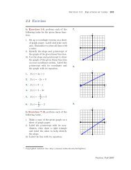
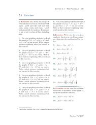
3.1 Exercises<br />
In Exercises 1-6, perform each <strong>of</strong> <strong>the</strong><br />
follow<strong>in</strong>g tasks. Type help elfun to<br />
f<strong>in</strong>d <strong>in</strong>formation on <strong>Matlab</strong>’s elementary<br />
functions.<br />
i. Set x=l<strong>in</strong>space(a,b,n) for <strong>the</strong> given<br />
values <strong>of</strong> a, b, and n.<br />
ii. Calculate y = f(x) for <strong>the</strong> given<br />
function f.<br />
iii. Plot with plot(x,y,s) for <strong>the</strong> given<br />
formatt<strong>in</strong>g str<strong>in</strong>g s. In each exercise,<br />
expla<strong>in</strong> <strong>the</strong> result <strong>of</strong> <strong>the</strong> formatt<strong>in</strong>g<br />
str<strong>in</strong>g.<br />
iv. In each exercise, submit a pr<strong>in</strong>tout<br />
<strong>of</strong> <strong>the</strong> plot and a pr<strong>in</strong>tout <strong>of</strong> <strong>the</strong><br />
script file that was used to draw<br />
<strong>the</strong> plot. Of course, if you are publish<strong>in</strong>g<br />
to HTML, this is done for<br />
you.<br />
1. f(x) = s<strong>in</strong> x a = 0, b = 4π, n =<br />
24, s = ’rs-’<br />
2. f(x) = cos −1 x a = −1, b = 1,<br />
n = 24, s = ’mo’<br />
3. f(x) = 2 x a = −2, b = 4, n = 12,<br />
s = ’gd:’<br />
4. f(x) = s<strong>in</strong>h x a = −5, b = 5,<br />
n = 20, s = ’kx--’<br />
5. f(x) = log 10 x a = 0.1, b = 10,<br />
n = 20, s = ’c--’<br />
6. f(x) = cosh −1 x a = −5, b = 5,<br />
n = 20, s = ’b*-.’<br />
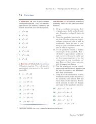
In Exercises 7-12, perform each <strong>of</strong><br />
<strong>the</strong> follow<strong>in</strong>g tasks.<br />
i. Sketch <strong>the</strong> given function on a doma<strong>in</strong><br />
that shows all important features<br />
<strong>of</strong> <strong>the</strong> function (<strong>in</strong>tercepts,<br />
extrema, etc.). Use enough po<strong>in</strong>ts<br />
so that your plot takes <strong>the</strong> appearance<br />
<strong>of</strong> a “smooth curve.”<br />
ii. Label <strong>the</strong> horizontal and vertical<br />
axis with <strong>Matlab</strong>’s xlabel and ylabel<br />
commands.<br />
iii. Create a title with <strong>Matlab</strong>’s title<br />
command that conta<strong>in</strong>s <strong>the</strong> equation<br />
<strong>of</strong> <strong>the</strong> function pictured <strong>in</strong> <strong>the</strong><br />
plot.<br />
iv. In each exercise, submit a pr<strong>in</strong>tout<br />
<strong>of</strong> <strong>the</strong> plot and a pr<strong>in</strong>tout <strong>of</strong> <strong>the</strong><br />
script file that was used to draw<br />
<strong>the</strong> plot. Of course, if you are publish<strong>in</strong>g<br />
to HTML, this is done for<br />
you.<br />
7. y = x 2 − 2x − 3<br />
8. y = 5 − 2x − x 2<br />
9. y = x 3 − 3x 2 − 28x + 60<br />
10. y = −x 3 − 2x 2 + 29x + 30<br />
11. y = x 4 − 146x 2 + 3025<br />
12. y = 5184 − 180x 2 + x 4<br />
In Exercises 13-18, perform each <strong>of</strong><br />
<strong>the</strong> follow<strong>in</strong>g tasks.<br />
i. Sketch <strong>the</strong> given function on <strong>the</strong><br />
given doma<strong>in</strong>. Use enough po<strong>in</strong>ts<br />
so that your plot takes <strong>the</strong> appearance<br />
<strong>of</strong> a “smooth curve.”<br />
ii. Label <strong>the</strong> horizontal and vertical
Section 3.1 <strong>Plott<strong>in</strong>g</strong> <strong>in</strong> <strong>the</strong> Plane 175<br />
axis with <strong>Matlab</strong>’s xlabel and ylabel<br />
commands.<br />
iii. Create a title with <strong>Matlab</strong>’s title<br />
command that conta<strong>in</strong>s <strong>the</strong> equation<br />
<strong>of</strong> <strong>the</strong> function pictured <strong>in</strong> <strong>the</strong><br />
plot.<br />
iv. In each exercise, submit a pr<strong>in</strong>tout<br />
<strong>of</strong> <strong>the</strong> plot and a pr<strong>in</strong>tout <strong>of</strong> <strong>the</strong><br />
script file that was used to draw<br />
<strong>the</strong> plot. Of course, if you are publish<strong>in</strong>g<br />
to HTML, this is done for<br />
you.<br />
13. y = xe −x2 on [−5, 5]<br />
14. y = 1<br />
1 + e x on [−5, 5]<br />
15. y = x s<strong>in</strong> x on [−12π, 12π]<br />
16. y = ex − e −x<br />
e x −x on [−10, 10]<br />
+ e<br />
17. y = 1<br />
2 on [−10, 10]<br />
1 + x<br />
18. y = (x 2 − 2x − 3)e −x2 on [−5, 5]<br />
<strong>the</strong> plot. Of course, if you are publish<strong>in</strong>g<br />
to HTML, this is done for<br />
you.<br />
19. y = s<strong>in</strong> 2x and y = cos 2x on<br />
[0, 4π].<br />
20. y = 3 s<strong>in</strong> πx and y = −2 cos πx<br />
on [−4, 4].<br />
21. s<strong>in</strong> 2x and y = 1/2 on [0, 2π].<br />
22. y = cos(x/2) and y = −1/2 on<br />
[0, 4π].<br />
23. y = 2 + 3x2<br />
2 and y = 3 on [−10, 10].<br />
1 + x<br />
24. y = 3 − e −0.5x2 and y = 3 on<br />
[−3, 3].<br />
25. y = (x − 2)(3 − x)(x + 5) and<br />
y = −2(x−2)(3−x)(x+5) on [−10, 10]<br />
26. y = (x + 5)(3 − x) and y =<br />
−3(x + 5)(3 − x) on [−10, 10]<br />
In Exercises 19-26, perform each <strong>of</strong><br />
<strong>the</strong> follow<strong>in</strong>g tasks.<br />
i. Sketch both <strong>of</strong> <strong>the</strong> given functions<br />
over <strong>the</strong> given doma<strong>in</strong> on <strong>the</strong> same<br />
plot. Use different l<strong>in</strong>e styles for<br />
each plot. Provide a grid with grid<br />
on. Use enough po<strong>in</strong>ts so that each<br />
<strong>of</strong> your plots has a “smooth” appearance.<br />
ii. Label <strong>the</strong> horizontal and vertical<br />
axes appropriately and provide a<br />
title. Create a legend.<br />
iii. In each exercise, submit a pr<strong>in</strong>tout<br />
<strong>of</strong> <strong>the</strong> plot and a pr<strong>in</strong>tout <strong>of</strong> <strong>the</strong><br />
script file that was used to draw
176 <strong>Chapter</strong> 3 <strong>Plott<strong>in</strong>g</strong> <strong>in</strong> <strong>Matlab</strong><br />
3.1 Answers<br />
1. The follow<strong>in</strong>g script file was used<br />
to produce <strong>the</strong> plot that follows.<br />
x=l<strong>in</strong>space(0,4*pi,24);<br />
y=s<strong>in</strong>(x);<br />
plot(x,y,’rs-’)<br />
axis tight<br />
5. The follow<strong>in</strong>g script file was used<br />
to produce <strong>the</strong> plot that follows.<br />
x=l<strong>in</strong>space(0.1,10,20);<br />
y=log10(x);<br />
plot(x,y,’c--’)<br />
axis tight<br />
3. The follow<strong>in</strong>g script file was used<br />
to produce <strong>the</strong> plot that follows.<br />
x=l<strong>in</strong>space(-2,4,12);<br />
y=2.^x;<br />
plot(x,y,’gd:’)<br />
axis tight
Section 3.1 <strong>Plott<strong>in</strong>g</strong> <strong>in</strong> <strong>the</strong> Plane 177<br />
7. The follow<strong>in</strong>g script file was used<br />
to produce <strong>the</strong> plot that follows.<br />
x=l<strong>in</strong>space(-10,10,200);<br />
y=x.^2-2*x-3;<br />
plot(x,y)<br />
axis tight<br />
xlabel(’x-axis’)<br />
ylabel(’y-axis’)<br />
title(’The graph <strong>of</strong> y = x^2<br />
- 2x - 3.’)<br />
11. The follow<strong>in</strong>g script file was used<br />
to produce <strong>the</strong> plot that follows.<br />
9. The follow<strong>in</strong>g script file was used<br />
to produce <strong>the</strong> plot that follows.<br />
x=l<strong>in</strong>space(-10,10,200);<br />
y=x.^3-3*x.^2-28*x+60;<br />
plot(x,y)<br />
axis tight<br />
xlabel(’x-axis’)<br />
ylabel(’y-axis’)<br />
title(’The graph <strong>of</strong> y = x^3<br />
- 3x^2 - 28x + 60.’)<br />
axis([-10,10,-200,200])<br />
grid on<br />
x=l<strong>in</strong>space(-15,15,200);<br />
y=x.^4-146*x.^2+3025;<br />
plot(x,y)<br />
axis tight<br />
xlabel(’x-axis’)<br />
ylabel(’y-axis’)<br />
title(’The graph <strong>of</strong><br />
y = x^4 - 146x^2 + 3025.’)<br />
axis([-15,15,-5000,5000])<br />
grid on<br />
Note <strong>the</strong> use <strong>of</strong> <strong>Matlab</strong>’s axis<br />
command and <strong>the</strong> fact that we’ve turned<br />
on <strong>the</strong> grid.<br />
Note <strong>the</strong> use <strong>of</strong> <strong>Matlab</strong>’s axis command<br />
and <strong>the</strong> fact that we’ve turned<br />
on <strong>the</strong> grid.
178 <strong>Chapter</strong> 3 <strong>Plott<strong>in</strong>g</strong> <strong>in</strong> <strong>Matlab</strong><br />
13. The follow<strong>in</strong>g script file was used<br />
to produce <strong>the</strong> plot that follows.<br />
grid.<br />
Note that we’ve turned on <strong>the</strong><br />
x=l<strong>in</strong>space(-5,5,200);<br />
y=x.*exp(-x.^2);<br />
plot(x,y)<br />
axis tight<br />
xlabel(’x-axis’)<br />
ylabel(’y-axis’)<br />
title(’The graph <strong>of</strong><br />
y = xe^{-x^2}.’)<br />
grid on<br />
grid.<br />
Note that we’ve turned on <strong>the</strong><br />
17. The follow<strong>in</strong>g script file was used<br />
to produce <strong>the</strong> plot that follows.<br />
x=l<strong>in</strong>space(-10,10,200);<br />
y=1./(1+x.^2);<br />
plot(x,y)<br />
axis tight<br />
xlabel(’x-axis’)<br />
ylabel(’y-axis’)<br />
title(’The graph <strong>of</strong><br />
y = 1/(1 + x^2).’)<br />
grid on<br />
15. The follow<strong>in</strong>g script file was used<br />
to produce <strong>the</strong> plot that follows.<br />
Note that we’ve turned on <strong>the</strong><br />
grid.<br />
x=l<strong>in</strong>space(-12*pi,12*pi,200);<br />
y=x.*s<strong>in</strong>(x);<br />
plot(x,y)<br />
axis tight<br />
xlabel(’x-axis’)<br />
ylabel(’y-axis’)<br />
title(’The graph <strong>of</strong><br />
y = x s<strong>in</strong>(x).’)<br />
grid on
Section 3.1 <strong>Plott<strong>in</strong>g</strong> <strong>in</strong> <strong>the</strong> Plane 179<br />
19. The follow<strong>in</strong>g script file was used<br />
to produce <strong>the</strong> plot that follows.<br />
21. The follow<strong>in</strong>g script file was used<br />
to produce <strong>the</strong> plot that follows.<br />
x=l<strong>in</strong>space(0,4*pi,200);<br />
y1=s<strong>in</strong>(2*x);<br />
y2=cos(2*x);<br />
plot(x,y1,’b-’,x,y2,’k--’)<br />
axis tight<br />
xlabel(’x-axis’)<br />
ylabel(’y-axis’)<br />
title(’Two Plots.’)<br />
grid on<br />
legend(’y = s<strong>in</strong>(2x)’,<br />
’y = cos(2x)’,<br />
’Location’,<br />
’SouthWest’)<br />
x=l<strong>in</strong>space(0,2*pi,200);<br />
y1=s<strong>in</strong>(2*x);<br />
y2=1/2*ones(size(x));<br />
plot(x,y1,’b-’,x,y2,’k--’)<br />
axis tight<br />
xlabel(’x-axis’)<br />
ylabel(’y-axis’)<br />
title(’Two Plots.’)<br />
grid on<br />
legend(’y = s<strong>in</strong>(2x)’,<br />
’y = 1/2’,<br />
’Location’,<br />
’SouthWest’)
180 <strong>Chapter</strong> 3 <strong>Plott<strong>in</strong>g</strong> <strong>in</strong> <strong>Matlab</strong><br />
23. The follow<strong>in</strong>g script file was used<br />
to produce <strong>the</strong> plot that follows.<br />
25. The follow<strong>in</strong>g script file was used<br />
to produce <strong>the</strong> plot that follows.<br />
x=l<strong>in</strong>space(-10,10,200);<br />
y1=(2+3*x.^2)./(1+x.^2);;<br />
y2=3*ones(size(x));<br />
plot(x,y1,’b-’,x,y2,’k--’)<br />
axis tight<br />
xlabel(’x-axis’)<br />
ylabel(’y-axis’)<br />
title(’Two Plots.’)<br />
grid on<br />
legend(’y = (3 + 2x^2)<br />
/(1 + x^2)’,<br />
’y = 3’,<br />
’Location’,<br />
’SouthWest’)<br />
axis([-10,10,-2,5])<br />
x=l<strong>in</strong>space(-10,10,200);<br />
y1=(x-2).*(3-x).*(x+5);<br />
y2=2*(x-2).*(3-x).*(x+5);;<br />
plot(x,y1,’b-’,x,y2,’k--’)<br />
axis tight<br />
xlabel(’x-axis’)<br />
ylabel(’y-axis’)<br />
title(’Two Plots.’)<br />
grid on<br />
legend(’y = (x - 2)(3 - x)<br />
(x + 5)’, ’y = -2(x - 2)<br />
(3 - x)(x + 5)’)<br />
axis([-10,10,-150,100])
Section 3.2 Parametric and Polar Equations 181<br />
3.2 Parametric and Polar Equations<br />
In this section we will cont<strong>in</strong>ue to pursue or exploration <strong>of</strong> curves drawn <strong>in</strong><br />
<strong>the</strong> plane. We will look at three dist<strong>in</strong>ct categories <strong>of</strong> plane curves.<br />
1. Parametric equations.<br />
2. Polar equations.<br />
3. Algebraic curves.<br />
We beg<strong>in</strong> with <strong>the</strong> first category.<br />
Parametric Equations<br />
As a first example, let’s exam<strong>in</strong>e <strong>the</strong> curve def<strong>in</strong>ed by <strong>the</strong> follow<strong>in</strong>g set <strong>of</strong> parametric<br />
equations.<br />
x = |1 − t|<br />
y = |t| + 2<br />
(3.1)<br />
Note that x and y are def<strong>in</strong>ed <strong>in</strong> terms <strong>of</strong> an <strong>in</strong>dependent parameter t.<br />
The approach here is similar to <strong>the</strong> approach used to draw <strong>the</strong> graph <strong>of</strong> a<br />
function <strong>of</strong> one variable. First, create a table <strong>of</strong> po<strong>in</strong>ts that satisfy <strong>the</strong> parametric<br />
equations. The usual technique is to select arbitrary values <strong>of</strong> <strong>the</strong> <strong>in</strong>dependent<br />
parameter t, <strong>the</strong>n use <strong>the</strong> parametric equations 3.1 to calculate x and y at each<br />
value <strong>of</strong> t, as shown <strong>in</strong> Table 3.5(a). The computations <strong>in</strong> Table 3.5(a) are<br />
simplified and summarized <strong>in</strong> Table 3.5(b).<br />
t x = |1 − t| y = |t| + 2<br />
−3 x = |1 − (−3)| y = |(−3)| + 2<br />
−2 x = |1 − (−2)| y = |(−2)| + 2<br />
−1 x = |1 − (−1)| y = |(−1)| + 2<br />
0 x = |1 − 0| y = |0| + 2<br />
1 x = |1 − 1| y = |1| + 2<br />
2 x = |1 − 2| y = |2| + 2<br />
3 x = |1 − 3| y = |3| + 2<br />
t x y<br />
−3 4 5<br />
−2 3 4<br />
−1 2 3<br />
0 1 2<br />
1 0 3<br />
2 1 4<br />
3 2 5<br />
(a)<br />
Table 3.5. Creat<strong>in</strong>g tables <strong>of</strong> po<strong>in</strong>ts that satisfy <strong>the</strong> parametric equations 3.1.<br />
(b)<br />
4 Copyrighted material. See: http://msenux.redwoods.edu/Math4Textbook/
182 <strong>Chapter</strong> 3 <strong>Plott<strong>in</strong>g</strong> <strong>in</strong> <strong>Matlab</strong><br />
<strong>Matlab</strong> greatly eases <strong>the</strong> calculations shown <strong>in</strong> Tables 3.5(a) and (b). Create a<br />
column vector t rang<strong>in</strong>g from −3 to 3 to match <strong>the</strong> values <strong>of</strong> t <strong>in</strong> Table 3.5(a).<br />
Compute vectors x and y.<br />
>> t=(-3:3).’;<br />
>> x=abs(1-t);<br />
>> y=abs(t)+2;<br />
We can build a matrix with <strong>the</strong> column vectors t, x, and y and display <strong>the</strong> results<br />
to <strong>the</strong> screen.<br />
>> [t,x,y]<br />
ans =<br />
-3 4 5<br />
-2 3 4<br />
-1 2 3<br />
0 1 2<br />
1 0 3<br />
2 1 4<br />
3 2 5<br />
Note that <strong>the</strong>se results match those <strong>in</strong> Table 3.5(b).<br />
At this po<strong>in</strong>t, we have several choices: (1) we can plot x versus t (Figure 3.11(a)),<br />
or (2) we ccould plot y versus t (Figure 3.11(b)), or (3) we could plot y versus<br />
x (Figure 3.11(c)). Each figure has its advantages and disadvantages.<br />
(a) plot(t,x,’b*-’) (b) plot(t,y,’b*-’) (c) plot(x,y,’b*-’)<br />
Figure 3.11.<br />
<strong>Plott<strong>in</strong>g</strong> <strong>the</strong> data from Table 3.5(b).
Section 3.2 Parametric and Polar Equations 183<br />
The path <strong>in</strong> Figure 3.11(c) holds <strong>the</strong> most <strong>in</strong>terest. If we th<strong>in</strong>k <strong>of</strong> (x, y) as <strong>the</strong><br />
position <strong>of</strong> a particle <strong>in</strong> <strong>the</strong> plane at time t, <strong>the</strong>n <strong>the</strong> path <strong>in</strong> Figure 3.11(c)<br />
describes <strong>the</strong> path taken by <strong>the</strong> particle <strong>in</strong> <strong>the</strong> plane over time.<br />
Animat<strong>in</strong>g <strong>the</strong> Path <strong>of</strong> <strong>the</strong> Particle. Unfortunately, <strong>the</strong> path shown <strong>in</strong><br />
Figure 3.11(c) is static, but we can rectify this with <strong>Matlab</strong>’s comet command,<br />
which is used to animate <strong>the</strong> motion <strong>of</strong> <strong>the</strong> particle <strong>in</strong> <strong>the</strong> plane. Enter <strong>the</strong><br />
follow<strong>in</strong>g code <strong>in</strong>to <strong>the</strong> <strong>Matlab</strong> editor. Execute <strong>the</strong> code, ei<strong>the</strong>r with cell mode<br />
enabled <strong>in</strong> <strong>the</strong> editor, or as a script file.<br />
close all<br />
t=l<strong>in</strong>space(-3,3,1000);<br />
x=abs(1-t);<br />
y=abs(t);<br />
comet(x,y)<br />
If <strong>the</strong> animation takes <strong>in</strong>ord<strong>in</strong>ately long, you can stop <strong>the</strong> animation with Ctrl+C<br />
<strong>in</strong> <strong>the</strong> command w<strong>in</strong>dow. Then try delet<strong>in</strong>g <strong>the</strong> number <strong>of</strong> po<strong>in</strong>ts <strong>in</strong> <strong>the</strong> l<strong>in</strong>space<br />
command (e.g., x=l<strong>in</strong>space(-3,3,500)). On <strong>the</strong> o<strong>the</strong>r hand, if <strong>the</strong> animation<br />
is too quick, <strong>in</strong>crease <strong>the</strong> number <strong>of</strong> po<strong>in</strong>ts <strong>in</strong> <strong>the</strong> l<strong>in</strong>space command (e.g.,<br />
l<strong>in</strong>space(-3,3,1500)), <strong>the</strong>n run <strong>the</strong> script aga<strong>in</strong>. The animation provided by<br />
<strong>Matlab</strong>’s plot command is extremely valuable as it provides <strong>the</strong> user with a sense<br />
<strong>of</strong> <strong>the</strong> particle’s motion <strong>in</strong> <strong>the</strong> plane over time.<br />
Although we cannot display <strong>the</strong> animation provided by <strong>the</strong> comet <strong>in</strong> this document,<br />
we can <strong>in</strong>dicate that <strong>the</strong> direction <strong>of</strong> motion is that shown <strong>in</strong> Figure 3.12.<br />
y<br />
3<br />
0<br />
x<br />
0 4<br />
Figure 3.12. The comet command provides<br />
a sense <strong>of</strong> <strong>the</strong> direction <strong>of</strong> motion.<br />
Let’s look at ano<strong>the</strong>r example.
184 <strong>Chapter</strong> 3 <strong>Plott<strong>in</strong>g</strong> <strong>in</strong> <strong>Matlab</strong><br />
◮ Example 1.<br />
Consider <strong>the</strong> follow<strong>in</strong>g set <strong>of</strong> parametric equations.<br />
x = 3 cos 2t<br />
y = 5 s<strong>in</strong> 3t<br />
(3.2)<br />
Plot x versus t, y versus t, <strong>the</strong>n y versus x.<br />
First, use <strong>the</strong> l<strong>in</strong>space command to create a vector <strong>of</strong> t-values. Then compute<br />
<strong>the</strong> vectors x and y. Note: We assume that you are work<strong>in</strong>g ei<strong>the</strong>r <strong>in</strong> cell-enabled<br />
mode <strong>in</strong> your editor, or you are plac<strong>in</strong>g <strong>the</strong> follow<strong>in</strong>g commands <strong>in</strong> a script file.<br />
t=l<strong>in</strong>space(0,2*pi,500);<br />
x=3*cos(2*t);<br />
y=5*s<strong>in</strong>(3*t);<br />
The follow<strong>in</strong>g commands will produce <strong>the</strong> plot <strong>of</strong> x versus t <strong>in</strong> Figure 3.13(a).<br />
plot(t,x)<br />
axis tight<br />
xlabel(’t-axis’)<br />
ylabel(’x-axis’)<br />
title(’<strong>Plott<strong>in</strong>g</strong> x versus t.’)<br />
The next set <strong>of</strong> command will produce <strong>the</strong> plot <strong>of</strong> y versus t <strong>in</strong> Figure 3.13(b).<br />
plot(t,y)<br />
axis tight<br />
xlabel(’t-axis’)<br />
ylabel(’y-axis’)<br />
title(’<strong>Plott<strong>in</strong>g</strong> y versus t.’)<br />
F<strong>in</strong>ally, <strong>the</strong> follow<strong>in</strong>g commands will produce a plot <strong>of</strong> y versus x <strong>in</strong> Figure 3.13(c).<br />
plot(x,y)<br />
axis tight<br />
xlabel(’x-axis’)<br />
ylabel(’y-axis’)<br />
title(’<strong>Plott<strong>in</strong>g</strong> y versus x.’)
Section 3.2 Parametric and Polar Equations 185<br />
(a) (b) (c)<br />
Figure 3.13. <strong>Plott<strong>in</strong>g</strong> x and y versus t.<br />
However, <strong>the</strong> static nature <strong>of</strong> each <strong>of</strong> <strong>the</strong> graphs <strong>in</strong> Figure 3.13 don’t reveal<br />
<strong>the</strong> character <strong>of</strong> <strong>the</strong> motion <strong>of</strong> <strong>the</strong> particle <strong>in</strong> <strong>the</strong> plane, as dictated by <strong>the</strong> parametric<br />
equations 3.2. Only <strong>the</strong> comet command can reveal <strong>the</strong> motion. Although<br />
we cannot portray <strong>the</strong> dynamic motion <strong>of</strong> <strong>the</strong> particle <strong>in</strong> this pr<strong>in</strong>ted document,<br />
you should try <strong>the</strong> follow<strong>in</strong>g command to get a sense <strong>of</strong> <strong>the</strong> motion <strong>of</strong> <strong>the</strong> particle<br />
<strong>in</strong> <strong>the</strong> plane.<br />
comet(x,y)<br />
7<br />
2<br />
3<br />
1<br />
4<br />
Figure 3.14. Indicat<strong>in</strong>g <strong>the</strong> motion<br />
<strong>of</strong> <strong>the</strong> particle us<strong>in</strong>g <strong>the</strong> comet command.<br />
5
186 <strong>Chapter</strong> 3 <strong>Plott<strong>in</strong>g</strong> <strong>in</strong> <strong>Matlab</strong><br />
The comet command will show that <strong>the</strong> particle starts at postion 1 <strong>in</strong> Figure 3.14.<br />
It <strong>the</strong>n beg<strong>in</strong>s its motion counterclockwise, travel<strong>in</strong>g through <strong>the</strong> po<strong>in</strong>ts at 2, 3<br />
and stopp<strong>in</strong>g momentarily at <strong>the</strong> po<strong>in</strong>t at 4. It <strong>the</strong>n retraces its route, return<strong>in</strong>g<br />
through 3 and 2 to its orig<strong>in</strong>al po<strong>in</strong>t at 1. It cont<strong>in</strong>ues its clockwise journey<br />
through 5, passes through <strong>the</strong> po<strong>in</strong>t 3 aga<strong>in</strong> and stops momentarily at <strong>the</strong> po<strong>in</strong>t<br />
at 7. It <strong>the</strong>n retraces its route back through 3 and 5, return<strong>in</strong>g to its start<strong>in</strong>g<br />
po<strong>in</strong>t at 1.<br />
Polar Equations<br />
The Cartesian coord<strong>in</strong>ate system is not <strong>the</strong> only way to determ<strong>in</strong>e <strong>the</strong> position<br />
<strong>of</strong> a po<strong>in</strong>t <strong>in</strong> <strong>the</strong> plane. Ra<strong>the</strong>r than giv<strong>in</strong>g its x- and y-coord<strong>in</strong>ates, we can<br />
determ<strong>in</strong>e <strong>the</strong> location <strong>of</strong> a po<strong>in</strong>t <strong>in</strong> <strong>the</strong> plane by <strong>in</strong>dicat<strong>in</strong>g an angle and radial<br />
length, called polar coord<strong>in</strong>ates, as shown <strong>in</strong> Figure 3.15.<br />
We must make two important po<strong>in</strong>ts regard<strong>in</strong>g polar coord<strong>in</strong>ates.<br />
1. Angles are measured from <strong>the</strong> positive x-axis, <strong>of</strong>ten called <strong>the</strong> polar axis.<br />
The counterclockwise direction marks positive angles, <strong>the</strong> clockwise direction<br />
marks negative angles.<br />
2. The value <strong>of</strong> r can be positive or negative. A negative r-value <strong>in</strong>dicates a<br />
reversal <strong>of</strong> direction when measur<strong>in</strong>g <strong>the</strong> radial distance. You “go backwards,”<br />
so to speak.<br />
(r, θ)<br />
r<br />
θ<br />
Polar Axis<br />
Figure 3.15. Def<strong>in</strong><strong>in</strong>g<br />
polar coord<strong>in</strong>ates.<br />
<strong>Plott<strong>in</strong>g</strong> po<strong>in</strong>ts <strong>in</strong> polar coord<strong>in</strong>ates is best accomplished on polar coord<strong>in</strong>ate<br />
graph paper, an example <strong>of</strong> which is shown <strong>in</strong> Figure 3.16. To plot <strong>the</strong> po<strong>in</strong>t
Section 3.2 Parametric and Polar Equations 187<br />
Q(1, 60 ◦ ), you rotate 60 ◦ <strong>in</strong> <strong>the</strong> counterclockwise direction from <strong>the</strong> polar axis,<br />
<strong>the</strong>n move 1 unit outward <strong>in</strong> <strong>the</strong> radial direction to obta<strong>in</strong> <strong>the</strong> po<strong>in</strong>t Q(1, 60 ◦ )<br />
shown <strong>in</strong> Figure 3.16. In similar fashion, rotate −60 ◦ <strong>in</strong> a clockwise direction<br />
from <strong>the</strong> polar axis, <strong>the</strong>n move 1 unit outward <strong>in</strong> <strong>the</strong> radial direction to obta<strong>in</strong> <strong>the</strong><br />
po<strong>in</strong>t R(1, −60 ◦ ) shown <strong>in</strong> Figure 3.16. F<strong>in</strong>ally, to understand how to proceed<br />
when r is negative, consider <strong>the</strong> po<strong>in</strong>t S(−1, 30 ◦ ). To plot this po<strong>in</strong>t, first rotate<br />
30 ◦ <strong>in</strong> a counterclockwise direction from <strong>the</strong> polar axis, but <strong>the</strong>n reverse <strong>the</strong><br />
radial direction, mov<strong>in</strong>g “backward 1 unit” to obta<strong>in</strong> <strong>the</strong> po<strong>in</strong>t S(−1, 30 ◦ ) shown<br />
<strong>in</strong> Figure 3.16.<br />
Q(1, 60 ◦ )<br />
(1, 0 ◦ )<br />
S(−1, 30 ◦ )<br />
Figure 3.16.<br />
R(1, −60 ◦ )<br />
Polar coord<strong>in</strong>ate graph paper.<br />
The difficulty with polar coord<strong>in</strong>ates is that unlike Cartesian coord<strong>in</strong>ates,<br />
po<strong>in</strong>ts can have multiple representations. For example, <strong>the</strong> po<strong>in</strong>t Q could also<br />
be <strong>the</strong> po<strong>in</strong>t Q(1, 420 ◦ ), <strong>the</strong> po<strong>in</strong>t Q(−1, 240 ◦ ), or even <strong>the</strong> po<strong>in</strong>t Q(1, −300 ◦ ).<br />
Multiple representations can cause difficulty <strong>in</strong> trigonometry and calculus, but we<br />
won’t worry much about it <strong>in</strong> this course.<br />
<strong>Matlab</strong> fully understands polar coord<strong>in</strong>ates. It has commands cart2pol and<br />
pol2cart to transform Cartesian coord<strong>in</strong>ates to polar coord<strong>in</strong>ates, and vice-versa.<br />
As we are most <strong>in</strong>tersted <strong>in</strong> <strong>the</strong> plott<strong>in</strong>g <strong>of</strong> polar equations, we beg<strong>in</strong> by first<br />
<strong>in</strong>vestigat<strong>in</strong>g <strong>Matlab</strong>’s polar command.<br />
◮ Example 2. Sketch <strong>the</strong> graph <strong>of</strong> <strong>the</strong> polar equation r = 2 s<strong>in</strong> 2θ.<br />
Note that <strong>the</strong> radial length r is given as a function <strong>of</strong> <strong>the</strong> angle θ. This is<br />
typical <strong>of</strong> <strong>the</strong> form <strong>of</strong> most polar equations. To use <strong>Matlab</strong>’s polar command to<br />
plot <strong>the</strong> graph <strong>of</strong> r = 2 s<strong>in</strong> 2θ, use <strong>the</strong> follow<strong>in</strong>g commands, ei<strong>the</strong>r <strong>in</strong> a script or <strong>in</strong>
188 <strong>Chapter</strong> 3 <strong>Plott<strong>in</strong>g</strong> <strong>in</strong> <strong>Matlab</strong><br />
<strong>the</strong> cell-enabled editor. Execut<strong>in</strong>g <strong>the</strong>se commands produces <strong>the</strong> four-leave rose<br />
shown <strong>in</strong> Figure 3.17.<br />
<strong>the</strong>ta=l<strong>in</strong>space(0,2*pi,200);<br />
r=2*s<strong>in</strong>(2*<strong>the</strong>ta);<br />
polar(<strong>the</strong>ta,r)<br />
Figure 3.17.<br />
A four-leaf rose.<br />
Note that <strong>Matlab</strong>’s polar command plots <strong>the</strong> rose on a form <strong>of</strong> polar coord<strong>in</strong>ate<br />
graph paper.<br />
Polar to Cartesian Coord<strong>in</strong>ates. In order to obta<strong>in</strong> more control over<br />
plots <strong>of</strong> polar equations, we will need to know how to transform polar coord<strong>in</strong>ates<br />
<strong>in</strong>to Cartesian coord<strong>in</strong>ates. To do so, we need to understand a basic trigonometric<br />
def<strong>in</strong>ition. Consider <strong>the</strong> image <strong>in</strong> Figure 3.18, where <strong>the</strong> polar angle and radius<br />
are θ and r, respectively. In addition, we’ve labeled <strong>the</strong> x- and y-axes and <strong>the</strong><br />
po<strong>in</strong>t P (x, y).<br />
Here are <strong>the</strong> standard trigonometric def<strong>in</strong>itions <strong>of</strong> s<strong>in</strong>e and cos<strong>in</strong>e.<br />
Def<strong>in</strong>ition 3. Given <strong>the</strong> radius r and polar angle θ, we determ<strong>in</strong>e <strong>the</strong><br />
Cartesian coord<strong>in</strong>ates <strong>of</strong> <strong>the</strong> po<strong>in</strong>t P as follows.<br />
x = r cos θ and y = r s<strong>in</strong> θ (3.3)
Section 3.2 Parametric and Polar Equations 189<br />
y<br />
P (x, y)<br />
r<br />
θ<br />
x<br />
Figure 3.18. Transform<strong>in</strong>g polar to<br />
Cartesian coord<strong>in</strong>ates.<br />
We can use Def<strong>in</strong>ition 3 to change <strong>the</strong> polar form <strong>of</strong> <strong>the</strong> rose <strong>in</strong> Example 2<br />
to Cartesian form.<br />
◮ Example 4. Use <strong>Matlab</strong> to sketch <strong>the</strong> graph <strong>of</strong> <strong>the</strong> polar equation r =<br />
2 s<strong>in</strong> 2θ by first transform<strong>in</strong>g polar coord<strong>in</strong>ates to Cartesian form.<br />
We can compute vectors r and θ as before.<br />
<strong>the</strong>ta=l<strong>in</strong>space(0,2*pi,200);<br />
r=2*s<strong>in</strong>(2*<strong>the</strong>ta);<br />
Next, note that Def<strong>in</strong>ition 3 provides<br />
x = r cos θ and y = r s<strong>in</strong> θ.<br />
We use this def<strong>in</strong>ition to change to Cartesian coord<strong>in</strong>ates.<br />
x=r.*cos(<strong>the</strong>ta);<br />
y=r.*s<strong>in</strong>(<strong>the</strong>ta);<br />
The plot command will now produce <strong>the</strong> image shown <strong>in</strong> Figure 3.19(a). We’ve<br />
added a command axis equal which sets <strong>the</strong> aspect ratio so that equal tick mark<br />
<strong>in</strong>crements on <strong>the</strong> x- and y− axes are equal <strong>in</strong> size.
190 <strong>Chapter</strong> 3 <strong>Plott<strong>in</strong>g</strong> <strong>in</strong> <strong>Matlab</strong><br />
plot(x,y)<br />
axis equal<br />
xlabel(’x-axis’)<br />
ylabel(’y-axis’)<br />
title(’A four-leaf rose produced by r = 2 s<strong>in</strong> 2\<strong>the</strong>ta.’)<br />
<strong>Matlab</strong>’s pol2cart will handle <strong>the</strong> change to Cartesian coord<strong>in</strong>ates if you wish to<br />
use that <strong>in</strong>stead. The follow<strong>in</strong>g commands produce an identical rose <strong>in</strong> Figure 3.19(b).<br />
<strong>the</strong>ta=l<strong>in</strong>space(0,2*pi,200);<br />
r=2*s<strong>in</strong>(2*<strong>the</strong>ta);<br />
[x,y]=pol2cart(<strong>the</strong>ta,r);<br />
plot(x,y)<br />
axis equal<br />
xlabel(’x-axis’)<br />
ylabel(’y-axis’)<br />
title(’A four-leaf rose produced by r = 2 s<strong>in</strong> 2\<strong>the</strong>ta.’)<br />
(a) x = r cos θ and y = r s<strong>in</strong> θ.<br />
Figure 3.19.<br />
(b) pol2cart<br />
The four-leaf rose <strong>in</strong> Cartesian coord<strong>in</strong>ates.<br />
The Dynamics are Miss<strong>in</strong>g. The static result <strong>in</strong> Figures 3.19(a) and (b)<br />
hide <strong>the</strong> motion <strong>of</strong> <strong>the</strong> particle <strong>in</strong> <strong>the</strong> plane. We strongly encourage our readers
Section 3.2 Parametric and Polar Equations 191<br />
to try <strong>the</strong> follow<strong>in</strong>g code to get a feel for <strong>the</strong> motion <strong>of</strong> <strong>the</strong> particle as it traces<br />
<strong>the</strong> rose.<br />
<strong>the</strong>ta=l<strong>in</strong>space(0,2*pi,200);<br />
r=2*s<strong>in</strong>(2*<strong>the</strong>ta);<br />
[x,y]=pol2cart(<strong>the</strong>ta,r);<br />
comet(x,y)<br />
Algebraic Curves<br />
Often, we are presented with an equation <strong>in</strong> x and y where it would be difficult<br />
or impossible to solve for one variable <strong>in</strong> terms <strong>of</strong> <strong>the</strong> o<strong>the</strong>r. In this case, <strong>the</strong><br />
techniques for plott<strong>in</strong>g that we’ve provided thus far will not work. However, <strong>the</strong><br />
class <strong>of</strong> algebraic curves is a fasc<strong>in</strong>at<strong>in</strong>g subject, so we would like to develop<br />
technique for plott<strong>in</strong>g members <strong>of</strong> this class.<br />
<strong>Matlab</strong> has a suite <strong>of</strong> functions called <strong>the</strong> EZ functions (short for “Easy”)<br />
that will provide a quick sketch with a m<strong>in</strong>imum <strong>of</strong> preparation. They don’t <strong>of</strong>fer<br />
<strong>the</strong> f<strong>in</strong>e-gra<strong>in</strong>ed control <strong>of</strong> <strong>the</strong> plot command, but if your goal is a simple quick<br />
sketch, <strong>the</strong>y will suffice for that purpose. Here are <strong>the</strong> members <strong>of</strong> <strong>the</strong> “ez-suite.”<br />
ezcontour<br />
ezcontourf<br />
ezmesh<br />
ezmeshc<br />
ezplot<br />
ezplot3<br />
ezpolar<br />
ezsurf<br />
ezsurfc<br />
We will concentrate on us<strong>in</strong>g <strong>the</strong> ezplot command to sketch <strong>the</strong> graphs <strong>of</strong><br />
algebraic curves, but we encourage our readers to try some <strong>of</strong> <strong>the</strong> o<strong>the</strong>r commands.<br />
Help is available for each command <strong>in</strong> <strong>the</strong> form <strong>of</strong> help ezplot. For example, if<br />
you want help for draw<strong>in</strong>g contours or level curves, you will f<strong>in</strong>d <strong>the</strong> <strong>in</strong>formation<br />
you need with <strong>the</strong> command help ezcontour.<br />
Let’s look at an example <strong>of</strong> an algebraic curve.<br />
◮ Example 5.<br />
Sketch <strong>the</strong> graph <strong>of</strong> <strong>the</strong> lemniscate given by <strong>the</strong> equation<br />
(x 2 + y 2 ) 2 = 2(x 2 − y 2 ). (3.4)<br />
First, note that solv<strong>in</strong>g for one variable <strong>in</strong> terms <strong>of</strong> <strong>the</strong> o<strong>the</strong>r is a seem<strong>in</strong>gly<br />
impossible task (or at least extremely difficult). We will use <strong>the</strong> implicit nature<br />
<strong>of</strong> <strong>the</strong> ezplot command to sketch a graph <strong>of</strong> equation (3.4). As <strong>the</strong> ezplot<br />
command is meant as a quick hack, we’ll return to enter<strong>in</strong>g commands at <strong>the</strong><br />
prompt <strong>in</strong> <strong>the</strong> command w<strong>in</strong>dow.
192 <strong>Chapter</strong> 3 <strong>Plott<strong>in</strong>g</strong> <strong>in</strong> <strong>Matlab</strong><br />
First, set one side <strong>of</strong> <strong>the</strong> equation equal to zero, as ezplot’s implicit plott<strong>in</strong>g<br />
rout<strong>in</strong>e expects a function <strong>of</strong> <strong>the</strong> form f(x, y) = 0.<br />
(x 2 + y 2 ) 2 − 2(x 2 − y 2 ) = 0 (3.5)<br />
The ezplot rout<strong>in</strong>e allows us to enter <strong>the</strong> left-hand side <strong>of</strong> equation (3.5) as a<br />
str<strong>in</strong>g (remember that str<strong>in</strong>gs are delimited by s<strong>in</strong>gle apostrophes). The follow<strong>in</strong>g<br />
command will produce <strong>the</strong> image <strong>in</strong> Figure 3.20(a).<br />
>> ezplot(’(x^2+y^2)^2-2*(x^2-y^2)’)<br />
Three facts warrant our attention.<br />
1. When <strong>the</strong> implicit function is entered as a str<strong>in</strong>g, as it is above, <strong>Matlab</strong> vectorizes<br />
<strong>the</strong> str<strong>in</strong>g (makes it “array smart”) before pass<strong>in</strong>g it along to whatever<br />
rout<strong>in</strong>e is used to produce <strong>the</strong> curve. That is, <strong>Matlab</strong> sends along <strong>the</strong> str<strong>in</strong>g<br />
’(x.^2+y.^2).^2-2*(x.^2-y.^2)’<br />
2. With <strong>the</strong> usage above, <strong>the</strong> ezplot rout<strong>in</strong>e uses a default doma<strong>in</strong> [−2π, 2π] and<br />
range [−2π, 2π].<br />
3. The ezplot rout<strong>in</strong>e labels axes and provides a title automatically. It determ<strong>in</strong>es<br />
<strong>the</strong> variables and title by pars<strong>in</strong>g <strong>the</strong> str<strong>in</strong>g passed to <strong>the</strong> rout<strong>in</strong>e.<br />
We can change <strong>the</strong> doma<strong>in</strong> and range if we wish. The follow<strong>in</strong>g command will<br />
produce <strong>the</strong> image <strong>in</strong> Figure 3.20(b).<br />
>> ezplot(’(x^2+y^2)^2-2*(x^2-y^2)’, [-2,2])<br />
In this form, [−2, 2] is used for both <strong>the</strong> doma<strong>in</strong> and range. The effect is seen by<br />
exam<strong>in</strong><strong>in</strong>g <strong>the</strong> scale on <strong>the</strong> axes <strong>in</strong> Figure 3.20(a). Note that both doma<strong>in</strong> and<br />
range are set to [−2, 2].<br />
The doma<strong>in</strong> and range can be set <strong>in</strong>dependently. The follow<strong>in</strong>g command will<br />
produce <strong>the</strong> image <strong>in</strong> Figure 3.20(c). Note that <strong>the</strong> doma<strong>in</strong> is [−2, 2], but <strong>the</strong><br />
range is now set to [−1, 1].<br />
>> ezplot(’(x^2+y^2)^2-2*(x^2-y^2)’,[-2,2,-1,1])
Section 3.2 Parametric and Polar Equations 193<br />
(a) (b) (c)<br />
Figure 3.20.<br />
Chang<strong>in</strong>g doma<strong>in</strong> and range.<br />
Anonymous Functions. <strong>Matlab</strong>’s ezplot rout<strong>in</strong>e will accept an anonymous<br />
function <strong>in</strong> lieu <strong>of</strong> a str<strong>in</strong>g. You can create an anonymous function for <strong>the</strong> lemniscate<br />
with <strong>the</strong> follow<strong>in</strong>g command.<br />
>> f = @(x,y) (x.^2+y.^2).^2-2*(x.^2-y.^2);<br />
Anonymous functions are powerful constructs that were first <strong>in</strong>troduced <strong>in</strong> <strong>Matlab</strong><br />
7. We’ll have much more to say about <strong>the</strong>m as <strong>the</strong> course progresses, but let’s<br />
first comment on <strong>the</strong> construction <strong>of</strong> this particular anonymous function.<br />
1. The variable f is assigned a function handle, which is essentially a number<br />
that identifies where to look <strong>in</strong> <strong>the</strong> memory <strong>of</strong> your mach<strong>in</strong>e for <strong>the</strong> function<br />
def<strong>in</strong>ition.<br />
2. Next comes <strong>the</strong> function handle symbol @.<br />
3. The @ symbol is followed (<strong>in</strong> paren<strong>the</strong>ses) by <strong>the</strong> <strong>in</strong>put variables for <strong>the</strong> anonymous<br />
function. The order is important here, at least as far as <strong>the</strong> ezplot<br />
command is concerned. The first <strong>in</strong>put variable is placed on <strong>the</strong> horizontal<br />
axis, <strong>the</strong> second on <strong>the</strong> vertical axis.<br />
4. The <strong>in</strong>put variables are followed by <strong>the</strong> function def<strong>in</strong>ition; i.e., <strong>the</strong> output<br />
value <strong>of</strong> <strong>the</strong> function.<br />
5. As we saw above, ezplot will vectorize str<strong>in</strong>gs and make <strong>the</strong>m “array smart.”<br />
This is not <strong>the</strong> case with anonymous functions used with ezplot, so one must<br />
use array operators to make <strong>the</strong> anonymous function def<strong>in</strong>ition “array smart.”<br />
Whenever you create an anonymous function at <strong>the</strong> command prompt, it is a<br />
good idea to test <strong>the</strong> function. Note that if we substitute x = 1 and y = 2, <strong>the</strong><br />
result should be
194 <strong>Chapter</strong> 3 <strong>Plott<strong>in</strong>g</strong> <strong>in</strong> <strong>Matlab</strong><br />
(x 2 + y 2 ) 2 − 2(x 2 − y 2 ) = (1 2 + 2 2 ) 2 − 2(1 2 − 2 2 ) = 25 + 6 = 31.<br />
If we evaluate <strong>the</strong> anonymous function f at <strong>the</strong> po<strong>in</strong>t (1, 2), we see that it is<br />
work<strong>in</strong>g properly.<br />
>> f(1,2)<br />
ans =<br />
31<br />
Note that <strong>Matlab</strong> uses <strong>the</strong> function notation <strong>of</strong> ma<strong>the</strong>matics to evaluate <strong>the</strong><br />
anonymous function at <strong>the</strong> given values <strong>of</strong> x and y.<br />
All looks well, so let’s create <strong>the</strong> graph <strong>in</strong> Figure 3.21 with <strong>the</strong> follow<strong>in</strong>g<br />
command.<br />
>> ezplot(f,[-2,2,-1,1])<br />
Figure 3.21. Construct<strong>in</strong>g <strong>the</strong> lemniscate<br />
with an anonymous function.<br />
Note that <strong>the</strong> result <strong>in</strong> Figure 3.21 is identical to that found with str<strong>in</strong>g <strong>in</strong>put<br />
<strong>in</strong> Figure 3.20(c).
Section 3.2 Parametric and Polar Equations 195<br />
3.2 Exercises<br />
The general parametric form <strong>of</strong> Lissajous<br />
curves is given by <strong>the</strong> set <strong>of</strong><br />
parametric equations<br />
x = a cos(ω x t − δ x )<br />
y = b s<strong>in</strong>(ω y t − δ y ).<br />
(3.6)<br />
There is a <strong>the</strong>orem that says that <strong>the</strong><br />
curve will eventually repeat (or close)<br />
if <strong>the</strong> quotient ω x /ω y is rational. In<br />
Exercises 1-4, use <strong>the</strong> set <strong>of</strong> Lissajous<br />
equations (3.6) to sketch y versus x<br />
for <strong>the</strong> given constants. Investigate<br />
until you have a m<strong>in</strong>imal doma<strong>in</strong> for<br />
t that allows <strong>the</strong> curve to close.<br />
1. a = 2, b = 3, w x = 2, w y = 3,<br />
δ x = 1, δ y = 0<br />
2. a = 5, b = 3, w x = 4, w y = 5,<br />
δ x = 0, δ y = 0<br />
3. a = 2, b = 3, w x = 3, w y = 5,<br />
δ x = 0, δ y = 0<br />
4. a = 5, b = 4, w x = 4, w y = 7,<br />
δ x = 1, δ y = 2<br />
Imag<strong>in</strong>e a circle <strong>of</strong> radius b roll<strong>in</strong>g about<br />
<strong>the</strong> circumference <strong>of</strong> a circle <strong>of</strong> radius<br />
a without any slippage occurr<strong>in</strong>g. A<br />
po<strong>in</strong>t P on <strong>the</strong> circumference <strong>of</strong> <strong>the</strong><br />
outer circle <strong>of</strong> radius b traces out a<br />
curve called an epicycloid. The parametric<br />
equations <strong>of</strong> <strong>the</strong> epicylcoid are<br />
x = (a + b) cos t − b cos((1 + a/b)t)<br />
y = (a + b) s<strong>in</strong> t − b s<strong>in</strong>((1 + a/b)t).<br />
In Exercises 5-8, use <strong>Matlab</strong> to sketch<br />
<strong>the</strong> graph <strong>of</strong> <strong>the</strong> epicycloid for <strong>the</strong> given<br />
values <strong>of</strong> a and b. In each case, determ<strong>in</strong>e<br />
a m<strong>in</strong>imal doma<strong>in</strong> on t so that<br />
<strong>the</strong> curve closes.<br />
5. a = 8 and b = 5.<br />
6. a = 5 and b = 3.<br />
7. In <strong>the</strong> case where a = 2b, a nephroid<br />
is produced. Set a = 4 and b = 2.<br />
8. In <strong>the</strong> case where a = b, a cardioid<br />
is produced. Set a = b = 2.<br />
9. The Lemniscate <strong>of</strong> Bernoulli has<br />
parametric equatons<br />
x =<br />
cos t<br />
1 + s<strong>in</strong> 2 t<br />
cos t s<strong>in</strong> t<br />
y =<br />
1 + s<strong>in</strong> 2 t .<br />
Sketch <strong>the</strong> graph <strong>of</strong> <strong>the</strong> lemniscate for<br />
0 ≤ t ≤ 2π.<br />
In Exercises 10-13, use <strong>Matlab</strong>’s polar<br />
command to produce a plot <strong>of</strong> <strong>the</strong> given<br />
polar equation.<br />
10. r = 1 + cos θ<br />
11. r = 1 − 2 cos θ<br />
12. r = 3 − 2 s<strong>in</strong> θ<br />
13. r = 3 s<strong>in</strong> 2θ<br />
In Exercises 14-17, use <strong>the</strong> transformations
196 <strong>Chapter</strong> 3 <strong>Plott<strong>in</strong>g</strong> <strong>in</strong> <strong>Matlab</strong><br />
x = r cos θ and y = r s<strong>in</strong> θ<br />
to plot <strong>the</strong> given polar equations <strong>in</strong><br />
Cartesian coord<strong>in</strong>ates.<br />
14. r = cos 2θ<br />
15. r = −3 cos θ<br />
16. r = 1 − 3 cos θ<br />
r = (s<strong>in</strong> 4θ) 4 + cos 3θ.<br />
This result is called <strong>the</strong> Henri’s Butterfly,<br />
discovered by Henri Berger, a<br />
student <strong>in</strong> David Cohen’s prcalculus<br />
class at UCLA <strong>in</strong> <strong>the</strong> spr<strong>in</strong>g <strong>of</strong> 1988.<br />
24. Sketch <strong>the</strong> curve def<strong>in</strong>ed by <strong>the</strong><br />
polar equation<br />
17. r = 1 + 2 cos<br />
2<br />
θ r = cos 2 5θ + s<strong>in</strong> 3θ + 0.3.<br />
This result is called <strong>the</strong> Oscar’s But-<br />
discovered by Oscar Ramirez,<br />
In Exercises 18-21, use <strong>Matlab</strong>’s pol2cartterfly,<br />
command to tranform <strong>the</strong> polar coord<strong>in</strong>ates<br />
<strong>of</strong> <strong>the</strong> given polar equation class at UCLA <strong>in</strong> <strong>the</strong> fall <strong>of</strong> 1991.<br />
a student <strong>in</strong> David Cohen’s prcalculus<br />
<strong>in</strong>to Cartesian coord<strong>in</strong>ates. Use <strong>the</strong><br />
plot command to plot <strong>the</strong> result. In Exercises 25-28, use <strong>Matlab</strong>’s ezplot<br />
command to plot <strong>the</strong> given algebraic<br />
18. r = −1 − s<strong>in</strong> θ<br />
curve. Use <strong>the</strong> form<br />
19. r = 2 − 4 s<strong>in</strong> θ<br />
20. You will need to carefully select<br />
<strong>the</strong> doma<strong>in</strong> to obta<strong>in</strong> a good sketch <strong>of</strong><br />
r = 4/(1 + s<strong>in</strong> θ).<br />
21. r = e θ/6<br />
22. The curve def<strong>in</strong>ed by <strong>the</strong> polar<br />
equation<br />
( ) 2θ − π<br />
r = e s<strong>in</strong> θ − 2 cos 4θ + s<strong>in</strong><br />
24<br />
is called <strong>the</strong> butterfly curve. Sketch<br />
<strong>the</strong> polar graph on <strong>the</strong> <strong>in</strong>terval 0 ≤<br />
θ ≤ 2π and use <strong>the</strong> result to expla<strong>in</strong><br />
<strong>the</strong> name <strong>of</strong> this curve. What happens<br />
when you extend <strong>the</strong> <strong>in</strong>terval on θ, say<br />
to [0, 12π]<br />
23. Sketch <strong>the</strong> curve def<strong>in</strong>ed by <strong>the</strong><br />
polar equation<br />
ezplot(fun2,[xm<strong>in</strong>,xmax,ym<strong>in</strong>,ymax])<br />
to provide a good view<strong>in</strong>g w<strong>in</strong>dow for<br />
<strong>the</strong> curve. In each case, fun2 should<br />
be entered as a str<strong>in</strong>g.<br />
25. x 4 + x 2 y 2 + y 4 = x(x 2 + y 2 ),<br />
known as <strong>the</strong> “Bean Curve.”<br />
26. (x 2 − 1)(x − 1) 2 + (y 2 − 1) 2 = 0,<br />
known as <strong>the</strong> “Bicuspid.”<br />
27. y 2 (16 − x 2 ) = (x 2 + 8y − 16) 2 ,<br />
known as <strong>the</strong> “Cocked Hat.”<br />
28. y 4 − 16y 2 = x 4 − 9x 2 , known as<br />
<strong>the</strong> “Devil’s Curve.”<br />
In Exercises 29-32, use <strong>Matlab</strong>’s ezplot<br />
command to plot <strong>the</strong> given algebraic<br />
curve. Use <strong>the</strong> form<br />
ezplot(fun2,[xm<strong>in</strong>,xmax,ym<strong>in</strong>,ymax])
Section 3.2 Parametric and Polar Equations 197<br />
to provide a good view<strong>in</strong>g w<strong>in</strong>dow for<br />
<strong>the</strong> curve. In each case, fun2 should<br />
an anonymous function.<br />
29. x 4 = 4(x 2 − y 2 ), known as <strong>the</strong><br />
“Eight Curve.”<br />
30. (x 2 +y 2 )(x(x+5)+y 2 ) = 12xy 2 ,<br />
known as “Kepler’s Folium.”<br />
31. 16y 2 = x 3 (8 − x), called a “Piriform.”<br />
32. (x 2 −1) 2 = y 2 (3+2y), called <strong>the</strong><br />
“Knot Curve.”
198 <strong>Chapter</strong> 3 <strong>Plott<strong>in</strong>g</strong> <strong>in</strong> <strong>Matlab</strong><br />
3.2 Answers<br />
1.<br />
a=2; b=3;<br />
wx=2; wy=3;<br />
dx=1; dy=0;<br />
t=l<strong>in</strong>space(0,2*pi,200);<br />
x=a*cos(wx*t+dx);<br />
y=b*s<strong>in</strong>(wy*t+dy);<br />
comet(x,y)<br />
plot(x,y)<br />
5.<br />
a=8; b=5;<br />
t=l<strong>in</strong>space(0,10*pi,200);<br />
x=(a+b)*cos(t)-b*cos((1+a/b)*t);<br />
y=(a+b)*s<strong>in</strong>(t)-b*s<strong>in</strong>((1+a/b)*t);<br />
plot(x,y)<br />
3.<br />
a=2; b=3;<br />
wx=3; wy=5;<br />
dx=0; dy=0;<br />
t=l<strong>in</strong>space(0,2*pi,200);<br />
x=a*cos(wx*t+dx);<br />
y=b*s<strong>in</strong>(wy*t+dy);<br />
comet(x,y)<br />
plot(x,y)<br />
7.
Section 3.2 Parametric and Polar Equations 199<br />
a=4; b=2;<br />
t=l<strong>in</strong>space(0,2*pi,200);<br />
x=(a+b)*cos(t)-b*cos((1+a/b)*t);<br />
y=(a+b)*s<strong>in</strong>(t)-b*s<strong>in</strong>((1+a/b)*t);<br />
plot(x,y)<br />
11.<br />
<strong>the</strong>ta=l<strong>in</strong>space(0,2*pi);<br />
r=3-2*s<strong>in</strong>(<strong>the</strong>ta);<br />
polar(<strong>the</strong>ta,r)<br />
9.<br />
13.<br />
t=l<strong>in</strong>space(0,2*pi,200);<br />
x=cos(t)./(1+s<strong>in</strong>(t).^2);<br />
y=cos(t).*s<strong>in</strong>(t)./(1+s<strong>in</strong>(t).^2);<br />
plot(x,y)<br />
<strong>the</strong>ta=l<strong>in</strong>space(0,2*pi);<br />
r=3*s<strong>in</strong>(2*<strong>the</strong>ta);<br />
polar(<strong>the</strong>ta,r)
200 <strong>Chapter</strong> 3 <strong>Plott<strong>in</strong>g</strong> <strong>in</strong> <strong>Matlab</strong><br />
15.<br />
<strong>the</strong>ta=l<strong>in</strong>space(0,pi);<br />
r=-3*cos(<strong>the</strong>ta);<br />
x=r.*cos(<strong>the</strong>ta);<br />
y=r.*s<strong>in</strong>(<strong>the</strong>ta);<br />
plot(x,y)<br />
axis equal<br />
19.<br />
<strong>the</strong>ta=l<strong>in</strong>space(0,2*pi);<br />
r=2-4*s<strong>in</strong>(<strong>the</strong>ta);<br />
[x,y]=pol2cart(<strong>the</strong>ta,r);<br />
plot(x,y)<br />
axis equal<br />
17.<br />
<strong>the</strong>ta=l<strong>in</strong>space(0,4*pi);<br />
r=1+2*cos(<strong>the</strong>ta/2);<br />
x=r.*cos(<strong>the</strong>ta);<br />
y=r.*s<strong>in</strong>(<strong>the</strong>ta);<br />
plot(x,y)<br />
axis equal<br />
21.
Section 3.2 Parametric and Polar Equations 201<br />
<strong>the</strong>ta=l<strong>in</strong>space(0,8*pi);<br />
r=exp(<strong>the</strong>ta/6);<br />
[x,y]=pol2cart(<strong>the</strong>ta,r);<br />
plot(x,y)<br />
axis equal<br />
25.<br />
fun2=’x^4+x^2*y^2+y^4-x*(x^2+y^2)’;<br />
ezplot(fun2,[-0.5,1.5,-1,1])<br />
23.<br />
<strong>the</strong>ta=l<strong>in</strong>space(0,2*pi,500);<br />
r=s<strong>in</strong>(4*<strong>the</strong>ta).^4+cos(3*<strong>the</strong>ta);<br />
[x,y]=pol2cart(<strong>the</strong>ta,r);<br />
plot(x,y)<br />
axis equal<br />
27.<br />
fun2=’y^2*(16-x^2)-(x^2+8*y-<br />
16)^2’;<br />
ezplot(fun2)<br />
29.
202 <strong>Chapter</strong> 3 <strong>Plott<strong>in</strong>g</strong> <strong>in</strong> <strong>Matlab</strong><br />
fun2=@(x,y) x.^4-4*(x.^2-y.^2);<br />
ezplot(fun2,[-3,3,-2,2])<br />
31.<br />
fun2=@(x,y) 16*y.^2-x.^3.*(8-<br />
x);<br />
ezplot(fun2,[-1,10,-8,8])
Section 3.3 Surfaces <strong>in</strong> <strong>Matlab</strong> 203<br />
3.3 Surfaces <strong>in</strong> <strong>Matlab</strong><br />
In this section we add ano<strong>the</strong>r dimension and look at <strong>the</strong> plots <strong>of</strong> surfaces<br />
<strong>in</strong> three-space. We’ve already spent time <strong>in</strong> two-space, draw<strong>in</strong>g graphs <strong>in</strong> <strong>the</strong><br />
Cartesian plane pictured <strong>in</strong> Figure 3.22(a). In <strong>the</strong> image <strong>in</strong> Figure 3.22(a), we<br />
use arrows and label<strong>in</strong>g to <strong>in</strong>dicate <strong>the</strong> positive direction on each axis.<br />
To add a third dimension, we need to add ano<strong>the</strong>r axis. It is not required<br />
to make <strong>the</strong> axes orthogonal (perpendicular), but th<strong>in</strong>gs are much easier if each<br />
pair <strong>of</strong> axes is orthogonal. So we create third axis, which we will call <strong>the</strong> z-axis,<br />
that is orthogonal to <strong>the</strong> plane conta<strong>in</strong><strong>in</strong>g <strong>the</strong> x- and y-axes. To determ<strong>in</strong>e <strong>the</strong><br />
positive direction, we use what is known as <strong>the</strong> right-hand rule. If we cup <strong>the</strong><br />
f<strong>in</strong>gers <strong>of</strong> our right hand from <strong>the</strong> x- to <strong>the</strong> y-axis, <strong>the</strong>n our thumb will po<strong>in</strong>t <strong>in</strong><br />
<strong>the</strong> positive direction on <strong>the</strong> z-axis (out <strong>of</strong> <strong>the</strong> pr<strong>in</strong>ted page).<br />
It is difficult to draw three-dimensional images on a two dimensional page<br />
or screen. In Figure 3.22(b), note that we’ve made an attempt to picture <strong>the</strong><br />
z-axis. In this image, it is our <strong>in</strong>tent to deliver <strong>the</strong> message that <strong>the</strong> z-axis is<br />
perpendicular to <strong>the</strong> xy-plane and emanates from <strong>the</strong> orig<strong>in</strong> directly out <strong>of</strong> <strong>the</strong><br />
page.<br />
As long as we ma<strong>in</strong>ta<strong>in</strong> <strong>the</strong> right-hand rule to orient our axes, we can depict<br />
our coord<strong>in</strong>ate system <strong>in</strong> a number <strong>of</strong> different ways. The orientation we prefer<br />
to use <strong>in</strong> <strong>Matlab</strong> is shown <strong>in</strong> Figure 3.22(c), where <strong>the</strong> positive x-axis emanates<br />
outward from <strong>the</strong> pr<strong>in</strong>ted page. Note that if we cup <strong>the</strong> f<strong>in</strong>gers <strong>of</strong> our right hand<br />
from <strong>the</strong> x-axis to <strong>the</strong> y-axis, <strong>the</strong> thumb po<strong>in</strong>ts upward <strong>in</strong> <strong>the</strong> direction <strong>of</strong> <strong>the</strong><br />
positive z-axis.<br />
y<br />
y<br />
z<br />
x<br />
x<br />
y<br />
z<br />
x<br />
(a) (b) (c)<br />
Figure 3.22.<br />
Cartesian coord<strong>in</strong>ate systems obey <strong>the</strong> right-hand rule.<br />
5 Copyrighted material. See: http://msenux.redwoods.edu/Math4Textbook/
204 <strong>Chapter</strong> 3 <strong>Plott<strong>in</strong>g</strong> <strong>in</strong> <strong>Matlab</strong><br />
<strong>Plott<strong>in</strong>g</strong> Functions <strong>of</strong> Two Variables<br />
We will now beg<strong>in</strong> <strong>the</strong> task <strong>of</strong> plot a function <strong>of</strong> two variables. In <strong>the</strong> same way as<br />
an equation y = f(x) leads to <strong>the</strong> plott<strong>in</strong>g <strong>of</strong> ordered pairs (x, y) <strong>in</strong> <strong>the</strong> Cartesian<br />
plane, <strong>the</strong> equation z = f(x, y) will lead to <strong>the</strong> plott<strong>in</strong>g <strong>of</strong> ordered triplets (x, y, z)<br />
<strong>in</strong> three-space. Consider, for example, <strong>the</strong> function<br />
f(x, y) = 12 − x − 2y.<br />
If we evaluate this function at <strong>the</strong> po<strong>in</strong>t (x, y) = (2, 2), <strong>the</strong>n<br />
z = f(2, 2) = 12 − 2 − 2(2) = 6.<br />
This leads to <strong>the</strong> ordered triplet (x, y, z) = (2, 2, 6), which we plot <strong>in</strong> three-space,<br />
as shown <strong>in</strong> Figure 3.23(a).<br />
Now, suppose that we form all possible ordered pairs (x, y), where x and y are<br />
chosen from <strong>the</strong> set {0, 1, 2, 3}. We obta<strong>in</strong> a grid <strong>of</strong> (x, y) pairs. Next, evaluate<br />
<strong>the</strong> function z = f(x, y) = 12 − x − 2y at each (x, y) pair <strong>in</strong> this grid, <strong>the</strong>n plot<br />
<strong>the</strong> result<strong>in</strong>g triplets (x, y, z), as shown <strong>in</strong> Figure 3.23(b).<br />
(a)<br />
Figure 3.23. Plot<strong>in</strong>g po<strong>in</strong>ts (x, y, z) that satisfy z = f(x, y) = 12 − x − 27.<br />
If we connect each <strong>of</strong> <strong>the</strong> po<strong>in</strong>ts <strong>in</strong> Figure 3.23(b) with l<strong>in</strong>e segments (<strong>in</strong> <strong>the</strong><br />
same way as we connect po<strong>in</strong>ts plotted with <strong>Matlab</strong>’s plot command), we get <strong>the</strong><br />
surface shown <strong>in</strong> Figure 3.24.<br />
(b)
Section 3.3 Surfaces <strong>in</strong> <strong>Matlab</strong> 205<br />
Figure 3.24. The set <strong>of</strong> po<strong>in</strong>ts satisfy<strong>in</strong>g <strong>the</strong><br />
equation z = f(x) = 12 − x − 2y is a plane.<br />
Creat<strong>in</strong>g <strong>the</strong> Grid. Note that <strong>in</strong> creat<strong>in</strong>g <strong>the</strong> image <strong>in</strong> Figures 3.23(b) and<br />
3.24, we evaluated <strong>the</strong> function z = f(x, y) = 12 − x − 2y at each po<strong>in</strong>t <strong>of</strong> <strong>the</strong><br />
grid shown <strong>in</strong> Table 3.6(a). The z-results are shown <strong>in</strong> Table 3.6(b).<br />
(0, 0) (1, 0) (2, 0) (3, 0)<br />
(0, 1) (1, 1) (2, 1) (3, 1)<br />
(0, 2) (1, 2) (2, 2) (3, 2)<br />
(0, 3) (1, 3) (2, 3) (3, 3)<br />
12 11 10 9<br />
10 9 8 7<br />
8 7 6 5<br />
6 5 4 3<br />
(a)<br />
Table 3.6. Evaluate z = f(x, y) = 12−x−2y at each pair (x, y)<br />
<strong>in</strong> a rectangular grid.<br />
Therefore, <strong>the</strong> question arises. How do we create a grid <strong>of</strong> (x, y) pairs <strong>in</strong> <strong>Matlab</strong><br />
Because both x and y range from 0 to 3 by ones, <strong>the</strong> follow<strong>in</strong>g command will<br />
create <strong>the</strong> grid we need.<br />
(b)<br />
>> [x,y]=meshgrid(0:3);
206 <strong>Chapter</strong> 3 <strong>Plott<strong>in</strong>g</strong> <strong>in</strong> <strong>Matlab</strong><br />
First, exam<strong>in</strong>e <strong>the</strong> matrix x. Note that each row <strong>of</strong> <strong>the</strong> matrix x conta<strong>in</strong>s <strong>the</strong><br />
entries 0, 1, 2, and 3.<br />
>> x<br />
x =<br />
0 1 2 3<br />
0 1 2 3<br />
0 1 2 3<br />
0 1 2 3<br />
Next, exam<strong>in</strong>e <strong>the</strong> matrix y. Note that each column conta<strong>in</strong>s <strong>the</strong> entries 0, 1, 2,<br />
and 3.<br />
y =<br />
0 0 0 0<br />
1 1 1 1<br />
2 2 2 2<br />
3 3 3 3<br />
Now, imag<strong>in</strong>e superimpos<strong>in</strong>g <strong>the</strong> matrix y atop <strong>the</strong> matrix x. If you can hold this<br />
image <strong>in</strong> your m<strong>in</strong>d, <strong>the</strong>n you have a picture <strong>of</strong> <strong>the</strong> ordered pairs <strong>in</strong> Table 3.6(a).<br />
It is now a simple matter to evaluate <strong>the</strong> function z = f(x, y) = 12 − x − 2y at<br />
each ordered pair (x, y). Note that <strong>the</strong> follow<strong>in</strong>g z-values agree with those found<br />
<strong>in</strong> Table 3.6(b).<br />
>> z=12-x-2*y<br />
z =<br />
12 11 10 9<br />
10 9 8 7<br />
8 7 6 5<br />
6 5 4 3<br />
F<strong>in</strong>ally, to produce <strong>the</strong> plane shown <strong>in</strong> Figure 3.24, execute <strong>the</strong> follow<strong>in</strong>g commands.
Section 3.3 Surfaces <strong>in</strong> <strong>Matlab</strong> 207<br />
>> mesh(x,y,z)<br />
>> view(125,30)<br />
>> xlabel(’x-axis’)<br />
>> ylabel(’y-axis’)<br />
>> zlabel(’z-axis’)<br />
The commands xlabel, ylabel, and zlabel are used to label <strong>the</strong> x-, y-, and<br />
z-axes respectively. The view command sets <strong>the</strong> angle <strong>of</strong> <strong>the</strong> view from which<br />
an observer sees <strong>the</strong> current three-dimensional plot. The syntax is view(ax,el),<br />
where az is <strong>the</strong> azimuth or horizontal rotation <strong>of</strong> <strong>the</strong> xy-plane, and el is <strong>the</strong> vertical<br />
elevation, both measured <strong>in</strong> degrees. By rotat<strong>in</strong>g <strong>the</strong> horizontal plane through<br />
125 degrees, we br<strong>in</strong>g it <strong>in</strong>to an orientation that approximates that shown <strong>in</strong><br />
Figure 3.22(c). Alternatively, <strong>the</strong> user can execute <strong>the</strong> command mesh(x,y,z),<br />
<strong>the</strong>n click <strong>the</strong> Rotate 3D icon on <strong>the</strong> toolbar, <strong>the</strong>n use <strong>the</strong> mouse <strong>in</strong>teractively<br />
to rotate <strong>the</strong> surface <strong>in</strong>to an orientation resembl<strong>in</strong>g that <strong>in</strong> Figure 3.24.<br />
It’s not necessary that z be expressed as a function <strong>of</strong> x and y. You could<br />
have x as a function <strong>of</strong> y and z, or y as a function <strong>of</strong> x and z. Let’s look at an<br />
example.<br />
◮ Example 1.<br />
Sketch <strong>the</strong> graph <strong>of</strong> y = 1 <strong>in</strong> three-space.<br />
Here, thought not explicit, we assume that y is a function <strong>of</strong> x and z. That<br />
is, we <strong>in</strong>terpret y = 1 to mean y = f(x, z) = 1.<br />
Because y is a function <strong>of</strong> x and z, we will first create a grid <strong>of</strong> po<strong>in</strong>ts <strong>in</strong> <strong>the</strong><br />
xz-plane. We arbitrarily let x run from −2 to 2 <strong>in</strong> <strong>in</strong>crements <strong>of</strong> 1, and z run<br />
from −3 to 3 <strong>in</strong> <strong>in</strong>crements <strong>of</strong> 1.<br />
>> [x,z]=meshgrid(-2:2,-3:3);<br />
It is aga<strong>in</strong> <strong>in</strong>structive to view <strong>the</strong> contents <strong>of</strong> matrix x. Note that each row <strong>of</strong><br />
matrix x runs from −2 to 2 <strong>in</strong> <strong>in</strong>crements <strong>of</strong> 1.
208 <strong>Chapter</strong> 3 <strong>Plott<strong>in</strong>g</strong> <strong>in</strong> <strong>Matlab</strong><br />
>> x<br />
x =<br />
-2 -1 0 1 2<br />
-2 -1 0 1 2<br />
-2 -1 0 1 2<br />
-2 -1 0 1 2<br />
-2 -1 0 1 2<br />
-2 -1 0 1 2<br />
-2 -1 0 1 2<br />
Similarly, each column <strong>of</strong> z runs from −3 to 3 <strong>in</strong> <strong>in</strong>crements <strong>of</strong> 1.<br />
>> z<br />
z =<br />
-3 -3 -3 -3 -3<br />
-2 -2 -2 -2 -2<br />
-1 -1 -1 -1 -1<br />
0 0 0 0 0<br />
1 1 1 1 1<br />
2 2 2 2 2<br />
3 3 3 3 3<br />
It is important to note that <strong>the</strong> meshgrid command always creates two matrices<br />
<strong>of</strong> equal size. In this case, both x and z have dimensions 7 × 5.<br />
Superimpos<strong>in</strong>g (mentally) matrix z atop matrix z gives a vision <strong>of</strong> (x, z) pairs.<br />
We must now evaluate <strong>the</strong> function y = f(x, z) = 1 at each pair. This is easy to<br />
do mentally, because <strong>the</strong> result<strong>in</strong>g y-value is always equal to 1, no matter what<br />
(x, z) pair you use. Thus, what we need <strong>Matlab</strong> to do is create a matrix <strong>of</strong> all ones<br />
hav<strong>in</strong>g <strong>the</strong> same size as <strong>the</strong> matices x and z, and store <strong>the</strong> result <strong>in</strong> <strong>the</strong> variable<br />
y.
Section 3.3 Surfaces <strong>in</strong> <strong>Matlab</strong> 209<br />
>> y=ones(size(x))<br />
y =<br />
1 1 1 1 1<br />
1 1 1 1 1<br />
1 1 1 1 1<br />
1 1 1 1 1<br />
1 1 1 1 1<br />
1 1 1 1 1<br />
1 1 1 1 1<br />
Note that <strong>the</strong> command y=ones(size(z)) would have worked equally well.<br />
All that rema<strong>in</strong>s is to plot <strong>the</strong> surface with <strong>Matlab</strong>’s mesh command. The<br />
follow<strong>in</strong>g commands will produce <strong>the</strong> plane shown <strong>in</strong> Figure 3.25.<br />
>> mesh(x,y,z)<br />
>> axis tight<br />
>> view(120,30)<br />
>> xlabel(’x-axis’)<br />
>> ylabel(’y-axis’)<br />
>> zlabel(’z-axis’)<br />
Figure 3.25. The graph<br />
<strong>of</strong> y = 1 <strong>in</strong> three-space.
210 <strong>Chapter</strong> 3 <strong>Plott<strong>in</strong>g</strong> <strong>in</strong> <strong>Matlab</strong><br />
A Bit More Interest<strong>in</strong>g<br />
We can draw a lot more <strong>in</strong>terest<strong>in</strong>g surfaces than simple planes with <strong>Matlab</strong>’s<br />
mesh command. Let’s look at some examples.<br />
◮ Example 2. Sketch <strong>the</strong> graph <strong>of</strong> z = f(x, y) = 9−x 2 −y 2 over <strong>the</strong> rectangular<br />
doma<strong>in</strong> D = {(x, y) : −3 ≤ x, y ≤ 3}.<br />
When sketch<strong>in</strong>g <strong>the</strong> graph <strong>of</strong> a surface that curves <strong>in</strong> space, you will aga<strong>in</strong><br />
want to avoid <strong>the</strong> “Jaggies” by plott<strong>in</strong>g enough po<strong>in</strong>ts. So, let’s try lett<strong>in</strong>g both<br />
x and y run from −3 to 3 <strong>in</strong> <strong>in</strong>crements <strong>of</strong> 0.1.<br />
>> [x,y]=meshgrid(-3:.1:3);<br />
Evaluate <strong>the</strong> function at each po<strong>in</strong>t <strong>of</strong> <strong>the</strong> grid.<br />
z=9-x.^2-y.^2;<br />
We use <strong>of</strong> array exponentiation because we don’t want to square <strong>the</strong> matrices x<br />
and y, we want to square each element <strong>of</strong> <strong>the</strong> matrices x and y. Draw <strong>the</strong> surface<br />
with <strong>the</strong> mesh command.<br />
>> mesh(x,y,z)<br />
F<strong>in</strong>ally, rotate <strong>the</strong> surface and add axis labels with <strong>the</strong> follow<strong>in</strong>g commands. The<br />
result is shown <strong>in</strong> Figure 3.26.<br />
xlabel(’x-axis’)<br />
ylabel(’y-axis’)<br />
zlabel(’z-axis’)<br />
By default, <strong>Matlab</strong> uses color to <strong>in</strong>dicate height. You can add a colorbar to<br />
your plot with <strong>Matlab</strong>’s colorbar command.<br />
>> colorbar
Section 3.3 Surfaces <strong>in</strong> <strong>Matlab</strong> 211<br />
Figure 3.26. The graph <strong>of</strong><br />
z = f(x, y) = 9 − x 2 − y 2 <strong>in</strong> three-space.<br />
Figure 3.27. A colorbar correlates<br />
height (z-direction) and color.<br />
In Figure 3.27, you see that a colorbar has been added to <strong>the</strong> figure as a result<br />
<strong>of</strong> <strong>the</strong> last command.<br />
The colors toward <strong>the</strong> blue end <strong>of</strong> <strong>the</strong> color map <strong>in</strong>dicate low heights (z-wise)<br />
and <strong>the</strong> colors at <strong>the</strong> red end <strong>of</strong> <strong>the</strong> color map <strong>in</strong>dicate high heights (z-wise).<br />
Inbetween, <strong>the</strong>re is a gradual gradient from blue to red. Note that <strong>the</strong> highest<br />
po<strong>in</strong>ts on <strong>the</strong> surface are red and <strong>the</strong> lowest po<strong>in</strong>ts on <strong>the</strong> surface are blue. O<strong>the</strong>r
212 <strong>Chapter</strong> 3 <strong>Plott<strong>in</strong>g</strong> <strong>in</strong> <strong>Matlab</strong><br />
po<strong>in</strong>ts on <strong>the</strong> surface are colored accord<strong>in</strong>g to <strong>the</strong>ir z-height and <strong>the</strong> correlation<br />
<strong>in</strong>dicated by <strong>the</strong> colorbar.<br />
Let’s look at ano<strong>the</strong>r example.<br />
◮ Example 3. Sketch <strong>the</strong> surface def<strong>in</strong>ed by z = f(x, y) = (x 2 − y 2 )e −x2 −y 2<br />
on <strong>the</strong> doma<strong>in</strong> D = {(x, y) : −3 ≤ x, y ≤ 3}.<br />
Create <strong>the</strong> grid as <strong>in</strong> <strong>the</strong> previous example.<br />
>> [x,y]=meshgrid(-3:0.1:3);<br />
Remember to use array operators when calculat<strong>in</strong>g z.<br />
>> z=(x.^2-y.^2).*exp(-x.^2-y.^2);<br />
The mesh command provides <strong>the</strong> surface shown <strong>in</strong> Figure 3.28.<br />
>> mesh(x,y,z)<br />
Of course, you will want to label <strong>the</strong> axes and add a title.<br />
>> xlabel(’x-axis’)<br />
>> ylabel(’y-axis’)<br />
>> zlabel(’z-axis’)<br />
>> title(’The graph <strong>of</strong> z = (x^2-y^2)e^{-x^2-y^2}.’)<br />
Sometimes you would like to add a bit <strong>of</strong> transparency to your plot, allow<strong>in</strong>g<br />
<strong>the</strong> user to “see through” <strong>the</strong> mesh for details that are nomally hidden from view.<br />
<strong>Matlab</strong>’s hidden <strong>of</strong>f command provides this capability. The follow<strong>in</strong>g command<br />
provides <strong>the</strong> image <strong>in</strong> Figure 3.29.<br />
>> hidden <strong>of</strong>f
Section 3.3 Surfaces <strong>in</strong> <strong>Matlab</strong> 213<br />
Figure 3.28. The surface def<strong>in</strong>ed by <strong>the</strong> function z =<br />
f(x, y) = (x 2 − y 2 )e −x2 −y 2 .<br />
Figure 3.29. Hidden l<strong>in</strong>e removal allows <strong>the</strong> use to “see<br />
through” <strong>the</strong> mesh.
214 <strong>Chapter</strong> 3 <strong>Plott<strong>in</strong>g</strong> <strong>in</strong> <strong>Matlab</strong><br />
3.3 Exercises<br />
In Exercises 1-16, use <strong>Matlab</strong> to sketch<br />
<strong>the</strong> graph <strong>of</strong> <strong>the</strong> given function on <strong>the</strong><br />
<strong>in</strong>dicated doma<strong>in</strong>. Rotate each result<br />
with <strong>Matlab</strong>’s view(az,el) command<br />
to someth<strong>in</strong>g near <strong>the</strong> standard orientation,<br />
<strong>the</strong>n add axes labels and a title<br />
conta<strong>in</strong><strong>in</strong>g <strong>the</strong> equation <strong>of</strong> <strong>the</strong> surface.<br />
1. z = f(x, y) = 10 − 2x − y on<br />
D = {(x, y) : −3 ≤ x, y ≤ 3}.<br />
2. z = f(x, y) = 2 on<br />
D = {(x, y) : −3 ≤ x, y ≤ 3}.<br />
3. y = f(x, z) = x + 2z − 5 on<br />
D = {(x, z) : −3 ≤ x, z ≤ 3}.<br />
4. x = f(y, z) = y − 2z + 4 on<br />
D = {(y, z) : −3 ≤ y, z ≤ 3}.<br />
5. x = f(y, z) = −2 on<br />
D = {(y, z) : −2 ≤ y, z ≤ 2}.<br />
6. z = f(x, y) = 10 − 5x on<br />
D = {(x, y) : |x| ≤ 2, |y| ≤ 3}.<br />
7. y = f(x, z) = −2 on<br />
9. z = f(x, y) = 2x − y on<br />
D = {(x, y) : x| ≤ 1, |y| ≤ 3}.<br />
10. x = f(y, z) = 4 − z on<br />
D = {(y, z) : 0 ≤ y ≤ 4, −1 ≤ z ≤ 5}.<br />
11. z = f(x, y) = 1/(1 + x 2 + y 2 ) on<br />
D = {(x, y) : |x| ≤ 2, |y| ≤ 2}.<br />
12. z = f(x, y) = cos(x 2 + y 2 ) on<br />
D = {(x, y) : |x| ≤ 2, |y| ≤ 2}.<br />
13. z = f(x, y) = s<strong>in</strong> √ x 2 + y 2 on<br />
D = {(x, y) : |x| ≤ 2, |y| ≤ 2}.<br />
14. z = f(x, y) = s<strong>in</strong> √ x 2 + y 2 / √ x 2 + y 2<br />
on<br />
D = {(x, y) : |x| ≤ 2, |y| ≤ 2}.<br />
15. z = f(x, y) = xe −x2 −y 2 on<br />
D = {(x, y) : |x| ≤ 2, |y| ≤ 3}.<br />
16. z = f(x, y) = cos x cos y on<br />
D = {(x, y) : |x| ≤ 2π, |y| ≤ 2π}.<br />
D = {(x, z) : x| ≤ 2, |z| ≤ 5}.<br />
8. y = f(x, z) = 12 − 4x on<br />
D = {(x, z) : −1 ≤ x ≤ 4, |z| ≤ 4}.
Section 3.3 Surfaces <strong>in</strong> <strong>Matlab</strong> 215<br />
3.3 Answers<br />
1.<br />
[x,y]=meshgrid(-3:0.2:3);<br />
z=10-2*x-y;<br />
mesh(x,y,z)<br />
axis tight<br />
box on<br />
view(120,30)<br />
5.<br />
[y,z]=meshgrid(-2:0.2:2);<br />
x=-2*ones(size(y));<br />
mesh(x,y,z)<br />
axis tight<br />
box on<br />
view(120,30)<br />
3.<br />
[x,z]=meshgrid(-3:0.2:3);<br />
y=x+2*z-5;<br />
mesh(x,y,z)<br />
axis tight<br />
box on<br />
view(120,30)<br />
7.
216 <strong>Chapter</strong> 3 <strong>Plott<strong>in</strong>g</strong> <strong>in</strong> <strong>Matlab</strong><br />
x=l<strong>in</strong>space(-2,2,30);<br />
z=l<strong>in</strong>space(-5,5,30);<br />
[x,z]=meshgrid(x,z);<br />
y=-2*ones(size(x));<br />
mesh(x,y,z)<br />
axis tight<br />
box on<br />
view(120,30)<br />
11.<br />
9.<br />
x=l<strong>in</strong>space(-2,2,30);<br />
y=l<strong>in</strong>space(-2,2,30);<br />
[x,y]=meshgrid(x,y);<br />
z=1./(1+x.^2+y.^2);<br />
mesh(x,y,z)<br />
axis tight<br />
box on<br />
view(120,30)<br />
x=l<strong>in</strong>space(-1,1,30);<br />
y=l<strong>in</strong>space(-3,3,30);<br />
[x,y]=meshgrid(x,y);<br />
z=2*x-y;<br />
mesh(x,y,z)<br />
axis tight<br />
box on<br />
view(120,30)<br />
13.
Section 3.3 Surfaces <strong>in</strong> <strong>Matlab</strong> 217<br />
x=l<strong>in</strong>space(-2,2,30);<br />
y=l<strong>in</strong>space(-2,2,30);<br />
[x,y]=meshgrid(x,y);<br />
z=s<strong>in</strong>(sqrt(x.^2+y.^2));<br />
mesh(x,y,z)<br />
axis tight<br />
box on<br />
view(120,30)<br />
15.<br />
x=l<strong>in</strong>space(-2,2,30);<br />
y=l<strong>in</strong>space(-2,2,30);<br />
[x,y]=meshgrid(x,y);<br />
z=x.*exp(-x.^2-y.^2);<br />
mesh(x,y,z)<br />
axis tight<br />
box on<br />
view(120,30)
218 <strong>Chapter</strong> 3 <strong>Plott<strong>in</strong>g</strong> <strong>in</strong> <strong>Matlab</strong>
Section 3.4 Parametric Surfaces <strong>in</strong> <strong>Matlab</strong> 219<br />
3.4 Parametric Surfaces <strong>in</strong> <strong>Matlab</strong><br />
In this section we will aga<strong>in</strong> exam<strong>in</strong>e surfaces <strong>in</strong> three-space. However, <strong>the</strong><br />
position <strong>of</strong> a po<strong>in</strong>t on <strong>the</strong> surface will be def<strong>in</strong>ed <strong>in</strong> terms <strong>of</strong> parameters. In this<br />
way we open a fasc<strong>in</strong>at<strong>in</strong>g world <strong>of</strong> surfaces that you may never have seen before,<br />
<strong>in</strong> much <strong>the</strong> same way that parametric equat<strong>in</strong>s opened a whole new world <strong>of</strong><br />
curves <strong>in</strong> <strong>the</strong> plane.<br />
Let’s get started.<br />
◮ Example 1.<br />
Sketch <strong>the</strong> surface def<strong>in</strong>ed by <strong>the</strong> parametric equations<br />
x = r cos θ<br />
y = r s<strong>in</strong> θ<br />
z = r,<br />
(3.7)<br />
where 0 ≤ r ≤ 1 and 0 ≤ θ ≤ 2π.<br />
Note that x, y, and z are def<strong>in</strong>ed <strong>in</strong> terms <strong>of</strong> two parameters, r and θ, which<br />
are restriced to 0 ≤ r ≤ 1 and 0 ≤ θ ≤ 2π. The first task is to create a grid <strong>of</strong><br />
(r, θ) pairs, after which each pair (r, θ) will be mapped to a triplet (x, y, z) on <strong>the</strong><br />
surface via <strong>the</strong> parametric equations (3.7).<br />
First, use <strong>the</strong> l<strong>in</strong>space commands to create vectors r and θ.<br />
r=l<strong>in</strong>space(0,1,30);<br />
<strong>the</strong>ta=l<strong>in</strong>space(0,2*pi,30);<br />
When us<strong>in</strong>g <strong>Matlab</strong>’s mesh command, too few grid po<strong>in</strong>ts will create a surface<br />
with <strong>the</strong> “Jaggies,” but too many grid po<strong>in</strong>ts will create a mesh that appears<br />
to be a solid mass <strong>of</strong> color, and you’ll be unable to dist<strong>in</strong>guish grid l<strong>in</strong>es on <strong>the</strong><br />
surface. The number 30 usually provides a nice number <strong>of</strong> grid po<strong>in</strong>ts to start<br />
your exploration, <strong>the</strong>n you can adjust upward or downward from <strong>the</strong>re.<br />
The next step is to create <strong>the</strong> grid <strong>of</strong> (r, θ) pairs with <strong>Matlab</strong>’s meshgrid<br />
command.<br />
[r,<strong>the</strong>ta]=meshgrid(r,<strong>the</strong>ta);<br />
6 Copyrighted material. See: http://msenux.redwoods.edu/Math4Textbook/
220 <strong>Chapter</strong> 3 <strong>Plott<strong>in</strong>g</strong> <strong>in</strong> <strong>Matlab</strong><br />
If you remove <strong>the</strong> semicolons <strong>in</strong> each <strong>of</strong> <strong>the</strong> previous commands, you’ll note that<br />
r and θ were first vectors, but after <strong>the</strong> meshgrid command, r and θ are matrices.<br />
If your f<strong>in</strong>d this overwrit<strong>in</strong>g us<strong>in</strong>g <strong>the</strong> same variable distasteful, you can try<br />
someth<strong>in</strong>g like [R,THETA]=meshgrid(r,<strong>the</strong>ta) <strong>in</strong>stead. However, we have no<br />
fur<strong>the</strong>r use <strong>of</strong> <strong>the</strong> vectors r and θ, so we are perfectly happy overwrit<strong>in</strong>g r and θ<br />
with <strong>the</strong> matrix output <strong>of</strong> <strong>the</strong> meshgrid command.<br />
At this po<strong>in</strong>t, each row <strong>of</strong> <strong>the</strong> matrix r conta<strong>in</strong>s <strong>the</strong> contents <strong>of</strong> <strong>the</strong> former<br />
vector r, and each column <strong>of</strong> <strong>the</strong> matrix θ conta<strong>in</strong>s <strong>the</strong> contents <strong>of</strong> <strong>the</strong> vector θ. If<br />
you mentally superimpose <strong>the</strong> matrix θ atop <strong>the</strong> matrix r, you can imag<strong>in</strong>e a two<br />
dimensional grid <strong>of</strong> (r, θ) pairs. We now use <strong>the</strong> parametric equations (3.7) to<br />
compute <strong>the</strong> triplets (x, y, z) at each pair (r, θ) <strong>in</strong> <strong>the</strong> grid. Note that this requires<br />
<strong>the</strong> use <strong>of</strong> array operators, as one would expect.<br />
x=r.*cos(<strong>the</strong>ta);<br />
y=r.*s<strong>in</strong>(<strong>the</strong>ta);<br />
z=r;<br />
Each triplet (x, y, z) is a po<strong>in</strong>t on <strong>the</strong> surface. We can use <strong>the</strong> mesh command<br />
to connect neighbor<strong>in</strong>g po<strong>in</strong>ts with l<strong>in</strong>e segments.<br />
mesh(x,y,z)<br />
We orient <strong>the</strong> axis, “tighten” <strong>the</strong> plot, and turn <strong>the</strong> box on to provided some<br />
depth to <strong>the</strong> visualization.<br />
view(135,30)<br />
axis tight<br />
box on<br />
F<strong>in</strong>ally, label<strong>in</strong>g <strong>the</strong> axes helps us to visualize <strong>the</strong> orientation, as we can clearly<br />
see <strong>in</strong> Figure 3.30.<br />
xlabel(’x-axis’)<br />
ylabel(’y-axis’)<br />
zlabel(’z-axis’)
Section 3.4 Parametric Surfaces <strong>in</strong> <strong>Matlab</strong> 221<br />
Figure 3.30. The surface def<strong>in</strong>ed by <strong>the</strong> parametric<br />
equations (3.7) is a cone.<br />
Let’s look at ano<strong>the</strong>r example.<br />
◮ Example 2.<br />
Sketch <strong>the</strong> surface def<strong>in</strong>ed by <strong>the</strong> equations<br />
x = s<strong>in</strong> φ cos θ<br />
y = s<strong>in</strong> φ s<strong>in</strong> θ<br />
z = cos φ,<br />
(3.8)<br />
where 0 ≤ φ ≤ π and 0 ≤ θ ≤ 2π.<br />
First, create vectors φ and θ so that 0 ≤ φ ≤ π and 0 ≤ θ ≤ 2π.<br />
phi=l<strong>in</strong>space(0,pi,30);<br />
<strong>the</strong>ta=l<strong>in</strong>space(0,2*pi,30);<br />
Now, create a grid <strong>of</strong> (φ, θ) pairs.<br />
[phi,<strong>the</strong>ta]=meshgrid(phi,<strong>the</strong>ta);<br />
Use <strong>the</strong> parametric equations (3.8) to calculate surface triplets (x, y, z) at each<br />
grid pair (φ, θ). Aga<strong>in</strong>, array operators are required.
222 <strong>Chapter</strong> 3 <strong>Plott<strong>in</strong>g</strong> <strong>in</strong> <strong>Matlab</strong><br />
x=s<strong>in</strong>(phi).*cos(<strong>the</strong>ta);<br />
y=s<strong>in</strong>(phi).*s<strong>in</strong>(<strong>the</strong>ta);<br />
z=cos(phi);<br />
We can now create a mesh <strong>of</strong> <strong>the</strong> surface with <strong>Matlab</strong>’s mesh command.<br />
mesh(x,y,z)<br />
We adjust <strong>the</strong> orientation, turn <strong>the</strong> box on to add depth <strong>of</strong> visualization, <strong>the</strong>n<br />
issue axis equal command to show that <strong>the</strong> surface is actually a sphere, and not<br />
an ellipsoid.<br />
axis equal<br />
view(135,30)<br />
box on<br />
F<strong>in</strong>ally, we annotate <strong>the</strong> axes to produce <strong>the</strong> f<strong>in</strong>al image <strong>in</strong> Figure 3.31.<br />
xlabel(’x-axis’)<br />
ylabel(’y-axis’)<br />
zlabel(’z-axis’)T<br />
Let’s look at ano<strong>the</strong>r example. It’s time to have some fun!<br />
◮ Example 3.<br />
equations<br />
Sketch <strong>the</strong> graph <strong>of</strong> <strong>the</strong> surface def<strong>in</strong>ed by <strong>the</strong> parametric<br />
[<br />
x = 2 1 − e u/(6π)] ( cos u cos 2 v<br />
)<br />
[<br />
2<br />
y = 2 −1 + e u/(6π)] ( s<strong>in</strong> u cos 2 v<br />
)<br />
2<br />
z = 1 − e u/(3π) − s<strong>in</strong> v + e u/(6π) s<strong>in</strong> v,<br />
(3.9)<br />
where 0 ≤ u ≤ 6π and 0 ≤ v ≤ 2π.<br />
First, create vectors u and v so that 0 ≤ u ≤ 6π and 0 ≤ v ≤ 2π.
Section 3.4 Parametric Surfaces <strong>in</strong> <strong>Matlab</strong> 223<br />
Figure 3.31. The surface def<strong>in</strong>ed by <strong>the</strong> parametric<br />
equations (3.8) is a sphere.<br />
u=l<strong>in</strong>space(0,6*pi,60);<br />
v=l<strong>in</strong>space(0,2*pi,60);<br />
Use <strong>the</strong> vectors u and v to create a grid <strong>of</strong> (u, v) pairs.<br />
[u,v]=meshgrid(u,v);<br />
Use <strong>the</strong> parametric equations (3.9) to compute (x, y, z) triplets at each (u, v)<br />
pair <strong>in</strong> <strong>the</strong> grid. Aga<strong>in</strong>, array operators are expected.<br />
x=2*(1-exp(u/(6*pi))).*cos(u).*cos(v/2).^2;<br />
y=2*(-1+exp(u/(6*pi))).*s<strong>in</strong>(u).*cos(v/2).^2;<br />
z=1-exp(u/(3*pi))-s<strong>in</strong>(v)+exp(u/(6*pi)).*s<strong>in</strong>(v);<br />
Create a mesh <strong>of</strong> <strong>the</strong> surface with <strong>Matlab</strong>’s mesh command.<br />
mesh(x,y,z)
224 <strong>Chapter</strong> 3 <strong>Plott<strong>in</strong>g</strong> <strong>in</strong> <strong>Matlab</strong><br />
Adjust <strong>the</strong> orientation, set axis equal, and turn <strong>the</strong> box on to add depth to <strong>the</strong><br />
visualization.<br />
view(160,10)<br />
axis equal<br />
box on<br />
Annotate <strong>the</strong> axes <strong>in</strong> <strong>the</strong> usual manner to produce <strong>the</strong> f<strong>in</strong>al “seashell” <strong>in</strong> Figure 3.32.<br />
Figure 3.32.<br />
Can you hear <strong>the</strong> sound <strong>of</strong> <strong>the</strong> ocean<br />
<strong>Matlab</strong> also <strong>of</strong>fers a surf command which colors <strong>the</strong> patches between <strong>the</strong> gridl<strong>in</strong>es.<br />
We need only execute surf(x,y,z) to see <strong>the</strong> effect <strong>in</strong> Figure 3.33(a).<br />
surf(x,y,z)<br />
You might want to turn <strong>of</strong>f hidden l<strong>in</strong>e removal and use <strong>the</strong> rotation tool on <strong>the</strong><br />
figure toolbar to turn and twist <strong>the</strong> figure.<br />
hidden <strong>of</strong>f<br />
F<strong>in</strong>ally, <strong>Matlab</strong> <strong>of</strong>fers truly stunn<strong>in</strong>g graphics capabilities. We can use <strong>the</strong> surf<br />
command <strong>in</strong> comb<strong>in</strong>ation with edge and face color<strong>in</strong>g techniques, add light<strong>in</strong>g, and<br />
turn <strong>the</strong> axes <strong>of</strong>f to produce an image <strong>in</strong> Figure 3.33(b) that is quite beautiful.
Section 3.4 Parametric Surfaces <strong>in</strong> <strong>Matlab</strong> 225<br />
surf(x,y,z,...<br />
’FaceColor’,’<strong>in</strong>terp’,...<br />
’EdgeColor’,’none’,...<br />
’FaceLight<strong>in</strong>g’,’phong’)<br />
camlight left<br />
view(160,10)<br />
axis equal<br />
axis <strong>of</strong>f<br />
(a)<br />
(b)<br />
Figure 3.33. A surface plot <strong>in</strong>stead <strong>of</strong> a mesh colors <strong>the</strong> patches between meshl<strong>in</strong>es<br />
on <strong>the</strong> surface. Add<strong>in</strong>g light<strong>in</strong>g makes for a beautiful image.<br />
Parametric surfaces are just too much fun! Let’s look at ano<strong>the</strong>r example.<br />
◮ Example 4.<br />
Sketch <strong>the</strong> surface def<strong>in</strong>ed by <strong>the</strong> parametric equations<br />
x = v 2 s<strong>in</strong> u ( 2<br />
y = 1 + v 2 cos u )<br />
s<strong>in</strong> u<br />
( 2<br />
z = 1 + v 2 cos u )<br />
cos u,<br />
2<br />
(3.10)<br />
where 0 ≤ u ≤ 2π and −1 ≤ v ≤ 1.
226 <strong>Chapter</strong> 3 <strong>Plott<strong>in</strong>g</strong> <strong>in</strong> <strong>Matlab</strong><br />
Create <strong>the</strong> grid with <strong>the</strong> constra<strong>in</strong>ts 0 ≤ u ≤ 2π and −1 ≤ v ≤ 1.<br />
u=l<strong>in</strong>space(0,2*pi,30);<br />
v=l<strong>in</strong>space(-1,1,15);<br />
[u,v]=meshgrid(u,v);<br />
Use <strong>the</strong> parametric equations (3.10) to compute surface triplete (x, y, z) at each<br />
(u, v) <strong>in</strong> <strong>the</strong> grid.<br />
z=(r+v/2.*cos(u/2)).*cos(u);<br />
y=(r+v/2.*cos(u/2)).*s<strong>in</strong>(u);<br />
x=v/2.*s<strong>in</strong>(u/2);<br />
Draw <strong>the</strong> surface.<br />
surf(x,y,z)<br />
Choose <strong>the</strong> p<strong>in</strong>k colormap 7 set <strong>the</strong> axis equal, and add box on to help with<br />
<strong>the</strong> depth <strong>of</strong> <strong>the</strong> visualization.<br />
box on<br />
axis equal<br />
colormap p<strong>in</strong>k<br />
F<strong>in</strong>ally, we set <strong>the</strong> orientation <strong>in</strong> order to compare our result <strong>in</strong> Figure 3.34(a)<br />
with <strong>the</strong> famous Mobius Strip drawn by Escher <strong>in</strong> Figure 3.34(b).<br />
You can create a Mobius strip on your own. Simply take a long strip <strong>of</strong> paper,<br />
maybe 1-2 <strong>in</strong>ches wide by 12-24 <strong>in</strong>ches <strong>in</strong> length. Twist <strong>the</strong> strip once, <strong>the</strong>n glue<br />
<strong>the</strong> ends toge<strong>the</strong>r to match what you see <strong>in</strong> Figures 3.34(a) and (b). As <strong>the</strong> ants<br />
walk along <strong>the</strong> strip, <strong>the</strong>y quickly learn that <strong>the</strong> strip has only one side, not two.<br />
The Mobius Strip is an important example that is closely studied <strong>in</strong> a subject<br />
called differential geometry.<br />
7 For <strong>in</strong>formation on <strong>the</strong> available colormaps <strong>in</strong> <strong>Matlab</strong>, type help graph3d at <strong>the</strong> command<br />
prompt.
Section 3.4 Parametric Surfaces <strong>in</strong> <strong>Matlab</strong> 227<br />
(a)<br />
(b)<br />
Figure 3.34. The classic Mobius Strip has only one side.<br />
Let’s look at one f<strong>in</strong>al example, <strong>the</strong> Kle<strong>in</strong> Bottle.<br />
◮ Example 5.<br />
Sketch <strong>the</strong> surface def<strong>in</strong>ed by <strong>the</strong> parametric equations<br />
x =<br />
(r + cos u 2 s<strong>in</strong> v − s<strong>in</strong> u )<br />
2 s<strong>in</strong> 2v cos u<br />
y =<br />
(r + cos u 2 s<strong>in</strong> v − s<strong>in</strong> u )<br />
2 s<strong>in</strong> 2v s<strong>in</strong> u<br />
(3.11)<br />
z = s<strong>in</strong> u 2 s<strong>in</strong> v + cos u 2 s<strong>in</strong> 2v,<br />
with r = 1 and 0 ≤ u, v ≤ 2π.<br />
Set r = 1, <strong>the</strong>n create <strong>the</strong> grid with constra<strong>in</strong>ts 0 ≤ u, v ≤ 2π.<br />
r=1;<br />
u=l<strong>in</strong>space(0,2*pi,60);<br />
v=l<strong>in</strong>space(0,2*pi,60);<br />
[u,v]=meshgrid(u,v);<br />
Calculate surface triplets (x, y, z) at each grid pair (u, v), us<strong>in</strong>g equations (3.11).
228 <strong>Chapter</strong> 3 <strong>Plott<strong>in</strong>g</strong> <strong>in</strong> <strong>Matlab</strong><br />
x=(r+cos(u/2).*s<strong>in</strong>(v)-s<strong>in</strong>(u/2).*s<strong>in</strong>(2*v)).*cos(u);<br />
y=(r+cos(u/2).*s<strong>in</strong>(v)-s<strong>in</strong>(u/2).*s<strong>in</strong>(2*v)).*s<strong>in</strong>(u);<br />
z=s<strong>in</strong>(u/2).*s<strong>in</strong>(v)+cos(u/2).*s<strong>in</strong>(2*v);<br />
Use <strong>the</strong> surf command to draw <strong>the</strong> surface, a Kle<strong>in</strong> Bottle. We’ll use <strong>the</strong> default<br />
view. The result is shown <strong>in</strong> Figure 3.35(a).<br />
surf(x,y,z)<br />
Let <strong>the</strong> creative juices flow! Do some <strong>in</strong>terpretation <strong>of</strong> edge and face color, add<br />
some light<strong>in</strong>g, and voila! You obta<strong>in</strong> <strong>the</strong> beautiful image shown <strong>in</strong> Figure 3.35(b).<br />
(a)<br />
Figure 3.35.<br />
(b)<br />
A Kle<strong>in</strong> Bottle, one pla<strong>in</strong>, one pretty! Both fasc<strong>in</strong>at<strong>in</strong>g!<br />
Here is <strong>the</strong> code used to do <strong>the</strong> fancy shad<strong>in</strong>g and light<strong>in</strong>g seen <strong>in</strong> Figure 3.35(b).
Section 3.4 Parametric Surfaces <strong>in</strong> <strong>Matlab</strong> 229<br />
surf(x,y,z,...<br />
’FaceColor’,’<strong>in</strong>terp’,...<br />
’EdgeColor’,’none’,...<br />
’FaceLight<strong>in</strong>g’,’phong’)<br />
camlight left<br />
colormap(hot)<br />
axis <strong>of</strong>f<br />
Note <strong>the</strong> new choice <strong>of</strong> colormap, <strong>the</strong> “hot” colormap, which adds a “heated look”<br />
to <strong>the</strong> surface <strong>of</strong> our Kle<strong>in</strong> Bottle. Click <strong>the</strong> rotate icon on <strong>the</strong> toolbar, <strong>the</strong>n use<br />
<strong>the</strong> mouse to twist and turn and explore this fasc<strong>in</strong>at<strong>in</strong>g surface!<br />
F<strong>in</strong>ally, check out <strong>the</strong> hand-made Kle<strong>in</strong> Bottle <strong>in</strong> Figure 3.36 crafted by an<br />
artist.<br />
Figure 3.36. An artist’s<br />
render<strong>in</strong>g <strong>of</strong> a Kle<strong>in</strong> Bottle.
230 <strong>Chapter</strong> 3 <strong>Plott<strong>in</strong>g</strong> <strong>in</strong> <strong>Matlab</strong><br />
3.4 Exercises<br />
1. Sketch <strong>the</strong> Enneper’s Surface def<strong>in</strong>ed<br />
by <strong>the</strong> parametric equations<br />
x = u − u 3 /3 + uv 2<br />
y = v − v 3 /3 + u 2 v<br />
z = u 2 − v 2 ,<br />
where −1.5 ≤ u, v ≤ 1.5.<br />
2. Sketch <strong>the</strong> Ellipsoid def<strong>in</strong>ed by <strong>the</strong><br />
parametric equations<br />
x = a cos u s<strong>in</strong> v<br />
y = b s<strong>in</strong> u s<strong>in</strong> v<br />
z = c cos v,<br />
where 0 ≤ u ≤ 2π and 0 ≤ v ≤ π.<br />
Start with a = 3, b = 4, and c = 5,<br />
<strong>the</strong>n experiment by vary<strong>in</strong>g <strong>the</strong> values<br />
<strong>of</strong> a, b, and c. Expla<strong>in</strong> <strong>the</strong> effect <strong>of</strong><br />
vary<strong>in</strong>g a, b, and c. You will want to<br />
use axis equal on this exercise.<br />
3. Sketch <strong>the</strong> Hyperboloid <strong>of</strong> One Sheet<br />
def<strong>in</strong>ed by <strong>the</strong> parametric equations<br />
x = a cosh(u) cos v<br />
y = b cosh u s<strong>in</strong> v<br />
z = c s<strong>in</strong>h u,<br />
where −2 ≤ u ≤ 2 and 0 ≤ v ≤ 2π.<br />
Start with a = 1, b = 1, and c = 1,<br />
<strong>the</strong>n experiment by vary<strong>in</strong>g <strong>the</strong> values<br />
<strong>of</strong> a, b, and c. Expla<strong>in</strong> <strong>the</strong> effect <strong>of</strong><br />
vary<strong>in</strong>g a, b, and c. You will want to<br />
use axis equal on this exercise.<br />
4. Sketch <strong>the</strong> Hyperboloid <strong>of</strong> One Sheet<br />
def<strong>in</strong>ed by <strong>the</strong> parametric equations<br />
x = a cosh(u) cos v<br />
y = b cosh u s<strong>in</strong> v<br />
z = c s<strong>in</strong>h u,<br />
where −2 ≤ u ≤ 2 and 0 ≤ v ≤ 2π.<br />
Start with a = 1, b = 1, and c = 1,<br />
<strong>the</strong>n experiment by vary<strong>in</strong>g <strong>the</strong> values<br />
<strong>of</strong> a, b, and c. Expla<strong>in</strong> <strong>the</strong> effect <strong>of</strong><br />
vary<strong>in</strong>g a, b, and c. You will want to<br />
use axis equal on this exercise.<br />
5. Sketch <strong>the</strong> Hyperboloid <strong>of</strong> Two Sheets<br />
def<strong>in</strong>ed by <strong>the</strong> parametric equations<br />
x = a s<strong>in</strong>h u cos v<br />
y = b s<strong>in</strong>h u s<strong>in</strong> v<br />
z = c cosh u,<br />
where −2 ≤ u ≤ 2 and 0 ≤ v ≤ 2π.<br />
Start with a = 1, b = 1, and c = 1,<br />
<strong>the</strong>n hold <strong>the</strong> graph and plot aga<strong>in</strong><br />
with a = 1, b = 1, and c = −1 to<br />
see why this is called a Hyperboloid<br />
<strong>of</strong> Two Sheets.<br />
6. Sketch <strong>the</strong> Lissajous Surface def<strong>in</strong>ed<br />
by <strong>the</strong> parametric equations<br />
x = s<strong>in</strong> u<br />
y = s<strong>in</strong> v<br />
z = s<strong>in</strong>((d − au − bv)/c),<br />
where −π ≤ u, v ≤ π. Set a = 1,<br />
b = 1, c = 1 and d = 0. You will want<br />
to use axis equal on this exercise.
Section 3.4 Parametric Surfaces <strong>in</strong> <strong>Matlab</strong> 231<br />
7. Sketch <strong>the</strong> Whitney Umbrella def<strong>in</strong>ed<br />
by <strong>the</strong> parametric equations<br />
x = uv<br />
y = u<br />
z = v 2 ,<br />
where −1 ≤ u, v ≤ 1. You will want<br />
to use axis equal on this exercise.<br />
8. Sketch <strong>the</strong> Ste<strong>in</strong>er Surface def<strong>in</strong>ed<br />
by <strong>the</strong> parametric equations<br />
x = s<strong>in</strong> 2u cos 2 v<br />
y = s<strong>in</strong> u s<strong>in</strong> 2v<br />
z = cos u s<strong>in</strong> 2v,<br />
where 0 ≤ u ≤ π and −π/2 ≤ v ≤<br />
π/2. You will want to use axis equal<br />
on this exercise.<br />
9. Sketch <strong>the</strong> Pseudosphere def<strong>in</strong>ed<br />
by <strong>the</strong> parametric equations<br />
x = cos u s<strong>in</strong> v<br />
y = s<strong>in</strong> u s<strong>in</strong> v<br />
z = cos v + ln(tan(v/2)),<br />
where 0 ≤ u ≤ 2π and 0 < v < π.<br />
Note that when v nears zero or π, <strong>the</strong><br />
term ln(tan(v/2) “leaks” to ei<strong>the</strong>r m<strong>in</strong>us<br />
or positive <strong>in</strong>f<strong>in</strong>ity. Keep this <strong>in</strong><br />
m<strong>in</strong>d when select<strong>in</strong>g a vector v to be<br />
used <strong>in</strong> an eventual grid <strong>of</strong> (u, v) pairs.<br />
10. Sketch D<strong>in</strong>i’s Surface def<strong>in</strong>ed by<br />
<strong>the</strong> parametric equations<br />
x = cos u s<strong>in</strong> v<br />
y = s<strong>in</strong> u s<strong>in</strong> v<br />
z = cos v + ln(tan(v/2)) + au,<br />
where 0 ≤ u ≤ 2π and 0 < v <<br />
π. Note that when v nears zero or π,<br />
<strong>the</strong> term ln(tan(v/2) “leaks” to ei<strong>the</strong>r<br />
m<strong>in</strong>us or positive <strong>in</strong>f<strong>in</strong>ity. Keep this<br />
<strong>in</strong> m<strong>in</strong>d when select<strong>in</strong>g a vector v to<br />
be used <strong>in</strong> an eventual grid <strong>of</strong> (u, v)<br />
pairs. Experiment with different values<br />
<strong>of</strong> <strong>the</strong> constant a.<br />
11. Sketch Helicoid def<strong>in</strong>ed by <strong>the</strong><br />
parametric equations<br />
x = av cos u<br />
y = av s<strong>in</strong> u<br />
z = bu,<br />
where 0 ≤ u ≤ 2π and −d < v < d,<br />
d > 0. Experiment with different values<br />
<strong>of</strong> <strong>the</strong> constants a, b, and d, <strong>the</strong>n<br />
write a short description expla<strong>in</strong><strong>in</strong>g<br />
how vary<strong>in</strong>g each <strong>of</strong> <strong>the</strong> constants a,<br />
b, and d affects <strong>the</strong> surface.<br />
12. Sketch Catenoid def<strong>in</strong>ed by <strong>the</strong><br />
parametric equations<br />
x = a cos u cosh(v/a)<br />
y = a s<strong>in</strong> u cosh(v/a)<br />
z = v,<br />
where 0 ≤ u ≤ 2π and −c < v <<br />
c, c > 0. Experiment with different<br />
values <strong>of</strong> <strong>the</strong> constants a and c, <strong>the</strong>n<br />
write a short description expla<strong>in</strong><strong>in</strong>g<br />
how vary<strong>in</strong>g each <strong>of</strong> <strong>the</strong> constants a<br />
and c affects <strong>the</strong> surface.<br />
13. Sketch Torus def<strong>in</strong>ed by <strong>the</strong> parametric<br />
equations<br />
x = (a + b cos v) cos u<br />
y = (a + b cos v) s<strong>in</strong> u<br />
z = b s<strong>in</strong> v,<br />
where 0 ≤ u ≤ 2π and 0 ≤ v ≤<br />
2π. Experiment with different values<br />
<strong>of</strong> <strong>the</strong> constants a and b, <strong>the</strong>n write a
232 <strong>Chapter</strong> 3 <strong>Plott<strong>in</strong>g</strong> <strong>in</strong> <strong>Matlab</strong><br />
short description expla<strong>in</strong><strong>in</strong>g how vary<strong>in</strong>g<br />
each <strong>of</strong> <strong>the</strong> constants a and b affects<br />
<strong>the</strong> surface.<br />
14. Sketch <strong>the</strong> Alien Space Ship. Set<br />
a = 0.4 and def<strong>in</strong>e w = √ 1 − a 2 . Def<strong>in</strong>e<br />
d = a [ (w cosh(au)) 2 + (a s<strong>in</strong>(wv)) 2] .<br />
Now, def<strong>in</strong>e <strong>the</strong> parametric equations<br />
x = −u + 2w 2 cosh(au) s<strong>in</strong>h(au)/d<br />
y = 2w cosh(au) [ − w cos v cos(wv) − s<strong>in</strong> v s<strong>in</strong>(wv) ] /d<br />
z = 2w cosh(au) [ − w s<strong>in</strong> v cos(wv) + cos v s<strong>in</strong>(wv) ] /d,<br />
where −13.4 ≤ u ≤ 13.4 and −37.2 ≤<br />
v ≤ 37.2. Blast <strong>of</strong>f!
Section 3.4 Parametric Surfaces <strong>in</strong> <strong>Matlab</strong> 233<br />
3.4 Answers<br />
1. Create <strong>the</strong> grid and calculate x,<br />
y, and z at each (u, v) pair <strong>of</strong> <strong>the</strong> grid.<br />
3. Set some constants and create <strong>the</strong><br />
grid.<br />
u=l<strong>in</strong>space(-1.5,1.5,40);<br />
v=u;<br />
[u,v]=meshgrid(u,v);<br />
x=u-u.^3/3+u.*v.^2;<br />
y=v-v.^3/3+u.^2.*v;<br />
z=u.^2-v.^2;<br />
Draw <strong>the</strong> surface, add some annotations,<br />
and adjust <strong>the</strong> view.<br />
mesh(x,y,z)<br />
xlabel(’x-axis’)<br />
ylabel(’y-axis’)<br />
zlabel(’z-axis’)<br />
title(’Enneper’’s Surface’)<br />
view(160,30)<br />
a=1; b=1; c=1;<br />
u=l<strong>in</strong>space(-2,2,40);<br />
v=l<strong>in</strong>space(0,2*pi,40);<br />
[u,v]=meshgrid(u,v);<br />
Calculate x, y,a dn z at each pair<br />
(u, v) <strong>in</strong> <strong>the</strong> grid.<br />
x=a*cosh(u).*cos(v);<br />
y=b*cosh(u).*s<strong>in</strong>(v);<br />
z=c*s<strong>in</strong>h(u);<br />
Draw <strong>the</strong> surface, add some annotations,<br />
and adjust <strong>the</strong> view.<br />
mesh(x,y,z)<br />
xlabel(’x-axis’)<br />
ylabel(’y-axis’)<br />
zlabel(’z-axis’)<br />
title(’Hyperboloid <strong>of</strong> One Sheet’)<br />
view(160,30)
234 <strong>Chapter</strong> 3 <strong>Plott<strong>in</strong>g</strong> <strong>in</strong> <strong>Matlab</strong><br />
mesh(x,y,z)<br />
Now, hold <strong>the</strong> graph, set c = −1,<br />
and repeat.<br />
hold on<br />
c=-1;<br />
x=a*s<strong>in</strong>h(u).*cos(v);<br />
y=b*s<strong>in</strong>h(u).*s<strong>in</strong>(v);<br />
z=c*cosh(u);<br />
mesh(x,y,z)<br />
After some experimentation with<br />
values <strong>of</strong> a, b, and c, both a and b<br />
control <strong>the</strong> elliptical nature <strong>of</strong> cross<br />
sections parallel to <strong>the</strong> xy-plane, and<br />
c contols <strong>the</strong> height <strong>of</strong> <strong>the</strong> cone. The<br />
command axis equal will help <strong>in</strong> this<br />
exploration.<br />
Annotate <strong>the</strong> plot.<br />
xlabel(’x-axis’)<br />
ylabel(’y-axis’)<br />
zlabel(’z-axis’)<br />
title(’Hyperboloid <strong>of</strong> Two Sheets’)<br />
5. Set some constants and create <strong>the</strong><br />
grid.<br />
a=1; b=1; c=1;<br />
u=l<strong>in</strong>space(-2,2,40);<br />
v=l<strong>in</strong>space(0,2*pi,40);<br />
[u,v]=meshgrid(u,v);<br />
Calculate x, y, and z at each (u, v)<br />
<strong>in</strong> <strong>the</strong> grid.<br />
x=a*s<strong>in</strong>h(u).*cos(v);<br />
y=b*s<strong>in</strong>h(u).*s<strong>in</strong>(v);<br />
z=c*cosh(u);<br />
7. Set up <strong>the</strong> grid.<br />
Draw <strong>the</strong> mesh.
Section 3.4 Parametric Surfaces <strong>in</strong> <strong>Matlab</strong> 235<br />
u=l<strong>in</strong>space(-1,1,40);<br />
v=u;<br />
[u,v]=meshgrid(u,v);<br />
Compute x, y, and z at each pair<br />
(u, v) <strong>in</strong> <strong>the</strong> grid.<br />
x=u.*v;<br />
y=u;<br />
z=v.^2;<br />
Draw and orient <strong>the</strong> surface, <strong>the</strong>n<br />
annotate <strong>the</strong> plot.<br />
fairly close to 0 and π <strong>in</strong> comput<strong>in</strong>g<br />
v.<br />
u=l<strong>in</strong>space(0,2*pi,40);<br />
v=l<strong>in</strong>space(pi/48,47*pi/48,40);<br />
[u,v]=meshgrid(u,v);<br />
Use <strong>the</strong> parametric equations to<br />
determ<strong>in</strong>e x, y, and z at each (u, v)<br />
pair <strong>of</strong> <strong>the</strong> grid.<br />
x=cos(u).*s<strong>in</strong>(v);<br />
y=s<strong>in</strong>(u).*s<strong>in</strong>(v);<br />
z=cos(v)+log(tan(v/2));<br />
mesh(x,y,z)<br />
view(130,30)<br />
xlabel(’x-axis’)<br />
ylabel(’y-axis’)<br />
zlabel(’z-axis’)<br />
title(’Whitney Umbrella’)<br />
We use <strong>the</strong> surf command with<br />
some shad<strong>in</strong>g and light<strong>in</strong>g. For fun,<br />
we use a different colormap.<br />
surf(x,y,z,...<br />
’FaceColor’,’<strong>in</strong>terp’,...<br />
’EdgeColor’,’none’,...<br />
’FaceLight<strong>in</strong>g’,’phong’)<br />
camlight left<br />
colormap(copper)<br />
We set axis equal, <strong>the</strong>n axis <strong>of</strong>f,<br />
orient <strong>the</strong> view, and add a title.<br />
axis equal<br />
axis <strong>of</strong>f<br />
view(160,10)<br />
title(’Pseudosphere.’)<br />
9. Set up <strong>the</strong> grid. We chose to get
236 <strong>Chapter</strong> 3 <strong>Plott<strong>in</strong>g</strong> <strong>in</strong> <strong>Matlab</strong><br />
surf(x,y,z,...<br />
’FaceColor’,’<strong>in</strong>terp’,...<br />
’EdgeColor’,’none’,...<br />
’FaceLight<strong>in</strong>g’,’phong’)<br />
camlight left<br />
colormap(hot)<br />
We set axis equal, orient <strong>the</strong><br />
view, and add a title.<br />
axis equal<br />
view(160,10)<br />
title(’Helicoid.’)<br />
11. Set up some constants.<br />
a=1; b=1; d=2;<br />
Set up <strong>the</strong> grid.<br />
u=l<strong>in</strong>space(0,2*pi,40);<br />
v=l<strong>in</strong>space(-d,d,40);<br />
[u,v]=meshgrid(u,v);<br />
Use <strong>the</strong> parametric equations to<br />
determ<strong>in</strong>e x, y, and z at each (u, v)<br />
pair <strong>of</strong> <strong>the</strong> grid.<br />
x=a*v.*cos(u);<br />
y=a*v.*s<strong>in</strong>(u);<br />
z=b*u;<br />
13. Set up some constants.<br />
a=5; b=1;<br />
We use <strong>the</strong> surf command with<br />
some shad<strong>in</strong>g and light<strong>in</strong>g. For fun,<br />
we use a different colormap.<br />
Set up <strong>the</strong> grid.
Section 3.4 Parametric Surfaces <strong>in</strong> <strong>Matlab</strong> 237<br />
u=l<strong>in</strong>space(0,2*pi,40);<br />
v=u;<br />
[u,v]=meshgrid(u,v);<br />
Use <strong>the</strong> parametric equations to<br />
determ<strong>in</strong>e x, y, and z at each (u, v)<br />
pair <strong>of</strong> <strong>the</strong> grid.<br />
x=(a+b*cos(v)).*cos(u);<br />
y=(a+b*cos(v)).*s<strong>in</strong>(u);<br />
z=b*s<strong>in</strong>(v);<br />
We use <strong>the</strong> surf command with<br />
some shad<strong>in</strong>g and light<strong>in</strong>g. For fun,<br />
we use a different colormap.<br />
surf(x,y,z,...<br />
’FaceColor’,’<strong>in</strong>terp’,...<br />
’EdgeColor’,’none’,...<br />
’FaceLight<strong>in</strong>g’,’phong’)<br />
camlight left<br />
colormap(w<strong>in</strong>ter)<br />
We set axis equal, turn <strong>the</strong> axes<br />
<strong>of</strong>f, orient <strong>the</strong> view, and add a title.<br />
axis equal<br />
axis <strong>of</strong>f<br />
view(150,20)<br />
title(’Torus.’)
238 <strong>Chapter</strong> 3 <strong>Plott<strong>in</strong>g</strong> <strong>in</strong> <strong>Matlab</strong>
Section 3.5 Space Curves <strong>in</strong> <strong>Matlab</strong> 239<br />
3.5 Space Curves <strong>in</strong> <strong>Matlab</strong><br />
To draw <strong>the</strong> graphs <strong>of</strong> curves <strong>in</strong> <strong>the</strong> plane, we used <strong>Matlab</strong>’s plot command.<br />
To animate curves <strong>in</strong> <strong>the</strong> plane, we used <strong>the</strong> comet command. To achieve <strong>the</strong><br />
same effects <strong>in</strong> three-space, use <strong>Matlab</strong>’s plot3 and comet3 commands. Curves<br />
that travel through three-space are called space curves. Let’s look at some examples.<br />
◮ Example 1.<br />
equations<br />
Sketch <strong>the</strong> graph <strong>of</strong> <strong>the</strong> space curve def<strong>in</strong>ed by <strong>the</strong> parametric<br />
x = a cos ωt<br />
y = a s<strong>in</strong> ωt<br />
(3.12)<br />
z = bt.<br />
Set a = 2, b = 0.1, ω = 2, and restrict 0 ≤ t ≤ 12π.<br />
Set a = 2. This constant controls <strong>the</strong> amplitude <strong>of</strong> x and y. Set b = 0.1. As<br />
you will see, this controls <strong>the</strong> rate at which z (height) changes with respect to<br />
time. Set ω = 2. This controls <strong>the</strong> rate at which <strong>the</strong> particle circles <strong>the</strong> orig<strong>in</strong>,<br />
with an angular velocity <strong>of</strong> 2 radians per second.<br />
a=2;<br />
b=0.1;<br />
w=2;<br />
Create a vector <strong>of</strong> t-values us<strong>in</strong>g <strong>the</strong> given constra<strong>in</strong>t 0 ≤ t ≤ 12π.<br />
t=l<strong>in</strong>space(0,12*pi,500);<br />
Use <strong>the</strong> parametric equations (3.12) to calculate triplets (x, y, z) on <strong>the</strong> space<br />
curve <strong>in</strong> terms <strong>of</strong> t.<br />
x=a*cos(w*t);<br />
y=a*s<strong>in</strong>(w*t);<br />
z=b*t;<br />
8 Copyrighted material. See: http://msenux.redwoods.edu/Math4Textbook/
240 <strong>Chapter</strong> 3 <strong>Plott<strong>in</strong>g</strong> <strong>in</strong> <strong>Matlab</strong><br />
To get a sense <strong>of</strong> <strong>the</strong> motion, use <strong>the</strong> comet3 command.<br />
comet3(x,y,z)<br />
To provide a f<strong>in</strong>ished plot, use <strong>Matlab</strong>’s plot3 command, <strong>the</strong>n add axes labels and<br />
a title. The follow<strong>in</strong>g commands will produce <strong>the</strong> helix shown <strong>in</strong> Figure 3.37<br />
plot3(x,y,z)<br />
xlabel(’x-axis’)<br />
ylabel(’y-axis’)<br />
zlabel(’z-axis’)<br />
title(’x = 2 cos(t), y = 2 s<strong>in</strong>(t), z = 0.1t.’)<br />
Figure 3.37. The space curve determ<strong>in</strong>e by <strong>the</strong> parametric<br />
equations (3.12) is called a helix.<br />
Let’s look at ano<strong>the</strong>r example.<br />
◮ Example 2. Suppose that a ship travels from <strong>the</strong> south pole to <strong>the</strong> north<br />
pole keep<strong>in</strong>g a fixed angle to all meridians. Then <strong>the</strong> path traveled is described<br />
by <strong>the</strong> parametric equations
Section 3.5 Space Curves <strong>in</strong> <strong>Matlab</strong> 241<br />
x =<br />
cos t<br />
√<br />
1 + α 2 t 2<br />
Set α = 0.2 and restrict −12π ≤ t ≤ 12π.<br />
s<strong>in</strong> t<br />
y = √<br />
1 + α 2 t 2<br />
(3.13)<br />
αt<br />
z = −√ 1 + α 2 t . 2<br />
Set α = 0.2 and create a vector <strong>of</strong> t-values subject to <strong>the</strong> constra<strong>in</strong>t −12π ≤<br />
t ≤ 12π.<br />
alpha=0.2;<br />
t=l<strong>in</strong>space(-12*pi,12*pi,500);<br />
Use <strong>the</strong> parametric equations (3.13) to compute <strong>the</strong> positions (x, y, z) on <strong>the</strong><br />
spherical spiral as a function <strong>of</strong> time t.<br />
x=cos(t)./sqrt(1+alpha^2*t.^2);<br />
y=s<strong>in</strong>(t)./sqrt(1+alpha^2*t.^2);<br />
z=alpha*t./sqrt(1+alpha^2*t.^2);<br />
Use comet3 to animate <strong>the</strong> motion, <strong>the</strong>n follow this with <strong>Matlab</strong>’s plot3 command.<br />
This will produce <strong>the</strong> spherical spiral shown <strong>in</strong> Figure 3.38.<br />
plot3(x,y,z)<br />
Handle Graphics<br />
Many space curves are closely related with one or ano<strong>the</strong>r particular class <strong>of</strong><br />
surfaces. In <strong>the</strong> case <strong>of</strong> <strong>the</strong> spherical spiral, one would <strong>in</strong>tuit a close relationship<br />
with a sphere. So, let’s draw a sphere <strong>of</strong> appropriate radius, <strong>the</strong>n superimpose<br />
<strong>the</strong> spherical spiral <strong>of</strong> Example 2.<br />
In <strong>the</strong> section on Parametric Surfaces, we saw <strong>the</strong> parametric equations <strong>of</strong> a<br />
sphere <strong>of</strong> radius r, which we repeat here for convenience.
242 <strong>Chapter</strong> 3 <strong>Plott<strong>in</strong>g</strong> <strong>in</strong> <strong>Matlab</strong><br />
Figure 3.38. The path taken by <strong>the</strong> ship is an example <strong>of</strong><br />
a spherical spiral.<br />
x = r s<strong>in</strong> φ cos θ<br />
y = r s<strong>in</strong> φ s<strong>in</strong> θ<br />
z = r cos φ<br />
(3.14)<br />
Set r = 1 and create a grid <strong>of</strong> (φ, θ) pairs, where 0 ≤ φ ≤ π and 0 ≤ θ ≤ 2π.<br />
r=1;<br />
phi=l<strong>in</strong>space(0,pi,30);<br />
<strong>the</strong>ta=l<strong>in</strong>space(0,2*pi,40);<br />
[phi,<strong>the</strong>ta]=meshgrid(phi,<strong>the</strong>ta);<br />
Use <strong>the</strong> parametric equations (3.14) to compute each po<strong>in</strong>t (x, y, z) on <strong>the</strong><br />
surface <strong>of</strong> <strong>the</strong> sphere as a function <strong>of</strong> each grid pair (φ, θ).<br />
x=r*s<strong>in</strong>(phi).*cos(<strong>the</strong>ta);<br />
y=r*s<strong>in</strong>(phi).*s<strong>in</strong>(<strong>the</strong>ta);<br />
z=r*cos(phi);<br />
Now, plot <strong>the</strong> sphere with <strong>the</strong> mesh command.
Section 3.5 Space Curves <strong>in</strong> <strong>Matlab</strong> 243<br />
mhndl=mesh(x,y,z)<br />
The command mhndl=mesh(x,y,z) stores a “handle” to <strong>the</strong> mesh <strong>in</strong> <strong>the</strong> variable<br />
mhandl 9 . A handle is a numerical identifier associated with an object we<br />
place on <strong>the</strong> figure w<strong>in</strong>dow. We’ve left <strong>the</strong> command mhndl=mesh(x,y,z) unsuppressed<br />
(no semicolon), so you can look <strong>in</strong> <strong>Matlab</strong>’s command w<strong>in</strong>dow to see<br />
<strong>the</strong> numerical value stored <strong>in</strong> mhndl.<br />
Remember, mhndl is a “handle” that po<strong>in</strong>ts at <strong>the</strong> mesh object we’ve just<br />
plotted. We can obta<strong>in</strong> a full list <strong>of</strong> property-value sett<strong>in</strong>gs <strong>of</strong> this mesh by<br />
execut<strong>in</strong>g <strong>the</strong> command get(mhndl). <strong>Matlab</strong> will respond with a huge list <strong>of</strong><br />
property-value pairs for <strong>the</strong> current mesh. We are <strong>in</strong>terested <strong>in</strong> three <strong>of</strong> <strong>the</strong>se pairs:<br />
EdgeColor, EdgeAlpha, and FaceAlpha. We are go<strong>in</strong>g to set <strong>the</strong> edgecolor<br />
to a shade <strong>of</strong> gray, and we’re go<strong>in</strong>g to make <strong>the</strong> edges and faces transparent to<br />
a certa<strong>in</strong> degree. To set <strong>the</strong>se property-value pairs, use <strong>Matlab</strong>’s set command.<br />
The three consecutive dots are used by <strong>Matlab</strong> as a l<strong>in</strong>e cont<strong>in</strong>uation character.<br />
They <strong>in</strong>dicate that you <strong>in</strong>tend to cont<strong>in</strong>ue <strong>the</strong> current command on <strong>the</strong> next l<strong>in</strong>e.<br />
set(mhndl,...<br />
’EdgeColor’,[0.6,0.6,0.6],...<br />
’EdgeAlpha’,0.5,...<br />
’FaceAlpha’,0.5)<br />
If you type get(mhndl) at <strong>the</strong> prompt <strong>in</strong> <strong>the</strong> <strong>Matlab</strong> command w<strong>in</strong>dow, you will<br />
see that <strong>the</strong>se property-value pairs are changed to <strong>the</strong> sett<strong>in</strong>gs we made above.<br />
We will change <strong>the</strong> aspect ratio with <strong>the</strong> axis equal command, which makes<br />
<strong>the</strong> surface look truly spherical. We also turn <strong>of</strong>f <strong>the</strong> axes with <strong>the</strong> axis <strong>of</strong>f<br />
command.<br />
axis equal<br />
axis <strong>of</strong>f<br />
We reuse <strong>the</strong> parametric equations (3.13) form Example 2 to compute po<strong>in</strong>ts<br />
(x, y, z) on <strong>the</strong> spherical spiral as a function <strong>of</strong> t.<br />
9 You could use <strong>the</strong> variable m_hndl or mhandle or any variable you wish for <strong>the</strong> purpose <strong>of</strong><br />
stor<strong>in</strong>g a handle to <strong>the</strong> mesh.
244 <strong>Chapter</strong> 3 <strong>Plott<strong>in</strong>g</strong> <strong>in</strong> <strong>Matlab</strong><br />
alpha=0.2;<br />
t=l<strong>in</strong>space(-12*pi,12*pi,500);<br />
x=cos(t)./sqrt(1+alpha^2*t.^2);<br />
y=s<strong>in</strong>(t)./sqrt(1+alpha^2*t.^2);<br />
z=alpha*t./sqrt(1+alpha^2*t.^2);<br />
Instead <strong>of</strong> us<strong>in</strong>g <strong>the</strong> plot3 command, we will use <strong>the</strong> l<strong>in</strong>e command. The l<strong>in</strong>e<br />
command is used to append graphics to <strong>the</strong> plot without eras<strong>in</strong>g what is already<br />
<strong>the</strong>re. When you use <strong>the</strong> l<strong>in</strong>e command, <strong>the</strong>re is no need to use <strong>the</strong> hold on<br />
command.<br />
lhndl=l<strong>in</strong>e(x,y,z)<br />
Look <strong>in</strong> <strong>Matlab</strong>’s command w<strong>in</strong>dow to see that a numerical value has been assigned<br />
to <strong>the</strong> variable lhndl. This is a numerical identifier to <strong>the</strong> spherical spiral<br />
just plotted. Use get(lhndl) to obta<strong>in</strong> a list <strong>of</strong> property-value sett<strong>in</strong>gs for <strong>the</strong><br />
spherical spiral. We are <strong>in</strong>terested <strong>in</strong> two <strong>of</strong> <strong>the</strong>se pairs: Color and L<strong>in</strong>eWidth,<br />
which we will now change with <strong>Matlab</strong>’s set command.<br />
set(lhndl,...<br />
’Color’,[0.625,0,0],...<br />
’L<strong>in</strong>eWidth’,2)<br />
These commands change <strong>the</strong> spherical spiral to a dark shade <strong>of</strong> red and thicken<br />
<strong>the</strong> spiral to 2pts. The result is shown <strong>in</strong> Figure 3.39. Because we changed <strong>the</strong><br />
Alpha sett<strong>in</strong>gs (transparency) <strong>of</strong> <strong>the</strong> edges and faces <strong>of</strong> <strong>the</strong> sphere, note that we<br />
can “see through” <strong>the</strong> sphere to a certa<strong>in</strong> extent, mak<strong>in</strong>g <strong>the</strong> spherical spiral on<br />
<strong>the</strong> far side <strong>of</strong> <strong>the</strong> sphere visible.<br />
Viviani’s Curve<br />
Many new curves can be fromed from <strong>the</strong> <strong>in</strong>tersection <strong>of</strong> two surfaces. For example,<br />
all <strong>of</strong> <strong>the</strong> conic sections (circle, ellipse, parabola, and hyperbola) are determ<strong>in</strong>ed<br />
by how a plane <strong>in</strong>tersects a right-circular cone (we will explore <strong>the</strong>se conic<br />
sections <strong>in</strong> <strong>the</strong> exercises).
Section 3.5 Space Curves <strong>in</strong> <strong>Matlab</strong> 245<br />
Superimpos<strong>in</strong>g <strong>the</strong> spherical spiral on a trans-<br />
Figure 3.39.<br />
parent sphere.<br />
Such is <strong>the</strong> case with a space curve known as Viviani’s Curve, which is <strong>the</strong><br />
<strong>in</strong>tersection <strong>of</strong> a sphere <strong>of</strong> radius 2r (centered at <strong>the</strong> orig<strong>in</strong>) and a right-circular<br />
cyl<strong>in</strong>der <strong>of</strong> radius r that is shifted r units along ei<strong>the</strong>r <strong>the</strong> x- or y-axis.<br />
The equation <strong>of</strong> <strong>the</strong> sphere is x 2 + y 2 + z 2 = 4r 2 . We know that this sphere<br />
can be produced by <strong>the</strong> parametric equations<br />
x = 2r s<strong>in</strong> φ cos θ<br />
y = 2r s<strong>in</strong> φ s<strong>in</strong> θ<br />
z = 2r cos φ.<br />
(3.15)<br />
We <strong>of</strong>fer <strong>the</strong> follow<strong>in</strong>g construction with few comments. It is similar to what we<br />
did <strong>in</strong> Example 2.<br />
r=1;<br />
phi=l<strong>in</strong>space(0,pi,30);<br />
<strong>the</strong>ta=l<strong>in</strong>space(0,2*pi,40);<br />
[phi,<strong>the</strong>ta]=meshgrid(phi,<strong>the</strong>ta);<br />
x=2*r*s<strong>in</strong>(phi).*cos(<strong>the</strong>ta);<br />
y=2*r*s<strong>in</strong>(phi).*s<strong>in</strong>(<strong>the</strong>ta);<br />
z=2*r*cos(phi);<br />
Handle graphics are employed to color edges.
246 <strong>Chapter</strong> 3 <strong>Plott<strong>in</strong>g</strong> <strong>in</strong> <strong>Matlab</strong><br />
mhndl1=mesh(x,y,z)<br />
set(mhndl1,...<br />
’EdgeColor’,[0.6,0.6,0.6])<br />
axis equal<br />
axis <strong>of</strong>f<br />
A circle <strong>of</strong> radius r centered at <strong>the</strong> orig<strong>in</strong> has equation x 2 + y 2 = r 2 . If we plot<br />
<strong>the</strong> set <strong>of</strong> all (x, y, z) such that x 2 + y 2 = r 2 , <strong>the</strong> result is a right-circular cyl<strong>in</strong>der<br />
<strong>of</strong> radius r. Replace x with x − r to get (x − r) 2 + y 2 = r 2 , which will shift<br />
<strong>the</strong> cyl<strong>in</strong>der r units <strong>in</strong> <strong>the</strong> x-direction. One f<strong>in</strong>al question rema<strong>in</strong>s. How can we<br />
parametrize <strong>the</strong> cyl<strong>in</strong>der (x − r) 2 + y 2 = r 2 <br />
It’s fairly straightforward to show that <strong>the</strong> parametric equations<br />
x = r cos t<br />
y = r s<strong>in</strong> t<br />
(3.16)<br />
produce a circle <strong>of</strong> radius r centered at <strong>the</strong> orig<strong>in</strong> 10 . This can be verified with<br />
<strong>Matlab</strong>’s comet or plot command 11 . To shift this r units <strong>in</strong> <strong>the</strong> x-direction add<br />
r to <strong>the</strong> equation for x to obta<strong>in</strong><br />
x = r + r cos t<br />
y = r s<strong>in</strong> t.<br />
Thus, <strong>the</strong> parametric equations <strong>of</strong> <strong>the</strong> right-circular cyl<strong>in</strong>der (x − r) 2 + y 2 = r 2<br />
are<br />
x = r + r cos t<br />
y = r s<strong>in</strong> t<br />
z = z.<br />
The key to plott<strong>in</strong>g <strong>the</strong> cyl<strong>in</strong>der <strong>in</strong> <strong>Matlab</strong> is to realize that x, y, and z are<br />
functions <strong>of</strong> both t and z. That is,<br />
x(t, z) = r + r cos t<br />
y(t, z) = r s<strong>in</strong> t<br />
z(t, z) = z.<br />
Therefore, <strong>the</strong> first task is to create a grid <strong>of</strong> (t, z) pairs.<br />
(3.17)<br />
It will suffice to let 0 ≤ t ≤ 2π. That should trace out <strong>the</strong> circle. If we hope<br />
to see <strong>the</strong> <strong>in</strong>tersection <strong>of</strong> <strong>the</strong> sphere (radius 2r) and <strong>the</strong> cyl<strong>in</strong>der, we will need to<br />
10 x 2 + y 2 = r 2 cos 2 t + r 2 s<strong>in</strong> 2 t = r 2 (cos 2 t + s<strong>in</strong> 2 t) = r 2 .<br />
11 And axis equal.
Section 3.5 Space Curves <strong>in</strong> <strong>Matlab</strong> 247<br />
have <strong>the</strong> cyl<strong>in</strong>der at least as low and high <strong>in</strong> <strong>the</strong> z-directions as is <strong>the</strong> sphere <strong>of</strong><br />
radius 2r. Thus, limit −2r ≤ z ≤ 2r. After creat<strong>in</strong>g <strong>the</strong>se vectors, we <strong>the</strong>n create<br />
a grid <strong>of</strong> (t, z) pairs.<br />
t=l<strong>in</strong>space(0,2*pi,40);<br />
z=l<strong>in</strong>space(-2*r,2*r,20);<br />
[t,z]=meshgrid(t,z);<br />
Use <strong>the</strong> parametric equations (3.17) to produce po<strong>in</strong>ts (x, y, z) on <strong>the</strong> cyl<strong>in</strong>der<br />
as a function <strong>of</strong> <strong>the</strong> grid pairs (t, z).<br />
x=r+r*cos(t);<br />
y=r*s<strong>in</strong>(t);<br />
z=z;<br />
Hold <strong>the</strong> graph and plot <strong>the</strong> cyl<strong>in</strong>der. Handle graphics are used to color <strong>the</strong> edges.<br />
A view is set that allows <strong>the</strong> visualization <strong>of</strong> <strong>the</strong> <strong>in</strong>tersection <strong>of</strong> <strong>the</strong> sphere and<br />
cyl<strong>in</strong>der. The result<strong>in</strong>g image is shown <strong>in</strong> Figure 3.40.<br />
hold on<br />
mhndl2=mesh(x,y,z)<br />
set(mhndl2,...<br />
’EdgeColor’,[0.8,0,0])<br />
view(50,20)<br />
Now, how do we get <strong>the</strong> parametrization <strong>of</strong> <strong>the</strong> curve <strong>of</strong> <strong>in</strong>tersection Recall<br />
<strong>the</strong> equations <strong>of</strong> <strong>the</strong> sphere and cyl<strong>in</strong>der.<br />
x 2 + y 2 + z 2 = 4r 2<br />
(x − r) 2 + y 2 = r 2<br />
If we expand and simplify <strong>the</strong> second equation, we get<br />
x 2 − 2rx + y 2 = 0.<br />
If we subtract this result from <strong>the</strong> first equation, we obta<strong>in</strong><br />
z 2 + 2rx = 4r 2 .
248 <strong>Chapter</strong> 3 <strong>Plott<strong>in</strong>g</strong> <strong>in</strong> <strong>Matlab</strong><br />
Figure 3.40. The <strong>in</strong>tersection <strong>of</strong> <strong>the</strong> sphere and cyl<strong>in</strong>der is<br />
called Viviani’s Curve.<br />
Note that all po<strong>in</strong>ts on Viviani’s curve must fall on <strong>the</strong> cyl<strong>in</strong>der, where x =<br />
r + r cos t. Substitute this <strong>in</strong>to <strong>the</strong> last result.<br />
z 2 + 2r(r + r cos t) = 4r 2<br />
z 2 + 2r 2 + 2r 2 cos t = 4r 2<br />
z 2 = 2r 2 − 2r 2 cos t.<br />
This can be written<br />
( ) 1 − cos t<br />
z 2 = 4r 2 ,<br />
2<br />
and <strong>the</strong> half angle identity s<strong>in</strong> 2 (t/2) = (1 − cos t)/2 leads to<br />
z 2 = 4r 2 s<strong>in</strong> 2 (t/2).<br />
Normally, we should now say z = ±2r s<strong>in</strong>(t/2), but we will go with z = 2r s<strong>in</strong>(t/2)<br />
<strong>in</strong> <strong>the</strong> follow<strong>in</strong>g set <strong>of</strong> parametric equations for Viviani’s Curve.<br />
x = r + r cos t<br />
y = r s<strong>in</strong> t<br />
z = 2r s<strong>in</strong>(t/2).<br />
(3.18)<br />
Note that <strong>the</strong> period <strong>of</strong> z = 2r s<strong>in</strong>(t/2) is T = 4π, so if we go with only 0 ≤ t ≤ 2π,<br />
we will only get positive values <strong>of</strong> z and <strong>the</strong> lower half <strong>of</strong> <strong>the</strong> curve will not be<br />
shown 12 . Thus, we use 0 ≤ t ≤ 4π.
Section 3.5 Space Curves <strong>in</strong> <strong>Matlab</strong> 249<br />
t=l<strong>in</strong>space(0,4*pi,200);<br />
Use <strong>the</strong> parametric equation (3.18) to compute po<strong>in</strong>ts (x, y, z) on Viviani’s<br />
Curve <strong>in</strong> terms <strong>of</strong> t.<br />
x=r+r*cos(t);<br />
y=r*s<strong>in</strong>(t);<br />
z=2*r*s<strong>in</strong>(t/2);<br />
We plot <strong>the</strong> curve and record its “handle.” We <strong>the</strong>n use handle graphics to color<br />
<strong>the</strong> curve black ([0, 0, 0] is black) and set <strong>the</strong> l<strong>in</strong>e width at 2 po<strong>in</strong>ts.<br />
vhndl=l<strong>in</strong>e(x,y,z)<br />
set(vhndl,...<br />
’Color’,[0,0,0],...<br />
’L<strong>in</strong>eWidth’,2)<br />
view(50,20)<br />
Sett<strong>in</strong>g <strong>the</strong> same view used <strong>in</strong> Figure 3.40 produces <strong>the</strong> image <strong>in</strong> Figure 3.41.<br />
12<br />
Figure 3.41. The <strong>in</strong>tersection <strong>of</strong> <strong>the</strong> cyl<strong>in</strong>der and sphere is<br />
<strong>the</strong> curve <strong>of</strong> Viviani.<br />
The reader should verify this statement is true.
250 <strong>Chapter</strong> 3 <strong>Plott<strong>in</strong>g</strong> <strong>in</strong> <strong>Matlab</strong><br />
You’ll want to click <strong>the</strong> rotate icon on <strong>the</strong> toolbar and use <strong>the</strong> mouse to rotate<br />
and twist <strong>the</strong> figure to verify that our parametrization <strong>of</strong> Viviani’s Curve is truly<br />
<strong>the</strong> <strong>in</strong>tersection <strong>of</strong> <strong>the</strong> sphere and cyl<strong>in</strong>der.
Section 3.5 Space Curves <strong>in</strong> <strong>Matlab</strong> 251<br />
3.5 Exercises<br />
In Exercises 1-6, perform each <strong>of</strong> <strong>the</strong><br />
follow<strong>in</strong>g tasks.<br />
i. Sketch <strong>the</strong> space curve def<strong>in</strong>ed by<br />
<strong>the</strong> given set <strong>of</strong> parametric equations<br />
over <strong>the</strong> <strong>in</strong>dicated doma<strong>in</strong>.<br />
ii. Turn <strong>the</strong> box on, label each axis,<br />
and provide a title.<br />
1. On 0 ≤ t ≤ 1, sketch <strong>the</strong> Lissajous<br />
Curve<br />
x = 3 s<strong>in</strong>(4πt)<br />
y = 4 s<strong>in</strong>(6πt)<br />
z = 5 s<strong>in</strong>(8πt).<br />
2. On 0 ≤ t ≤ 1, sketch <strong>the</strong> Lissajous<br />
Curve<br />
x = 3 s<strong>in</strong>(4πt)<br />
y = 4 s<strong>in</strong>(10πt)<br />
z = 5 s<strong>in</strong>(14πt).<br />
3. On 0 ≤ t ≤ 2π, sketch <strong>the</strong> Torus<br />
Knot<br />
x = (6.25 + 3 cos 5t) cos 2t<br />
y = (6.25 + 3 cos 5t) s<strong>in</strong> 2t<br />
z = 3.25 s<strong>in</strong> 5t.<br />
4. On 0 ≤ t ≤ 2π, sketch <strong>the</strong> Torus<br />
Knot<br />
x = (7 + 2 cos 5t) cos 3t<br />
y = (7 + 2 cos 5t) s<strong>in</strong> 3t<br />
z = 3 s<strong>in</strong> 5t.<br />
5. On 0 ≤ t ≤ 6π, sketch <strong>the</strong> Trefoil<br />
Knot<br />
x = cos t(2 − cos(2t/3))<br />
y = s<strong>in</strong> t(2 − cos(2t/3))<br />
z = − s<strong>in</strong>(2t/3).<br />
6. On 0 ≤ t ≤ 10π, sketch <strong>the</strong> C<strong>in</strong>quefoil<br />
Knot<br />
x = cos t(2 − cos(2t/5))<br />
y = s<strong>in</strong> t(2 − cos(2t/5))<br />
z = − s<strong>in</strong>(2t/5).<br />
In Exercises 7-10, we <strong>in</strong>vestigate <strong>the</strong><br />
conic sections, each <strong>of</strong> which is <strong>the</strong> <strong>in</strong>tersection<br />
<strong>of</strong> a plane with a right circular<br />
cone. In each exercise, perform<br />
<strong>the</strong> follow<strong>in</strong>g tasks.<br />
i. Draw <strong>the</strong> right circular cone hav<strong>in</strong>g<br />
<strong>the</strong> parametric equations<br />
x = r cos θ<br />
y = r s<strong>in</strong> θ<br />
z = r,<br />
(3.19)<br />
where 0 ≤ θ ≤ 2π and −1 ≤ r ≤<br />
1. Use handle graphics to set <strong>the</strong><br />
EdgeColor to a shade <strong>of</strong> gray.<br />
ii. Execute hold on to “hold” <strong>the</strong> surface<br />
plot <strong>of</strong> <strong>the</strong> right circular cone.<br />
Superimpose <strong>the</strong> plot <strong>of</strong> <strong>the</strong> given<br />
plane over <strong>the</strong> given doma<strong>in</strong>, <strong>the</strong>n<br />
use <strong>Matlab</strong>’s handle graphics to set<br />
<strong>the</strong> EdgeColor to a s<strong>in</strong>gle color <strong>of</strong><br />
your choice.<br />
iii. Click <strong>the</strong> rotate icon on <strong>the</strong> figure<br />
toolbar and rotate <strong>the</strong> figure to<br />
a view that emphasizes <strong>the</strong> conic<br />
section (curve <strong>of</strong> <strong>in</strong>tersection) and<br />
note <strong>the</strong> azimuth and elevation. Use
252 <strong>Chapter</strong> 3 <strong>Plott<strong>in</strong>g</strong> <strong>in</strong> <strong>Matlab</strong><br />
<strong>the</strong>se components <strong>in</strong> <strong>the</strong> view(ax,el)<br />
<strong>in</strong> your script to obta<strong>in</strong> an identical<br />
view. Label <strong>the</strong> axes and provide<br />
a title that <strong>in</strong>cludes <strong>the</strong> name<br />
<strong>the</strong> conic section that is <strong>the</strong> <strong>in</strong>tersection<br />
<strong>of</strong> <strong>the</strong> given plane and <strong>the</strong><br />
right circular cone.<br />
7. Sketch <strong>the</strong> plane z = 1/2 over <strong>the</strong><br />
doma<strong>in</strong><br />
D = {(x, y) : −1 ≤ x, y ≤ 1}.<br />
8. Sketch <strong>the</strong> plane z = 0.4y + 0.5<br />
over <strong>the</strong> doma<strong>in</strong><br />
D = {(x, y) : −1 ≤ x, y ≤ 1}.<br />
9. Sketch <strong>the</strong> plane z = y+0.25 over<br />
<strong>the</strong> doma<strong>in</strong><br />
D = {(x, y) : −1 ≤ x, y ≤ 1}.<br />
10. Sketch <strong>the</strong> plane x = 0.5 over<br />
<strong>the</strong> doma<strong>in</strong><br />
D = {(y, z) : −1 ≤ y, z ≤ 1}.<br />
11. Sketch <strong>the</strong> torus def<strong>in</strong>ed by <strong>the</strong><br />
parametric equations<br />
x = (7 + 2 cos u) cos v<br />
y = (7 + 2 cos u) s<strong>in</strong> v<br />
z = 3 s<strong>in</strong> u.<br />
Set <strong>the</strong> EdgeColor to a shade <strong>of</strong> gray<br />
and add transparency by sett<strong>in</strong>g both<br />
FaceAlpha and EdgeAlpha equal<br />
to 0.5. Set <strong>the</strong> axis equal. Use <strong>Matlab</strong>’s<br />
l<strong>in</strong>e command to superimpose<br />
<strong>the</strong> torus knot hav<strong>in</strong>g parmetric equations<br />
x = (7 + 2 cos 5t) cos 2t<br />
y = (7 + 2 cos 5t) s<strong>in</strong> 2t<br />
z = 3 s<strong>in</strong> 5t<br />
over <strong>the</strong> time doma<strong>in</strong> 0 ≤ t ≤ 2π.<br />
Use handle graphics to set <strong>the</strong> Color<br />
<strong>of</strong> <strong>the</strong> torus knot to a color <strong>of</strong> your<br />
choice and set <strong>the</strong> L<strong>in</strong>eWidth to a<br />
thickness <strong>of</strong> 2 po<strong>in</strong>ts.<br />
12. Sketch <strong>the</strong> torus def<strong>in</strong>ed by <strong>the</strong><br />
parametric equations<br />
x = (8 + 2 cos u) cos v<br />
y = (8 + 2 cos u) s<strong>in</strong> v<br />
z = 3 s<strong>in</strong> u.<br />
Set <strong>the</strong> EdgeColor to a shade <strong>of</strong> gray<br />
and add transparency by sett<strong>in</strong>g both<br />
FaceAlpha and EdgeAlpha equal<br />
to 0.5. Set <strong>the</strong> axis equal. Use <strong>Matlab</strong>’s<br />
l<strong>in</strong>e command to superimpose<br />
<strong>the</strong> torus knot hav<strong>in</strong>g parmetric equations<br />
x = (8 + 2 cos 11t) cos 3t<br />
y = (8 + 2 cos 11t) s<strong>in</strong> 3t<br />
z = 3 s<strong>in</strong> 11t<br />
over <strong>the</strong> time doma<strong>in</strong> 0 ≤ t ≤ 2π.<br />
Use handle graphics to set <strong>the</strong> Color<br />
<strong>of</strong> <strong>the</strong> torus knot to a color <strong>of</strong> your<br />
choice and set <strong>the</strong> L<strong>in</strong>eWidth to a<br />
thickness <strong>of</strong> 2 po<strong>in</strong>ts.<br />
13. Sketch <strong>the</strong> cone def<strong>in</strong>ed by <strong>the</strong><br />
parametric equations<br />
x = r cos θ<br />
y = r s<strong>in</strong> θ<br />
z = r<br />
where 0 ≤ r ≤ 1 and 0 ≤ θ ≤ 2π.<br />
Set <strong>the</strong> EdgeColor to a shade <strong>of</strong> gray
Section 3.5 Space Curves <strong>in</strong> <strong>Matlab</strong> 253<br />
and add transparency by sett<strong>in</strong>g both<br />
FaceAlpha and EdgeAlpha equal<br />
to 0.5. Set <strong>the</strong> axis equal. Use <strong>Matlab</strong>’s<br />
l<strong>in</strong>e command to superimpose<br />
<strong>the</strong> conical spiral hav<strong>in</strong>g parmetric equations<br />
x = t cos 20t<br />
y = t s<strong>in</strong> 20t<br />
z = t<br />
<strong>the</strong> center <strong>of</strong> <strong>the</strong> sphere is called a<br />
great circle. Sketch <strong>the</strong> equation <strong>of</strong><br />
a sphere <strong>of</strong> radius 1, <strong>the</strong>n sketch <strong>the</strong><br />
plane y = x and show that <strong>the</strong> <strong>in</strong>tersection<br />
is a great circle. F<strong>in</strong>d <strong>the</strong><br />
parametric equations <strong>of</strong> this great circle<br />
and add it to your plot.<br />
over <strong>the</strong> time doma<strong>in</strong> 0 ≤ t ≤ 1. Use<br />
handle graphics to set <strong>the</strong> Color <strong>of</strong><br />
<strong>the</strong> conical spiral to a color <strong>of</strong> your<br />
choice and set <strong>the</strong> L<strong>in</strong>eWidth to a<br />
thickness <strong>of</strong> 2 po<strong>in</strong>ts.<br />
14. Sketch <strong>the</strong> cyl<strong>in</strong>der def<strong>in</strong>ed by<br />
<strong>the</strong> parametric equations<br />
x = 2 cos θ<br />
y = 2 s<strong>in</strong> θ<br />
z = z,<br />
where 0 ≤ z ≤ 5 and 0 ≤ θ ≤ 2π.<br />
Set <strong>the</strong> EdgeColor to a shade <strong>of</strong> gray<br />
and add transparency by sett<strong>in</strong>g both<br />
FaceAlpha and EdgeAlpha equal<br />
to 0.5. Set <strong>the</strong> axis equal. Use <strong>Matlab</strong>’s<br />
l<strong>in</strong>e command to superimpose<br />
<strong>the</strong> helix hav<strong>in</strong>g parmetric equations<br />
x = 2 cos 5t<br />
y = 2 s<strong>in</strong> 5t<br />
z = t,<br />
over <strong>the</strong> time doma<strong>in</strong> 0 ≤ t ≤ 5. Use<br />
handle graphics to set <strong>the</strong> Color <strong>of</strong><br />
<strong>the</strong> helix to a color <strong>of</strong> your choice and<br />
set <strong>the</strong> L<strong>in</strong>eWidth to a thickness <strong>of</strong><br />
2 po<strong>in</strong>ts.<br />
15. Challenge. The <strong>in</strong>tersection <strong>of</strong><br />
a sphere and a plane that passes through
254 <strong>Chapter</strong> 3 <strong>Plott<strong>in</strong>g</strong> <strong>in</strong> <strong>Matlab</strong><br />
3.5 Answers<br />
1.<br />
t=l<strong>in</strong>space(0,1,200);<br />
x=3*s<strong>in</strong>(4*pi*t);<br />
y=4*s<strong>in</strong>(6*pi*t);<br />
z=5*s<strong>in</strong>(8*pi*t);<br />
plot3(x,y,z)<br />
box on<br />
view(135,30)<br />
5.<br />
t=l<strong>in</strong>space(0,6*pi,200);<br />
x=cos(t).*(2-cos(2*t/3));<br />
y=s<strong>in</strong>(t).*(2-cos(2*t/3));<br />
z=-s<strong>in</strong>(2*t/3);<br />
plot3(x,y,z)<br />
box on<br />
view(135,30)<br />
3.<br />
t=l<strong>in</strong>space(0,2*pi,200);<br />
x=(6.25+3*cos(5*t)).*cos(2*t);<br />
y=(6.25+3\cos(5*t)).*s<strong>in</strong>(2*t);<br />
z=3.25*s<strong>in</strong>(5*t);<br />
plot3(x,y,z)<br />
box on<br />
view(135,30)
Section 3.5 Space Curves <strong>in</strong> <strong>Matlab</strong> 255<br />
hold on<br />
[x,y]=meshgrid(-1:0.2:1);<br />
z=0.5*ones(size(x));<br />
phndl=mesh(x,y,z);<br />
set(phndl,...<br />
’EdgeColor’,[0.625,0,0])<br />
Adjust orientation.<br />
axis equal<br />
view(116,38)<br />
7. Set <strong>the</strong> grid for <strong>the</strong> cone.<br />
Annotate <strong>the</strong> plot <strong>in</strong> <strong>the</strong> usual manner.<br />
The <strong>in</strong>tersection is a circle, as<br />
<strong>in</strong>dicated <strong>in</strong> <strong>the</strong> title.<br />
<strong>the</strong>ta=l<strong>in</strong>space(0,2*pi,40);<br />
r=l<strong>in</strong>space(-1,1,30);<br />
[<strong>the</strong>ta,r]=meshgrid(<strong>the</strong>ta,r);<br />
Use <strong>the</strong> parametric equations to<br />
compute x, y, and z.<br />
x=r.*cos(<strong>the</strong>ta);<br />
y=r.*s<strong>in</strong>(<strong>the</strong>ta);<br />
z=r;<br />
Draw <strong>the</strong> right circular cone <strong>in</strong> a<br />
shade <strong>of</strong> gray.<br />
mhndl=mesh(x,y,z)<br />
set(mhndl,...<br />
’EdgeColor’,[.6,.6,.6])<br />
Hold <strong>the</strong> surface plot and draw<br />
<strong>the</strong> plane z = 1/2.<br />
9. Set <strong>the</strong> grid for <strong>the</strong> cone.<br />
<strong>the</strong>ta=l<strong>in</strong>space(0,2*pi,40);<br />
r=l<strong>in</strong>space(-1,1,30);<br />
[<strong>the</strong>ta,r]=meshgrid(<strong>the</strong>ta,r);<br />
Use <strong>the</strong> parametric equations to
256 <strong>Chapter</strong> 3 <strong>Plott<strong>in</strong>g</strong> <strong>in</strong> <strong>Matlab</strong><br />
compute x, y, and z.<br />
x=r.*cos(<strong>the</strong>ta);<br />
y=r.*s<strong>in</strong>(<strong>the</strong>ta);<br />
z=r;<br />
Draw <strong>the</strong> right circular cone <strong>in</strong> a<br />
shade <strong>of</strong> gray.<br />
mhndl=mesh(x,y,z)<br />
set(mhndl,...<br />
’EdgeColor’,[.6,.6,.6])<br />
Hold <strong>the</strong> surface plot and draw<br />
<strong>the</strong> plane z = y + 0.25.<br />
11. Set parameters a, b, and c.<br />
hold on<br />
[[x,y]=meshgrid(-1:0.1:1);<br />
z=y+0.25;<br />
phndl=mesh(x,y,z);<br />
set(phndl,...<br />
’EdgeColor’,[0.625,0,0])<br />
Adjust orientation.<br />
axis equal<br />
view(77,50)<br />
Annotate <strong>the</strong> plot <strong>in</strong> <strong>the</strong> usual manner.<br />
The <strong>in</strong>tersection is a parabola, as<br />
<strong>in</strong>dicated <strong>in</strong> <strong>the</strong> title.<br />
a=7;b=2;c=3;<br />
Set <strong>the</strong> grid for <strong>the</strong> torus.<br />
u=l<strong>in</strong>space(0,2*pi,20);<br />
v=l<strong>in</strong>space(0,2*pi,40);<br />
[u,v]=meshgrid(u,v);<br />
Use <strong>the</strong> parametric equations to<br />
compute x, y, and z.<br />
x=(a+b*cos(u)).*cos(v);<br />
y=(a+b*cos(u)).*s<strong>in</strong>(v);<br />
z=c*s<strong>in</strong>(u);<br />
Draw <strong>the</strong> torus <strong>in</strong> a shade <strong>of</strong> gray<br />
and add transparency. Set <strong>the</strong> perspective<br />
with axis equal.
Section 3.5 Space Curves <strong>in</strong> <strong>Matlab</strong> 257<br />
mhndl=mesh(x,y,z);<br />
set(mhndl,...<br />
’EdgeColor’,[.6,.6,.6],...<br />
’FaceAlpha’,0.5,...<br />
’EdgeAlpha’,0.5);<br />
axis equal<br />
Compute x, y, and z for <strong>the</strong> torus<br />
knot over <strong>the</strong> requested time doma<strong>in</strong>.<br />
t=l<strong>in</strong>space(0,2*pi,200);<br />
x=(a+b*cos(5*t)).*cos(2*t);<br />
y=(a+b*cos(5*t)).*s<strong>in</strong>(2*t);<br />
z=c*s<strong>in</strong>(5*t);<br />
Plot <strong>the</strong> torus knot and change<br />
its color and l<strong>in</strong>ewidth.<br />
lhndl=l<strong>in</strong>e(x,y,z);<br />
set(lhndl,...<br />
’Color’,[.625,0,0],...<br />
’L<strong>in</strong>eWidth’,2)<br />
Adjust orientation.<br />
view(135,30)<br />
Annotate <strong>the</strong> plot <strong>in</strong> <strong>the</strong> usual<br />
manner.<br />
13. Set <strong>the</strong> grid for <strong>the</strong> cone.<br />
r=l<strong>in</strong>space(0,1,20);<br />
<strong>the</strong>ta=l<strong>in</strong>space(0,2*pi,40);<br />
[r,<strong>the</strong>ta]=meshgrid(r,<strong>the</strong>ta);<br />
Use <strong>the</strong> parametric equations to<br />
compute x, y, and z.<br />
x=r.*cos(<strong>the</strong>ta);<br />
y=r.*s<strong>in</strong>(<strong>the</strong>ta);<br />
z=r;<br />
Draw <strong>the</strong> cone <strong>in</strong> a shade <strong>of</strong> gray<br />
and add transparency. Set <strong>the</strong> perspective<br />
with axis equal.<br />
mhndl=mesh(x,y,z);<br />
set(mhndl,...<br />
’EdgeColor’,[.6,.6,.6],...<br />
’FaceAlpha’,0.5,...<br />
’EdgeAlpha’,0.5);<br />
axis equal
258 <strong>Chapter</strong> 3 <strong>Plott<strong>in</strong>g</strong> <strong>in</strong> <strong>Matlab</strong><br />
Compute x, y, and z for <strong>the</strong> conical<br />
spiral over <strong>the</strong> requested time doma<strong>in</strong>.<br />
t=l<strong>in</strong>space(0,1,200);<br />
x=t.*cos(20*t);<br />
y=t.*s<strong>in</strong>(20*t);<br />
z=t;<br />
Plot <strong>the</strong> concical spiral and change<br />
its color and l<strong>in</strong>ewidth.<br />
lhndl=l<strong>in</strong>e(x,y,z);<br />
set(lhndl,...<br />
’Color’,[.625,0,0],...<br />
’L<strong>in</strong>eWidth’,2)<br />
Adjust orientation.<br />
view(135,30)<br />
Annotate <strong>the</strong> plot <strong>in</strong> <strong>the</strong> usual<br />
manner.