Math Review for Physical Chemistry

Chemistry 362
Spring 2013
Dr. Jean M. Standard
January 28, 2013
Math Review for Physical Chemistry
I. Algebra and Trigonometry
A. Logarithms and Exponentials
General rules for logarithms
These rules, except where noted, apply to both log (base 10) and ln (base e = 2.71828…).
ln ( a ⋅b) = ln a + ln b
€
€
€
⎛⎛
ln a ⎞⎞
⎜⎜ ⎟⎟ = ln a − ln b
⎝⎝ b ⎠⎠
ln ( a b
) = b ln a
For natural logs only,
Note that
ln a + b
€
ln ( e x
) = x (since
€
ln e = 1).
( ) ≠ ln a + ln b . This is a common mistake.
General rules for exponentials
€
e a e b = e a+b
€
e a
e b
= e a−b
€
( e b
) m = e m⋅b
B. Trigonometry
€
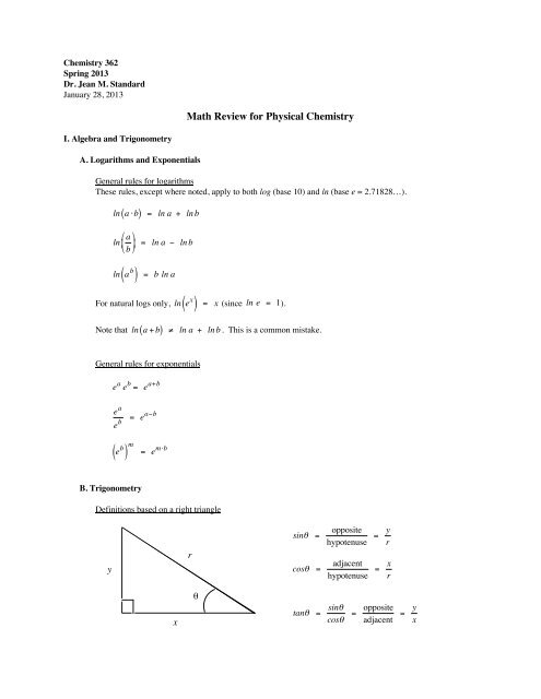
Definitions based on a right triangle
y
r
€
sinθ =
cosθ =
opposite
hypotenuse = y r
adjacent
hypotenuse
= x r
x
θ
€
tanθ = sinθ
cosθ
= opposite
adjacent
= y x
€

2
Other trigonometric function definitions
cotθ =
1
tanθ
= cosθ
sinθ
€
€
secθ =
cscθ =
1
cosθ
1
sinθ
€
Trigonometric Identities
sin 2 θ + cos 2 θ = 1
sin2θ = 2sinθ cosθ
€
cos2θ = cos 2 θ − sin 2 θ
€
II. Calculus [See also Mathematical Background 1 and 2 in your text.]
€
A. Derivatives
Derivatives of common functions
d
dx x n
= n x n−1
€
€
€
€
d
dx eax
= a e ax
d
dx ln x = 1 x
d
sin x = cos x
dx
d
cos x = − sin x
dx
€
€
€
€
General rules for manipulation of derivatives
d
dx c ⋅ f x
d
dx
d
dx
[ ( )]
= c ⋅ f ʹ′ ( x) (c is a constant)
[ f ( x)
+ g( x)
] =
[ f ( x)
⋅ g( x)
] = f x
d
dx f u x
( ( ))
= df
du ⋅ du
dx
d
dx f x ( ) + d dx g x ( )
( ) ⋅ g ʹ′ ( x) + g( x) ⋅ f ʹ′ ( x) (the Product Rule)
(the Chain Rule)
€

3
B. Integrals
Integrals of common functions
Note that since these are indefinite integrals, they all should include an overall constant of integration.
∫ x n dx =
1
n +1 x n+1
€
∫ e bx dx = 1 b ebx
€
1
∫
x dx = ln x
€
∫ sin x dx = − cos x
€
∫ cos x dx = sin x
€
€
General rules for manipulation of integrals
∫ c ⋅ f ( x) dx = c ⋅ f ( x) dx
∫
(c is a constant)
∫ [ f ( x) + g( x)
] dx = ∫ f ( x) dx + ∫ g x
( ) dx
€

4
Some More Definite and Indefinite Integrals
1.
∞
∫
0
e −bx
dx = 1 b
€
2.
∞
∫ x n e −bx dx =
0
n!
b n+1
€
3.
∞
∫ e −bx 2
dx = 1 2
0
⎛⎛ π ⎞⎞
⎜⎜ ⎟⎟
⎝⎝ b ⎠⎠
1
2
€
4.
∞
∫ x e −bx 2
dx =
0
1
2b
€
5.
∞
∫ x 2 e −bx 2
dx =
0
1 ⎛⎛ π ⎞⎞
⎜⎜ ⎟⎟
4b ⎝⎝ b ⎠⎠
1
2
€
6.
∫
sin 2 bx dx = x 2 − sin2bx
4b
€
7.
∫
x sin
bx dx = sinbx
b 2
− x cosbx
b
€
8.
∫ x sin 2 bx dx = x 2
4 − x sin2bx
4b
− cos2bx
8b 2
€
9.
∫
sin 3
bx dx = − cosbx
3b
[ sin 2 bx + 2]
€
10.
∫
sin
bx cosbx dx = sin2 bx
2b
€
11.
∫ cos 2 bx dx = x 2 + sin2bx
4b
€
Other sources for integrals: CRC handbooks and The Integrator at http://www.integrals.com.

5
III. A Guide to Complex Numbers
General Definitions
All complex numbers have at their root the imaginary number i,
Complex numbers are written as a real part and an imaginary part,
i = −1 . (1)
€
z = a + i b , (2)
where z is a complex number and a and b are real numbers. The number a is referred to as the real part of the
complex number, while the number b is referred to as the imaginary part since it is multiplied by i.
€
A function may also contain imaginary numbers. The simplest types of such functions can be divided into real and
imaginary parts,
f ( x) and
In this equation, g x
referred to as the real part of the function € h x
h( x) = f ( x) + i g( x) . (3)
( ) are real functions. As for the complex numbers defined in Equation (2), f ( x) is
( ) and g( x) is referred to as the imaginary part of the function g( x) .
€ €
€
Euler’s Relation
€ €
€
Functions that contain imaginary numbers may not always be easily separated into real and imaginary parts.
However, a typical function used in quantum mechanics has the imaginary number in the exponent,
f ( x) = e i k x , (4)
where k is a constant. Even this function may be separated into real and imaginary parts using Euler’s relation,
€
e i k x = cos kx + i sin kx . (5)
Complex Conjugates
€
An important quantity when dealing with complex numbers and functions is the complex conjugate. The complex
conjugate of a number or function that contains an imaginary part is obtained by replacing i by –i where it appears.
A complex conjugate is denoted by an asterisk. For example, for a complex number z, the complex conjugate is z*.
If z = a + i b, then the complex conjugate is
z * = a − i b. (6)
€
The complex conjugate of a function such as the one in Equation (3) is defined similarly,
€
h * ( x) = f ( x) − i g( x) . (7)
And, for the function given in Equation (4), the complex conjugate is
€
f * ( x) = e −i k x . (8)
€

6
Absolute Squares of Complex Variables
An important property of the complex conjugate of a number or a function is that when the complex conjugate is
multiplied by the original number or function, the result is always real and positive. For example, consider the
product of a complex number z and its complex conjugate, z ⋅ z *, which is known as the absolute square,
z ⋅ z * = ( a + i b) ( a − i b)
= a€
2 + i ab − iab − i 2 b 2
= a 2 − i 2 b 2
z ⋅ z * = a 2 + b 2 .
(9)
The above relation simplifies using the result that = −1. The complex conjugate multiplied by the original also
yields a real and positive result € for functions. For example, consider the function given in Equation (4),
i 2
€
f ( x) ⋅ f * ( x) = e i k x e −i k x
= e 0
f ( x) ⋅ f * ( x) = 1.
(10)
€
More information related to complex variables may be found in Mathematical Background 3 in your textbook.