Multipole moments - CRM2
Multipole moments - CRM2
Multipole moments - CRM2

Create successful ePaper yourself
Turn your PDF publications into a flip-book with our unique Google optimized e-Paper software.
Chapter 7<br />
<strong>Multipole</strong> expansion – Cartesian<br />
formalism<br />
The complete determination of the complete charge density and various response<br />
functions (and the associated deformation densities) is computationally heavy and<br />
conceptually not very rewarding. As any distribution function, the essential features<br />
of the charge distribution can be be characterized by its <strong>moments</strong>.<br />
The mathematical analogy between the Longuet-Higgins interaction operator and<br />
the electrostatic interaction energy allows us to generalize the results obtained for<br />
the latter to the interaction operator too.<br />
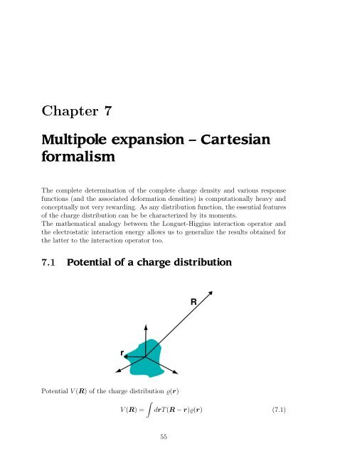
7.1 Potential of a charge distribution<br />
Potential V (R) of the charge distribution ϱ(r)<br />
∫<br />
V (R) = drT (R − r)ϱ(r) (7.1)<br />
55
can be expanded in Taylor series around r = 0 (|r| < |R|.<br />
Taylor expansion of the Coulomb kernel<br />
)<br />
)<br />
T (R − r) = 1 ( 1<br />
R − r α∇ α + 1 ( 1<br />
R 2! r αr β ∇ α ∇ β<br />
R<br />
− 1 ( ) 1<br />
3! r αr β r γ ∇ α ∇ β ∇ γ + . . .<br />
R<br />
(7.2)<br />
Define the (Cartesian) Coulomb interaction tensors<br />
T (R) = 1 R<br />
)<br />
T α (R) = ∇ α<br />
( 1<br />
R<br />
T αβ (R) = ∇ α ∇ β<br />
( 1<br />
R<br />
)<br />
)<br />
(7.3)<br />
T αβγ (R) = ∇ α ∇ β ∇ γ<br />
( 1<br />
R<br />
)<br />
T αβ...ν (R) = ∇ α ∇ β . . . ∇ ν<br />
( 1<br />
R<br />
and the electrostatic potential<br />
∫<br />
V (R) = T (R)<br />
∫<br />
drϱ(r) − T α (R) drr α ϱ(r)<br />
+ T αβ (R) 1 ∫<br />
drr α r β ϱ(r) − T αβγ (R) 1 ∫<br />
2!<br />
3!<br />
drr α r β r γ ϱ(r) + . . .<br />
(7.4)<br />
Define the multipole <strong>moments</strong> of the charge distribution<br />
∫<br />
q = drϱ(r)<br />
∫<br />
m α = drr α ϱ(r)<br />
∫<br />
Q αβ = drr α r β ϱ(r)<br />
(7.5)<br />
ξ αβ...ν = drr (n)<br />
αβ...ν ϱ(r)<br />
∫<br />
O αβγ = drr α r β r γ ϱ(r)<br />
∫<br />
Cartesian multipole expansion of the potential<br />
V (R) = qT (R) − m α T α (R) + 1 2! Q αβT αβ (R) − . . . + (−)n ξ αβ...ν T αβ...ν (R) (7.6)<br />
n!<br />
56
7.2 <strong>Multipole</strong> <strong>moments</strong><br />
There are several conventions in the literature. The above-defined multipole <strong>moments</strong><br />
are symmetric tensors Q αβ = Q βα and their trace is nonzero<br />
. ∑<br />
= Q αα ≠ 0 (7.7)<br />
Q αα<br />
They can be called “unnormalized traced Cartesian” multipoles.<br />
Unabridged multipoles (Applequist)<br />
Traceless cartesian multipoles (Buckingham)<br />
Potential of a quadrupole<br />
α<br />
µ αβ...ν = 1 n! ξ αβ...ν (7.8)<br />
V (2) (R) = 1 2 Q αβT αβ (R) (7.9)<br />
Since the T (R) = 1 function satisfies the Laplace equation<br />
R<br />
( ) 1<br />
∇ 2 = 0<br />
R<br />
∑<br />
( ) 1<br />
∇ α ∇ α = ∑ T αα (R) = 0<br />
R<br />
α<br />
α<br />
we can add to the quadrupole potential an arbitrary quantity<br />
(7.10)<br />
λδ αβ T αβ (R) (7.11)<br />
without changing its value<br />
V (2) (R) = 1 2 (Q αβ + λδ αβ ) T αβ (R) (7.12)<br />
Let us choose λ as the trace of Q αβ<br />
λ = − 1 3 Q αα = − 1 ∑<br />
Q αα (7.13)<br />
3<br />
The new expression of the quadrupole potential<br />
V (2) (R) = 1 2 · 1 ∫<br />
dr ( )<br />
3r α r β − r 2 δ αβ ϱ(r)Tαβ (R) = 1 3<br />
3 Θ αβT αβ (R) (7.14)<br />
where have introduced the traceless cartesian quadrupole moment<br />
Θ αβ = 1 ∫<br />
dr ( )<br />
3r α r β − r 2 δ αβ ϱ(r) (7.15)<br />
2<br />
α<br />
57
7.2.1 Traceless (Buckingham) multipole <strong>moments</strong><br />
General definition<br />
Electrostatic potential<br />
M (n)<br />
αβ...ν = (−)n<br />
n!<br />
V (R) = ∑ n<br />
where the notation (2n − 1)!! means<br />
∫<br />
( )<br />
drϱ(r)r 2n+1 ∂ n 1<br />
∂r α ∂ . . . r ν r<br />
(7.16)<br />
(−) n<br />
(2n − 1)!! M (n)<br />
αβ...ν T (n)<br />
αβ...ν<br />
(R) (7.17)<br />
(2n − 1)!! = 1 · 3 · 5 · . . . (2n − 1) (7.18)<br />
The traceless multipoles do not contain the full information about the ϱ(r) charge<br />
distribution, since they are undetermined up to an arbitrary spherically symmetric<br />
component.<br />
On the contrary, one can reconstruct the full charge density from the traced multipoles.<br />
Consider the Fourier transform of ϱ(r)<br />
∫<br />
ϱ(k) = dre ikr ϱ(r) (7.19)<br />
and expand the exponential<br />
∫<br />
∫<br />
ϱ(k) = drϱ(r) +ik α dr r α ϱ(r) − 1 ∫<br />
2! k αk β dr r α r β ϱ(r) + . . . (7.20)<br />
} {{ } } {{ } } {{ }<br />
q<br />
m α<br />
Q αβ<br />
7.2.2 Explicit form of higher multipole <strong>moments</strong><br />
◦ Quadrupole moment Θ αβ<br />
Θ αβ = ∑ a<br />
q a [ 3 2 a αa β − 1 2 a2 δ αβ ] (7.21)<br />
Six distinct components, five independent components.<br />
◦ Octopole moment Ω αβγ<br />
Ω αβγ = ∑ a<br />
q a [ 5 3 a αa β a γ − a 2 (a α δ βγ + a β δ γα + a γ δ αβ )] (7.22)<br />
10 distinct components, seven independent components.<br />
◦ Hexadecapole moment Φ αβγγ<br />
◦ 2 n <strong>moments</strong>...<br />
58
7.2.3 Translation of multipole <strong>moments</strong><br />
◦ Dipole moment of a point charge distribution<br />
µ α = ∑ i<br />
q i r i α (7.23)<br />
In a new frame obtained after a translation by a vector a<br />
µ ′ α = ∑ q i (rα i − a α ) = ∑ ∑<br />
q i rα i − a α q i = µ α − a α q tot (7.24)<br />
i<br />
i<br />
i<br />
Dipole of a neutral system (q tot = 0) is invariant to translation of origin.<br />
◦ Quadrupole moment<br />
Θ αβ = ∑ q ( )<br />
i 3rαr i β i − (r i ) 2 δ αβ (7.25)<br />
i<br />
After translation by a<br />
Θ ′ αβ = Θ αβ + 1 2 qtot (3a α a β − a 2 δ αβ )<br />
− 3 2 (µtot α a β + µ tot<br />
β a α ) − δ αβ µ tot<br />
α a α<br />
(7.26)<br />
7.3 Electric field, field gradient<br />
The electric field, field gradient<br />
F α (R) = −∇ α V (R) F αβ (R) = −∇ α ∇ β V (R) (7.27)<br />
and higher derivatives of the potential of a multipolar charge distribution can be<br />
expressed with the same interaction tensors<br />
F l 1<br />
α 1 ...ν 1<br />
= −∇ α . . . ∇ ν1 V (R) =<br />
∞∑ (−) l 2<br />
−<br />
(2l 2 − 1)!! T l 1+l 2<br />
α 1 ...ν 1 α 2 ...ν 2<br />
M l (7.28)<br />
2<br />
α 2 ...ν 2<br />
l 2<br />
7.4 Energy of a charge distribution in non-uniform<br />
field<br />
We choose the origin inside the charge distribution, ϱ(r) and expand the external<br />
potential in Taylor series around the origin<br />
V (r) = V (0) + r α V α (0) + 1 2! r αr β V αβ (0) + 1 3! r αr β r γ V αβγ (0) + . . . (7.29)<br />
59
Using the expression of the interaction energy<br />
∫<br />
∫<br />
∫<br />
U = drϱ(r)V (r) = drϱ(r)V (0) + drϱ(r)r α V α (0)<br />
+ 1 ∫<br />
drϱ(r)r α r β V αβ (0) + 1 ∫<br />
drϱ(r)r α r β r γ V αβγ (0) + . . .<br />
2!<br />
3!<br />
(7.30)<br />
where we recognize the definition of the unnormalized traced multipoles,<br />
U = MV + M α V α + 1 2! M αβV αβ + 1 3! M αβγV αβγ + . . . (7.31)<br />
By the virtue of the Laplace equation, V αα = 0, we can subtract the trace of M αβ ,<br />
i.e. 1 3 M αα from the quadrupolar energy<br />
1<br />
2 M αβV αβ = 1 2 V 1<br />
αβ(M αβ − δ αβ<br />
3 M αα) = 1 3 V αβΘ αβ (7.32)<br />
By similar manipulations at higher orders<br />
U = qV + µ α V α + 1 3 Θ αβV αβ + 1<br />
3 · 5 Ω αβγV αβγ<br />
1<br />
+<br />
3 · 5 · 7 Φ 1<br />
(7.33)<br />
αβγδV αβγδ +<br />
(2n − 1)!! ξ(n) α...νV α...ν<br />
The energy is the scalar product of the field with dipole, filed gradient with quadrupole<br />
and higher field gradients with the corresponding multipole tensors.<br />
Attention: the result may depend on the choice of origin!<br />
7.5 <strong>Multipole</strong> interaction energy<br />
Take two sets of multipoles. Taylor series of the Coulomb interaction<br />
1<br />
|τ − τ ′ | = 1<br />
|B + s − A − r| = 1<br />
|R − (r − s)| =<br />
= 1 ( ) 1<br />
R + (r α − s α )∇ α + 1 ( ) 1<br />
R 2! (r α − s α )(r β − s β )∇ α ∇ β + . . .<br />
R<br />
(7.34)<br />
which leads directly to an expression of the interaction energy of two multipole<br />
charge distributions in terms of their traced Cartesian <strong>moments</strong><br />
U(R) = q A q B T (R) + (m A αq B − q A m α )T α (R)<br />
+ 1 2! (QA αβq B + q A Q B αβ − m A αm B β − m B α m A β )T αβ (R) + . . .<br />
Using the traceless (Buckingham) <strong>moments</strong><br />
(7.35)<br />
U(R) = ∑ l 1 l 2<br />
(−) l 1<br />
(2l 1 − 1)!!(2l 2 − 1)!! M (l 1)[A]<br />
α 1 ...ν 1<br />
T (l 1+l 2 )<br />
α 1 ...ν 1 α 2 ...ν 2<br />
(R)M (l 2)[B]<br />
α 2 ...ν 2<br />
(7.36)<br />
60
7.6 Calculation of cartesian interaction tensors<br />
They are defined as<br />
T = 1 R = R−1 =<br />
1<br />
√ R<br />
2<br />
x + R 2 y + R 2 z<br />
(7.37)<br />
Using the following derivation “rules”<br />
∇ α R β = δ αβ ∇ α R n = nR α R (n−2) ∇ α R −n = −nR α R −(n+2) (7.38)<br />
◦ Charge-dipole<br />
T α (R) = ∇ α T (R) = −R α R −3 (7.39)<br />
◦ Dipole-dipole/charge-quadrupole<br />
T αβ (R) = ∇ α ∇ β T (R)<br />
= −∇ α R β R −3 = −δ αβ R −3 + 3R α R β R −5<br />
= (3R α R β − R 2 δ αβ )R −5 (7.40)<br />
◦ Dipole-quadrupole/charge-octopole<br />
T αβγ (R) = ∇ α ∇ β ∇ γ T (R) = δ α (3R β R γ − R 2 δ βγ )R −5<br />
= 3δ αβ R γ R −5 + 3δ αγ R β R −5 + 3δ βγ R α R −5 + 3 · 5 · R α R β R γ R −7<br />
= 3 ( 5R α R β R γ − R 2 (R α δ βγ + R β δ γα + R γ δ αβ ) ) R −7 (7.41)<br />
Interaction tensors<br />
◦ invariant to interchange of indices<br />
◦ traceless, since ∇ 2 (1/R) = 0<br />
◦ 2n+1 independent components<br />
Cartesian tensor formulation<br />
◦ simple in low orders<br />
◦ easily extended algorithms<br />
◦ global frame<br />
◦ heavy formalism<br />
◦ too much components (reducible<br />
and redundant)<br />
61
7.7 Example: Structure of the HX dimers<br />
Competition of three multipolar interaction. Angular dependence for linear molecules<br />
(symmetric tops) is the following<br />
◦ dipole-dipole<br />
◦ dipole-quadrupole<br />
U µµ = − µA µ B<br />
R 3 (2 cos θ A cos θ B − sin θ A sin θ B cos ϕ) (7.42)<br />
U µΘ = 3µA Θ B<br />
4R 4 [cos θ A (3 cos 2 θ B − 1) − sin θ A sin 2θ B cos ϕ] (7.43)<br />
◦ quadrupole-quadrupole<br />
U ΘΘ = ΘA Θ B<br />
R 5 3<br />
4 [1 − 5 cos2 θ A − 5 cos 2 θ B − 15 cos 2 θ A cos 2 θ B<br />
+ 2(4 cos θ A cos θ B − sin θ A sin θ B cos ϕ) 2 ]<br />
(7.44)<br />
The structure is characterized by θ A ≈ 0 and ϕ = 0, µ A = µ B = µ and Θ A = Θ B =<br />
Θ. The sum of the 4 interaction terms (two for U µΘ )<br />
U = − µ2<br />
R 3 · 2 cos θ<br />
+ µΘ<br />
R 4 · 3<br />
2 [(3 cos2 θ − 1) − 2 cos θ]<br />
+ Θ2<br />
R 5 · 3(3 cos2 θ − 1)<br />
(7.45)<br />
Introduce the parameter λ = Θ µR<br />
U = µ2<br />
R 3 {<br />
−2 cos θ + λ<br />
3<br />
2 [(3 cos2 θ − 1) − 2 cos θ] + λ 2 3(3 cos 2 θ − 1) }<br />
= µ2<br />
2R 3 {<br />
3λ(1 + 2λ)(3 cos 2 θ − 1) − 2(2 + 3λ) cos θ } (7.46)<br />
62
Electrostatic interaction energy<br />
is plotted for the<br />
◦ HF dimer<br />
µ = 0.72ea 0 ,<br />
Θ = 1.875ea 2 0<br />
R = 5.1a 0 ;<br />
minimum at 68 degrees<br />
(exp. 60)<br />
◦ HCl dimer<br />
µ = 0.433ea 0 ,<br />
Θ = 2.8ea 2 0<br />
R = 6.8a 0 ;<br />
minimum at 79 degrees<br />
63