PSTricks pst-fractal
PSTricks pst-fractal
PSTricks pst-fractal

Create successful ePaper yourself
Turn your PDF publications into a flip-book with our unique Google optimized e-Paper software.
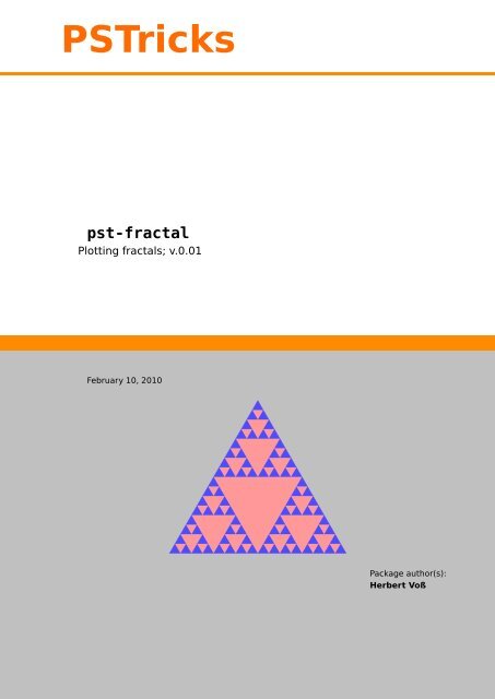
<strong>PSTricks</strong><br />
<strong>pst</strong>-<strong>fractal</strong><br />
Plotting <strong>fractal</strong>s; v.0.01<br />
February 10, 2010<br />
Package author(s):<br />
Herbert Voß
Contents 2<br />
Contents<br />
1 Sierpinski triangle 4<br />
2 Julia and Mandelbrot sets 4<br />
2.1 Julia sets . . . . . . . . . . . . . . . . . . . . . . . . . . . . . . . . . . . . . . . 5<br />
2.2 Mandelbrot sets . . . . . . . . . . . . . . . . . . . . . . . . . . . . . . . . . . . 5<br />
2.3 The options . . . . . . . . . . . . . . . . . . . . . . . . . . . . . . . . . . . . . 6<br />
2.4 type . . . . . . . . . . . . . . . . . . . . . . . . . . . . . . . . . . . . . . . . . 6<br />
2.5 baseColor . . . . . . . . . . . . . . . . . . . . . . . . . . . . . . . . . . . . . . 6<br />
2.6 xWidth and yWidth . . . . . . . . . . . . . . . . . . . . . . . . . . . . . . . . . 6<br />
2.7 cx and cy . . . . . . . . . . . . . . . . . . . . . . . . . . . . . . . . . . . . . . . 7<br />
2.8 dIter . . . . . . . . . . . . . . . . . . . . . . . . . . . . . . . . . . . . . . . . . 7<br />
2.9 maxIter . . . . . . . . . . . . . . . . . . . . . . . . . . . . . . . . . . . . . . . 7<br />
2.10maxRadius . . . . . . . . . . . . . . . . . . . . . . . . . . . . . . . . . . . . . . 7<br />
2.11plotpoints . . . . . . . . . . . . . . . . . . . . . . . . . . . . . . . . . . . . . 8<br />
3 Phyllotaxis 8<br />
3.1 angle . . . . . . . . . . . . . . . . . . . . . . . . . . . . . . . . . . . . . . . . . 9<br />
3.2 c . . . . . . . . . . . . . . . . . . . . . . . . . . . . . . . . . . . . . . . . . . . 9<br />
3.3 maxIter . . . . . . . . . . . . . . . . . . . . . . . . . . . . . . . . . . . . . . . 10<br />
4 Fern 11<br />
5 Koch flake 12<br />
6 Apollonius circles 13<br />
7 Trees 14<br />
8 List of all optional arguments for <strong>pst</strong>-<strong>fractal</strong> 16
The well known <strong>pst</strong>ricks package offers excellent macros to insert more or less complex<br />
graphics into a document. <strong>pst</strong>ricks itself is the base for several other additional<br />
packages, which are mostly named <strong>pst</strong>-xxxx, like <strong>pst</strong>-<strong>fractal</strong>.<br />
This version uses the extended keyval package xkeyval, so be sure that you have installed<br />
this package together with the spcecial one <strong>pst</strong>-xkey for <strong>PSTricks</strong>. The xkeyval<br />
package is available at CTAN:/macros/latex/contrib/xkeyval/. It is also important<br />
that after <strong>pst</strong>-<strong>fractal</strong> no package is loaded, which uses the old keyval interface.<br />
The <strong>fractal</strong>s are really big, which is the reason why this document is about 15 MByte<br />
when you run it without using the external png-images.
1 Sierpinski triangle 4<br />
All images in this documentation were converted to the .jpg format to get a small pdf<br />
file size. When using the pdf format for the images the file size will be more than 20<br />
MBytes. However, having a small file size will lead into a bad image resolution. Run the<br />
examples as single documents to see how it will be in high quality.<br />
1 Sierpinski triangle<br />
The triangle must be given by three mandatory arguments. Depending to the kind of<br />
arguments it is one of the two possible versions:<br />
\psSier [Options] (x 0 ,y 0 )(x 1 ,y 1 )(x 2 ,y 2 )<br />
\psSier [Options] (x 0 ,y 0 ){Base}{Recursion}<br />
In difference to \ps<strong>fractal</strong> it doesn’t reserve any space, this is the reason why it should<br />
be part of a pspicture environment.<br />
1\begin{pspicture}(5,5)<br />
2 \psSier(0,0)(2,5)(5,0)<br />
3\end{pspicture}<br />
1\begin{pspicture}(5,5)<br />
2\psSier[linecolor=blue!70,<br />
3 fillcolor=red!40](0,0){5cm}{4}<br />
4\end{pspicture}<br />
2 Julia and Mandelbrot sets<br />
The syntax of the \ps<strong>fractal</strong> macro is simple<br />
\ps<strong>fractal</strong> [Options] (x 0 ,y 0 )(x 1 ,y 1 )<br />
All Arguments are optional, \ps<strong>fractal</strong> is the same as \ps<strong>fractal</strong>(-1,-1)(1,1). The<br />
Julia and Mandelbrot sets are a graphical representation of the following sequence x is<br />
the real and y the imaginary part of the complex number z. C(x, y) is a complex constant
2.1 Julia sets 5<br />
and preset by (0, 0).<br />
z n+1 (x, y) = (z n (x, y)) 2 + C(x, y) (1)<br />
2.1 Julia sets<br />
A Julia set is given with<br />
z n+1 (x, y) = (z n (x, y)) 2 + C(x, y) (2)<br />
z 0 = (x 0 ; y 0 ) (3)<br />
(x 0 ; y 0 ) is the starting value.<br />
1\pspicture(-1,-1)(1,1)\ps<strong>fractal</strong>\<br />
endpspicture<br />
1\pspicture(-2,-2)(2,2)<br />
2\ps<strong>fractal</strong>[xWidth=4cm,yWidth=4cm,<br />
baseColor=white, dIter=20](-2,-2)<br />
(2,2)<br />
3\endpspicture<br />
2.2 Mandelbrot sets<br />
A Mandelbrot set is given with<br />
z n+1 (x, y) = (z n (x, y)) 2 + C(x, y) (4)<br />
z 0 = (0; 0) (5)<br />
C(x, y) = (x 0 ; y 0 ) (6)<br />
(x 0 ; y 0 ) is the starting value.<br />
1\pspicture(-1,-1)(1,1)<br />
2\ps<strong>fractal</strong>[type=Mandel]<br />
3\endpspicture
2.3 The options 6<br />
1\pspicture(-2,-2)(2,2)<br />
2\ps<strong>fractal</strong>[type=Mandel, xWidth=6cm,<br />
3 yWidth=4.8cm, baseColor=white,<br />
4 dIter=10](-2,-1.2)(1,1.2)<br />
5\endpspicture<br />
2.3 The options<br />
2.4 type<br />
txpe can be of Julia (default) or Mandel.<br />
1\pspicture(-1,-1)(3,1)<br />
2\ps<strong>fractal</strong><br />
3\ps<strong>fractal</strong>[type=Mandel]<br />
4\endpspicture<br />
2.5 baseColor<br />
The color for the convergent part is set by baseColor.<br />
1\begin{postscript}<br />
2\ps<strong>fractal</strong>[xWidth=4cm,yWidth=4cm,dIter<br />
=30](-2,-2)(2,2)<br />
3\ps<strong>fractal</strong>[xWidth=4cm,yWidth=4cm,<br />
baseColor=yellow,dIter=30](-2,-2)<br />
(2,2)<br />
4\end{postscript}<br />
2.6 xWidth and yWidth<br />
xWidth and yWidth define the physical width of the <strong>fractal</strong>.<br />
1\begin{postscript}<br />
2\ps<strong>fractal</strong>[type=Mandel,xWidth=12.8cm,<br />
yWidth=10.8cm,dIter=5](-2.5,-1.3)<br />
(0.7,1.3)<br />
3\end{postscript}
2.7 cx and cy 7<br />
2.7 cx and cy<br />
Define the starting value for the complex constant number C.<br />
1\begin{postscript}<br />
2\psset{xWidth=5cm,yWidth=5cm}<br />
3\ps<strong>fractal</strong>[dIter=2](-2,-2)(2,2)<br />
4\ps<strong>fractal</strong>[dIter=2,cx=-1.3,cy=0](-2,-2)<br />
(2,2)<br />
5\end{postscript}<br />
2.8 dIter<br />
The color is set by wavelength to RGB conversion of the iteration number, where dIter<br />
is the step, predefined by 1. The wavelength is given by the value of iter added by 400.<br />
1\begin{postscript}<br />
2\psset{xWidth=5cm,yWidth=5cm}<br />
3\ps<strong>fractal</strong>[dIter=30](-2,-2)(2,2)<br />
4\ps<strong>fractal</strong>[dIter=10,cx=-1.3,cy=0](-2,-2)<br />
(2,2)<br />
5\end{postscript}<br />
2.9 maxIter<br />
maxIter is the number of the maximum iteration until it leaves the loop. It is predefined<br />
by 255, but internally multiplied by dIter.<br />
1\begin{postscript}<br />
2\psset{xWidth=5cm,yWidth=5cm}<br />
3\ps<strong>fractal</strong>[maxIter=50,dIter=3](-2,-2)<br />
(2,2)<br />
4\ps<strong>fractal</strong>[maxIter=30,cx=-1.3,cy<br />
=0](-2,-2)(2,2)<br />
5\end{postscript}<br />
2.10 maxRadius<br />
If the square of distance of z n to the origin of the complex coordinate system is greater<br />
as maxRadius then the algorithm leaves the loop and sets the point. maxRadius should<br />
always be the square of the "‘real"’ value, it is preset by 100.
2.11 plotpoints 8<br />
1\begin{postscript}<br />
2\psset{xWidth=5cm,yWidth=5cm}<br />
3\ps<strong>fractal</strong>[maxRadius=30,dIter=10](-2,-2)<br />
(2,2)<br />
4\ps<strong>fractal</strong>[maxRadius=30,dIter=30,cx=-1.3,<br />
cy=0](-2,-2)(2,2)<br />
5\end{postscript}<br />
2.11 plotpoints<br />
This option is only valid for the Sierpinski triangle and preset by 2000.<br />
1\begin{pspicture}(5,5)<br />
2 \psSier[plotpoints=10000](0,0)(2.5,5)<br />
(5,0)<br />
3\end{pspicture}<br />
3 Phyllotaxis<br />
The beautiful arrangement of leaves in some plants, called phyllotaxis, obeys a number<br />
of subtle mathematical relationships. For instance, the florets in the head of a sunflower<br />
form two oppositely directed spirals: 55 of them clockwise and 34 counterclockwise.<br />
Surprisingly, these numbers are consecutive Fibonacci numbers. The Phyllotaxis is like<br />
a Lindenmayer system.<br />
\psPhyllotaxis [Options] (x,y)<br />
The coordinates of the center are optional, if they are missing, then (0, 0) is assumed.<br />
1\begin{postscript}<br />
2\psframebox{\begin{pspicture}(-3,-3)(3,3)<br />
3 \psPhyllotaxis<br />
4\end{pspicture}}<br />
5\end{postscript}
3.1 angle 9<br />
1\begin{postscript}<br />
2\psframebox{\begin{pspicture}(-3,-3)(4,4)<br />
3 \psPhyllotaxis(1,1)<br />
4\end{pspicture}}<br />
5\end{postscript}<br />
3.1 angle<br />
1\begin{postscript}<br />
2\psframebox{\begin{pspicture}(-2.5,-2.5)<br />
(2.5,2.5)<br />
3 \psPhyllotaxis[angle=99]<br />
4\end{pspicture}}<br />
5\end{postscript}<br />
3.2 c<br />
This is the length of one element in the unit pt.
3.3 maxIter 10<br />
1\begin{postscript}<br />
2\psframebox{\begin{pspicture}(8,8)<br />
3 \psPhyllotaxis[c=7](4,4)<br />
4\end{pspicture}}<br />
5\end{postscript}<br />
1\begin{postscript}<br />
2\psframebox{\begin{pspicture}(-3,-3)(3,3)<br />
3 \psPhyllotaxis[c=4,angle=111]<br />
4\end{pspicture}}<br />
5\end{postscript}<br />
3.3 maxIter<br />
This is the number for the iterations.<br />
1\begin{postscript}<br />
2\psframebox{\begin{pspicture}(-3,-3)(3,3)<br />
3 \psPhyllotaxis[c=6,angle=111,maxIter<br />
=100]<br />
4\end{pspicture}}<br />
5\end{postscript}
4 Fern 11<br />
4 Fern<br />
\psFern [Options] (x,y)<br />
The coordinates of the starting point are optional, if they are missing, then (0, 0) is<br />
assumed. The default scale is set to 10.<br />
1\begin{postscript}<br />
2\psframebox{\begin{pspicture}(-1,0)(1,4)<br />
3 \psFern<br />
4\end{pspicture}}<br />
5\end{postscript}<br />
1\begin{postscript}<br />
2\psframebox{\begin{pspicture}(-1,0)(2,5)<br />
3 \psFern(1,1)<br />
4\end{pspicture}}<br />
5\end{postscript}
5 Koch flake 12<br />
1\begin{postscript}<br />
2\psframebox{\begin{pspicture}(-3,0)(3,11)<br />
3 \psFern[scale=30,maxIter=100000,<br />
linecolor=green]<br />
4\end{pspicture}}<br />
5\end{postscript}<br />
5 Koch flake<br />
\psKochflake [Options] (x,y)<br />
The coordinates of the starting point are optional, if they are missing, then (0, 0) is<br />
assumed. The origin is the lower left point of the flake, marked as red or black point in<br />
the following example:<br />
1\begin{pspicture}[showgrid=true<br />
](-2.4,-0.4)(5,5)<br />
2 \psKochflake[scale=10]<br />
3 \psdot[linecolor=red,dotstyle=*](0,0)<br />
4\end{pspicture}
6 Apollonius circles 13<br />
1\begin{pspicture}(-0.4,-0.4)(12,4)<br />
2 \psset{fillcolor=lime,fillstyle=solid}<br />
3 \multido{\iA=0+1,\iB=0+2}{6}{%<br />
4 \psKochflake[angle=-30,scale=3,maxIter<br />
=\iA](\iB,2.5)\psdot*(\iB,2.5)<br />
5 \psKochflake[scale=3,maxIter=\iA](\iB<br />
,0)\psdot*(\iB,0)}<br />
6\end{pspicture}<br />
Optional arguments are scale, maxIter (iteration depth) and angle for the first rotation<br />
angle.<br />
6 Apollonius circles<br />
\psAppolonius [Options] (x,y)<br />
The coordinates of the starting point are optional, if they are missing, then (0, 0) is<br />
assumed. The origin is the center of the circle:<br />
1\begin{pspicture}[showgrid=true](-4,-4)<br />
(4,4)<br />
2 \psAppolonius[Radius=4cm]<br />
3\end{pspicture}
7 Trees 14<br />
1\begin{pspicture}(-5,-5)(5,5)<br />
2 \psAppolonius[Radius=5cm,Color]<br />
3\end{pspicture}<br />
7 Trees<br />
\psPTree [Options] (x,y) \psFArrow [Options] (x,y){fraction}<br />
The coordinates of the starting point are optional, if they are missing, then (0, 0) is<br />
assumed. The origin is the center of the lower line, shown in the following examples by<br />
the dot. Special parameters are the width of the lower basic line for the tree and the<br />
height and angle for the arrow and for both the color option. The color step is given by<br />
dIter and the depth by maxIter. Valid optional arguments are<br />
Name Meaning default<br />
xWidth first base width 1cm<br />
minWidth last base width 1pt<br />
c factor for unbalanced trees (0
7 Trees 15<br />
1\begin{pspicture}[showgrid=true](-6,0)<br />
(6,7)<br />
2 \psPTree[xWidth=1.75cm,Color=true]<br />
3 \psdot*[linecolor=white](0,0)<br />
4\end{pspicture}<br />
1\begin{pspicture}(-7,-1)(6,8)<br />
2 \psPTree[xWidth=1.75cm,c=0.35]<br />
3\end{pspicture}<br />
1\begin{pspicture}(-5,-1)(7,8)<br />
2 \psPTree[xWidth=1.75cm,Color=true,c<br />
=0.65]<br />
3\end{pspicture}<br />
1\begin{pspicture*}[showgrid=true](-3,0)<br />
(3,3.5)<br />
2 \psFArrow[linewidth=3pt]{0.65}<br />
3\end{pspicture*}<br />
1\begin{pspicture*}(-3,0)(3,3.5)<br />
2 \psFArrow[Color]{0.65}<br />
3\end{pspicture*}
References 16<br />
1\begin{pspicture*}(-4,-3)(3,3)<br />
2 \psFArrow[Color]{0.7}<br />
3 \psFArrow[angle=90,Color]{0.7}<br />
4\end{pspicture*}<br />
8 List of all optional arguments for <strong>pst</strong>-<strong>fractal</strong><br />
Key Type Default<br />
xWidth ordinary 1cm<br />
yWidth ordinary 1cm<br />
type ordinary Julia<br />
baseColor ordinary white<br />
cx ordinary 0<br />
cy ordinary 0<br />
dIter ordinary 1<br />
maxIter ordinary 255<br />
maxRadius ordinary 100<br />
plotpoints ordinary 2000<br />
angle ordinary 0<br />
c ordinary 5<br />
minWidth ordinary 1pt<br />
scale ordinary 1<br />
Radius ordinary 5cm<br />
Color boolean true<br />
References<br />
[1] Michel Goosens, Frank Mittelbach, Sebastian Rahtz, Denis Roegel, and Herbert<br />
Voß. The L A T E X Graphics Companion. Addison-Wesley Publishing Company,<br />
Reading, Mass., 2007.<br />
[2] Laura E. Jackson and Herbert Voß. Die Plot-Funktionen von <strong>pst</strong>-plot. Die<br />
T E Xnische Komödie, 2/02:27–34, June 2002.<br />
[3] Nikolai G. Kollock. PostScript richtig eingesetzt: vom Konzept zum praktischen<br />
Einsatz. IWT, Vaterstetten, 1989.<br />
[4] Manuel Luque. Vue en 3D.<br />
http://members.aol.com/Mluque5130/vue3d16112002.zip, 2002.<br />
[5] Herbert Voß. Die mathematischen Funktionen von Postscript. Die T E Xnische<br />
Komödie, 1/02:40–47, March 2002.
References 17<br />
[6] Herbert Voss. <strong>PSTricks</strong> Support for pdf.<br />
http://<strong>PSTricks</strong>.de/pdf/pdfoutput.phtml, 2002.<br />
[7] Herbert Voß. L A T E X in Mathematik und Naturwissenschaften. Franzis-Verlag,<br />
Poing, 2006.<br />
[8] Herbert Voß. <strong>PSTricks</strong> – Grafik für T E X und L A T E X. DANTE – Lehmanns,<br />
Heidelberg/Hamburg, 4. edition, 2007.<br />
[9] Michael Wiedmann and Peter Karp. References for T E X and Friends.<br />
http://www.miwie.org/tex-refs/, 2003.<br />
[10] Timothy Van Zandt. <strong>PSTricks</strong> - PostScript macros for Generic TeX.<br />
http://www.tug.org/application/<strong>PSTricks</strong>, 1993.
Index<br />
angle, 9, 13<br />
baseColor, 6<br />
c, 9, 14<br />
Color, 14<br />
cx, 7<br />
cy, 7<br />
dIter, 7, 14<br />
Environment<br />
pspicture, 4<br />
Extension<br />
.jpg, 4<br />
iter, 7<br />
.jpg, 4<br />
Julia, 6<br />
Keyvalue<br />
Julia, 6<br />
Mandel, 6<br />
Keyword<br />
angle, 9, 13<br />
baseColor, 6<br />
c, 9, 14<br />
Color, 14<br />
cx, 7<br />
cy, 7<br />
dIter, 7, 14<br />
maxIter, 7, 10, 13, 14<br />
maxRadius, 7<br />
minWidth, 14<br />
plotpoints, 8<br />
scale, 11, 13<br />
txpe, 6<br />
xWidth, 6, 14<br />
yWidth, 6<br />
Macro<br />
\psAppolonius, 13<br />
\psFArrow, 14<br />
\psFern, 11<br />
\ps<strong>fractal</strong>, 4<br />
\psKochflake, 12<br />
\psPhyllotaxis, 8<br />
\psPTree, 14<br />
\psSier, 4<br />
Mandel, 6<br />
maxIter, 7, 10, 13, 14<br />
maxRadius, 7<br />
minWidth, 14<br />
Package<br />
<strong>pst</strong>-<strong>fractal</strong>, 3<br />
<strong>pst</strong>-xkey, 3<br />
<strong>pst</strong>ricks, 3<br />
xkeyval, 3<br />
plotpoints, 8<br />
PostScript<br />
iter, 7<br />
\psAppolonius, 13<br />
\psFArrow, 14<br />
\psFern, 11<br />
\ps<strong>fractal</strong>, 4<br />
\psKochflake, 12<br />
\psPhyllotaxis, 8<br />
pspicture, 4<br />
\psPTree, 14<br />
\psSier, 4<br />
<strong>pst</strong>-<strong>fractal</strong>, 3<br />
<strong>pst</strong>-xkey, 3<br />
<strong>pst</strong>ricks, 3<br />
scale, 11, 13<br />
txpe, 6<br />
wavelength, 7<br />
xkeyval, 3<br />
xWidth, 6, 14<br />
yWidth, 6<br />
18