chapter one the estimation of physical properties

http://72.3.142.35/mghdxreader/jsp/print/FinalDisplayForPrint.jsp;jses... 

de 1 24/4/2006 10:00 

The Properties of Gases and Liquids, Fifth Edition Bruce E. Poling, John 

M. Prausnitz, John P. O’Connell 

cover 

Printed from Digital Engineering Library @ McGraw-Hill 

(www.Digitalengineeringlibrary.com). 

Copyright ©2004 The McGraw-Hill Companies. All rights reserved. 

Any use is subject to the Terms of Use as given at the website. 

>>

Source: THE PROPERTIES OF GASES AND LIQUIDS 

CHAPTER ONE 

THE ESTIMATION OF PHYSICAL 

PROPERTIES 

1-1 INTRODUCTION 

The structural engineer cannot design a bridge without knowing the properties of 

steel and concrete. Similarly, scientists and engineers often require the properties 

of gases and liquids. The chemical or process engineer, in particular, finds knowledge 

of physical properties of fluids essential to the design of many kinds of products, 

processes, and industrial equipment. Even the theoretical physicist must occasionally 

compare theory with measured properties. 

The physical properties of every substance depend directly on the nature of the 

molecules of the substance. Therefore, the ultimate generalization of physical properties 

of fluids will require a complete understanding of molecular behavior, which 

we do not yet have. Though its origins are ancient, the molecular theory was not 

generally accepted until about the beginning of the nineteenth century, and even 

then there were setbacks until experimental evidence vindicated the theory early in 

the twentieth century. Many pieces of the puzzle of molecular behavior have now 

fallen into place and computer simulation can now describe more and more complex 

systems, but as yet it has not been possible to develop a complete generalization. 

In the nineteenth century, the observations of Charles and Gay-Lussac were 

combined with Avogadro’s hypothesis to form the gas ‘‘law,’’ PV NRT, which 

was perhaps the first important correlation of properties. Deviations from the idealgas 

law, though often small, were finally tied to the fundamental nature of the 

molecules. The equation of van der Waals, the virial equation, and other equations 

of state express these quantitatively. Such extensions of the ideal-gas law have not 

only facilitated progress in the development of a molecular theory but, more important 

for our purposes here, have provided a framework for correlating physical 

properties of fluids. 

The original ‘‘hard-sphere’’ kinetic theory of gases was a significant contribution 

to progress in understanding the statistical behavior of a system containing a large 

number of molecules. Thermodynamic and transport properties were related quantitatively 

to molecular size and speed. Deviations from the hard-sphere kinetic theory 

led to studies of the interactions of molecules based on the realization that 

molecules attract at intermediate separations and repel when they come very close. 

The semiempirical potential functions of Lennard-Jones and others describe attraction 

and repulsion in approximately quantitative fashion. More recent potential 

functions allow for the shapes of molecules and for asymmetric charge distribution 

in polar molecules. 

1.1 

Downloaded from Digital Engineering Library @ McGraw-Hill (www.digitalengineeringlibrary.com) 

Copyright © 2004 The McGraw-Hill Companies. All rights reserved. 

Any use is subject to the Terms of Use as given at the website.

THE ESTIMATION OF PHYSICAL PROPERTIES 

1.2 CHAPTER ONE 

Although allowance for the forces of attraction and repulsion between molecules 

is primarily a development of the twentieth century, the concept is not new. In 

about 1750, Boscovich suggested that molecules (which he referred to as atoms) 

are ‘‘endowed with potential force, that any two atoms attract or repel each other 

with a force depending on their distance apart. At large distances the attraction 

varies as the inverse square of the distance. The ultimate force is a repulsion which 

increases without limit as the distance decreases without limit, so that the two atoms 

can never coincide’’ (Maxwell 1875). 

From the viewpoint of mathematical physics, the development of a comprehensive 

molecular theory would appear to be complete. J. C. Slater (1955) observed 

that, while we are still seeking the laws of nuclear physics, ‘‘in the physics of 

atoms, molecules and solids, we have found the laws and are exploring the deductions 

from them.’’ However, the suggestion that, in principle (the Schrödinger equation 

of quantum mechanics), everything is known about molecules is of little comfort 

to the engineer who needs to know the properties of some new chemical to 

design a commercial product or plant. 

Paralleling the continuing refinement of the molecular theory has been the development 

of thermodynamics and its application to properties. The two are intimately 

related and interdependent. Carnot was an engineer interested in steam engines, 

but the second law of thermodynamics was shown by Clausius, Kelvin, 

Maxwell, and especially by Gibbs to have broad applications in all branches of 

science. 

Thermodynamics by itself cannot provide physical properties; only molecular 

theory or experiment can do that. But thermodynamics reduces experimental or 

theoretical efforts by relating one physical property to another. For example, the 

Clausius-Clapeyron equation provides a useful method for obtaining enthalpies of 

vaporization from more easily measured vapor pressures. 

The second law led to the concept of chemical potential which is basic to an 

understanding of chemical and phase equilibria, and the Maxwell relations provide 

ways to obtain important thermodynamic properties of a substance from PVTx relations 

where x stands for composition. Since derivatives are often required, the 

PVTx function must be known accurately. 

The Information Age is providing a ‘‘shifting paradigm in the art and practice 

of physical properties data’’ (Dewan and Moore, 1999) where searching the World 

Wide Web can retrieve property information from sources and at rates unheard of 

a few years ago. Yet despite the many handbooks and journals devoted to compilation 

and critical review of physical-property data, it is inconceivable that all desired 

experimental data will ever be available for the thousands of compounds of 

interest in science and industry, let alone all their mixtures. Thus, in spite of impressive 

developments in molecular theory and information access, the engineer 

frequently finds a need for physical properties for which no experimental data are 

available and which cannot be calculated from existing theory. 

While the need for accurate design data is increasing, the rate of accumulation 

of new data is not increasing fast enough. Data on multicomponent mixtures are 

particularly scarce. The process engineer who is frequently called upon to design 

a plant to produce a new chemical (or a well-known chemical in a new way) often 

finds that the required physical-property data are not available. It may be possible 

to obtain the desired properties from new experimental measurements, but that is 

often not practical because such measurements tend to be expensive and timeconsuming. 

To meet budgetary and deadline requirements, the process engineer 

almost always must estimate at least some of the properties required for design. 





THE ESTIMATION OF PHYSICAL PROPERTIES 1.3 

1-2 ESTIMATION OF PROPERTIES 

In the all-too-frequent situation where no experimental value of the needed property 

is at hand, the value must be estimated or predicted. ‘‘Estimation’’ and ‘‘prediction’’ 

are often used as if they were synonymous, although the former properly carries 

the frank implication that the result may be only approximate. Estimates may be 

based on theory, on correlations of experimental values, or on a combination of 

both. A theoretical relation, although not strictly valid, may nevertheless serve adequately 

in specific cases. 

For example, to relate mass and volumetric flow rates of air through an airconditioning 

unit, the engineer is justified in using PV NRT. Similarly, he or she 

may properly use Dalton’s law and the vapor pressure of water to calculate the 

mass fraction of water in saturated air. However, the engineer must be able to judge 

the operating pressure at which such simple calculations lead to unacceptable error. 

Completely empirical correlations are often useful, but one must avoid the temptation 

to use them outside the narrow range of conditions on which they are based. 

In general, the stronger the theoretical basis, the more reliable the correlation. 

Most of the better estimation methods use equations based on the form of an 

incomplete theory with empirical correlations of the parameters that are not provided 

by that theory. Introduction of empiricism into parts of a theoretical relation 

provides a powerful method for developing a reliable correlation. For example, the 

van der Waals equation of state is a modification of the simple PV NRT; setting 

N 1, 

 

 

a 

P (V b) RT (1-2.1) 

V 2 

Equation (1-2.1) is based on the idea that the pressure on a container wall, exerted 

by the impinging molecules, is decreased because of the attraction by the mass of 

molecules in the bulk gas; that attraction rises with density. Further, the available 

space in which the molecules move is less than the total volume by the excluded 

volume b due to the size of the molecules themselves. Therefore, the ‘‘constants’’ 

(or parameters) a and b have some theoretical basis though the best descriptions 

require them to vary with conditions, that is, temperature and density. The correlation 

of a and b in terms of other properties of a substance is an example of the 

use of an empirically modified theoretical form. 

Empirical extension of theory can often lead to a correlation useful for estimation 

purposes. For example, several methods for estimating diffusion coefficients in lowpressure 

binary gas systems are empirical modifications of the equation given by 

the simple kinetic theory for non-attracting spheres. Almost all the better estimation 

procedures are based on correlations developed in this way. 

1-3 TYPES OF ESTIMATION 

An ideal system for the estimation of a physical property would (1) provide reliable 

physical and thermodynamic properties for pure substances and for mixtures at any 

temperature, pressure, and composition, (2) indicate the phase (solid, liquid, or gas), 

(3) require a minimum of input data, (4) choose the least-error route (i.e., the best 






estimation method), (5) indicate the probable error, and (6) minimize computation 

time. Few of the available methods approach this ideal, but some serve remarkably 

well. Thanks to modern computers, computation time is usually of little concern. 

In numerous practical cases, the most accurate method may not be the best for 

the purpose. Many engineering applications properly require only approximate estimates, 

and a simple estimation method requiring little or no input data is often 

preferred over a complex, possibly more accurate correlation. The simple gas law 

is useful at low to modest pressures, although more accurate correlations are available. 

Unfortunately, it is often not easy to provide guidance on when to reject the 

simpler in favor of the more complex (but more accurate) method; the decision 

often depends on the problem, not the system. 

Although a variety of molecular theories may be useful for data correlation, 

there is one theory which is particularly helpful. This theory, called the law of 

corresponding states or the corresponding-states principle, was originally based on 

macroscopic arguments, but its modern form has a molecular basis. 

The Law of Corresponding States 

Proposed by van der Waals in 1873, the law of corresponding states expresses the 

generalization that equilibrium properties that depend on certain intermolecular 

forces are related to the critical properties in a universal way. Corresponding states 

provides the single most important basis for the development of correlations and 

estimation methods. In 1873, van der Waals showed it to be theoretically valid for 

all pure substances whose PVT properties could be expressed by a two-constant 

equation of state such as Eq. (1-2.1). As shown by Pitzer in 1939, it is similarly 

valid if the intermolecular potential function requires only two characteristic parameters. 

Corresponding states holds well for fluids containing simple molecules 

and, upon semiempirical extension with a single additional parameter, it also holds 

for ‘‘normal’’ fluids where molecular orientation is not important, i.e., for molecules 

that are not strongly polar or hydrogen-bonded. 

The relation of pressure to volume at constant temperature is different for different 

substances; however, two-parameter corresponding states theory asserts that 

if pressure, volume, and temperature are divided by the corresponding critical properties, 

the function relating reduced pressure to reduced volume and reduced temperature 

becomes the same for all substances. The reduced property is commonly 

expressed as a fraction of the critical property: P r P/P c ; V r V/V c ; and T r 

T/T c . 

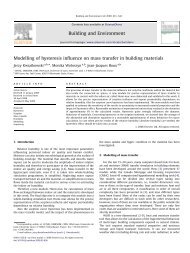
To illustrate corresponding states, Fig. 1-1 shows reduced PVT data for methane 

and nitrogen. In effect, the critical point is taken as the origin. The data for saturated 

liquid and saturated vapor coincide well for the two substances. The isotherms 

(constant T r ), of which only one is shown, agree equally well. 

Successful application of the law of corresponding states for correlation of PVT 

data has encouraged similar correlations of other properties that depend primarily 

on intermolecular forces. Many of these have proved valuable to the practicing 

engineer. Modifications of the law are commonly made to improve accuracy or ease 

of use. Good correlations of high-pressure gas viscosity have been obtained by 

expressing / c as a function of P r and T r . But since c is seldom known and not 

easily estimated, this quantity has been replaced in other correlations by other 

1/2 2/3 1/6 

characteristics such as , c T, or the group M Pc T c , where c is the viscosity 

at T c and low pressure, T is the viscosity at the temperature of interest, again at 






FIGURE 1-1 The law of corresponding states applied to the PVT 

properties of methane and nitrogen. Literature values (Din, 1961): 

methane, ● nitrogen. 

low pressure, and the group containing M, P c , and T c is suggested by dimensional 

analysis. Other alternatives to the use of c might be proposed, each modeled on 

the law of corresponding states but essentially empirical as applied to transport 

properties. 

The two-parameter law of corresponding states can be derived from statistical 

mechanics when severe simplifications are introduced into the partition function. 

Sometimes other useful results can be obtained by introducing less severe simplifications 

into statistical mechanics to provide a more general framework for the 

development of estimation methods. Fundamental equations describing various 

properties (including transport properties) can sometimes be derived, provided that 

an expression is available for the potential-energy function for molecular interactions. 

This function may be, at least in part, empirical; but the fundamental equations 

for properties are often insensitive to details in the potential function from 

which they stem, and two-constant potential functions frequently serve remarkably 

well. Statistical mechanics is not commonly linked to engineering practice, but there 

is good reason to believe it will become increasingly useful, especially when combined 

with computer simulations and with calculations of intermolecular forces by 

computational chemistry. Indeed, anticipated advances in atomic and molecular 

physics, coupled with ever-increasing computing power, are likely to augment significantly 

our supply of useful physical-property information. 

Nonpolar and Polar Molecules 

Small, spherically-symmetric molecules (for example, CH 4 ) are well fitted by a 

two-constant law of corresponding states. However, nonspherical and weakly polar 

molecules do not fit as well; deviations are often great enough to encourage development 

of correlations using a third parameter, e.g., the acentric factor, . The 

acentric factor is obtained from the deviation of the experimental vapor pressure– 

temperature function from that which might be expected for a similar substance 






consisting of small spherically-symmetric molecules. Typical corresponding-states 

correlations express a desired dimensionless property as a function of P r , T r , and 

the chosen third parameter. 

Unfortunately, the properties of strongly polar molecules are often not satisfactorily 

represented by the two- or three-constant correlations which do so well for 

nonpolar molecules. An additional parameter based on the dipole moment has often 

been suggested but with limited success, since polar molecules are not easily characterized 

by using only the dipole moment and critical constants. As a result, although 

good correlations exist for properties of nonpolar fluids, similar correlations 

for polar fluids are often not available or else show restricted reliability. 

Structure and Bonding 

All macroscopic properties are related to molecular structure and the bonds between 

atoms, which determine the magnitude and predominant type of the intermolecular 

forces. For example, structure and bonding determine the energy storage capacity 

of a molecule and thus the molecule’s heat capacity. 

This concept suggests that a macroscopic property can be calculated from group 

contributions. The relevant characteristics of structure are related to the atoms, 

atomic groups, bond type, etc.; to them we assign weighting factors and then determine 

the property, usually by an algebraic operation that sums the contributions 

from the molecule’s parts. Sometimes the calculated sum of the contributions is not 

for the property itself but instead is for a correction to the property as calculated 

by some simplified theory or empirical rule. For example, the methods of Lydersen 

and of others for estimating T c start with the loose rule that the ratio of the normal 

boiling temperature to the critical temperature is about 2:3. Additive structural increments 

based on bond types are then used to obtain empirical corrections to that 

ratio. 

Some of the better correlations of ideal-gas heat capacities employ theoretical 

values of C p (which are intimately related to structure) to obtain a polynomial 

expressing C p as a function of temperature; the constants in the polynomial are 

determined by contributions from the constituent atoms, atomic groups, and types 

of bonds. 

1-4 ORGANIZATION OF THE BOOK 

Reliable experimental data are always to be preferred over results obtained by 

estimation methods. A variety of tabulated data banks is now available although 

many of these banks are proprietary. A good example of a readily accessible data 

bank is provided by DIPPR, published by the American Institute of Chemical Engineers. 

A limited data bank is given at the end of this book. But all too often 

reliable data are not available. 

The property data bank in Appendix A contains only substances with an evaluated 

experimental critical temperature. The contents of Appendix A were taken 

either from the tabulations of the Thermodynamics Research Center (TRC), College 

Station, TX, USA, or from other reliable sources as listed in Appendix A. Substances 

are tabulated in alphabetical-formula order. IUPAC names are listed, with 

some common names added, and Chemical Abstracts Registry numbers are indicated. 






In this book, the various estimation methods are correlations of experimental 

data. The best are based on theory, with empirical corrections for the theory’s 

defects. Others, including those stemming from the law of corresponding states, are 

based on generalizations that are partly empirical but nevertheless have application 

to a remarkably wide range of properties. Totally empirical correlations are useful 

only when applied to situations very similar to those used to establish the correlations. 

The text includes many numerical examples to illustrate the estimation methods, 

especially those that are recommended. Almost all of them are designed to explain 

the calculation procedure for a single property. However, most engineering design 

problems require estimation of several properties; the error in each contributes to 

the overall result, but some individual errors are more important that others. Fortunately, 

the result is often adequate for engineering purposes, in spite of the large 

measure of empiricism incorporated in so many of the estimation procedures and 

in spite of the potential for inconsistencies when different models are used for 

different properties. 

As an example, consider the case of a chemist who has synthesized a new 

compound (chemical formula CCl 2 F 2 ) that boils at 20.5C at atmospheric pressure. 

Using only this information, is it possible to obtain a useful prediction of whether 

or not the substance has the thermodynamic properties that might make it a practical 

refrigerant 

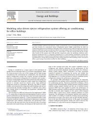
Figure 1-2 shows portions of a Mollier diagram developed by prediction methods 

described in later chapters. The dashed curves and points are obtained from estimates 

of liquid and vapor heat capacities, critical properties, vapor pressure, en- 

FIGURE 1-2 Mollier diagram for dichlorodifluoromethane. 

The solid lines represent measured data. 

Dashed lines and points represent results obtained by estimation 

methods when only the chemical formula and 

the normal boiling temperature are known. 






thalpy of vaporization, and pressure corrections to ideal-gas enthalpies and entropies. 

The substance is, of course, a well-known refrigerant, and its known properties 

are shown by the solid curves. While environmental concerns no longer permit use 

of CCl 2 F 2 , it nevertheless serves as a good example of building a full description 

from very little information. 

For a standard refrigeration cycle operating between 48.9 and 6.7C, the evaporator 

and condenser pressures are estimated to be 2.4 and 12.4 bar, vs. the known 

values 2.4 and 11.9 bar. The estimate of the heat absorption in the evaporator checks 

closely, and the estimated volumetric vapor rate to the compressor also shows good 

agreement: 2.39 versus 2.45 m 3 /hr per kW of refrigeration. (This number indicates 

the size of the compressor.) Constant-entropy lines are not shown in Fig. 1-2, but 

it is found that the constant-entropy line through the point for the low-pressure 

vapor essentially coincides with the saturated vapor curve. The estimated coefficient 

of performance (ratio of refrigeration rate to isentropic compression power) is estimated 

to be 3.8; the value obtained from the data is 3.5. This is not a very good 

check, but it is nevertheless remarkable because the only data used for the estimate 

were the normal boiling point and the chemical formula. 

Most estimation methods require parameters that are characteristic of single pure 

components or of constituents of a mixture of interest. The more important of these 

are considered in Chap. 2. 

The thermodynamic properties of ideal gases, such as enthalpies and Gibbs energies 

of formation and heat capacities, are covered in Chap. 3. Chapter 4 describes 

the PVT properties of pure fluids with the corresponding-states principle, equations 

of state, and methods restricted to liquids. Chapter 5 extends the methods of Chap. 

4 to mixtures with the introduction of mixing and combining rules as well as the 

special effects of interactions between different components. Chapter 6 covers other 

thermodynamic properties such as enthalpy, entropy, free energies and heat capacities 

of real fluids from equations of state and correlations for liquids. It also introduces 

partial properties and discusses the estimation of true vapor-liquid critical 

points. 

Chapter 7 discusses vapor pressures and enthalpies of vaporization of pure substances. 

Chapter 8 presents techniques for estimation and correlation of phase equilibria 

in mixtures. Chapters 9 to 11 describe estimation methods for viscosity, thermal 

conductivity, and diffusion coefficients. Surface tension is considered briefly in 

Chap. 12. 

The literature searched was voluminous, and the lists of references following 

each chapter represent but a fraction of the material examined. Of the many estimation 

methods available, in most cases only a few were selected for detailed 

discussion. These were selected on the basis of their generality, accuracy, and availability 

of required input data. Tests of all methods were often more extensive than 

those suggested by the abbreviated tables comparing experimental with estimated 

values. However, no comparison is adequate to indicate expected errors for new 

compounds. The average errors given in the comparison tables represent but a crude 

overall evaluation; the inapplicability of a method for a few compounds may so 

increase the average error as to distort judgment of the method’s merit, although 

efforts have been made to minimize such distortion. 

Many estimation methods are of such complexity that a computer is required. 

This is less of a handicap than it once was, since computers and efficient computer 

programs have become widely available. Electronic desk computers, which have 

become so popular in recent years, have made the more complex correlations practical. 

However, accuracy is not necessarily enhanced by greater complexity. 

The scope of the book is inevitably limited. The properties discussed were selected 

arbitrarily because they are believed to be of wide interest, especially to 






chemical engineers. Electrical properties are not included, nor are the properties of 

salts, metals, or alloys or chemical properties other than some thermodynamically 

derived properties such as enthalpy and the Gibbs energy of formation. 

This book is intended to provide estimation methods for a limited number of 

physical properties of fluids. Hopefully, the need for such estimates, and for a book 

of this kind, may diminish as more experimental values become available and as 

the continually developing molecular theory advances beyond its present incomplete 

state. In the meantime, estimation methods are essential for most process-design 

calculations and for many other purposes in engineering and applied science. 

REFERENCES 

Dewan, A. K., and M. A. Moore: ‘‘Physical Property Data Resources for the Practicing 

Engineer/Scientist in Today’s Information Age,’’ Paper 89C, AIChE 1999 Spring National 

Mtg., Houston, TX, March, 1999. Copyright Equilon Enterprise LLC. 

Din, F., (ed.): Thermodynamic Functions of Gases, Vol. 3, Butterworth, London, 1961. 

Maxwell, James Clerk: ‘‘Atoms,’’ Encyclopaedia Britannica, 9th ed., A. & C. Black, Edinburgh, 

1875–1888. 

Slater, J. C.: Modern Physics, McGraw-Hill, New York, 1955. 









CHAPTER TWO 

PURE COMPONENT 

CONSTANTS 

2-1 SCOPE 

Though chemical engineers normally deal with mixtures, pure component properties 

underlie much of the observed behavior. For example, property models intended 

for the whole range of composition must give pure component properties at the 

pure component limits. In addition, pure component property constants are often 

used as the basis for models such as corresponding states correlations for PVT 

equations of state (Chap. 4). They are often used in composition-dependent mixing 

rules for the parameters to describe mixtures (Chap. 5). 

As a result, we first study methods for obtaining pure component constants of 

the more commonly used properties and show how they can be estimated if no 

experimental data are available. These include the vapor-liquid critical properties, 

atmospheric boiling and freezing temperatures and dipole moments. Others such as 

the liquid molar volume and heat capacities are discussed in later chapters. Values 

for these properties for many substances are tabulated in Appendix A; we compare 

as many of them as possible to the results from estimation methods. Though the 

origins of current group contribution methods are over 50 years old, previous editions 

show that the number of techniques were limited until recently when computational 

capability allowed more methods to appear. We examine most of the 

current techniques and refer readers to earlier editions for the older methods. 

In Secs. 2-2 (critical properties), 2-3 (acentric factor) and 2-4 (melting and boiling 

points), we illustrate several methods and compare each with the data tabulated 

in Appendix A and with each other. All of the calculations have been done with 

spreadsheets to maximize accuracy and consistency among the methods. It was 

found that setting up the template and comparing calculations with as many substances 

as possible in Appendix A demonstrated the level of complexity of the 

methods. Finally, because many of the methods are for multiple properties and 

recent developments are using alternative approaches to traditional group contributions, 

Sec. 2-5 is a general discussion about choosing the best approach for pure 

component constants. Finally, dipole moments are treated in Sec. 2-6. 

Most of the estimation methods presented in this chapter are of the group, bond, 

or atom contribution type. That is, the properties of a molecule are usually established 

from contributions from its elements. The conceptual basis is that the intermolecular 

forces that determine the constants of interest depend mostly on the 

bonds between the atoms of the molecules. The elemental contributions are prin- 

2.1 




PURE COMPONENT CONSTANTS 

2.2 CHAPTER TWO 

cipally determined by the nature of the atoms involved (atom contributions), the 

bonds between pairs of atoms (bond contributions or equivalently group interaction 

contributions), or the bonds within and among small groups of atoms (group contributions). 

They all assume that the elements can be treated independently of their 

arrangements or their neighbors. If this is not accurate enough, corrections for 

specific multigroup, conformational or resonance effects can be included. Thus, 

there can be levels of contributions. The identity of the elements to be considered 

(group, bond, oratom) are normally assumed in advance and their contributions 

obtained by fitting to data. Usually applications to wide varieties of species start 

with saturated hydrocarbons and grow by sequentially adding different types of 

bonds, rings, heteroatoms and resonance. The formulations for pure component 

constants are quite similar to those of the ideal gas formation properties and heat 

capacities of Chap. 3; several of the group formulations described in Appendix C 

have been applied to both types of properties. 

Alternatives to group/bond/atom contribution methods have recently appeared. 

Most are based on adding weighted contributions of measured properties such as 

molecular weight and normal boiling point, etc. (factor analysis) or from ‘‘quantitative 

structure-property relationships’’ (QSPR) based on contributions from molecular 

properties such as electron or local charge densities, molecular surface area, 

etc. (molecular descriptors). Grigoras (1990), Horvath (1992), Katritzky, et al. 

(1995; 1999), Jurs [Egolf, et al., 1994], Turner, et al. (1998), and St. Cholakov, et 

al. (1999) all describe the concepts and procedures. The descriptor values are computed 

from molecular mechanics or quantum mechanical descriptions of the substance 

of interest and then property values are calculated as a sum of contributions 

from the descriptors. The significant descriptors and their weighting factors are 

found by sophisticated regression techniques. This means, however, that there are 

no tabulations of molecular descriptor properties for substances. Rather, a molecular 

structure is posed, the descriptors for it are computed and these are combined in 

the correlation. We have not been able to do any computations for these methods 

ourselves. However, in addition to quoting the results from the literature, since some 

tabulate their estimated pure component constants, we compare them with the values 

in Appendix A. 

The methods given here are not suitable for pseudocomponent properties such 

as for the poorly characterized mixtures often encountered with petroleum, coal and 

natural products. These are usually based on measured properties such as average 

molecular weight, boiling point, and the specific gravity (at 20C) rather than molecular 

structure. We do not treat such systems here, but the reader is referred to 

the work of Tsonopoulos, et al. (1986), Twu (1984, Twu and Coon, 1996), and 

Jianzhong, et al. (1998) for example. Older methods include those of Lin and Chao 

(1984) and Brule, et al. (1982), Riazi and Daubert (1980) and Wilson, et al. (1981). 

2-2 VAPOR-LIQUID CRITICAL PROPERTIES 

Vapor-liquid critical temperature, T c , pressure, P c , and volume, V c , are the purecomponent 

constants of greatest interest. They are used in many corresponding 

states correlations for volumetric (Chap. 4), thermodynamic (Chaps. 5–8), and 

transport (Chaps. 9 to 11) properties of gases and liquids. Experimental determination 

of their values can be challenging [Ambrose and Young, 1995], especially 

for larger components that can chemically degrade at their very high critical tem- 





PURE COMPONENT CONSTANTS 2.3 

peratures [Teja and Anselme, 1990]. Appendix A contains a data base of properties 

for all the substances for which there is an evaluated critical temperature tabulated 

by the Thermodynamics Research Center at Texas A&M University [TRC, 1999] 

plus some evaluated values by Ambrose and colleagues and by Steele and colleagues 

under the sponsorship of the Design Institute for Physical Properties Research 

(DIPPR) of the American Institute of Chemical Engineers (AIChE) in New 

York and NIST (see Appendix A for references). There are fewer evaluated P c and 

V c than T c . We use only evaluated results to compare with the various estimation 

methods. 

Estimation Techniques 

One of the first successful group contribution methods to estimate critical properties 

was developed by Lydersen (1955). Since that time, more experimental values have 

been reported and efficient statistical techniques have been developed that allow 

determination of alternative group contributions and optimized parameters. We examine 

in detail the methods of Joback (1984; 1987), Constantinou and Gani (1994), 

Wilson and Jasperson (1996), and Marrero and Pardillo (1999). After each is described 

and its accuracy discussed, comparisons are made among the methods, 

including descriptor approaches, and recommendations are made. Earlier methods 

such as those of Lyderson (1955), Ambrose (1978; 1979; 1980), and Fedors (1982) 

are described in previous editions; they do not appear to be as accurate as those 

evaluated here. 

Method of Joback. Joback (1984; 1987) reevaluated Lydersen’s group contribution 

scheme, added several new functional groups, and determined new contribution 

values. His relations for the critical properties are 

 

 

 

2 1 

T (K) T 0.584 0.965 N (tck) N (tck) (2-2.1) 

c b 

k 

k k 

k 

 

2 

P c (bar) 0.113 0.0032Natoms N k(pck) (2-2.2) 

k 

3 1 

V c (cm mol ) 17.5 N k(vck) (2-2.3) 

k 

where the contributions are indicated as tck, pck and vck. The group identities and 

Joback’s values for contributions to the critical properties are in Table C-1. For T c , 

a value of the normal boiling point, T b , is needed. This may be from experiment 

or by estimation from methods given in Sec. 2-4; we compare the results for both. 

An example of the use of Joback’s groups is Example 2-1; previous editions give 

other examples, as do Devotta and Pendyala (1992). 

Example 2-1 Estimate T c , P c , and V c for 2-ethylphenol by using Joback’s group 

method. 

solution 2-ethylphenol contains one —CH 3 , one —CH 2 —, four CH(ds), one 

ACOH (phenol) and two C(ds). Note that the group ACOH is only for the OH and 

does not include the aromatic carbon. From Appendix Table C-1 

 

 






Group k N k N k (tck) N k (pck) N k (vck) 

—CH 3 1 0.0141 0.0012 65 

—CH 2 — 1 0.0189 0 56 

CH(ds) 

4 0.0328 0.0044 164 

C(ds) 

2 0.0286 0.0016 64 

—ACOH (phenol) 1 0.0240 0.0184 25 

5 

k1 

0.1184 0.0232 324 

N k F k 

The value of N atoms 19, while T b 477.67 K. The Joback estimation method (Sec. 

2-4) gives T b 489.74 K. 

T T [0.584 0.965(0.1184) (0.1184) ] 

c 

b 

2 1 

698.1 K (with exp. T b), 715.7 K (with est. T b) 

P [0.113 0.0032(19) 0.0232] 

c 

2 

44.09 bar 

3 1 

Vc 

17.5 324 341.5 cm mol 

Appendix A values for the critical temperature and pressure are 703 K and 43.00 

bar. An experimental V c is not available. Thus the differences are 

Tc 

Difference (Exp. T b) 703 698.1 4.9 K or 0.7% 

Tc 

Difference (Est. T b) 703 715.7 12.7 K or 1.8% 

P Difference 43.00 44.09 1.09 bar or 2.5%. 

c 

A summary of the comparisons between estimations from the Joback method 

and experimental Appendix A values for T c , P c , and V c is shown in Table 2-1. The 

results indicate that the Joback method for critical properties is quite reliable for 

T c of all substances regardless of size if the experimental T b is used. When estimated 

values of T b are used, there is a significant increase in error, though it is less for 

compounds with 3 or more carbons (2.4% average increase for entries indicated by 

b 

in the table, compared to 3.8% for the whole database indicated by a ). 

For P c , the reliability is less, especially for smaller substances (note the difference 

between the a and b entries). The largest errors are for the largest molecules, 

especially fluorinated species, some ring compounds, and organic acids. Estimates 

can be either too high or too low; there is no obvious pattern to the errors. For V c , 

the average error is several percent; for larger substances the estimated values are 

usually too small while estimated values for halogenated substances are often too 

large. There are no obvious simple improvements to the method. Abildskov (1994) 

did a limited examination of Joback predictions (less than 100 substances) and 

found similar absolute percent errors to those of Table 2-1. 

A discussion comparing the Joback technique with other methods for critical 

properties is presented below and a more general discussion of group contribution 

methods is in Sec. 2-5. 

Method of Constantinou and Gani (CG). Constantinou and Gani (1994) developed 

an advanced group contribution method based on the UNIFAC groups (see 

Chap. 8) but they allow for more sophisticated functions of the desired properties 






TABLE 2-1 

Summary of Comparisons of Joback Method with Appendix A Database 

Property # Substances AAE c A%E c # Err 10% d # Err 5% e 

T c (Exp. T b ) ƒ , K 352 a 6.65 1.15 0 345 

289 b 6.68 1.10 0 286 

T c (Est. T b ) g , K 352 a 25.01 4.97 46 248 

290 b 20.19 3.49 18 229 

P c , bar 328 a 2.19 5.94 59 196 

266 b 1.39 4.59 30 180 

V c ,cm 3 mol 1 236 a 12.53 3.37 13 189 

185 b 13.98 3.11 9 148 

a 

The number of substances in Appendix A with data that could be tested with the method. 

b 

The number of substances in Appendix A having 3 or more carbon atoms with data that could be 

tested with the method. 

c 

AAE is average absolute error in the property; A%E is average absolute percent error. 

d 

The number of substances for which the absolute percent error was greater than 10%. 

e 

The number of substances for which the absolute percent error was less than 5%. The number of 

substances with errors between 5% and 10% can be determined from the table information. 

ƒ 

The experimental value of T b in Appendix A was used. 

g 

The value of T b used was estimated by Joback’s method (see Sec. 2-4). 

and also for contributions at a ‘‘Second Order’’ level. The functions give more 

flexibility to the correlation while the Second Order partially overcomes the limitation 

of UNIFAC which cannot distinguish special configurations such as isomers, 

multiple groups located close together, resonance structures, etc., at the ‘‘First Order.’’ 

The general CG formulation of a function ƒ[F] of a property F is 

 

 

 

F ƒ N (F ) W M(F ) (2-2.4) 

k 

k 1k j 2j 

j 

where ƒ can be a linear or nonlinear function (see Eqs. 2-2.5 to 2-2.7), N k is the 

number of First-Order groups of type k in the molecule; F 1k is the contribution for 

the First-Order group labeled 1k to the specified property, F; M j is the number of 

Second-Order groups of type j in the molecule; and F 2j is the contribution for the 

Second-Order group labeled 2j to the specified property, F. The value of W is set 

to zero for First-Order calculations and set to unity for Second-order calculations. 

For the critical properties, the CG formulations are 

 

 

T (K) 181.128 ln N (tc1k) W M(tc2j ) (2-2.5) 

 

c k j 

k 

j 

 

 

 

P (bar) N (pc1k) W M(pc2j ) 0.10022 1.3705 (2-2.6) 

c k j 

k 

j 

 

 

3 1 

V c(cm mol ) 0.00435 N k(vc1k) W M(vc2j j ) (2-2.7) 

k 

j 

Note that T c does not require a value for T b . The group values for Eqs. (2-2.5) to 

(2-2.7) are given in Appendix Tables C-2 and C-3 with sample assignments shown 

in Table C-4. 

 

 

2 

 

 

 






Example 2-2 Estimate T c , P c , and V c for 2-ethylphenol by using Constantinou and 

Gani’s group method. 

solution The First-Order groups for 2-ethylphenol are one CH 3 , four ACH, one 

ACCH2, and one ACOH. There are no Second-Order groups (even though the ortho 

proximity effect might suggest it) so the First Order and Second Order calculations are 

the same. From Appendix Tables C-2 and C-3 

Group k N k N k (tc1k) N k (pc1k) N k (vc1k) 

CH 3 1 1.6781 0.019904 0.07504 

ACH 4 14.9348 0.030168 0.16860 

ACCH2 1 10.3239 0.012200 0.10099 

ACOH 1 25.9145 0.007444 0.03162 

5 

NF 

k k 

k1 

52.8513 0.054828 0.37625 

T 181.128 ln[52.8513 W(0)] 718.6 K 

c 

P [0.054828 W(0) 0.10022] 

c 

2 

1.3705 42.97 bar 

3 1 

Vc 

(0.00435 [0.37625 W(0)])1000 371.9 cm mol 

The Appendix A values for the critical temperature and pressure are 703.0 K and 43.0 


T 

c 

Difference 703.0 718.6 15.6 K or 2.2% 

1 

Pc 

Difference 43.0 42.97 0.03 kJ mol or 0.1%. 

Example 2-3 Estimate T c , P c , and V c for the four butanols using Constantinou and 

Gani’s group method 

solution 

The First- and Second-Order groups for the butanols are: 

Groups/Butanol 

1-butanol 

2-methyl- 

1-propanol 

2-methyl- 

2-propanol 

2-butanol 

# First-Order groups, N k — — — — 

CH 3 1 2 3 2 

CH 2 3 1 0 1 

CH 0 1 0 1 

C 0 0 1 0 

OH 1 1 1 1 

Second-Order groups, M j — — — — 

(CH 3 ) 2 CH 0 1 0 0 

(CH 3 ) 3 C 0 0 1 0 

CHOH 0 1 0 1 

COH 0 0 1 0 

Since 1-butanol has no Second-Order group, its calculated results are the same for both 

orders. Using values of group contributions from Appendix Tables C-2 and C-3 and 

experimental values from Appendix A, the results are: 






Property/Butanol 

1-butanol 

2-methyl- 

1-propanol 

2-methyl- 

2-propanol 

2-butanol 

T c ,K 

Experimental 563.05 547.78 506.21 536.05 

Calculated (First Order) 558.91 548.06 539.37 548.06 

Abs. percent Err. (First Order) 0.74 0.05 6.55 2.24 

Calculated (Second Order) 558.91 543.31 497.46 521.57 

Abs. percent Err. (Second Order) 0.74 0.82 1.73 2.70 

P c , bar 

Experimental 44.23 43.00 39.73 41.79 





V c ,cm 3 mol 1 

Experimental 275.0 273.0 275.0 269.0 





The First Order results are generally good except for 2-methyl-2-propanol (tbutanol). 

The steric effects of its crowded methyl groups make its experimental value 

quite different from the others; most of this is taken into account by the First-Order 

groups, but the Second Order contribution is significant. Notice that the Second Order 

contributions for the other species are small and may change the results in the wrong 

direction so that the Second Order estimate can be slightly worse than the First Order 

estimate. This problem occurs often, but its effect is normally small; including Second 

Order effects usually helps and rarely hurts much. 

A summary of the comparisons between estimations from the Constantinou and 

Gani method and experimental values from Appendix A for T c , P c , and V c is shown 

in Table 2-2. 

The information in Table 2-2 indicates that the Constantinou/Gani method can 

be quite reliable for all critical properties, though there can be significant errors for 

some smaller substances as indicated by the lower errors in Table 2-2B compared 

to Table 2-2A for T c and P c but not for V c . This occurs because group additivity is 

not so accurate for small molecules even though it may be possible to form them 

from available groups. In general, the largest errors of the CG method are for the 

very smallest and for the very largest molecules, especially fluorinated and larger 

ring compounds. Estimates can be either too high or too low; there is no obvious 

pattern to the errors. 

Constantinou and Gani’s original article (1994) described tests for 250 to 300 

substances. Their average absolute errors were significantly less than those of Table 

2-2. For example, for T c they report an average absolute error of 9.8 K for First 

Order and 4.8 K for Second Order estimations compared to 18.5K and 17.7 K here 

for 335 compounds. Differences for P c and V c were also much less than given here. 

Abildskov (1994) made a limited study of the Constantinou/Gani method (less than 

100 substances) and found absolute and percent errors very similar to those of Table 

2-2. Such differences typically arise from different selections of the substances and 

data base values. In most cases, including Second Order contributions improved the 






TABLE 2-2 Summary of Constantinou/Gani Method 

Compared to Appendix A Data Base 

A. All substances in Appendix A with data that could be 

tested with the method 

Property T c ,K P c , bar V c ,cm 3 mol 1 

# Substances (1st) a 335 316 220 

AAE (1st) b 18.48 2.88 15.99 

A%E (1st) b 3.74 7.37 4.38 

# Err 10% (1st) c 28 52 18 

# Err 5% (1st) d 273 182 160 

# Substances (2nd) e 108 99 76 

AAE (2nd) b 17.69 2.88 16.68 

A%E (2nd) b 13.61 7.33 4.57 

# Err 10% (2nd) c 29 56 22 

# Err 5% (2nd) d 274 187 159 

# Better (2nd) ƒ 70 58 35 

Ave. % 1st to 2nd g 0.1 0.2 0.4 

B. All substances in Appendix A having 3 or more carbon 

atoms with data that could be tested with the method 

Property T c ,K P c , bar V c ,cm 3 mol 1 

# Substances (1st) a 286 263 180 

AAE (1st) b 13.34 1.8 16.5 

A%E (1st) b 2.25 5.50 3.49 

# Err 10% (1st) c 4 32 10 

# Err 5% (1st) d 254 156 136 

# Substances (2nd) e 104 96 72 

AAE (2nd) b 12.49 1.8 17.4 

A%E (2nd) b 2.12 5.50 3.70 

# Err 10% (2nd) c 6 36 15 

# Err 5% (2nd) d 254 160 134 

# Better (2nd) ƒ 67 57 32 

Ave. % 1st to 2nd g 0.3 0.1 0.5 

a 

The number of substances in Appendix A with data that could be 


b 

AAE is average absolute error in the property; A%E is average 

absolute percent error. 

c 

The number of substances for which the absolute percent error was 

greater than 10%. 

d 


less than 5%. The number of substances with errors between 5% and 

10% can be determined from the table information. 

e 

The number of substances for which Second-Order groups are defined 

for the property. 

f 

The number of substances for which the Second Order result is more 

accurate than First Order. 

g 

The average improvement of Second Order compared to First Order. 

A negative value indicates that overall the Second Order was less accurate. 






results 1 to 3 times as often as it degraded them, but except for ring compounds 

and olefins, the changes were rarely more than 1 to 2%. Thus, Second Order contributions 

make marginal improvements overall and it may be worthwhile to include 

the extra complexity only for some individual substances. In practice, examining 

the magnitude of the Second Order values for the groups involved should provide 

a user with the basis for including them or not. 

A discussion comparing the Constantinou/Gani technique with other methods 

for critical properties is presented below and a more general discussion is found in 

Sec. 2-5. 

Method of Wilson and Jasperson. Wilson and Jasperson (1996) reported three 

methods for T c and P c that apply to both organic and inorganic species. The Zero- 

Order method uses factor analysis with boiling point, liquid density and molecular 

weight as the descriptors. At the First Order, the method uses atomic contributions 

along with boiling point and number of rings, while the Second Order method also 

includes group contributions. The Zero-Order has not been tested here; it is iterative 

and the authors report that it is less accurate by as much as a factor of two or three 

than the others, especially for P c . The First Order and Second Order methods use 

the following equations: 

 

 

T T 0.048271 0.019846N N (tck) M (tcj) (2-2.8) 

c b r k j 

k 

j 

 

P 0.0186233T /[0.96601 exp(Y)] 

c 

c 

Y 0.00922295 0.0290403N 0.041 N (pck) M (pcj ) 

 

 

 

r k j 

k 

j 

 

0.2 

(2-2.9a) 

 

(2-2.9b) 

where N r is the number of rings in the compound, N k is the number of atoms of 

type k with First Order atomic contributions tck and pck while M j is the number 

of groups of type j with Second-Order group contributions tcj and pcj. Values 

of the contributions are given in Table 2-3 both for the First Order Atomic Contributions 

and for the Second-Order Group Contributions. Note that T c requires T b . 

Application of the Wilson and Jasperson method is shown in Example 2-4. 

Example 2-4 

method. 

Estimate T c and P c for 2-ethylphenol by using Wilson and Jasperson’s 

solution The atoms of 2-ethylphenol are 8 C, 10 H, 1 O and there is 1 ring. 

For groups, there is 1 OH for ‘‘C5 or more.’’ The value of T b from Appendix A is 

477.67 K; the value estimated by the Second Order method of Constantinou and Gani 

(Eq. 2-4.4) is 489.24 K. From Table 2-3A 

Atom k N k N k (tck) N k (pck) 

C 8 0.06826 5.83864 

H 10 0.02793 1.26600 

O 1 0.02034 0.43360 

3 

NF k k 

k1 

— 0.11653 7.53824 






TABLE 2-3A Wilson-Jasperson (1996) 

Atomic Contributions for Eqs. (2-2.8) and 

(2-2.9) 

Atom tck pck 

H 0.002793 0.12660 

D 0.002793 0.12660 

T 0.002793 0.12660 

He 0.320000 0.43400 

B 0.019000 0.91000 

C 0.008532 0.72983 

N 0.019181 0.44805 

O 0.020341 0.43360 

F 0.008810 0.32868 

Ne 0.036400 0.12600 

Al 0.088000 6.05000 

Si 0.020000 1.34000 

P 0.012000 1.22000 

S 0.007271 1.04713 

Cl 0.011151 0.97711 

Ar 0.016800 0.79600 

Ti 0.014000 1.19000 

V 0.018600 ***** 

Ga 0.059000 ***** 

Ge 0.031000 1.42000 

As 0.007000 2.68000 

Se 0.010300 1.20000 

Br 0.012447 0.97151 

Kr 0.013300 1.11000 

Rb 0.027000 ***** 

Zr 0.175000 1.11000 

Nb 0.017600 2.71000 

Mo 0.007000 1.69000 

Sn 0.020000 1.95000 

Sb 0.010000 ***** 

Te 0.000000 0.43000 

I 0.005900 1.315930 

Xe 0.017000 1.66000 

Cs 0.027500 6.33000 

Hf 0.219000 1.07000 

Ta 0.013000 ***** 

W 0.011000 1.08000 

Re 0.014000 ***** 

Os 0.050000 ***** 

Hg 0.000000 0.08000 

Bi 0.000000 0.69000 

Rn 0.007000 2.05000 

U 0.015000 2.04000 






TABLE 2-3B Wilson-Jasperson (1996) Group 

Contributions for Eqs. (2-2.8) and (2-2.9) 

Group tcj pcj 

—OH, C 4 or less 0.0350 0.00 

—OH, C 5 or more 0.0100 0.00 

—O— 0.0075 0.00 

—NH 2 , NH, N— 0.0040 0.00 

—CHO 0.0000 0.50 

CO 0.0550 0.00 

—COOH 0.0170 0.50 

—COO— 0.0150 0.00 

—CN 0.0170 1.50 

—NO 2 0.0200 1.00 

Organic Halides (once/molecule) 0.0020 0.00 

—SH, —S—, —SS— 0.0000 0.00 

Siloxane bond 0.0250 0.50 

Thus the First Order estimates are 

T 477.67/[0.048271 0.019846 0.11653] 

c 

0.2 

702.9 K 

P 0.0186233(704.1)/[0.96601 exp(Y)] 37.94 bar 

c 

Y 0.0092229 0.0290403 0.3090678 0.2708046 

From Table 2-3B there is the ‘‘OH, C5 or more’’ contribution of N k tck 0.01 

though for P c there is no contribution. Thus only the Second Order estimate for T c is 

changed to 

T 477.67/[0.048271 0.019846 0.11653 0.01] 

c 

0.2 

693.6 K 

If the estimated value of T b is used, the result is 710.9 K. The Appendix A values 

for the critical properties are 703.0 K and 43.0 bar, respectively. Thus the differences 

are 

First Order T c (Exp. T b) Difference 703.0 702.9 0.1 K or 0.0% 

T (Est. T ) 

c 

b 


P Difference 43.0 37.9 5.1 bar or 11.9%. 

c 

Second Order T c (Exp. T b) Difference 703.0 693.6 9.4 K or 1.3% 

T (Est. T ) 

c 

b 

Difference 703.0 710.9 7.9Kor1.1% 

P ( First Order) Difference 43.0 37.9 5.1 bar or 11.9%. 

c 

The First Order estimate for T c is more accurate than the Second Order estimate which 

occasionally occurs. 

A summary of the comparisons between estimations from the Wilson and Jasperson 

method and experimental values from Appendix A for T c and P c are shown 

in Table 2-4. Unlike the Joback and Constantinou/Gani method, there was no dis- 






TABLE 2-4 

Summary of Wilson/Jasperson Method Compared to Appendix A Data Base 

Property 

T c ,K 

(Exp. T b )* 

T c ,K 

(Est T b ) 

P c , bar 

(Exp T c )# 

P c , bar 

(Est T c )@ 

# Substances a 353 — 348 348 

AAE (First Order) b 8.34 — 2.08 2.28 

A%E (First Order) b 1.50 — 5.31 5.91 

# Err 10% (First Order) c 0 — 54 66 

# Err 5% (First Order) d 220 — 234 220 

# Substances e 180 289 23 23 

AAE (Second Order) b 6.88 16.71 1.82 2.04 

A%E (Second Order) b 1.22 2.95 4.74 5.39 

# Err 10% (Second Order) c 0 15 46 57 

# Err 5% (Second Order) d 348 249 245 226 

# Better (Second Order) ƒ 120 77 19 18 

Ave. % First to Second Order g 0.5 1.8 8.6 7.9 

* Eq. (2-2.8) with experimental T b . 

Eq. (2-2.8) with T b estimated from Second Order Method of Constantinou and Gani (1994). 

# Eq. (2-2.9) with experimental T c . 

@ Eq. (2-2.9) with T c estimated using Eq. (2-2.8) and experimental T b . 

a 


b 


c 


d 



e 

The number of substances for which Second-Order groups are defined for the property. 

ƒ 

The number of substances for which the Second Order result is more accurate than First Order. 

g 

The average improvement of Second Order compared to First Order. A negative value indicates that 

overall the Second Order was less accurate. 

cernible difference in errors between small and large molecules for either property 

so only the overall is given. 

The information in Table 2-4 indicates that the Wilson/Jasperson method is very 

accurate for both T c and P c . When present, the Second Order group contributions 

normally make significant improvements over estimates from the First Order atom 

contributions. The accuracy for P c deteriorates only slightly with an estimated value 

of T c if the experimental T b is used. The accuracy of T c is somewhat less when the 

required T b is estimated with the Second Order method of Constantinou and Gani 

(1994) (Eq. 2-4.4). Thus the method is remarkable in its accuracy even though it 

is the simplest of those considered here and applies to all sizes of substances 

equally. 

Wilson and Jasperson compared their method with results for 700 compounds 

of all kinds including 172 inorganic gases, liquids and solids, silanes and siloxanes. 

Their reported average percent errors for organic substance were close to those 

found here while they were somewhat larger for the nonorganics. The errors for 

organic acids and nitriles are about twice those for the rest of the substances. 

Nielsen (1998) studied the method and found similar results. 

Discussion comparing the Wilson/Jasperson technique with other methods for 

critical properties is presented below and a more general discussion is in Sec. 2-5. 

Method of Marrero and Pardillo. Marrero-Marejón and Pardillo-Fontdevila 

(1999) describe a method for T c , P c , and V c that they call a group interaction 

contribution technique or what is effectively a bond contribution method. They give 






equations that use values from pairs of atoms alone, such as C & —N, or 

with hydrogen attached, such as CH 3 — & —NH 2 . Their basic equations are 

2 

 

 

 

c b 

k 

k k 

k 

T T / 0.5851 0.9286 N tcbk Ntcbk (2-2.10) 

 

 

P 0.1285 0.0059N Npcbk (2-2.11) 

c atoms k 

k 

 

V 25.1 N vcbk (2-2.12) 

c 

k 

k 

where N atoms is the number of atoms in the compound, N k is the number of atoms 

of type k with contributions tcbk, pcbk, and vcbk. Note that T c requires T b ,but 

Marrero and Pardillo provide estimation methods for T b (Eq. 2-4.5). 

Values of contributions for the 167 pairs of groups (bonds) are given in Table 

2-5. These were obtained directly from Dr. Marrero and correct some misprints in 

the original article (1999). The notation of the table is such that when an atom is 

bonded to an element other than hydrogen, — means a single bond, or means 

2 single bonds, means a double bond and means a triple bond, [r] means 

that the group is in a ring such as in aromatics and naphthenics, and [rr] means the 

pair connects 2 rings as in biphenyl or terphenyl. Thus, the pair C &F— means 

that the C is bonded to 4 atoms/groups that are not hydrogen and one of the bonds 

is to F, while C &F— means that the C atom is doubly bonded to another 

atom and has 2 single bonds with 1 of the bonds being to F. Bonding by multiple 

bonds is denoted by both members of the pair having [ ] or []; if they both 

have a or a without the brackets [], they will also have at least 1 — and the 

bonding of the pair is via a single bond. Therefore, the substance CHFCFCF 3 

would have 1 pair of [ ]CH— &[ ]C, 1 pair of CH— &F—, 1 pair of 

C & —F, 1 pair of C and C, and 3 pairs of C & —F. The location 

of bonding in esters is distinguished by the use of [ ] as in pairs 20, 21, 67, 100 

and 101. For example, in the pair 20, the notation CH 3 — & —COO[—] means 

that CH 3 — is bonded to an O to form an ester group, CH 3 —O—CO—, whereas 

in the pair 21, the notation CH 3 — &[—]COO— means that CH 3 — is bonded to 

the C to form CH 3 —CO—O—. Of special note is the treatment of aromatic rings; 

it differs from other methods considered in this section because it places single and 

double bonds in the rings at specific locations, affecting the choice of contributions. 

This method of treating chemical structure is the same as used in traditional Handbooks 

of Chemistry such as Lange’s (1999). We illustrate the placement of side 

groups and bonds with 1-methylnaphthalene in Example 2-5. The locations of the 

double bonds for pairs 130, 131, and 139 must be those illustrated as are the single 

bonds for pairs 133, 134 and 141. The positions of side groups must also be carefully 

done; the methyl group with bond pair 10 must be placed at the ‘‘top’’ of the 

diagram since it must be connected to the 131 and 141 pairs. If the location of it 

or of the double bond were changed, the contributions would change. 

Example 2-5 List the pairs of groups (bonds) of the Marrero/Pardillo (1999) method 

for 1-methylnaphthalene. 

solution The molecular structure and pair numbers associated with the bonds from 

Table 2-5 are shown in the diagram. 

 

2 






TABLE 2-5 Marrero-Pardillo (1999) Contributions for Eqs. (2-2.10) to (2-2.12) and (2-4.5) 

Pair # Atom/Group Pairs tcbk pcbk vcbk tbbk 

1 CH 3 —&CH 3 — 0.0213 0.0618 123.2 113.12 

2 CH 3 —&—CH 2 — 0.0227 0.0430 88.6 194.25 

3 CH 3 —&CH— 0.0223 0.0376 78.4 194.27 

4 CH 3 —&C 0.0189 0.0354 69.8 186.41 

5 CH 3 — & CH— 

0.8526 0.0654 81.5 137.18 

6 CH 3 —& C 

0.1792 0.0851 57.7 182.20 

7 CH 3 —&C— 0.3818 0.2320 65.8 194.40 

8 CH 3 —&CH— [r] 0.0214 0.0396 58.3 176.16 

9 CH 3 —&C [r] 0.1117 0.0597 49.0 180.60 

10 CH 3 —& C [r] 

0.0987 0.0746 71.7 145.56 

11 CH 3 —&F— 0.0370 0.0345 88.1 160.83 

12 CH 3 — & Cl— 0.9141 0.0231 113.8 453.70 

13 CH 3 — & Br— 0.9166 0.0239 ***** 758.44 

14 CH 3 —&I— 0.9146 0.0241 ***** 1181.44 

15 CH 3 —&—OH 0.0876 0.0180 92.9 736.93 

16 CH 3 —&—O— 0.0205 0.0321 66.0 228.01 

17 CH 3 —&CO 0.0362 0.0363 88.9 445.61 

18 CH 3 — & —CHO 0.0606 0.0466 128.9 636.49 

19 CH 3 — & —COOH 0.0890 0.0499 145.9 1228.84 

20 CH 3 — & —COO[—] 0.0267 0.1462 93.3 456.92 

21 CH 3 — & [—]COO— 0.0974 0.2290 108.2 510.65 

22 CH 3 —&—NH 2 0.0397 0.0288 ***** 443.76 

23 CH 3 —&—NH— 0.0313 0.0317 ***** 293.86 

24 CH 3 —&N— 0.0199 0.0348 76.3 207.75 

25 CH 3 —&—CN 0.0766 0.0507 147.9 891.15 

26 CH 3 —&—NO 2 0.0591 0.0385 148.1 1148.58 

27 CH 3 —&—SH 0.9192 0.0244 119.7 588.31 

28 CH 3 —&—S— 0.0181 0.0305 87.9 409.85 

29 —CH 2 —&—CH 2 — 0.0206 0.0272 56.6 244.88 

30 —CH 2 —&CH— 0.0134 0.0219 40.2 244.14 

31 —CH 2 —&C 0.0098 0.0162 32.0 273.26 

32 —CH 2 — & CH— 

0.8636 0.0818 50.7 201.80 

33 —CH 2 —& C 

0.1874 0.1010 24.0 242.47 

34 —CH 2 —&C— 0.4160 0.2199 33.9 207.49 

35 —CH 2 —&CH— [r] 0.0149 0.0265 31.9 238.81 

36 —CH 2 —&C [r] 0.1193 0.0423 ***** 260.00 

37 —CH 2 —& C [r] 

0.1012 0.0626 52.1 167.85 

38 —CH 2 —&F— 0.0255 0.0161 49.3 166.59 

39 —CH 2 — & Cl— 0.0162 0.0150 80.8 517.62 

40 —CH 2 — & Br— 0.0205 0.0140 101.3 875.85 

41 —CH 2 —&I— 0.0210 0.0214 ***** 1262.80 

42 —CH 2 —&—OH 0.0786 0.0119 45.2 673.24 

43 —CH 2 —&—O— 0.0205 0.0184 34.5 243.37 

44 —CH 2 —&CO 0.0256 0.0204 62.3 451.27 

45 —CH 2 — & —CHO 0.0267 0.0210 106.1 648.70 

46 —CH 2 — & —COOH 0.0932 0.0253 114.0 1280.39 

47 —CH 2 — & —COO[—] 0.0276 0.1561 69.9 475.65 

48 —CH 2 — & [—]COO— 0.0993 0.2150 79.1 541.29 

49 —CH 2 —&—NH 2 0.0301 0.0214 63.3 452.30 

50 —CH 2 —&—NH— 0.0248 0.0203 49.4 314.71 







(Continued) 


51 —CH 2 —&N— 0.0161 0.0170 32.7 240.08 

52 —CH 2 —&—CN 0.0654 0.0329 113.5 869.18 

53 —CH 2 —&—SH 0.0137 0.0163 93.3 612.31 

54 —CH 2 —&—S— 0.0192 0.0173 57.9 451.03 

55 CH— & CH— 0.0039 0.0137 18.3 291.41 

56 CH— & C 0.0025 0.0085 8.6 344.06 

57 CH— & CH— 

0.8547 0.0816 48.9 179.96 

58 CH— & C 

0.1969 0.1080 4.3 249.10 

59 CH— & CH— [r] 0.0025 0.0168 ***** 295.33 

60 CH— & C [r] 

0.1187 0.0556 ***** 132.66 

61 CH— & F— 0.0200 0.0147 37.7 68.80 

62 CH— & Cl— 0.0142 0.0131 68.6 438.47 

63 CH— & —OH 0.0757 0.0093 45.6 585.99 

64 CH— & —O— 0.0162 0.0155 23.7 215.94 

65 CH— & CO 0.0194 0.0112 39.3 434.45 

66 CH— & —CHO 0.0406 0.0280 92.2 630.07 

67 CH— & [—]COO— 0.0918 0.2098 72.3 497.58 

68 CH— & —COOH 0.1054 0.0358 110.2 1270.16 

69 CH— & —NH 2 0.0286 0.0212 39.2 388.44 

70 CH— & —NH— 0.0158 0.0162 ***** 260.32 

71 C & C 0.0084 0.0002 22.7 411.56 

72 C & CH— 

0.8767 0.0953 23.4 286.30 

73 C & C 

0.2061 0.1109 8.8 286.42 

74 C & C [r] 0.0207 0.0213 ***** 456.90 

75 C & CH— [r] 0.0049 0.0111 ***** 340.00 

76 C & C [r] 

0.1249 0.0510 ***** 188.99 

77 C &F— 0.0176 0.0161 30.0 16.64 

78 C &Cl— 0.0133 0.0129 63.7 360.79 

79 C &Br— 0.0084 0.0121 85.7 610.26 

80 C &—OH 0.0780 0.0094 40.6 540.38 

81 C &—O— 0.0156 0.0103 40.8 267.26 

82 C & CO 0.0114 0.0085 62.1 373.71 

83 C & —COOH 0.1008 0.0455 89.0 1336.54 

84 [ ]CH 2 & [ ]CH 2 

0.9129 0.0476 105.3 51.13 

85 [ ]CH 2 & —CH[ ] 

0.8933 0.1378 77.4 205.73 

86 [ ]CH 2 & C[ ] 

0.4158 0.2709 99.2 245.27 

87 [ ]CH 2 & C[ ] 

0.0123 0.0239 68.4 183.55 

88 —CH[ ] & —CH[ ] 

1.7660 0.2291 47.8 334.64 

89 —CH[ ] & C[ ] 

1.2909 0.3613 73.6 354.41 

90 —CH[ ] & C[ ] 

0.8945 0.1202 43.6 316.46 

91 CH— & CH— 

1.7377 0.1944 42.1 174.18 

92 CH— & C 

1.0731 0.2146 16.6 228.38 

93 CH— & C— 

1.2865 0.1087 ***** 174.39 

94 CH— & C [r] 

0.9929 0.0533 ***** 184.20 

95 CH— & F— 

0.8623 0.0929 41.4 5.57 

96 CH— & Cl— 

0.8613 0.0919 68.7 370.60 

97 CH— & —O— 

0.8565 0.0947 36.4 204.81 

98 CH— & —CHO 

0.8246 0.0801 ***** 658.53 

99 CH— & —COOH 

0.7862 0.0806 107.4 1245.86 

100 CH— & —COO[—] 

0.8818 0.2743 55.2 423.86 







(Continued) 


101 CH— & [—]COO— 

0.7780 0.1007 64.1 525.35 

102 CH— & —CN 

0.8122 0.0771 107.4 761.36 

103 C[ ] & C[ ] 

0.8155 0.4920 93.7 399.58 

104 C[ ] & C[ ] 

0.4009 0.2502 58.1 321.02 

105 C & C [r] 

0.3043 0.0705 ***** 250.88 

106 C &F— 

0.1868 0.1064 14.6 37.99 

107 C &Cl— 

0.1886 0.1102 43.3 367.05 

108 C[ ] & O[ ] 

0.0159 0.0010 51.4 160.42 

109 CH[] & CH[] 0.0288 0.0226 87.6 120.85 

110 CH[] &—C[] 0.4222 0.1860 73.1 222.40 

111 —C[] &—C[] 0.7958 0.3933 64.3 333.26 

112 —CH 2 — [r] & —CH 2 — [r] 0.0098 0.0221 47.2 201.89 

113 —CH 2 — [r] & CH— [r] 0.0093 0.0181 47.5 209.40 

114 —CH 2 — [r] & C [r] 0.1386 0.0081 49.9 182.74 

115 —CH 2 — [r] & CH— [r] 0.0976 0.1034 42.5 218.07 

116 —CH 2 — [r] & C [r] 0.1089 0.0527 ***** 106.21 

117 —CH 2 — [r] & —O— [r] 0.0092 0.0119 29.2 225.52 

118 —CH 2 — [r] & CO [r] 0.0148 0.0177 50.7 451.74 

119 —CH 2 — [r] & —NH— [r] 0.0139 0.0127 38.8 283.55 

120 —CH 2 — [r] & —S— [r] 0.0071 ***** ***** 424.13 

121 CH— [r] & CH— [r] 0.0055 0.0088 33.9 210.66 

122 CH— [r] & C [r] 0.1341 0.0162 ***** 220.24 

123 CH— [r] & CH— [rr] ***** ***** ***** 254.50 

124 CH— [r] & C[ ] [rr] ***** ***** ***** 184.36 

125 CH— [r] & —O— [r] 0.0218 0.0091 19.2 169.17 

126 CH— [r] & —OH 0.0737 0.0220 597.82 

127 C [r] & C [r] 0.0329 0.0071 36.2 348.23 

128 C [r] & C [r] 

***** ***** ***** 111.51 

129 C [r] & F— 0.0314 0.0119 18.4 41.35 

130 —CH[ ] [r] & —CH[ ] [r] 0.2246 0.1542 36.5 112.00 

131 —CH[ ] [r] & C[ ] [r] 0.3586 0.1490 34.4 291.15 

132 —CH[ ] [r] & —N[ ] [r] 0.3913 0.1356 8.3 221.55 

133 CH— [r] & CH— [r] 0.2089 0.1822 39.3 285.07 

134 CH— [r] & C [r] 

0.2190 0.1324 29.8 237.22 

135 CH— [r] & —O— [r] 0.1000 0.0900 40.3 171.59 

136 CH— [r] & —NH— [r] 0.0947 ***** ***** 420.54 

137 CH— [r] & N— [r] 0.4067 0.1491 65.9 321.44 

138 CH— [r] & —S— [r] 0.1027 0.0916 40.8 348.00 

139 C[ ] [r] & C[ ] [r] 0.4848 0.1432 37.8 477.77 

140 C[ ] [r] & —N[ ] [r] 0.2541 ***** ***** 334.09 

141 C [r] & C [r] 

0.2318 0.0809 20.6 180.07 

142 C [r] & C [rr] 

0.2424 0.0792 51.7 123.05 

143 C [r] & —O— [r] 

0.1104 0.0374 0.3 134.23 

144 C [r] & N— [r] 

0.3972 0.0971 35.6 174.31 

145 C [r] & F— 

0.1069 0.0504 23.7 48.79 

146 C [r] & Cl— 

0.1028 0.0512 60.3 347.33 

147 C [r] & Br— 

0.1060 0.0548 83.2 716.23 

148 C [r] & I— 

0.1075 0.0514 110.2 1294.98 

149 C [r] & —OH 

0.0931 0.0388 8.5 456.25 

150 C [r] & —O— 

0.0997 0.0523 ***** 199.70 







(Continued) 


151 C [r] & CO 

0.1112 0.0528 46.3 437.51 

152 C [r] & —CHO 

0.0919 0.0597 ***** 700.06 

153 C [r] & —COOH 

0.0313 0.0684 100.2 1232.55 

154 C [r] & [—]COO— 

0.0241 0.2573 55.2 437.78 

155 C [r] & —NH 2 

0.0830 0.0579 33.2 517.75 

156 C [r] & —NH— 

0.0978 0.0471 ***** 411.29 

157 C [r] & N— 

0.0938 0.0462 ***** 422.51 

158 C [r] & —CN 

0.0768 0.0625 ***** 682.19 

159 Cl— & CO 0.0191 0.0125 84.0 532.24 

160 [—]COO— & [—]COO— 0.1926 0.0878 ***** 1012.51 

161 —O— [r] & N— [r] 0.5728 ***** ***** 382.25 

162 CO & —O— 0.3553 0.0176 ***** 385.36 

163 —H & —CHO 0.0422 0.0123 ***** 387.17 

164 —H & —COOH 0.0690 ***** ***** 1022.45 

165 —H & [—]COO— 0.0781 0.1878 51.2 298.12 

166 —NH— & —NH 2 0.0301 ***** ***** 673.59 

167 —S— & —S— 0.0124 ***** ***** 597.59 

Pair # 

Atom/Group Pair 

N k 

141 

10 CH 3 

131 H 130 

H 

133 

139 H 

134 133 

H H 

130 H134H 

130 

10 

130 

131 

133 

134 

139 

141 

CH3— & C [r] 

—CH[ ] [r] & —CH[ ] [r] 

—CH[ ] [r] & C[ ] [r] 

CH— [r] & CH— [r] 

CH— [r] & C [r] 

C[ ] [r] & C[ ] [r] 

C [r] & C [r] 

1 

3 

1 

2 

3 

1 

1 

Other applications of the Marrero and Pardillo method are shown in Examples 

2-6 and 2-7. There are also several informative examples in the original paper 

(1999). 

Example 2-6 

method. 

Estimate T c , P c , and V c for 2-ethylphenol by using Marrero and Pardillo’s 

solution The chemical structure to be used is shown. The locations of the various 

bond pairs are indicated on the structure shown. The value of N atoms is 19. 

149 OH 

131 141 2 

H CH 2 CH 3 

37 

133 

131 

H H 

130 H 133 

Pair # 

2 

37 

130 

131 

133 

141 

149 

— 

Atom / Group Pair 

CH 3 — & —CH 2 — 

—CH 2 — & C [r] 

—CH[ ] [r] & —CH[ ] [r] 

—CH[ ] [r] & C[ ] [r] 

CH— [r] & CH— [r] 

C [r] & —OH 

7 

k 

k1 

NF 

k 

N k 

1 

1 

1 

2 

2 

1 

1 

— 

N k tck 

0.0227 

0.1012 

0.2246 

0.7172 

0.4178 

0.2318 

0.0931 

0.1206 

N k pck 

0.0430 

0.0626 

0.1542 

0.2980 

0.3644 

0.0809 

0.0388 

0.1375 

N k vck 

88.6 

52.1 

36.5 

68.8 

78.6 

20.6 

8.5 

353.7 






The estimates from Eqs. (2-2.10) to (2-2.12) are 

Tc 

477.67/[0.5851 0.1120 0.0145] 699.8 K 

P [0.1285 0.1121 0.1375] 

c 

2 

42.2 bar 

3 1 

Vc 

25.1 353.7 378.8 cm mol 

The Appendix A values for the critical temperature and pressure are 703.0 K and 43.0 


Tc 


P Difference 43.0 42.2 0.8 bar or 1.8% 

c 

If Marrero and Pardillo’s recommended method for estimating T b is used (Eq. 2-4.5), 

the result for T c is 700.6, an error of 0.3% which is more accurate than with the 

experimental T b . 

Example 2-7 

method. 

Estimate T c , P c , and V c for the four butanols using Marrero and Pardillo’s 

solution 

The Atom/Group Pairs for the butanols are: 

Pair # Atom/Group Pair 1-butanol 

2-methyl- 

1-propanol 

2-methyl- 

2-propanol 

2-butanol 

2 CH 3 —&—CH 2 — 1 0 0 1 

3 CH 3 —&CH— 0 2 0 1 

4 CH 3 —&C 0 0 3 0 

29 —CH 2 —&—CH 2 — 2 0 0 0 

30 —CH 2 —&CH— 0 1 0 1 

42 —CH 2 —&—OH 1 1 0 0 

63 CH— & —OH 0 0 0 1 

80 C &—OH 0 0 1 0 

Using values of group contributions from Table 2-5 and experimental values from 

Appendix A, the results are: 

Property/Butanol 

1-butanol 

2-methyl- 

1-propanol 

2-methyl- 

2-propanol 

2-butanol 

T c ,K 

Experimental 563.05 547.78 506.21 536.05 

Calculated (Exp T b ) a 560.64 549.33 513.80 538.87 

Abs. percent Err. (Exp T b ) a 0.43 0.28 1.50 0.53 

Calculated (Est T b ) b 560.40 558.52 504.56 533.93 

Abs. percent Err. (Est T b ) b 0.47 1.96 0.33 0.40 

P c , bar 

Experimental 44.23 43.00 39.73 41.79 

Calculated 44.85 45.07 41.38 43.40 

Abs. percent Err. 1.41 4.81 4.14 3.86 

V c ,cm 3 mol 1 

Experimental 275.0 273.0 275.0 269.0 

Calculated 272.1 267.2 275.0 277.8 

Abs. percent Err. 1.07 2.14 0.01 3.26 

a 

Calculated with Eq [2-2.10] using T b from Appendix A. 

b 

Calculated with Eq [2-2.10] using T b estimated with Marrero / Pardillo method Eq. (2-4.5). 






The results are typical of the method. Notice that sometimes the value with an 

estimated T b is more accurate than with the experimental value. As shown in Table 

2-4, this occurs about 1 ⁄4 of the time through coincidence. 

A summary of the comparisons between estimations from the Marrero and Pardillo 

method and experimental values from Appendix A for critical properties is 

shown in Table 2-6. It shows that there is some difference in errors between small 

and large molecules. 

The information in Table 2-6 indicates that the Marrero/Pardillo is accurate for 

the critical properties, especially T c . The substances with larger errors in P c and V c 

are organic acids and some esters, long chain substances, especially alcohols, and 

those with proximity effects such as multiple halogens (including perfluorinated 

species) and stressed rings. 

A discussion comparing the Marrero and Pardillo technique with other methods 

for the properties of this chapter is presented in Sec. 2-5. 

Other methods for Critical Properties. There are a large number of other group/ 

bond/atom methods for estimating critical properties. Examination of them indicates 

that they either are restricted to only certain types of substances such as 

paraffins, perfluorinated species, alcohols, etc., or they are of lower accuracy than 

those shown here. Examples include those of Tu (1995) with 40 groups to obtain 

TABLE 2-6 

Data Base 

Summary of Marrero/Pardillo (1999) Method Compared to Appendix A 

A. All substances in Appendix A with data that could be tested with the method 

Property T c *, K T c# ,K P c , bar V c ,cm 3 mol 1 

# Substances a 343 344 338 296 

AAE b 6.15 15.87 1.79 13.25 

A%E b 0.89 2.93 5.29 3.24 

# Err 10% c 1 22 47 18 

# Err 5% d 336 288 228 241 

e 

# Better Est T b 83 

B. All substances in Appendix A having 3 or more carbon atoms with data that could be 

tested with the method 

Property T c *, K T c# ,K P c , bar V c ,cm 3 mol 1 

# Substances a 285 286 280 243 

AAE b 5.78 15.53 1.68 14.72 

A%E b 0.94 2.62 5.38 3.28 

# Err 10% c 1 14 39 15 

# Err 5% d 282 248 188 200 

e 

# Better with Est T b 68 

* Calculated with Eq [2-2.10] using T b from Appendix A. 

# Calculated with Eq [2-2.10] using T b estimated with Marrero / Pardillo method Eq. (2-4.5). 

a 


b 


c 


d 



e 

The number of substances for which the T c result is more accurate when an estimated T b is used than 

with an experimental value. 






T c for all types of organics with somewhat better accuracy than Joback’s method; 

Sastri, et al. (1997) treating only V c and obtaining somewhat better accuracy than 

Joback’s method; Tobler (1996) correlating V c with a substance’s temperature and 

density at the normal boiling point with improved accuracy over Joback’s method, 

but also a number of substances for which all methods fail; and Daubert [Jalowka 

and Daubert, 1986; Daubert and Bartakovits, 1989] using Benson groups (see Sec. 

3.3) and obtaining about the same accuracy as Lydersen (1955) and Ambrose (1979) 

for all properties. Within limited classes of systems and properties, these methods 

may be more accurate as well as easier to implement than those analyzed here. 

As mentioned in Sec. 2.1, there is also a great variety of other estimation methods 

for critical properties besides the above group/bond/atom approaches. The 

techniques generally fall into two classes. The first is based on factor analysis that 

builds correlation equations from data of other measurable, macroscopic properties 

such as densities, molecular weight, boiling temperature, etc. Such methods include 

those of Klincewicz and Reid (1984) and of Vetere (1995) for many types of substances. 

Somayajulu (1991) treats only alkanes but also suggests ways to approach 

other homologous series. However, the results of these methods are either reduced 

accuracy or extra complexity. The way the parameters depend upon the type of 

substance and their need for other input information does not yield a direct or 

universal computational method so, for example, the use of spreadsheets would be 

much more complicated. We have not given any results for these methods. 

The other techniques of estimating critical and other properties are based on 

molecular properties, molecular descriptors, which are not normally measurable. 

These ‘‘Quantitative Structure-Property Relationships’’ (QSPR) are usually obtained 

from on-line computation of the structure of the whole molecule using molecular 

mechanics or quantum mechanical methods. Thus, no tabulation of descriptor contributions 

is available in the literature even though the weighting factors for the 

descriptors are given. Estimates require access to the appropriate computer software 

to obtain the molecular structure and properties and then the macroscopic properties 

are estimated with the QSPR relations. It is common that different methods use 

different computer programs. We have not done such calculations, but do compare 

with the data of Appendix A the results reported by two recent methods. We comment 

below and in Sec. 2.5 on how they compare with the group/bond/atom methods. 

The method of Gregoras is given mainly for illustrative purposes; that of Jurs 

shows the current status of molecular descriptor methods. 

Method of Grigoras. An early molecular structural approach to physical properties 

of pure organic substances was proposed by Grigoras (1990). The concept was 

to relate several properties to the molecular surface areas and electrostatics as generated 

by combining quantum mechanical results with data to determine the proper 

form of the correlation. For example, Grigoras related the critical properties to 

molecular properties via relations such as 

V 2.217A 93.0 (2-2.13) 

c 

T 0.633A 1.562A 0.427A 9.914A 263.4 (2-2.14) 

c HB 

where A is the molecular surface area, A and A are the amounts of negatively 

and positively charged surface area on the molecule and A HB is the amount of 

charged surface area involved in hydrogen bonding. Examples of values of the 

surface area quantities are given in the original reference and comparisons are made 

for several properties of 137 compounds covering many different types. This is the 

only example where a tabulation of descriptors is available. 






These relationships can be used to obtain other properties such as P c by correlations 

such as 

P 2.9 20.2(T /V ) (2-2.15) 

c c c 

Similar equations are available for liquid molar volume and T b . Table 2-7 gives 

comparisons we computed from Eqs. (2-2.14) and (2-2.15) using information given 

by Grigoras (1990). It can be seen that the accuracy is quite poor. Since the only 

comparisons given in the original were statistical quality of fits, detailed agreement 

with the author’s results cannot be verified. 

Method of Jurs. Jurs and coworkers have produced a series of papers describing 

extensions and enhancements of molecular descriptor concepts (see, e.g., Egolf, et 

al., 1994; Turner, et al., 1998). Compared to the early work of Grigoras, the quantum 

mechanical calculations are more reliable and the fitting techniques more refined 

so that the correlations should be much better. In particular, the descriptors 

ultimately used for property estimation are now sought in a sophisticated manner 

rather than fixing on surface area, etc. as Grigoras did. For example, in the case of 

T c , the descriptors are dipole moment, , area A , a connectivity index, number of 

oxygens, number of secondary carbon bonds of the sp 3 type, gravitation index, a 

function of acceptor atom charge, and average positive charge on carbons. A completely 

different descriptor set was used for P c . Since the descriptor values must be 

obtained from a set of calculations consistent with the original fitting, and everything 

is contained in a single computer program, the particular choice of descriptors 

is of little importance to the user. 

Turner, et al. (1998) list results for T c and P c which are compared in Table 2-7 

with data of Appendix A. It can be seen that these new results are very good and 

are generally comparable with the group/bond/atom methods. The principal difficulty 

is that individual access to the computational program is restricted. 

TABLE 2-7 Summary of Grigoras and Jurs Methods 

Compared to Appendix A Data Base 

All substances in Appendix A with data that could be tested 

with the method 

Method 

Property 

T c ,K 

Grigoras 

P c , bar 

T c ,K 

Jurs 

P c , bar 

Equation (2-2.14) (2-2.15) — — 

# Substances a 83 83 130 127 

AAE b 58.50 43.60 6.53 1.45 

A%E b 10.90 7.23 1.20 3.92 

# Err 10% c 39 17 0 11 

# Err 5% d 31 37 129 94 

a 

The number of substances in Appendix A with data that could be 


b 

AAE is average absolute error in the property; A%E is average 

absolute percent error. 

c 


greater than 10%. 

d 


less than 5%. The number of substances with errors between 5% and 

10% can be determined from the table information. 






A discussion comparing the QSPR techniques with other methods for the properties 

of this chapter is presented below and in Sec. 2-5. 

Discussion and Recommendations for Critical Properties. The methods of Joback 

(1984; 1987), Constantinou and Gani (1994), Wilson and Jasperson (1996) 

and Marrero and Pardillo (1999) were evaluated. Summaries of comparisons with 

data from Appendix A are given in Tables 2-1, 2-2, 2-4, and 2-6. A few results 

from QSPR methods are given in Table 2-7. Overall, the methods are all comparable 

in accuracy. 

A useful method for determining consistency among T c , P c , and V c is to use Eq. 

(2-3.2) relating the critical compressibility factor, Z c P c V c /RT c , to the acentric 

factor (Sec. 2-3). The theoretical basis of the acentric factor suggests that except 

for substances with T c 100 K, Z c must be less than 0.291. When Eq. (2-3.2) was 

tested on the 142 substances of Appendix A for which reliable values of Z c and 

are available and for which the dipole moment was less than 1.0 debye, the average 

absolute percent error in Z c was 2% with only 9 substances having errors greater 

than 5%. When applied to 301 compounds of all types in Appendix A, the average 

percent error was 5% with 32 errors being larger than 10%. Some of these errors 

may be from data instead of correlation inadequacy. In general, data rather than 

estimation methods should be used for substances with one or two carbon atoms. 

Critical Temperature, T c . The methods all are broadly applicable, describing 

nearly all the substances of Appendix A; the average percent of error is around 1% 

with few, if any substances being off by more than 10%. If an experimental T b is 

available, the method of Marrero and Pardillo has higher accuracy than does that 

of Wilson and Jasperson. On the other hand, for simplicity and breadth of substances, 

the Wilson/Jasperson method is best since it has the fewest groups to 

tabulate, is based mostly on atom contributions, and treats inorganic substances as 

well as organics. Finally, Joback’s method covers the broadest range of compounds 

even though it is somewhat less accurate and more complex. 

However, if there is no measured T b available and estimated values must be 

used, the errors in these methods increase considerably. Then, if the substance has 

fewer than 3 carbons, either the Wilson/Jasperson or Marrero/Pardillo method is 

most reliable; if the substance is larger, the Constantinou/Gani approach generally 

gives better results with Second Order calculations being marginally better than 

First Order. The Joback method is somewhat less accurate than these. 

The molecular descriptor method of Jurs is as accurate as the group/bond/atom 

methods, at least for the substances compared here, though the earlier method of 

Grigoras is not. While the method is not as accessible, current applications show 

that once a user has established the capability of computing descriptors, they can 

be used for many properties. 

Critical Pressure, P c . The methods all are broadly applicable, describing nearly 

all the substances of Appendix A. All methods give average errors of about 5% 

with about the same fraction of substances (20%) having errors greater than 10%. 

The Wilson/Jasperson method has the lowest errors when an experimental value 

of T c is used; when T c is estimated the errors in P c are larger than the other methods. 

All show better results for substances with 3 or more carbons, except for a few 

species. The Constantinou/Gani Second Order contributions do not significantly 

improve agreement though the Second Order contributions to the Wilson/Jasperson 

method are quite important. Thus, there is little to choose among the methods. The 

decision can be based less on accuracy and reliability than on breadth of applicability 

and ease of use. 






The molecular descriptor method of Jurs is as accurate as the group/bond/atom 

methods, at least for the substances compared here, though the earlier method of 

Grigoras is not. 

Critical Volume, V c . The methods of Joback, Constantinou/Gani and Marrero/ 

Pardillo are all broadly applicable, describing nearly all the substances of Appendix 

A. The Joback method has the lowest error, around 3% with better results for larger 

substances (3 or more carbons). The Constantinou/Gani results averaged the highest 

error at about 4.5% for all compounds and 4% for larger ones. For V c estimation 

with the CG method, second-order contributions often yield higher error than using 

only first-order contributions. About 5% of the estimates were in excess of 10% 

for all methods. There is a little better basis to choose among the methods here, 

but still a decision based on breadth of applicability and ease of use can be justified. 

There have been no molecular descriptor methods applied to V c . 

2-3 ACENTRIC FACTOR 

Along with the critical properties of Sec. 2-2, a commonly used pure component 

constant for property estimation is the acentric factor which was originally defined 

by Pitzer, et al. (1955) as 

 

log lim (P /P ) 1.0 (2-3.1) 

10 vp c 

(T / T c)0.7 

The particular definition of Eq. (2-3.1) arose because the monatomic gases (Ar, 

Kr, Xe) have 0 and except for quantum gases (H 2 , He, Ne) and a few others 

(e.g., Rn), all other species have positive values up to 1.5. To obtain values of 

from its definition, one must know the constants T c , P c , and the property P vp at the 

reduced temperature, T/T c 0.7. Typically, as in Appendix A, a value of is 

obtained by using an accurate equation for P vp (T) along with the required critical 


Pitzer’s principal application of the acentric factor was to the thermodynamic 

properties of ‘‘normal’’ fluids (1955). We describe in detail the use and limitations 

of this correlation in Chaps. 4 and 6, but an example of interest here is for Z c 

 

Z 0.291 0.080 (2-3.2) 

c 

There are two useful procedures to estimate an unknown acentric factor. The 

common and most accurate technique is to obtain (or estimate) the critical constants 

T c and P c and use one or more experimental P vp such as T b . Then can be found 

from equations given in Chap. 7. We have found the most reliable to be Eq. 

(7-4.1) with T r T br T b /T c . 

(0) 

ln(P c/1.01325) ƒ (T br) 

(1) 

ƒ (T br) 

(2-3.3) 

where P c is in bars while T b and T c are both absolute temperatures. The functions 

ƒ (0) and ƒ (1) are given in Eqs. (7-4.2) and (7-4.3), respectively. Equation (2-3.3) 

results from ignoring the term in 2 in Eq. (7-4.1) and solving for . For 330 

compounds of Appendix A, the average absolute deviation in is 0.0065 or 2.4% 






with only 19 substances having an error greater than 0.02. Retaining the 2 term 

makes almost no difference in the error because ƒ (2) of Eq. (7-4.4) is close to zero 

for most values of T br . 

Example 2-8 Estimate for benzene using Eq. (2-3.3). 

solution Properties for benzene from Appendix A are T b 353.24 K, T c 562.05 

K and P c 48.95 bar. 

Then T br 353.24/562.05 0.6285 and 1 T br 0.3715. 

ƒ (0) 

ƒ (1) 

5.97616(0.3715) 1.29874(0.3715) 0.60394(0.3715) 1.06841(0.3715) 

 

0.6285 

3.1575 

1.5 2.5 5 

5.03365(0.3715) 1.11505(0.3715) 5.41217(0.3715) 7.46628(0.3715) 

 

0.6285 

3.3823 

1.5 2.5 5 

Eq. (2-3.3) gives [3.1575 ln(48.95/1.01325)]/(3.3823) 0.213 

The value of for benzene from Appendix A is 0.210. Error 0.213 0.210 

0.003 or 1.4% 

Using Eq. (2-3.3) is preferable to using empirical vapor pressure equations as 

described by Chen, et al. (1993) who have used the Antoine Equation (Eq. 7-3.1) 

to predict with an average accuracy of 3.7% for almost 500 compounds. They 

state that the Antoine Equation shows significant improvement over the Clausius- 

Clapeyron expression (Eq. 7-2.3) used by Edmister (1958). 

It is also possible to directly estimate via group/bond/atom contribution methods. 

Only the Constantinou and Gani method (Constantinou, et al., 1995) attempts 

to do this for a wide range of substances from group contributions only. The basic 

relation of the form of Eq. (2-2.4) is 

 

 

 

(1/0.5050) 

0.4085 ln N (w1k) W M(w2j ) 1.1507 (2-3.4) 

k 

k 

where the contributions w1k and w2j are given in Appendix Table C-2 and C-3 and 

the application is made in the same way as described in Sec. (2-2) and (3-4). 

Example 2-9 shows the method and Table 2-8 gives a summary of the results for 

compared to Appendix A. 

j 

j 

 

Example 2-9 Estimate for 2,3,3 trimethylpentane by using Constantinou and Gani’s 

group method. 

solution The First-Order groups for are 5 -CH 3 , 1 -CH 2 , 1 -CH, and 1 -C. The Second- 

Order group is 1 -CH(CH3)C(CH3)2. From Appendix Tables C-2 and C-3 






Group k N k N k (w1k) Group j M j N j (w2j ) 

CH 3 5 1.4801 CH(CH 3 )C(CH 3 ) 2 1 0.0288 

CH 2 1 0.1469 

CH 1 0.0706 

C 1 0.3513 

4 

k 

k1 

Nw1k 

1 

1.2051 M j w2j j1 

0.0288 

(1 / 0.5050) 

0.4085{ln[1.2051 W(0.0288) 1.1507]} 

0.301 (First Order, W 0) 

0.292 (Second Order, W 1) 

The Appendix A value for is 0.291. The differences are 3.4% and 0.3% for the 

First and Second Order estimates. While these are much lower than given in Table 

2-8 for all substances, this is not atypical of estimates for normal fluids. 

Table 2-8 shows that the errors can be significant though it covers all kinds of 

substances, not just ‘‘normal’’ ones. 

Discussion and Recommendations for Acentric Factor. The acentric factor defined 

in Eq. (2-3.1) was originally intended for corresponding states applications 

of ‘‘normal’’ fluids as defined by Eq. (4.3-2). With care it can be used for predicting 

properties of more strongly polar and associating substances, though even if the 

‘‘best’’ value is used in equations such as Eq. (2-3.2) or those in Sec. (4-3), there 

is no guarantee of accuracy in the desired property. 

TABLE 2-8 

Data Base 

Summary of Constantinou/Gani Method for Compared to Appendix A 

First Order All* N c 2 Second Order All* N c 2 

# Substances a 239 208 # Substances e 80 78 

AAE b 0.050 0.047 AAE b 0.048 0.045 

A%E b 12.73 10.17 A%E b 11.98 9.53 

# Err 10% c 84 61 # Err 10% c 77 56 

# Err 5% d 123 116 # Err 5% d 123 114 

# Better (2nd) ƒ 48 44 

Ave. % 1st to 2nd g 1.60 0.80 

* All Substances in Appendix A with data that could be tested with the method. 

All Substances in Appendix A having 3 or more carbon atoms with data that could be tested with 

the method. 

a 


b 


c 


d 



e 

The number of substances for which Second-Order groups are defined for the property. 

ƒ 


g 

The average improvement of Second Order compared to First Order. 






As shown by Liu and Chen (1996), the sensitivity of to errors of input information 

is very great. The recommended procedure for obtaining an unknown value 

of is to use a very accurate correlation for P vp such as Eqs. (7-3.2), (7-3.3) or 

(7-3.7) directly in Eq. (2-3.1). The next most reliable approach is to use accurate 

experimental values of T c , P c , T b in Eq. (2-3.3). Finally, the method of Constantinou 

and Gani with Eq. (2-3.4) can be used with some confidence. 

Estimated property values will not yield accurate acentric factors. For example, 

approximate correlations for P vp such as the Clausius-Clapeyron Equation (7-2.3) 

as used by Edmister (1958) or the Antoine Equation (7-3.1) as used by Chen, et 

al. (1993) are about as good as (2-3.4). Further, we tried using this chapter’s best 

estimated values of T c , P c , T b , or estimated T c and P c with experimental T b , or other 

combinations of estimated and experimental data for nearly 300 substances in Appendix 

A. The results generally gave large errors, even for ‘‘normal’’ substances. 

Earlier methods for described in the 4th Edition are not accurate or have limited 

applications. 

Along these lines, Chappelear (1982) has observed that ‘‘accepted’’ values of 

the acentric factor can change due to the appearance of new vapor pressure or 

critical constant data, changing predicted properties. In addition, using revised acentric 

factors in a correlation developed from earlier values can lead to unnecessary 

errors. Chappelear’s example is carbon dioxide. In Appendix A, we show 

0.225; others have quoted a value of 0.267 (Nat. Gas Proc. Assoc., 1981). The 

differences result from the extrapolation technique used to extend the liquid region 

past the freezing point to T r 0.7. Also, Eq. (2-3-2) yields 0.213. Yet, in the 

attractive parameter in the Peng-Robinson equation of state (1976) (see Chapter 4), 

the value should be 0.225, since that was what was used to develop the equation 

of state relations. One should always choose the value used for the original correlation 

of the desired property. 

2-4 BOILING AND FREEZING POINTS 

Boiling and freezing points are commonly assumed to be the phase transition when 

the pressure is 1 atm. A more exact terminology for these temperatures might be 

the ‘‘normal’’ boiling and ‘‘normal’’ freezing points. In Appendix A, values for T fp 

and T b are given for many substances. Note that estimation methods of Sec. 2-2 

may use T b as input information for T c . The comparisons done there include testing 

for errors introduced by using T b from methods of this section; they can be large. 

A number of methods to estimate the normal boiling point have been proposed. 

Some were reviewed in the previous editions. Several of group/bond/atom methods 

described in Sec. 2-2 have been applied to T fp and T b , as have some of the molecular 

descriptor techniques of Sec. 2-2. We describe the application of these in a similar 

manner to that used above for critical properties. 

Method of Joback for T ƒp and T b . Joback (1984; 1987) reevaluated Lydersen’s 

group contribution scheme, added several new functional groups, and determined 

new contribution values. His relations for T fp and T b are 

T 122 N (tƒpk) (2-4.1) 

ƒp 

k 

 

k 

T 198 N (tbk) (2-4.2) 

b 

where the contributions are indicated as tƒpk and tbk. The group identities and 

k 

k 






Joback’s values for contributions to the critical properties are in Table C-1. Example 

2-10 shows the method. 

Example 2-10 

method. 

Estimate T ƒp and T b for 2,4-dimethylphenol by using Joback’s group 

solution 2,4-dimethylphenol contains two —CH 3 , three CH(ds), three C(ds), 

and one —OH (phenol). From Appendix Table C-1 

Group k N k N k (tƒpk) N k (tbk) 

—CH 3 2 10.20 47.16 

CH(ds) 

3 24.39 80.19 

C(ds) 

3 111.06 93.03 

—ACOH (phenol) 1 82.83 76.34 

5 

NF k k 

k1 

208.08 296.72 

The estimates are: 

k 

 

T 122 N (tƒpk) 330.08 K 

ƒp 

T 198 

b 

k 

k 

N (tbk) 494.72 K 

k 

Appendix A values for these properties are T ƒp 297.68K and T b 484.09 K Thus 

the differences are 

T 

ƒp 


T Difference 484.09 494.72 10.63 K or 2.2% 

b 

Devotta and Pendyala (1992) modified the Joback method to more accurately 

treat T b of halogenated compounds. They report that the average percent deviations 

for refrigerants and other substances was 12% in the original method; this is consistent 

with our comparison and is much larger than the overall average given below. 

Devotta and Pendyala did not change Joback’s basic group contribution values; they 

only changed the groups and values for halogen systems. Their results showed an 

average percent deviation of 6.4% in T b . 


and experimental Appendix A values for T ƒp and T b are shown along with those 

from other methods in Tables 2-9 and 2-10 below. 

Method of Constantinou and Gani (CG) for T ƒp and T b . Constantinou and Gani 

(1994, 1995) developed an advanced group contribution method based on the 

UNIFAC groups (see Chap. 8) but enhanced by allowing for more sophisticated 

functions of the desired properties and by providing contributions at a ‘‘Second 

Order’’ level (see Secs. 2-2 and 3-3 for details). 

For T ƒp and T b , the CG equations are 






 

 

 

T 102.425 ln N (tƒp1k) W M (tƒp2j ) (2-4.3) 

 

ƒp k j 

k 

j 

 

 

 

T 204.359 ln N (tb1k) W M (tb2j ) (2-4.4) 

 

b k j 

k 

j 

The group values tƒp1k, tƒp2j, tb1k, and tb2j for Eqs. (2-4.3) and (2-4.4) are given 

in Appendix Tables C-2 and C-3 with sample assignments shown in Table C-4. 

Examples 2-11 and 2-12 illustrate this method. 

Example 2-11 Estimate T ƒp and T b for 2,4-dimethylphenol using Constantinou and 

Gani’s group method. 

solution The First-Order groups for 2,4-dimethylphenol are three ACH, two ACCH 3 , 

and one ACOH. There are no Second-Order groups so the First Order and Second 

Order calculations are the same. From Appendix Tables C2 and C3 

Group k N k N k tƒp1k N ik tb1k 

ACH 3 4.4007 2.7891 

ACCH 3 2 3.7270 3.9338 

ACOH 1 13.7349 4.4014 

5 

k1 

N k F k 

21.8626 11.1243 

T 

ƒp 

102.425 ln (21.8626) 315.96 K 

T 204.359 ln (11.1243) 492.33 K 

b 

Appendix A values for these properties are T ƒp 297.68K and T b 484.09 K. Thus 

the differences are 


ƒp 

T 

b 


Example 2-12 Estimate T ƒp , and T b for five cycloalkanes with formula C 7 H 14 using 

Constantinou and Gani’s group method. 

solution 

The First- and Second-Order groups for the cycloalkanes are: 

cycloheptane 

methyl 

cyclohexane 

ethyl 

cyclopentane 

cis-1,3- 

dimethyl 

cyclopentane 

trans-1,3- 

dimethyl 

cyclopentane 

First-Order 

groups, N k 

CH 3 0 1 1 2 2 

CH 2 7 5 5 3 3 

CH 0 1 1 2 2 

Second-Order 

groups, M j 

7-ring 1 0 0 0 0 

6-ring 0 1 0 0 0 

5-ring 0 0 1 1 1 

Alicyclic 

Side Chain 

0 1 1 0 0 






All of the substances have one or more Second-Order groups. Using values of group 

contributions from Appendix Tables C-2 and C-3 and experimental values from Appendix 

A, the results are 

Property 

cycloheptane 

methyl 

cyclohexane 

ethyl 

cyclopentane 

cis-1,3- 

dimethyl 

cyclopentane 

trans-1,3- 

dimethyl 

cyclopentane 

T ƒp ,K 

Experimental 265.15 146.56 134.70 139.45 139.18 

Calculated 

(First Order) 191.28 173.54 173.54 152.06 152.06 

Abs. percent Err. 

(First Order) 27.85 18.41 21.41 9.04 9.25 

Calculated 

(Second Order) 266.15 146.46 122.14 166.79 166.79 


(Second Order) 0.38 0.07 9.32 19.64 19.84 

T b ,K 

Experimental 391.95 374.09 376.59 364.71 363.90 

Calculated 

(First Order) 381.18 369.71 369.71 357.57 357.57 


(First Order) 2.75 1.17 1.82 1.96 1.77 

Calculated 

(Second Order) 391.93 377.81 377.69 367.76 367.76 


(Second Order) 0.00 0.99 0.29 0.84 1.06 

The First Order results are generally good for boiling but not melting. The Second 

Order contributions are significant in all cases and improve the agreement for all but 

T ƒp for the dimethylpentanes, where the correction goes in the wrong direction. The 

errors shown are about average for the method. 

A summary of the comparisons between estimations from the Second Order 

Constantinou and Gani method and experimental Appendix A values for T fp and T b 

are shown along with those from other estimation methods in Tables 2-9 and 2-10. 

Method of Marrero and Pardillo for T b . Marrero-Marejón and Pardillo- 

Fontdevila (1999) give two equations for estimating T b . They call their preferred 

method a group interaction contribution technique; it can also be considered as a 

method of bond contributions. They tabulate contributions from 167 pairs of atoms 

alone, such as C & —N, or with hydrogen attached, such as CH 3 — & —NH 2 

(see Table 2-5 and the discussion of section 2-2). For T b their basic equation is 

 

0.404 

Tb 

M N k(tbbk) 156.00 (2-4.5) 

k 

where M is the molecular weight and N k is the number of atoms of type k with 

contributions tbbk. The method is shown in Examples 2-13 and 2-14. 

Example 2-13 

method. 

Estimate T b for 2,4-dimethylphenol by using Marrero and Pardillo’s 

solution The chemical structure and the required locations of the various bond pairs 

are indicated on the structure shown (see the discussion in Sec. 2-2 and Examples 2-5 

and 2-6 about this important aspect of the model). The molecular weight is 122.167. 






Pair # 

Atom/Group Pair 

N k 

N k tbbk 

149 OH 

131 141 

H CH 

10 

133 

131 

H H 

134 

131 

CH 10 

3 

3 

10 

131 

133 

134 

141 

149 

— 

—CH3 & C [r] 

—CH[ ] [r] & C[ ] [r] 

CH— [r] & CH— [r] 

CH— [r] & C [r] 

C [r] & C [r] 

C [r] & —OH 

7 

k1 

N k F k 

2 

3 

1 

1 

1 

1 

— 

291.12 

873.45 

285.07 

237.22 

180.07 

456.25 

2323.18 

The estimate using Eq. (2-4.5) is 

T 122.167 

b 

0.404 

(2323.18) 156.00 489.49 K 

The Appendix A value is T b 484.09 K. Thus the difference is 


b 

Example 2-14 Estimate T b for five cycloalkanes with formula C 7 H 14 using Marrero 

and Pardillo’s method. 

solution 

The group pairs for the cycloalkanes are: 

Pair # 

Atom / Group Pair 

cycloheptane 

methyl 

cyclohexane 

ethyl 

cyclopentane 

cis-1,3- 

dimethyl 

cyclopentane 

trans-1,3- 

dimethyl 

cyclopentane 

2 CH 3 — & —CH 2 — 0 0 1 0 0 

8 CH 3 — & CH— [r] 0 1 0 2 2 

35 —CH 2 — & CH— [r] 0 0 1 0 0 

112 —CH 2 — [r] & —CH 2 — [r] 7 4 3 1 1 

113 —CH 2 — [r] & CH— [r] 0 2 2 4 4 

Using values of bond contributions from Table 2-5 and experimental values from Appendix 

A, the results are: 

T b , K 

cycloheptane 

methyl 

cyclohexane 

ethyl 

cyclopentane 

cis-1,3- 

dimethyl 

cyclopentane 

trans-1,3- 

dimethyl 

cyclopentane 

Experimental 391.95 374.09 376.59 364.71 363.90 

Calculated 377.52 375.84 384.47 374.16 374.16 

Abs. percent Err. 3.68 0.47 2.09 2.59 2.54 

These errors are a little above this method’s average. 

A summary of the comparisons between estimations from the Marrero and Pardillo 

method and experimental Appendix A values for T b are shown along with 

those from other estimation methods in Table 2-10. 

Other Methods for Normal Boiling and Normal Freezing Points. There are several 

other group/bond/atom and molecular descriptor methods that have been applied 

for estimating T ƒp and T b . Most of the former are restricted to individual 






classes of substances such as hydrocarbons or complex substances such as triglycerides 

(Zeberg-Mikkelsen and Stenby, 1999). The molecular descriptor techniques 

are based on properties of the molecules of interest which are not normally measurable. 

As described in Sec. 2-2, these ‘‘Quantitative structure-property relationships 

(QSPR)’’ are usually obtained from on-line computation from quantum mechanical 

methods. Thus, in most of these methods, there is no tabulation of 

descriptor values. Katritzky, et al. (1998) summarize the literature for such methods 

applied to T b . Egolf, et al. (1994), Turner, et al. (1998), and St. Cholokov, et al. 

(1999) also give useful descriptions of the procedures involved. 

We present here comparisons with T fp and T b data of Appendix A for some 

recent methods. The method of Yalkowsky (Yalkowsky, et al., 1994; Krzyzaniak, 

et al., 1995; Zhao and Yalkowsky, 1999) for both properties is a hybrid of group 

contributions and molecular descriptors; direct comparisons are possible for T ƒp . 

We also examine the more extensive results for T b published for full molecular 

descriptor methods of Katrizky, et al. (1996) and Wessel and Jurs (1995). The early 

method of Grigoras (1990) described above is not as bad for T b as for the critical 

properties, but is not as good as the others shown here. Finally, in Sec. 2-5, we 

comment on how these techniques compare with the group/bond/atom methods. 

Method of Yalkowsky for T ƒp and T b . Yalkowsky and coworkers (Yalkowsky, et 

al., 1994; Krzyzaniak, et al., 1995; Zhao and Yalkowsky, 1999) have explored 

connections between T ƒp and T b as well as have proposed correlations for T ƒp . This 

is part of an extensive program to correlate many pure component and mixture 

properties of complex substances (Yalkowsky, et al., 1994). The method consists 

of both group contributions which are additive and molecular descriptors which 

are not additive. The main properties of the latter are the symmetry number, , and 

the flexibility number, . The former is similar to that used for ideal gas properties 

(see Sec. 3-5 and Wei, 1999) and the latter is strictly defined as the inverse of the 

probability that a molecule will be in the conformation of the solid crystalline phase 

of interest. It is argued that flexibility affects both melting and boiling while symmetry 

affects only melting. The methodology has been to determine easily accessible 

molecular properties to estimate the flexibility contribution while values of 

are to be obtained directly from molecular structure such as described in Sec. 3-4 

for the Benson group method for ideal gas properties. Thus, Krzyzanaik, et al. 

(1995) and Zhao and Yalkowsky (1999) use 

k 

 

T N (b )/(86 0.4) (2-4.6) 

b k k 

T N (m )/(56.5 19.2 log 9.2) (2-4.7) 

ƒp k k 10 

k 

where b k and m k are selected from among 61 group contribution terms and 9 molecular 

correction terms that they tabulate. The value of is estimated by 

SP3 0.5SP2 0.5RING 1 (2-4.8) 

Here, SP3 is the number of ‘‘non-ring, nonterminal sp 3 atoms,’’ SP2 is the number 

of ‘‘non-ring, nonterminal sp 2 atoms,’’ and RING is the number of ‘‘monocyclic 

fused ring systems in the molecule.’’ Examples of the appropriate assignments are 

given in the original papers. 

Though no detailed comparisons have been made with this method for T b , the 

authors report their average deviations were 14.5 K compared to an average of 21.0 

for Joback’s method, Eq. (2-4.2). Table 2-9 below shows about 17 K as our average 






for Joback’s method, which is consistent given the probable difference of data bases. 

Thus, Yalkowsky’s method represents some improvement though the T b errors with 

the more recent group/bond/atom methods are much less. For example, we find 

that Marrero and Pardillo’s technique has an average error of 7.5 K. For T ƒp , Zhao 

and Yalkowsky provide a table of 1040 substances with an average error of about 

34 K. Direct comparison of their predictions with our data base show a similar 

average error of 26.7 K. 

A summary of the comparisons between estimations from the Zhao and Yalkowsky 

method and experimental Appendix A values for T ƒp are shown along with 

those from other estimation methods in Table 2-9. 

Method of Jurs for T b . Jurs and coworkers have produced a series of papers 

describing extensions and enhancements of molecular descriptor concepts, especially 

to T b . The significant descriptors are sought in a sophisticated manner; for 

T b of complex organics, these include the partial positive and negative surface areas, 

the relative positive charge, the number of ring atoms, the molecular weight, the 

surface area of donatable hydrogens, the number of fluorine atoms, a ‘‘ketone indicator,’’ 

the number of sulfide groups, and the fraction of atoms that are sulfur. 

This set is different from those used for critical properties (see Sec. 2-2) and is also 

different from that used for hydrocarbons. However, since descriptor values are 

obtained from a set of calculations consistent with the original fitting, and everything 

is contained in a single computer program, the particular choice is of little 

importance to the user. 

While we have not been able to do calculations with the model due to not having 

values of the molecular descriptors, Wessel and Jurs (1995) list results for 633 

substances, many of which can be compared with the data of Appendix A in Table 

2-6 as shown in Table 2-10. 

Method of Katritzky for T b . Katritzky and coworkers (1996, 1998, 1999) have 

developed another molecular descriptor approach and applied it to T b for diverse 

organic compounds. Their 8 descriptors include the ‘‘gravitation index,’’ a ‘‘hydrogen 

bonding descriptor,’’ surface area of hydrogen acceptors, fraction of atoms that 

are fluorine, number of nitriles, a ‘‘topographic electronic index’’ and the charged 

surface area of the hydrogens and of the chlorines. They have tabulated results for 

almost 900 compounds, many of which can be compared with the data of Appendix 

A. Table 2-10 compares the published results for T b with 175 substances of Appendix 

A. 

Method of St. Cholakov, et al. for T b . St. Cholakov, et al. (1999) have also 

developed a molecular descriptor method applied initially for T b of hydrocarbons. 

They use 8 descriptors. The group/atom descriptors are: number of carbons, number 

of CH 2 groups, and number of C groups, number of carbons in —CHHC— 

groups. The molecular mechanics descriptors are: total energy, bond energy, ‘‘van 

der Waals energy,’’ and unsaturated van der Waals surface area. They say their 

estimates of T b are essentially at the accuracy of the data. 

Summary for T fp and T b . Table 2-9 summarizes our results for T ƒp estimations. 

Results from the Second Order estimations for the Constantinou/Gani (CG) method 

are listed. All of the methods are similar and none are very reliable. As many as 

one-half of the estimates are in error by more than 10%. There is no general pattern 

to the errors, though Yalkowsky’s method consistently under predicts T ƒp of long 

chain substances. 






TABLE 2-9 Estimation Methods for T ƒp Compared 

to Appendix A Data Base 

Method Joback CG Yalkowsky 

Equation (2-4.1) (2-4.3) (2-4.7) 

# Substances a 307 273 146 

AAE b 28.8 25.8 26.70 

A%E b 14.4 13.2 15.10 

# Err 10% c 154 116 80 

# Err 5% d 80 80 35 

a 

The number of substances in Appendix A with data that 

could be tested with the method. 

b 

AAE is average absolute error in the property; A%E is 

average absolute percent error. 

c 

The number of substances for which the absolute percent 

error was greater than 10%. 

d 

The number of substances for which the absolute percent 

error was less than 5%. The number of substances with errors 

between 5% and 10% can be determined from the table information. 

TABLE 2-10 

Summary of Estimation Methods for T b Compared to Appendix A Data Base 

Method 

Joback 

Constantinou/ 

Gani 

Marrero/ 

Pardillo Katritzky Jurs 

Equation (2-4.2) (2-4.4) (2-4.5) — — 

# Substances a 353 341 347 175 242 

AAE b 16.8 13.4 7.5 9.20 5.30 

A%E b 5.0 4.0 2.0 2.70 1.50 

# Err 10% c 42 39 10 6 3 

# Err 5% d 242 279 318 154 231 

a 


b 


c 


d 



Table 2-10 summarizes the results of the methods for T b estimations. It can be 

seen that the Jurs molecular descriptor method is the most accurate with the 

Marrero/Pardillo bond contribution technique also quite reliable. All of the others 

yield larger average errors and they often describe individual systems poorly. As 

mentioned above, the method of Yalkowsky is not as accurate as the best methods 

here. 

2-5 DISCUSSION OF ESTIMATION METHODS 

FOR PURE COMPONENT CONSTANTS 

This chapter has described a variety of methods for predicting critical properties, 

acentric factor and normal boiling and freezing temperatures. Unlike previous edi- 






tions where most of the methods were of the group/bond/atom type and were 

limited in the classes of properties or types of substances treated, recent work in 

these techniques has both improved their accuracy and broadened their range. Thus, 

there are now two methods (Joback and Constantinou/Gani) that provide all pure 

component constants and heat capacities and properties of formation of ideal gases 

(see Chap. 3) with a single group formulation. 

All of the group/bond/atom methods examined here were set up on spreadsheets 

since their application was the same regardless of the property and component. 

Some methods required larger data bases than others, but implementation and execution 

for new substances and properties would be straightforward. It is also possible 

to obtain a complete suite of estimation methods in the program Cranium 

(1998). The Constantinou/Gani method for the broadest set of properties is available 

directly from CAPEC (1999). It is expected that methods of currently limited 

application, such as the Marrero/Pardillo approach, will be expanded to include 

other properties. There are still enough errors and limitations in the methods that 

new research will continue with this approach. It is likely that an individual user 

with a typical individual computer will be able to use both current and future 

versions of these methods. 

This edition has also introduced the molecular descriptor and QSPR relations 

which add another dimension to the methodology since they can be applied not 

only to pure component constants but to a variety of solution systems (Mitchell 

and Jurs, 1998; Katritzsky, et al., 1998). This presents users with opportunities to 

obtain more reliable values, but also may require greater expertise and investment 

in the selection of computer software for estimations. As mentioned above, there 

is no tabulation of contributions for these methods since the molecular structure 

and descriptors of each new substance are computed from molecular and quantum 

mechanical programs. While complex, the estimation methods are established by a 

generally agreed upon process of fitting limited data (Mitchell and Jurs, 1996; St. 

Cholakov, et al., 1999) to establish the weights of the significant descriptors from 

a large set of possibilities. As described above, the results can be very good and it 

is likely that further improvements in computational techniques will add even 

greater reliability and applicability. However, the computational power required is 

extensive and care must be exercised to use the same computational programs as 

the developer in order to insure that the values for the descriptors will be consistent 

with those fitted. This is likely to require expertise and computers of a large organization 

and beyond that of an individual. At this time, these methods have not 

been implemented in process simulation software, but that would certainly be possible 

in the future. 

It will be important that users follow the developments in this area so that the 

most prudent decisions about investment and commitment can be made. 

2-6 DIPOLE MOMENTS 

Dipole moments of molecules are often required in property correlations for polar 

materials such as for virial coefficients (Chap. 4) and viscosities (Chap. 9). The 

best sources of this constant are the compilations by McClellan (1963] and Nelson, 

et al. [1967). There also is a large number of values in the compilation of Lide 

(1996). For the rare occasions when an estimated value is needed, vector group 

contribution methods such as summarized by Minkin, et al. (1970) can be used. In 






addition, all of the programs used for molecular descriptors yield molecular dipole 

moments as a part of the analysis. 

Dipole moments for many materials are listed in Appendix A. They do not vary 

with temperature and we have ignored the difference between gas and liquid phase 

values. Such differences are not large enough to affect the estimation result. 

It should be noted that the dipole is only the lowest of a series of electrostatic 

effects on intermolecular forces; higher order terms such as quadrupoles can also 

be important such as for CO 2 . It is often of interest to determine whether electrostatic 

contributions are significant compared to van der Waals attraction (dispersion). 

The theory of intermolecular forces (Prausnitz, et al., 1999) shows that the 

importance of the dipolar forces depends on the ratio of electrostatic to van der 

Waals energies which can be estimated in dimensionless fashion by 

2 2 2 

* N A /RTcVc 4300 /TcV c 

(2-6.1) 

where is the dipole moment and N A is Avogadro’s number. The factor in Eq. (2- 

6.1) is for T c in K, V c in cm 3 mol 1 (as in Appendix A) and in debye units, a 

debye being 3.162 10 25 (J-m 3 ) 1/2 . It is estimated that if * of Eq. (2-6.1) is 

less than 0.03, dipolar effects can be neglected. Another estimate can be made 

using the surface tension test of Pitzer (Eq. 4-3.2); if the substance is ‘‘normal,’’ 

polar forces are not important. 

2-7 AVAILABILITY OF DATA AND COMPUTER 

SOFTWARE 

There are several readily available commercial products for obtaining pure component 

constants. These include data and correlation-based tabulations and 

computer-based group contribution methods. Those which were used in developing 

this chapter are referenced below or in Appendix C including Web sites as of the 

date of publication. The data for Appendix A were obtained from the Thermodynamics 

Research Center at Texas A&M University (TRC, 1999); there is a similar 

tabulation available from DIPPR (1999). Joback has established a program (Cranium, 

1998) for computing many properties by various group contribution methods 

though the current version only includes the Joback version for ideal gas properties. 

Gani and coworkers at the Center for Computer-Aided Process Engineering (CA- 

PEC) at the Danish Technical University also have a program available (ProPred, 

1999) for many properties including the Joback, Constantinou/Gani and Wilson/ 

Jasperson methods. The molecular descriptor methods can be obtained by contacting 

the developers directly (St. Cholakov, et al. 1999; Turner, et al., 1998; 

Katritzky, et al., 1999; Zhao and Yalkowsky, 1999). 

NOTATION 

A, A , A , A HB molecular areas in Grigoras method, Eqs. 

(2-2.13) and (2-2.14) 

b k , m k 

group contribution and molecular correction 

terms in the Yalkowsky method, Eqs. (2- 

4.6) and (2-4.7) 






F, F 1k , F 2j properties in the method of Constantinou and 

Gani, Eq. (2-2.4) 

ƒ (0) ,ƒ (1) ,ƒ (2) 

functions in Pitzer’s correlation for P vp , Eqs. 

(2-3.3) and (7-4.2) to (7-4.4) 

M 

molecular weight of substance 

N A 

Avogadro’s Number, 6.022142 10 23 molecules 

mol 1 

N atoms 

number of atoms in substance 

N k , M j 

number of groups of type k in a molecule; N k 

for First-Order groups in all methods and 

M j for Second-Order groups in 

Constantinou/Gani, Eq. (2-2.4), and Wilson 

/Jasperson methods, Eqs. (2-2.8) and (2- 

2.9b) 

N r number of rings in substance, Eqs. (2-2.8) 

and (2-2.9b) 

P c 

critical pressure, bar 

pc1k, tb1k, tc1k, tfp1k, vc1k, w1k First-Order group Contributions for 

Constantinou/Gani method, Table C-2. 

pc2j, tb2j, tc2j, tfp2j, vc2j, w2j Second-Order group Contributions for 

Constantinou/Gani method, Table C-3. 

pck, tbk, tck, tfpk, vck 

Group Contributions for Joback method, Table 

C-1. 

pck, tck 

First-Order Group Contributions for Wilson/ 

Jasperson method, Table 2-3A. 

pcj, tcj 

Second-Order Group Contributions for Wilson 

/Jasperson method, Table 2-3B. 

pcbk, tbbk, tcbk, vcbk 

Group Contributions for Marrero/Pardillo 

method, Table 2-5. 

R 

gas constant, 8.31447 J mol 1 K 1 

SP3, SP2, RING 

number of various bond types in Yalkowsky 

method, Eq. (2-4.8) 

T 

absolute temperature, K 

T b 

atmospheric boiling temperature, K 

T c 

vapor-liquid critical temperature, K 

T ƒp 

atmospheric freezing/melting temperature, K 

V c 

critical volume, cm 3 mol 1 

W 

weight for Second-Order groups in 

Constantinou/Gani method; 0 for First 

Order only, 1 for full estimation 

Y 

function in Wilson-Jasperson method for critical 

pressure, Eq. (2-2.9) 

Greek 

 

dipole moment 

* reduced dipole moment, Eq. (2-6.1) 

 

sum of bond types in Yalkowsky method, 

Eqs. (2-4.6) and (2-4.7) 

 

symmetry number in Yalkowsky method, Eq. 

(2-4.7) 






REFERENCES 

Abildskov, J.: ‘‘Development of a New Group Contribution Method,’’ M.S. Thesis, Inst. for 

Kemiteknik, Danish Tech. Univ., 1994. 

Ambrose, D.: ‘‘Correlation and Estimation of Vapour-Liquid Critical Properties. I. Critical 

Temperatures of Organic Compounds,’’ National Physical Laboratory, Teddington, NPL Rep. 

Chem. 92., 1978, 1980. 

Ambrose, D.: ‘‘Correlation and Estimation of Vapour-Liquid Critical Properties. I. Critical 

Temperatures of Organic Compounds,’’ National Physical Laboratory, Teddington, NPL Rep. 

Chem. 98, 1979. 

Ambrose, D., and C. L. Young: J. Chem. Eng. Data, 40: 345 (1995). 

Brulé, M. R., C. T. Lin, L. L. Lee, and K. E. Starling: AIChE J., 28: 616 (1982). 

Chappelear, P. S.: Fluid Phase Equil., 9: 319 (1982). 

Chen, D. H., M. V. Dinivahi, and C.-Y. Jeng:, IEC Res., 32: 241 (1993). 

Constantinou, L., and R. Gani: AIChE J., 40: 1697 (1994). 

Constantinou, L., R. Gani, and J. P. O’Connell: Fluid Phase Equil., 104: 11 (1995). 

Cranium Version 1.0: Molecular Knowledge Systems, Inc., PO Box 10755, Bedford, NH 

03110-0755 USA; http://www.molknow.com, 1998. 

Daubert, T. E., and R. Bartakovits: IEC Res., 28: 638 (1989). 

Design Institute for Physical Properties Research (DIPPR): American Institute of Chemical 

Engineers, http://www.aiche.org/dippr, 1999. 

Devotta, S., and V. R. Pendyala: IEC Res., 31: 2046 (1992). 

Edmister, W. C.: Pet. Refin., 37: 173 (1958). 

Egolf, L. M., M. D. Wessel, and P. C. Jurs: J. Chem. Inf. Comput. Sci., 34: 947 (1994). 

Fedors, R. F.: Chem. Eng. Comm.: 16: 149 (1982). 

Grigoras, S.: J. Comp. Chem., 11: 493 (1990). 

Horvath, A. L.: ‘‘Molecular Design: Chemical Structure Generation from the Properties of 

Pure Organic Compounds,’’ Elsevier, 1992. 

Jalowka, J. W., and T. E. Daubert: Ind Eng. Chem. Proc. Des. Dev., 25: 139 (1986). 

Jianzhong, Z., Z. Biao, Z. Suoqi, W. Renan, and Y. Guanghua: IEC Res., 37: 2059 (1998). 

Joback, K. G.: ‘‘A Unified Approach to Physical Property Estimation Using Multivariate Statistical 

Techniques,’’ S.M. Thesis, Department of Chemical Engineering, Massachusetts Institute 

of Technology, Cambridge, MA, 1984. 

Joback, K. G., and R. C. Reid: Chem. Eng. Comm., 57: 233 (1987). 

Katritzky, A. R., V. S. Lobanov, and M. Karelson: Chem Soc. Rev., 24: 279 (1995). 

Katritsky, A. R., V. S. Lobanov, and M. Karelson: J. Chem. Inf. Comput. Sci, 38: 28 (1998). 

Katritzky, A. R., L. Mu, V. S. Lobanov, and M. Karelson: J. Phys. Chem., 100: 10400 (1996). 

Katritzky, A. R., T. Tamm, Y. Wang, S. Sild, and M. Karelson: J. Chem. Inf. Comput. Sci., 

39: 684 (1999). 

Klincewicz, K. M., and R. C. Reid: AIChE J., 30: 137 (1984). 

Krzyzaniak, J. F., P. B. Myrdal, P. Simamora, and S. H. Yalkowsky: IEC Res., 34: 2530 (1995). 

Lange’s Handbook of Chemistry, 15th ed., New York, McGraw-Hill, 1999. 

Lin, H.-M., and K. C. Chao: AIChE J., 30: 981 (1984). 

Liu, L., and S. Chen: IEC Res., 35: 2484 (1996). 

Lydersen, A. L.: ‘‘Estimation of Critical Properties of Organic Compounds,’’ Univ. Wisconsin 

Coll. Eng., Eng. Exp. Stn. rept. 3, Madison, WI, April, 1955. 

Marrero-Marejón, J., and E. Pardillo-Fontdevila: AIChE J., 45: 615 (1999). 

Mitchell, B. E., and P. C. Jurs: Chem. Inf. Comp. Sci., 38: 489 (1998). 






Nat. Gas Proc. Assoc. (NGPA): Engineering Data Book, 1981. 

Nielsen, T. L.: ‘‘Molecular Structure Based Property Prediction,’’ 15-point Project Department 

of Chemical Engineering, Technical University of Denmark., Lyngby, DK-2800, 1998. 

Peng, D.-Y. and D. B. Robinson: Ind. Eng. Chem. Fund., 15: 59 (1976). 

Pitzer, K. S.: J. Am. Chem. Soc., 77: 3427 (1955). 

Pitzer, K. S., D. Z. Lippmann, R. F. Curl, C. M. Huggins, and D. E. Petersen: J. Am. Chem. 

Soc., 77: 3433 (1955). 

ProPred, Computer Aided Process Engineering Center, Danish Technical University, DK-2800 

Lyngby Denmark; http://www.capec.kt.dtu.dk, 1999. 

Riazi, M. R., and T. E. Daubert: Hydrocarbon Process. Petrol. Refiner, 59(3): 115 (1980). 

St. Cholokov, G., W. A. Wakeham, and R. P. Stateva: Fluid Phase Equil., 163: 21 (1999). 

Sastri, S. R. S., S. Mohanty, and K. K. Rao: Fluid Phase Equil., 129: 49 (1997). 

Somayajulu, G. R.: Int. J. Thermophys., 12: 1039 (1991). 

Teja, A. S., and M. J. Anselme: AIChE Symp. Ser., 279: 115, 122 (1990). 

Tobler, F. C.: IEC Res., 35: 811 (1996). 

Thermodynamics Research Center (TRC), Texas A&M University, http://trcweb.tamu.edu, 

1999. 

Tsonopoulos, C., J. L. Heidman, and S. C. Hwang: Thermodynamic and Transport Properties 

of Coal Liquids, New York, Wiley, 1986. 

Tu,C.H.:Chem. Eng. Sci., 50: 3515 (1995). 

Turner. B. E., C. L. Costello, and P. C. Jurs: J. Chem. Inf. Comput. Sci., 38: 639 (1998). 

Twu, C.: Fluid Phase Equil., 16: 137 (1984). 

Twu, C. H. and J. E. Coon: Fluid Phase Equil., 117: 233 (1996). 

Vetere, A.: Fluid Phase Equil., 109: 17 (1995); 119: 231 (1996). 

Wei, J.: IEC Res., 38: 5019 (1999). 

Wessel, M. D., and P. C. Jurs: J. Chem. Inf. Comput. Sci., 35: 68, 841 (1995). 

Wilson, G. M., R. H. Johnston, S. C. Hwang, and C. Tsonopoulos: Ind. Eng. Chem. Proc. 

Des. Dev., 20: 94 (1981). 

Wilson. G. M., and L. V. Jasperson: ‘‘Critical Constants T c , P c , Estimation Based on Zero, 

First and Second Order Methods,’’ AIChE Spring Meeting, New Orleans, LA, 1996. 

Yalkowsky, S. H., R.-M. Dannenfelser, P. Myrdal, and P. Simamora: Chemosphere, 28: 1657 

(1994). 

Zeberg-Mikkelsen, C. K., and E. H. Stenby: Fluid Phase Equil., 162:7 (1999). 

Zhao, L., and S. H. Yalkowsky: IEC Res., 38: 3581 (1999). 





CHAPTER THREE 

THERMODYNAMIC PROPERTIES 

OF IDEAL GASES 

3-1 SCOPE AND DEFINITIONS 

Methods are described to estimate the standard-state enthalpy and Gibbs energy of 

formation, H(T) ƒ and G(T) ƒ respectively, and the entropy for organic compounds 

in the ideal-gas standard state, S(T). The reference temperature is 298.15 K, and 

the reference pressure is one atmosphere (1.01325 10 5 Pa). In addition, techniques 

are given for estimating the ideal-gas heat capacity, C(T), p as a function of 

temperature. 

The enthalpy of formation is defined as the enthalpy change to form a species 

from chemical elements in their standard states by an isothermal reaction. In such 

a reaction scheme, the elements are assumed initially to be at the reaction temperature, 

at 1 atm., and in their most stable phase, e.g., diatomic oxygen as an ideal 

gas, carbon as a solid in the form of -graphite, bromine as a pure saturated liquid, 

etc. Numerical values of properties of the constituent elements are not of concern, 

since, when the standard enthalpy of a reaction with several species is calculated, 

all the enthalpies of formation of the elements cancel. For a reaction at other than 

standard conditions, corrections must be made such as for fluid nonidealities. 

Any reaction can be written in mathematical notation as 

i 

ispecies 

(A ) 0 (3-1.1) 

where the species (reactants and products) are identified by the subscript i and are 

named A i . The stoichiometric coefficients i are positive for products and negative 

for reactants. An example of this notation is steam oxidation of propane which is 

usually written as 

1(CH) 3(H O) 3(CO) 7(H ) 0 

3 8 2 2 

where the names are in parentheses and the stoichiometric coefficients for propane 

(C 3 H 8 ), water (H 2 O), carbon monoxide (CO), and hydrogen (H 2 ) are 1, 3, 3 and 

7 respectively. In more familiar form, this would be 

(CH) 3 8 3(H2O) 3(CO) 7(H 2) 

The purpose of the notation of Eq. (3-1.1) is to express more compactly the 

properties associated with the reaction. Thus, the enthalpy change when stoichio- 

i 

3.1 




THERMODYNAMIC PROPERTIES OF IDEAL GASES 

3.2 CHAPTER THREE 

metric amounts of reactants are reacted to completion in the standard state (ideal 

gases at T, 1 atm.) is obtained from the enthalpies of formation of the species at 

the same temperature, H (T) ƒi 

where 

i 

i 

H(T) H (T) (3-1.2) 

 

ƒi 

H (T) H(T) H(T) (3-1.3) 

ƒi i ei e 

e 

where ei is the number of atoms of an element of type e that are found in species 

i. Note that some elements are diatomic. Thus, for propane, eC 3, eH2 4 while 

for carbon monoxide, eC 1, eO 

1 ⁄2. Since all of the values of H(T) e cancel 

2 

out in Eq. (3-1.2), their values are never obtained explicitly. For our steam oxidation 

example, Eq. (3.1.2) becomes 

H(T) 3H (T) 7H (T) H (T) 3H (T) (3-1.4) 

ƒCO ƒH ƒC H ƒH O 

2 3 8 2 

Enthalpies of formation, H(298.15 ƒ K), are normally tabulated only for the reference 

state of 298.15 K, 1 atm. with enthalpy values for all elements in the reference 

state effectively set to zero. At other temperatures, we use 

T 

H (T) H (298.15 K) C (T)dT H (3-1.5) 

ƒi ƒi pi ti 

298.15 K 

where the temperature effects on the elements e in species i are taken into account 

by 

 

C (T) C (T) C (T) (3-1.6) 

pi pi ei pe 

e 

where C pe(T) 

is the heat capacity of element e at T. 

Also, H ti is the sum of contributions made by enthalpy effects of phase and 

structural changes, such as melting and crystal habit, that the elements undergo in 

the temperature range from 298.15 K to T. If transitions are present, the C pi value 

of the integral must be consistent with the physical state of the species and will be 

different in different T ranges. In our example, to find H ƒC 3 H 8 

(T) for C 3 H 8 from 

carbon and hydrogen, C pC(T) would be for carbon (-graphite) and C pH 2 

(T) would 

be for diatomic hydrogen ideal gas and there are no transitions. If, however, the 

elements change phase between 298.15 K and T, the enthalpy change for this process 

must be included. Consider obtaining H ƒ for bromobenzene at T 350 K. 

The elements have eC 6, 5 1 

eH 

⁄2, and eBr 

⁄2. Since the standard-state 

2 2 

pressure of Br 2 is 1 atmosphere and T is greater than bromine’s normal boiling 

temperature of T b 332 K, one must use the liquid C pBr (1)(T) 

up to T b , subtract 

2 

1 

⁄2 of the enthalpy of vaporization of Br 2 at T b , and then use the vapor C pBr (g)(T) 

2 

between T b and 350 K. That is, 

H (350 K) H (298.15 K) 

ƒC6HBr 

5 ƒC6HBr 

5 

332 K 

1 

C pC HBr(T)dT ⁄2H vBr (3-1.7) 

6 5 2 

298.15 K 

350 

C (T)dT 

332 K 

pC6HBr 

5 

where C pBr (1)(T) is used in Eqs. (3-1.6) and (3-1.7) for C pC HBrand C pBr (g)(T) is 

2 6 5 2 

used in Eq. (3-1.6) for C pC HBr. 

6 5 





THERMODYNAMIC PROPERTIES OF IDEAL GASES 3.3 

A similar analysis can be done for standard-state entropies and there are equivalent 

relations to Eqs. (3-1.2) and (3-1.5). Thus, for our example reaction, 

S(T) 3S (T) 7S (T) S 3S (T) (3-1.8) 

CO H C H H O 

2 3 8 2 

However, there is one apparent difference for entropy when obtaining and tabulating 

values in practice. Unlike energy and enthalpy, there can be found the absolute 

entropy, S(T), which has a zero value when the species and the elements are at T 

0 in a perfectly ordered solid state. This means that the entropy of formation is 

not normally used explicitly; the expression is a combination of Eqs. (3-1.2) and 

(3-1.3) 

 

 

S(T) S(T) S(T) [S(T) S (T)] (3-1.9) 

i i ei e i i ei 

i e i 

where the Si and Se values are absolute. Though all of the Se 

values cancel out of 

Eq. (3-1.9), they are tabulated separately (see the end of Table 3-4, for example), 

because they, like the values for all species, can be found experimentally from 

 

 

T 

C pi(T) 

Hti 

S(T) i dT (3-1.10) 

0 T T 

where T i is the temperature of a transition. The same procedure for the integral in 

(3-1.10) must be used as in Eq. (3-1.5). 

The Gibbs energy change of reaction, G(T), is defined analogously to H(T) 

and S(T). It is especially useful because it is related to chemical equilibrium 

constants by 

t 

ti 

G(T) 

ln K (3-1.11) 

RT 

There are a variety of routes to determine G(T). The first is to compute enthalpy 

and entropy changes individually from Eqs. (3-1.2) and (3-1.9) and then use 

G(T) H(T) TS(T) (3-1.12) 

Another way to obtain G(T) is to use tabulated values of 

manner similar to Eq. (3-1.5). 

i 

G ƒi (298.15 K) 

G(T) i 

1 1 

H(298.15) 

T 298.15 T 298.15 

T T 

C (T) 

298.15 K 

i pi 

298.15 K 

i 

T 

 

G(298.15 K) 

ƒ 

 

in a 

1 pi 

C (T)dT dT (3-1.13) 

T 

i 

In this case, there are no explicit terms for transitions since G ti 0. However, 

appropriate ranges of T and values of C p must still be used. 

If tabulated property values are all consistent, results from the different treatments 

will be equal. When estimation methods for different properties are employed 

or errors occur in doing the calculations, inconsistencies can occur and it is best to 

check important values by using different routes. 

Instead of using properties of formation for pure component ideal gas properties, 

it is common with multiproperty equations of state (see Section 4-7) to select a 

i 






zero-value reference state for the substance’s H and S, such as at 298.15 K and 

1 atm. With an equation for C p (T), an expression for the ideal gas Helmholtz 

energy, A/RT, can be obtained for all V and T. An example is given by Setzmann 

and Wagner (1991) for methane. 

 

8 

 

i1 

 

A Vc 

i 

ln aƒ i i 

(3-1.14) 

RT V T 

where the a i and i are fitted parameters and the functions ƒ i are either simple or 

of the form ln[1 exp( i /T)]. Then all other properties relative to the chosen 

reference states can be obtained by differentiation of Eq. (3-1.14). 

In the case of reaction equilibrium constants, the exponential character of Eq. 

(3-1.11) for K amplifies small errors in G(T) since the percentage error in K 

is exponentially related to the error in the value of G(T)/RT. Thus, percen- 

10 3.0 ∆G o /RT 

10 2.0 

-6 

Equilibrium Constant, K 

10 1.0 

10 0.0 

10 -1.0 

-4 

-2 

0 

2 

10 -2.0 

4 

6 

10 -3.0 

-15 -10 -5 0 5 10 15 

Percent Error in ∆G o /RT 

FIGURE 3-1 Effect of errors in G(T )/RT on the 

equilibrium constant, K. 






tage errors in G(T)/RT are not indicative. We illustrate this in Fig. 3-1 where 

values of K are plotted versus percentage error in G(T)/RT for different values 

of G(T)/RT. The correct values for K are the intersections of the dotted vertical 

line with the lines for the computed values. If G(T)/RT is 6 and too small by 

15%, the computed value of K is 0.0061 rather than 0.0025; it is too large by a 

factor of almost 2.5! 

The measurement of properties of formation is difficult because of many problems. 

Impurities and instrument errors can give results that are in error by as much 

as a few kJ mol 1 . Evidence of this can be found by examining values from different 

sources. The result of these uncertainties is that estimation methods may be more 

accurate than experimental data and it is now becoming common to compute properties 

of formation from quantum mechanical methods (see, for example, CHETAH, 

1998; O’Connell and Neurock, 1999). Not only are values obtained much more 

rapidly, better reliability is often found from modern chemistry and powerful computers. 

3-2 ESTIMATION METHODS 

Since the properties of most of the species treated in this chapter are for ideal gases, 

intermolecular forces play no role in their estimation and, as a result, the law of 

corresponding states is inapplicable. Rather, H(T), ƒ S(T), G(T), ƒ and C(T) p are 

estimated from schemes related to the molecular structure of the compound. Benson 

(1968) and Benson and Buss (1969) have pointed out a hierarchy of such methods. 

The most simple methods would use contributions based on the atoms present in 

the molecule. Although exact for molecular weights and occasionally reasonable 

for, e.g., the liquid molar volume at the normal boiling point, such methods are 

completely inadequate for the properties discussed in this chapter. 

The next level consists of methods which assign contributions to various chemical 

bonds and are often not much more complicated. Such techniques are easy to 

use, but usually have unacceptable errors and are often unreliable. A more successful 

method assigns contributions to common molecular groupings, e.g., 

—CH 3 , —NH 2 —, —COOH, which are simply added. The Joback method (1984) 

discussed in Sec. 3-3 employs this approach. 

Proceeding to more complicated, and usually more accurate, methods, atoms or 

molecular groups are chosen, and then allowance is made for interactions with nextnearest 

neighbors to the atom or group. The methods of both Constantinou and 

Gani (1994) and Benson (1968), discussed in Secs. 3-4 and 3-5, illustrate this type. 

This is generally the limit for estimation methods because allowance for atoms or 

groups that are two or more atoms removed from the one of interest treats very 

small effects while making the technique quite cumbersome. Further, insufficient 

data exist to develop a reliable table of contributions of second next-nearest neighbor 

effects. 

In this chapter, we present details of the commonly used estimation methods for 

ideal gas properties i.e., those of Joback (Sec. 3-3), Constantinou and Gani (Sec. 

3-4), and Benson, et al. (Sec. 3-5). They all provide estimates of H(298.15 ƒ K) 

and C(T). p The Joback and Constantinou/Gani procedures also provide schemes 

for estimating G(298.15 ƒ K), whereas Benson’s method yields S(298.15 K) 

which is used with H(298.15 ƒ K) in Eq. (3-1.12) to obtain G(298.15 ƒ K). Earlier 

editions of this book describe alternative and limited methods, such as those of 






Yoneda (1979), Thinh, et al. (1971), Thinh and Trong (1976) and Cardozo (1983; 

1986), for these properties but they are not repeated here. All methods of this 

chapter are evaluated and discussed in Sec. 3-6 while their application to computing 

heats of combustion is described in Sec. 3-7. 

Comparisons with data in Appendix A are made where experimental property 

values are available and all of the group contribution values have been determined. 

The substances which have been compared are generally organic in nature, but the 

details depend on the method and the limitations of the data base. Where available 

in the literature, discussion from other comparisons is included. In general, the 

results here are typical of what others have found. 

3-3 METHOD OF JOBACK 

Choosing the same atomic and molecular groups as for the properties in Chap. 2, 

Joback (1984; 1987) used the values given in Stull, et al. (1956; 1969) to obtain 

group contributions for G(298.15 ƒ K), H(298.15 ƒ K) and polynomial coefficients 

for C(T). p 

His group values are shown in Appendix Table C-1, and they are to be 

used in Eqs. (3-3.1) to (3-3.3). Distinctions are made among nonring, nonaromatic 

ring and aromatic ring groups as well as different atoms and bonding. 

 

 

1 

G(298.15 ƒ K) 53.88 Nkgƒk (kJ mol ) (3-3.1) 

k 

1 

H(298.15 ƒ K) 68.29 Nkhƒk (kJ mol ) (3-3.2) 

k 

 

 

 

C(T) N CpAk 37.93 N CpBk 0.210 T 

p 

k 

k k 

k 

2 1 1 

NkCpCk 3.91E 04 

T (J mol K ) (3-3.3) 

k 

 

NkCpDk 2.06E 07 T 3 

k 

 

where N k is the number of groups of type k in the molecule, F K is the contribution 

for the group labeled k to the specified property, F, and T is the temperature in 

kelvins. 

Example 3-1 Estimate H(298.15 ƒ K), G(298.15 ƒ K), and C(700 p K) for 2- 

ethylphenol by using Joback’s group method. 

solution 2-ethylphenol contains one —CH 3 , one —CH 2—, fourCH(ds), two 

C(ds), and one —ACOH (phenol). From Appendix Table C-1 






Group k N k N i hƒk N i gƒk N i CpAk N i CpBk N i CpCk N i CpDk 

—CH 3 1 76.45 43.96 19.500 0.00808 1.53E-04 9.70E-08 

—CH 2 — 1 20.64 8.42 0.909 0.09500 0.54E-04 1.19E-08 

CH(ds) 

4 8.36 45.20 8.560 0.22960 0.06E-04 6.36E-08 

C(ds) 

2 92.86 108.10 16.500 0.20200 2.80E-04 13.56E-08 

—ACOH(phenol) 1 221.65 197.37 2.810 0.11100 1.16E-04 4.94E-08 

5 

NF k k 

k1 

217.52 79.61 9.279 0.62952 3.07E-04 3.59E-08 

5 

ƒ k ƒk 

k1 

5 

ƒ k ƒk 

k1 

H(298.15 K) 68.29 N H 149.23 kJ mol 1 

G(298.15 K) 53.88 N G 25.73 kJ mol 1 

 

 

 

k 

k 

NC k pCk 3.91E 04 T 2 

C(700) NC 37.93 NC 0.210 T 

p k pAk k pBk 

 

 

k 

 

 

 

NC 2.06E 07 T 3 

k 

k 

pDk 

{9.279 37.93} {0.62952 .210}(700) 

2 3 

{3.074 3.91}(700/100) {0.0359 0.206}(700/100) 

1 1 

281.21 J mol K 

The Appendix A values for the formation properties are 145.23 and 23.15 kJ mol 1 , 

respectively, while the heat capacity calculated from the coefficients of Appendix A is 

283.14 J mol 1 K 1 . Thus the differences, are 

1 

H(298.15 ƒ K) Difference 145.23 (149.23) 4.00 kJ mol or 2.75% 

1 

G(298.15 ƒ K) Difference 23.15 (25.73) 2.58 kJ mol or 11.14%. 

However, since 

only 10.97%. 

G /RT ƒ 

is small (0.934), the error in the equilibrium constant is 

1 1 

C(700 p K) Difference 283.14 281.21 1.93 J mol K or 0.68% 


and experimental Appendix A values for H(298.15 ƒ K), G(298.15 ƒ K), and C p 

at various temperatures are shown in Table 3-1. 

The information in Table 3-1 indicates that the Joback method is marginally 

accurate for the formation properties of all substances regardless of size and good 

for ideal gas heat capacities for temperatures at ambient and above. The substances 

with major errors are halogenated species, suggesting that the group contributions 

for —F, —Cl, —Br, and —I might be revised in light of the greater abundance of 

data available now than when the correlation was developed. The terms in the heat 

capacity correlation are usually of opposite sign so there is no consistent error at 






TABLE 3-1 

Summary of Comparisons of Joback Method with Appendix A Data Base 

Property 

# 

Substances AAE c A%E c # Err 10% d # Err 5% e 

G ƒ (298.15 K) 291 a 11.9 13.3 86 141 

kJ mol 1 234 b 9.9 13.4 69 113 

H ƒ (298.15 K) 307 a 17.7 11.3 59 200 

kJ mol 1 246 b 10.2 9.2 42 171 

C p (100 K) 

121 a 20.2 43.4 111 2 

J mol 1 K 1 78 b 25.7 53.4 74 1 

C p (298 K) 

248 a 4.0 3.2 10 195 

J mol 1 K 1 193 b 4.4 3.0 7 152 

C p (700 K) 

248 a 5.9 2.3 4 225 

J mol 1 K 1 193 b 6.5 2.0 1 179 

C p (1000 K) 

248 a 9.7 3.3 18 201 

J mol 1 K 1 193 b 10.6 2.7 10 168 

a 


b 

The number of substances in Appendix A having 3 or more carbon atoms with data that could be 


c 

AAE is average absolute error in the property; A%E is average absolute percent error. For G ƒ (298.15 

K), the 21 substances with absolute values less than 10 kJ mol 1 were not counted in the A%E. Note the 

discussion of Fig. 3-1 about errors in G ƒ (298.15 K) and the reaction equilibrium constant. Thus, the average 

absolute percent errors in K were more than 50%, mainly due to the species with errors greater than 25 kJ 

mol 1 . 

d 


e 



low and high temperatures that might be easily corrected. Abildskov (1994) studied 

Joback results for properties of formation while Nielsen (1998) studied the method 

for formation properties and for heat capacities. Both did a much more limited 

examination than for the properties of Chap. 2 but found absolute percent errors 

that were similar to those of Table 3-1. 

Discussion comparing the Joback technique with other methods for the properties 

of this chapter is presented in Sec. 3-6. 

3-4 METHOD OF CONSTANTINOU AND 

GANI (CG) 

Choosing the same first and second order atomic and molecular groups as for the 

properties in Chap. 2, Constantinou and Gani (1994) obtained group contributions 

for G(298.15 ƒ K) and H(298.15 ƒ K). Following this approach and the initial 

developments of Coniglio and Daridon (1997) for hydrocarbons, Nielsen (1998) 

developed correlations for polynomial coefficients to obtain C(T) p for all classes 

of organic substances. The group values are shown in Appendix Tables C-2 and 

C-3 with sample assignments in Table C-4. These values are to be used in Eqs. 

(3-4.1) to (3-4.3). 






 

 

 

 

Gƒ 14.83 N k(gƒ1k) W M(gƒ2j) j 

(kJ mol ) (3-4.1) 

k 

j 

 

1 

Hƒ 10.835 N k(hƒ1k) W M(hƒ2j) j 

(kJ mol ) (3-4.2) 

k 

j 

 

k 

k 

 

j 

j 

 

C N (C ) W M(C ) 19.7779 

p k pA1k j pA2j 

N (C ) W M(C ) 22.5981 

 

k pB1k j pB2j 

 

 

 

 

 

 

 

N (C ) W M(C ) 10.7983 2 

k 

k pC1k j pC2j 

j 

1 1 

(J mol K ) 

(T 298)/700 (3-4.3) 

where N k is the number of First-Order groups of type k in the molecule, F 1k is the 

contribution for the First-Order group labeled 1k, and N j is the number of Second- 

Order groups of type j in the molecule, F 2j is the contribution for the Second-Order 

group labeled 2j to the specified property, F, and T is the temperature in kelvins. 

The value of W is set to zero for first-order calculations and unity for second-order 

calculations. 


ethylphenol by using Constantinou and Gani’s group method. 

solution The First-Order groups for 2-ethylphenol are one CH 3 , four ACH, one 

ACCH 2 , and one ACOH. There are no Second-Order groups even though there is the 

ortho proximity effect in this case so the First Order and Second Order calculations 

are the same. From Appendix Tables C-2 and C-3 

Group k N k N k hƒ1k N ik gƒ1k N ik C pA1k N k C pB1k N ki C pC1k 

CH 3 1 45.9470 8.0300 35.1152 39.5923 9.9232 

ACH 4 44.7560 90.1320 65.5176 130.9732 52.6768 

ACCH 2 1 9.4040 41.2280 32.8206 70.4153 28.9361 

ACOH 1 164.6090 132.0970 39.7712 35.5676 15.5875 

5 

NF k k 

k1 

156.3960 8.7670 173.2246 276.5484 107.1236 

5 

 

k1 

H(298.15 K) 10.835 N (hƒk) 145.561 kJ mol 1 

ƒ 

5 

 

k1 

G(298.15 K) 14.83 N (gƒk) 23.597 kJ mol 1 

ƒ 

k 

k 






 

 

 

k 

k 

NC k pCk 10.7983 2 

C(700) NC 19.7779 NC 22.5981 

p k pAk k pBk 

 

k 

 

{173.2256 19.7779} {276.5484 22.5981}{(0.5743) 

{107.1236 10.7983}(0.5743) 2 

1 1 

286.35 J mol K 



283.14 J mol 1 K 1 . Thus the differences are 

1 


1 


The error in the equilibrium constant is 1.83%. 

1 1 


Example 3-3 Estimate H(298.15 j K), G(298.15 ƒ K), and C(298 p K) for the four 

butanols using Constantinou and Gani’s group method as was done in Example 2-3. 

solution The First- and Second-Order groups for the butanols are given in Example 

2-3. Since 1-butanol has no Second-Order group, its calculated results are the same for 

both orders. Using values of group contributions from Appendix Tables C-2 and C-3 

and experimental values from Appendix A, the results are: 

Property 1-butanol 2-methyl-1-propanol 2-methyl-2-propanol 2-butanol 

H(298.15 ƒ K), kJ mol 1 

Experimental 274.60 282.90 325.81 292.75 

Calculated 278.82 287.01 291.31 287.01 

(First Order) 

Abs. % Err. 1.54 1.45 10.59 1.96 

(First Order) 

Calculated 278.82 287.87 316.77 290.90 

(2nd-Order) 

Abs. % Err. 

(2nd-Order) 

1.54 1.76 2.77 0.63 

G(298.15 K), kJ mol 1 

ƒ 

Experimental 150.17 167.40 191.20 167.71 

Calculated 156.75 161.40 159.53 161.40 

(First Order) 

Abs. % Err. 4.38 3.59 16.57 3.76 

(First Order) 

Calculated 156.75 161.10 180.70 168.17 

(2nd-Order) 

Abs. % Err. 

(2nd-Order) 

4.38 3.76 5.49 0.27 







C(298 K), J mol 

p 

1 

K 

1 

Experimental 108.40 — 114.00 113.10 

Calculated 110.50 109.30 113.20 109.30 

(First Order) 

Abs. % Err. 1.90 — 0.70 3.40 

(First Order) 

Calculated 110.50 109.90 112.00 111.70 

(2nd-Order) 

Abs. % Err. 

(2nd-Order) 

1.90 — 1.80 1.20 

As was seen in Example 2-3, the First Order results are generally good except for 

2-methyl-2-propanol (t-butanol). The steric effects of its crowded methyl groups make 

its experimental value quite different from the others; most of this is taken into account 

by the First-Order groups, but the Second Order contribution is significant. Notice that 

the Second Order effects for the other species are small and may change the results in 

the wrong direction so that the Second Order estimate is slightly worse than the First 

Order estimate. However, when it occurs, this effect is not large. 

A summary of the comparisons between estimations from the CG method and 

experimental values from Appendix A for H(298.15 ƒ K), G(298.15 ƒ K), and 

C p at various temperatures is shown in Table 3-2. 

The information in Table 3-2 indicates that the CG method can be quite reliable 

for the formation properties, especially for species with three or more carbon atoms 

and when Second Order contributions are included such as for smaller species with 

rings and multiple bonds. There are instances with large errors, mainly for perfluorinated 

substances and for small molecules that probably should be treated as single 

groups, though they are not done this way in other methods. The differences between 

Table 3-2A and 3-2B illustrate the importance of these effects. First Order 

heat capacity results are quite good for ambient temperatures and above, while 

significant improvement is found with Second Order contributions only for special 

cases. 

Constantinou and Gani’s original article (1994) described tests for about 350 

substances with average absolute errors of 4.8 kJ mol 1 in G(298.15 ƒ K) and 5.4 

kJ mol 1 in H(298.15 ƒ K) which is somewhat less than reported in Table 3-2. 

Abildskov (1996) studied the CG results for properties of formation while Nielsen 

(1998) studied the method for formation properties and for heat capacities. Both 

did a much more limited examination (44 substances) but found absolute percent 

errors that were slightly larger than the original but still less than those found here. 

These differences are due to selection of the substances for comparison and different 

data bases. In most cases, including Second Order contributions improved the results 

1 to 3 times as often as it degraded them, but except for ring compounds and 

olefins, the changes were rarely more than a few kJ mol 1 . Thus, the overall improvement 

from Second Order is about 1–2 kJ mol 1 and so the extra complexity 

may not be worthwhile. In practice, an examination of the magnitude of possible 

Second Order values for a given case should provide the basis for including them 

or not. 





TABLE 3-2 Summary of CG Method Compared to Appendix A Data Base 

A. All substances in Appendix A with data that could be tested with the method 

Property 

Gƒ 

Hƒ 

Cƒ (100 K) 

Cp (298 K) 

Cp (700 K) 

Cp (1000 K) 

kJ mol 1 kJ mol 1 J mol 1 K 1 J mol 1 K 1 J mol 1 K 1 J mol 1 K 1 

# Substances (1st) a 266 279 95 217 217 215 

AAE (1st) b 13 13 11.7 3.7 3.8 5.6 

A%E (1st) b 12 8 25.2 3.2 2 2.1 

# Err 10% (1st) c 75 42 73 11 4 3 

# Err 5% (1st) d 135 187 8 183 207 205 

# Substances (2nd) e 74 93 24 67 68 66 

AAE (2nd) b 11.4 10.5 13.3 4 4.3 6.90 

A%E (2nd) b 10 4.7 27.9 3 1.5 1.6 

# Err 10% (2nd) c 62 28 56 9 3 2 

# Err 5% (2nd) d 144 209 6 152 203 206 

# Better (2nd) f 41 66 9 40 39 27 

Ave. % 1st to 2nd g 6.1 8.8 5.4 0.8 0 0.2 

3.12 





B. All substances in Appendix A having 3 or more carbon atoms with data that could be tested with the method 

Property 

Gƒ 

Hƒ 

Cƒ (100 K) 

Cp (298 K) 

Cp (700 K) 

Cp (1000 K) 

kJ mol 1 kJ mol 1 J mol 1 K 1 J mol 1 K 1 J mol 1 K 1 J mol 1 K 1 

# Substances (1st) a 224 279 69 182 182 180 

AAE (1st) b 7.4 12.7 13.3 4.0 3.9 6.4 

A%E (1st) b 11.3 7.9 27.9 3.0 1.4 1.7 

# Err 10% (1st) c 64 42 56 9 3 2 

# Err 5% (1st) d 110 187 6 152 175 172 

# Substances (2nd) e 75 92 24 65 64 64 

AAE (2nd) b 5.8 5.4 13.8 3.6 4.0 8.4 

A%E (2nd) b 8.9 4.2 29.3 2.7 1.5 1.7 

# Err 10% (2nd) c 52 23 55 7 4 3 

# Err 5% (2nd) d 121 184 7 158 170 173 

# Better (2nd) f 42 65 9 40 35 25 

Ave. % 1st to 2nd g 6.6 8.7 5.4 0.8 0.1 0.2 

a The number of substances in Appendix A with data that could be tested with the method. 

b AAE is average absolute error in the property; A%E is average absolute percent error. The 16 substances for which 

G ƒ(298.15 K) and the 9 substances for H ƒ(298.15 K) that have absolute values less than 10 kJ mol 1 were not 

counted in the A%E. Note the discussion of Figure 3-1 about errors in G ƒ (298.15 K) and the reaction equilibrium 

constant. Thus, the average absolute percent errors in K were more than 25%, mainly due to the species with errors 

greater than 15 kJ mol 1 . 

c The number of substances for which the absolute percent error was greater than 10%. 

d The number of substances for which the absolute percent error was less than 5%. The number of substances with 

errors between 5% and 10% can be determined from the table information. 

e The number of substances for which Second-Order groups are defined for the property. 

f 


g The average improvement of Second Order compared to First Order. A negative value indicates that overall the 

Second Order was less accurate. 

3.13 






Discussion comparing the CG technique with other methods for the properties 

of this chapter is presented in Sec. 3-6. 

3-5 METHOD OF BENSON [1968; 1969] 

Benson and coworkers have developed extensive techniques for estimating 

H(298.15 ƒ K), S(298.15), and C p which then allow one to obtain 

G(298.15 ƒ K), energy release information, heats of combustion (see Sec. 3-7) and 

lower flammability limits. There are several references to Benson’s work (1968; 

Benson and Buss, 1969; Benson et al., 1969; O’Neal and Benson, 1970; Eigenmann 

et al., 1973; Stein et al., 1977) and the CHETAH program (1998). Here, we adopt 

the notation of the CHETAH (version 7.2) program from ASTM, distributed by 

NIST as Special Database 16. This differs from Benson’s original and also from 

that of previous editions of this book because it makes clearer the distinction between 

the structural groups and the neighbor groups. 

It should also be mentioned that other versions of Benson’s method exist. One 

correlation of significance is that of Domalski and coworkers (see especially Domalski 

and Hearing, (1993)) which includes condensed phases as well as ideal 

gases. 

There are contributions from all of the bonding arrangements (‘‘type’’) that the 

chosen groups can have with every other type of group or atom (except hydrogen). 

Thus the method involves next-nearest neighbor interactions. Table 3-3 shows some 

of the many distinct groups of the elements C, N, O, and S that bond to more than 

one neighbor. The column ‘‘valence’’ contains the number of single-bonded groups, 

such as H or a halogen, that can be attached to the group. Thus, for C, 4 singlebonded 

groups can be attached, for Ct, only 1 can be and for C, no singlebonded 

groups (only double-bonded groups) can be attached. There is also a word 

description of the group. In addition to the above elements the method can treat 

TABLE 3-3 

Some Multivalent Groups in Benson’s Method for Ideal Gas Properties 

Group Valence Definition 

C 4 tetravalent carbon (alkanes) 

C 

2 double bonded carbon (alkenes), note that Cd represents cadmium 

Cb 1 benzene-type carbon (aromatic) 

Cp 3 aromatic carbon at ring junction (polyaromatics) 

Ct 1 triple bonded carbon (alkynes) 

C 0 allene carbon 

Cim 2 carbon double bonded to nitrogen (C in C 

N—) 

CO 2 carbonyl group (aldehydes, ketones, esters, carboxylic acids) 

O 2 oxygen (non-carbonyl oxygen atom in ethers, esters, acids, alcohols) 

N 3 trivalent nitrogen (amines) 

Nim 1 imino nitrogen (N in CN—) 

Naz 

1 azo, nitrogen (N in —NN—) 

Nb 0 aromatic nitrogen (pyridine, pyrazine and pyrimidine, but not pyridazine) 

CS 2 thiocarbonyl 

S 2 divalent sulfur (sulfides) 

SO 2 2 sulfoxide group 

SO 2 sulfone group 





TABLE 3-4 Group Contributions for Benson Method 

Hƒ S 

298K 298K 

mol 1 

298K 

400K 

500K 

600K 

800K 

1000K 

1500K 

Group 

kJ 

mol 1 K 1 mol 1 K 1 mol 1 K 1 mol 1 K 1 mol 1 K 1 mol 1 K 1 mol 1 K 1 mol 1 K 1 

Cp Cp Cp Cp Cp Cp Cp 

J 

J 

J 

J 

J 

J 

J 

J 

CH 3 Groups 

CH 3 —(Al) 42.19 

CH 3 —(BO 3 ) 42.19 

CH 3 —(B) 42.19 

CH 3 —(Cb) 42.19 127.29 25.91 32.82 39.35 45.17 54.5 61.83 73.59 

CH 3 —(Cd) 42.19 

CH 3 —(CO) 42.19 127.29 25.91 32.82 39.35 45.17 54.5 61.83 73.59 

CH 3 —(Ct) 42.19 127.29 25.91 32.82 39.35 45.17 54.5 61.83 73.59 

CH 3 —(C) 42.19 127.29 25.91 32.82 39.35 45.17 54.5 61.83 73.59 

CH 3 —(Ge) 42.19 

CH 3 —(Hg) 42.19 

CH 3 —(N) 42.19 127.25 25.95 32.65 39.35 45.21 54.42 61.95 73.67 

CH 3 —(O) 42.19 127.29 25.91 32.82 39.35 45.17 54.54 61.83 73.59 

CH 3 —(Pb) 42.19 

CH 3 —(PO) 42.19 127.25 25.91 32.82 39.35 45.17 54.54 61.83 73.59 

CH 3 —(P) 42.19 127.25 25.91 32.82 39.35 45.17 54.54 61.83 73.59 

CH 3 —(P N) 

42.19 127.25 25.91 32.82 39.35 45.17 54.54 61.83 73.59 

CH 3 —(Si) 42.19 127.29 25.91 32.82 39.35 45.17 54.5 61.83 73.59 

CH 3 —(Sn) 42.19 

CH 3 —(SO 2 ) 42.19 127.29 25.91 32.82 39.35 45.17 54.5 61.83 

CH 3 —(SO 3 ) 42.19 127.29 

CH 3 —(SO 4 ) 42.19 127.29 

CH 3 —(SO) 42.19 127.29 25.91 32.82 39.35 45.17 54.5 61.83 

CH 3 —(S) 42.19 127.29 25.91 32.82 39.35 45.17 54.5 61.83 

CH 3 —(Zn) 42.19 

CH 3 —( C) 

42.19 127.29 25.91 32.82 39.35 45.17 54.5 61.83 73.59 

3.15 





TABLE 3-4 Group Contributions for Benson Method (Continued) 

Hƒ S 

298K 298K 

mol 1 

298K 

400K 

500K 

600K 

800K 

1000K 

1500K 

Group 

kJ 



J 

J 

J 

J 

J 

J 

J 

J 

CH 3 —( Naz) 

42.19 

CH 3 —( Nim) 

42.28 

Ct Groups 

Ct—(Cb) 122.23 26.92 10.76 14.82 14.65 20.59 22.35 23.02 24.28 

Ct—(Ct) 123.78 24.57 14.82 16.99 18.42 19.42 20.93 21.89 23.32 

Ct—(C) 115.32 26.58 13.1 14.57 15.95 17.12 19.25 20.59 26.58 

Ct—( C) 

122.23 26.92 10.76 14.82 14.65 20.59 22.35 23.02 24.28 

CtBr 98.79 151.11 34.74 36.42 37.67 38.51 39.77 40.6 

CtCl 74.51 139.81 33.07 35.16 36.42 37.67 39.35 40.18 

CtF 10.46 122.02 28.55 31.65 33.99 35.79 38.3 39.85 41.77 

CtH 112.72 103.39 22.06 25.07 27.17 28.76 31.27 33.32 37.04 

CtI 141.48 158.64 35.16 36.84 38.09 38.93 40.18 41.02 

Ct(CN) 267.06 148.18 43.11 47.3 50.65 53.16 56.93 59.86 64.04 

CH 2 Groups 

CH 2 —(2Cb) 27.21 

CH 2 —(2CO) 31.81 47.3 16.03 26.66 32.15 37.8 45.46 51.74 

CH 2 —(2C) 20.64 39.43 23.02 29.09 34.53 39.14 46.34 51.65 59.65 

CH 2 —(2O) 67.39 32.65 11.85 21.18 31.48 38.17 43.2 47.26 

CH 2 —(2 C) 

17.96 42.7 19.67 28.46 35.16 40.18 47.3 52.74 60.28 

CH 2 —(Cb,CO) 22.6 40.18 

CH 2 —(Cb,Ge) 18.63 

CH 2 —(Cb,N) 24.4 

CH 2 —(Cb,O) 33.91 40.6 15.53 26.26 34.66 40.98 49.35 55.25 

CH 2 —(Cb,Sn) 32.52 

CH 2 —(Cb,SO 2 ) 29.8 40.18 15.53 27.5 34.66 40.98 49.77 55.25 

3.16 





CH 2 —(Cb,S) 19.8 20.51 38.09 49.02 57.43 63.71 72.58 78.82 

CH 2 —(Cb, C) 

17.96 42.7 19.67 28.46 35.16 40.18 47.3 52.74 60.28 

CH 2 —(CO,N) 22.27 

CH 2 —(CO,O) 28.46 

CH 2 —(Ct,CO) 22.6 44.37 

CH 2 —(Ct,O) 27.21 

CH 2 —(C,Al) 2.93 

CH 2 —(C,BO 3 ) 9.21 

CH 2 —(C,B) 8.66 

CH 2 —(C,Cb) 20.34 39.1 24.45 31.85 37.59 41.9 48.1 52.49 57.6 

CH 2 —(C,Cd) 1.26 

CH 2 —(C,CO) 21.77 40.18 25.95 32.23 36.42 39.77 46.46 51.07 

CH 2 —(C,Ct) 19.8 43.11 20.72 27.46 33.19 38.01 45.46 51.03 59.44 

CH 2 —(C,Ge) 18.33 

CH 2 —(C,Hg) 11.22 

CH 2 —(C,N) 27.63 41.02 21.77 28.88 34.74 39.35 46.46 51.49 

CH 2 —(C,N P) 

81.21 

CH 2 —(C,O) 33.91 41.02 20.89 28.67 34.74 39.47 46.5 51.61 61.11 

CH 2 —(C,Pb) 7.12 

CH 2 —(C,PO) 14.23 

CH 2 —(C,P) 10.34 

CH 2 —(C,Si) 31.94 

CH 2 —(C,Sn) 9.13 

CH 2 —(C,SO 2 ) 32.11 39.35 17.12 24.99 31.56 36.84 44.58 49.94 

CH 2 —(C,SO 3 ) 35.58 41.02 

CH 2 —(C,SO 4 ) 36.42 41.02 

CH 2 —(C,SO) 29.18 39.35 19.05 26.87 33.28 38.34 45.84 51.15 

CH 2 —(C,S) 23.65 41.36 22.52 29.64 36 41.73 51.32 59.23 

CH 2 —(C,Zn) 7.45 

CH 2 —(C, C) 

19.92 41.02 21.43 28.71 34.83 39.72 46.97 52.24 60.11 

CH 2 —(C, Naz) 

25.12 

CH 2 —( C,CO) 

15.91 

3.17 






Hƒ S 

298K 298K 

mol 1 

298K 

400K 

500K 

600K 

800K 

1000K 

1500K 

Group 

kJ 



J 

J 

J 

J 

J 

J 

J 

J 

CH 2 —( C,O) 

27.21 37.25 19.51 29.18 36.21 41.36 48.3 53.29 

CH 2 —( C,SO 2 ) 

29.51 43.95 20.34 28.51 34.95 40.1 47.17 52.49 

CH 2 —(C,SO) 27.58 42.28 18.42 26.62 29.05 38.72 45.92 51.28 

CH 2 —( C,S) 

27 45.63 22.23 28.59 34.45 40.85 50.98 59.48 

CH Groups 

CH—(2C,Al) 31.48 

CH—(2C,B) 4.6 

CH—(2C,Cb) 4.1 50.86 20.43 27.88 33.07 36.63 40.73 42.9 44.7 

CH—(2C,CO) 7.12 50.23 18.96 25.87 30.89 35.12 41.11 43.99 

CH—(2C,Ct) 7.2 46.84 16.7 23.48 28.67 32.57 38.09 41.44 46.55 

CH—(2C,Hg) 15.15 

CH—(2C,N) 21.77 48.97 19.67 26.37 31.81 35.16 40.18 42.7 

CH—(2C,O) 30.14 46.04 20.09 27.79 33.91 36.54 41.06 43.53 

CH—(2C,Sn) 14.15 

CH—(2C,SO 2 ) 18.75 50.23 18.5 26.16 31.65 35.5 40.35 43.11 

CH—(2C,SO 3 ) 14.65 48.97 

CH—(2C,SO 4 ) 25.12 48.97 

CH—(2C,SO) 20.93 48.97 

CH—(2C,S) 11.05 47.38 20.3 27.25 32.57 36.38 41.44 44.24 

CH—(2C, C) 

6.2 48.93 17.41 24.74 30.72 34.28 39.6 42.65 47.22 

CH—(2C, Naz) 

14.15 

CH—(3Cb) 5.06 

CH—(3CO) 51.36 

CH—(3C) 7.95 50.52 19 25.12 30.01 33.7 38.97 42.07 46.76 

CH—(C,2CO) 22.6 42.7 

CH—(C,2O) 68.23 48.56 22.02 23.06 27.67 31.77 35.41 38.97 

3.18 





C Groups 

C—(2C,2O) 77.86 149.85 19.25 19.25 23.02 25.53 27.63 28.46 

C—(3C,Cb) 11.76 147.26 19.72 28.42 33.86 36.75 38.47 37.51 31.94 

C—(3C,CO) 5.86 138.13 9.71 18.33 23.86 27.17 30.43 31.69 

C—(3C,Ct) 1.93 146.5 0.33 7.33 14.36 19.97 25.2 26.71 

C—(3C,N) 13.39 142.74 18.42 25.95 30.56 33.07 35.58 35.58 

C—(3C,O) 27.63 140.48 18.12 25.91 30.35 32.23 34.32 34.49 

C—(3C,Sn) 34.16 

C—(3C,SO 2 ) 2.09 144.41 9.71 18.33 23.86 27.17 30.43 31.23 

C—(3C,SO 3 ) 6.28 143.57 

C—(3C,SO 4 ) 16.74 143.57 

C—(3C,SO) 9.29 144.41 12.81 19.17 20.26 27.63 31.56 33.32 

C—(3C,S) 2.3 144.04 19.13 26.25 31.18 34.11 36.5 33.91 

C—(3C, C) 

7.03 145.33 16.7 25.28 31.1 34.58 37.34 37.51 34.45 

C—(3C, Naz) 

12.56 

C—(4Cb) 29.3 

C—(4C) 2.09 146.92 18.29 25.66 30.81 33.99 36.71 36.67 33.99 

C—(4N) 129.89 

Aromatic (Cb and Cp Groups) 

Cb-(B) 46.04 

Cb—(Cb) 20.76 36.17 13.94 17.66 20.47 22.06 24.11 24.91 25.32 

Cb—(CO) 15.49 32.23 11.18 13.14 15.4 17.37 20.76 22.77 

Cb—(Ct) 23.78 32.65 15.03 16.62 18.33 19.76 22.1 23.48 24.07 

Cb—(C) 23.06 32.19 11.18 13.14 15.4 17.37 20.76 22.77 25.03 

Cb—(Ge) 20.76 

Cb—(Hg) 7.53 

Cb—(N) 2.09 40.56 16.53 21.81 24.86 26.45 27.33 27.46 

Cb—(O) 3.77 42.7 16.32 22.19 25.95 27.63 28.88 28.88 

Cb—(Pb) 23.06 

Cb—(PO) 9.63 

Cb—(P) 7.53 

Cb—(P N) 

9.63 

Cb—(Si) 23.06 32.19 11.18 13.14 15.4 17.37 20.76 22.77 25.03 

Cb—(Sn) 23.06 

3.19 






Hƒ S 

298K 298K 

mol 1 

298K 

400K 

500K 

600K 

800K 

1000K 

1500K 

Group 

kJ 



J 

J 

J 

J 

J 

J 

J 

J 

Cb—(SO 2 ) 9.63 36 11.18 13.14 15.4 17.37 20.76 22.77 

Cb—(SO) 9.63 43.53 11.18 13.14 15.4 17.37 20.76 22.77 

Cb—(S) 7.53 42.7 16.32 22.19 25.95 27.63 28.88 28.88 

Cb—( C) 

23.78 32.65 15.03 16.62 18.33 19.76 22.1 23.48 24.07 

Cb—( Nim) 

2.09 40.56 16.53 21.81 24.86 26.45 27.33 27.46 

CbBr 44.79 90.41 32.65 36.42 39.35 41.44 43.11 43.95 

CbCl 15.91 79.11 30.98 35.16 38.51 40.6 42.7 43.53 

CbF 183.34 67.39 26.37 31.81 35.58 38.09 41.02 42.7 

CbH 13.81 48.26 13.56 18.59 22.85 26.37 31.56 35.2 40.73 

CbI 94.18 99.2 33.49 37.25 40.18 41.44 43.11 43.95 

Cb(CHN 2 ) 215.57 167.43 47.3 

Cb(CN) 149.85 85.81 41.86 48.14 52.74 55.67 59.86 62.79 

Cb(N 3 ) 317.29 116.37 34.74 

Cb(NCO) 29.3 120.13 55.25 64.04 70.32 74.51 79.95 82.88 85.81 

Cb(NCS) 190.87 123.06 32.23 

Cb(NO 2 ) 1.67 129.76 38.93 50.23 59.44 66.56 76.18 80.37 

Cb(NO) 22.6 

Cb(SO 2 N 3 ) 312.26 

Cb(SO 2 OH) 547.93 123.48 65.42 79.49 84.51 97.61 109.25 113.31 

Cp—(2Cb,Cp) 20.09 20.93 12.56 15.49 17.58 19.25 21.77 23.02 

Cp—(3Cp) 6.28 5.86 8.37 12.14 14.65 16.74 19.67 21.35 

Cp—(Cb,2Cp) 15.49 20.93 12.56 15.49 17.58 19.25 21.77 23.02 

C , C—, CH—, Cim Groups 

C—(2Cb) 

33.49 53.16 

C—(2C) 

43.28 53.16 17.16 19.3 20.89 22.02 24.28 25.45 26.62 

3.20 





C—(2 C) 

19.25 36.84 

C—(CO,O) 

48.56 52.74 23.4 29.3 31.31 32.44 33.57 34.03 

C—(C,Cb) 

36.17 61.11 18.42 22.48 24.82 25.87 27.21 27.71 28.13 

C—(C,CO) 

31.39 49.39 22.94 29.22 31.02 31.98 33.53 34.32 

C—(C,N) 

53.96 

C—(C,O) 

43.11 53.16 17.16 19.3 20.89 22.02 24.28 25.45 

C—(C,SO 2 ) 

60.69 40.18 15.49 26.04 33.32 38.51 44.62 47.47 

C—(C,S) 

45.75 51.95 14.65 14.94 16.03 17.12 18.46 20.93 

C—(C, C) 

37.17 61.11 18.42 22.48 24.82 25.87 27.21 27.71 28.13 

C—( C,O) 

37.25 61.11 18.42 22.9 24.82 26.29 27.21 27.71 

CH—(B) 

65.3 

CH—(Cb) 

28.38 26.71 18.67 24.24 28.25 31.06 34.95 37.63 41.77 

CH—(CO) 

20.93 33.36 31.73 37.04 38.8 40.31 43.45 46.21 

CH—(Ct) 

28.38 26.71 18.67 24.24 28.25 31.06 34.95 37.63 41.77 

CH—(C) 

35.96 33.36 17.41 21.05 24.32 27.21 32.02 35.37 40.27 

CH—(O) 

36 33.49 17.41 21.05 24.32 27.21 32.02 35.37 40.27 

CH—(Sn) 

36.71 

CH—(SO 2 ) 

52.32 49.81 12.72 19.55 24.82 28.63 32.94 36.29 

CH—(S) 

35.83 33.49 17.41 21.05 24.32 27.21 32.02 35.37 

CH—( C) 

28.38 26.71 18.67 24.24 28.25 31.06 34.95 37.63 41.77 

CH—( Nim) 

28.38 

CH 2 

26.2 115.57 21.35 26.62 31.44 35.58 42.15 47.17 55.21 

Cim—(2C) 

43.11 

Cim—(Cb,N) 

5.86 

Cim—(Cb,O) 

12.98 

Cim—(C,N) 

59.86 

Cim—(C,O) 

66.97 

CimH—(C) 

36 

CimH—(N) 

47.72 

CimH—(O) 

54.83 

CimH 2 

26.37 

C 

143.16 25.12 16.32 18.42 19.67 20.93 22.19 23.02 23.86 

3.21 






Hƒ S 

298K 298K 

mol 1 

298K 

400K 

500K 

600K 

800K 

1000K 

1500K 

Group 

kJ 



J 

J 

J 

J 

J 

J 

J 

J 

Oxygen Groups 

O—(2C) 97.11 36.33 14.23 15.49 15.49 15.91 18.42 19.25 

O—(2O) 79.53 39.35 15.49 15.49 15.49 15.49 17.58 17.58 20.09 

O—(2PO) 228.13 

O—(2SO 2 ) 16.74 

O—(2 C) 

138.13 42.28 14.02 16.32 17.58 18.84 21.35 22.6 

O—(Cb,CO) 153.62 42.7 8.62 11.3 13.02 14.32 16.24 17.5 

O—(CO,O) 79.53 34.32 1.51 6.28 9.63 11.89 15.28 17.33 

O—(C,B) 290.62 

O—(C,Cb) 92.27 49.81 2.6 3.01 4.94 7.45 11.89 14.99 

O—(C,CO) 180.41 35.12 11.64 15.86 18.33 19.8 20.55 21.05 

O—(C,Cr) 98.37 

O—(C,O) 18.84 39.35 15.49 15.49 15.49 15.49 17.58 17.58 20.009 

O—(C,PO) 170.36 

O—(C,P) 98.37 

O—(C,P N) 

170.36 

O—(C,Ti) 98.37 

O—(C,V) 98.37 

O—C, C) 

127.67 40.6 12.72 13.9 14.65 15.49 17.54 18.96 

O—(O,SO 2 ) 12.56 

O—( C,CO) 

189.2 15.91 6.03 12.47 16.66 18.79 20.8 21.77 

OH—(B) 483.47 

OH—(Cb) 158.64 121.81 18 18.84 20.09 21.77 25.12 27.63 

OH—(CO) 243.2 102.64 15.95 20.85 24.28 26.54 30.01 32.44 37.34 

OH—(Ct) 158.64 146.21 

OH—(C) 158.56 121.68 18.12 18.63 20.18 21.89 25.2 27.67 33.65 

3.22 





OH—(O) 68.1 116.58 21.64 24.24 26.29 27.88 29.93 31.44 34.2 

OH—(PO) 272.08 

OH—(P) 245.71 

OH—(SO 2 ) 159.06 

OH—(SO) 159.06 

OH—(S) 159.06 

OH—( C) 

158.64 146.21 

O(CN)—(Cb) 29.3 122.23 34.74 

O(CN)—(C) 8.37 165.34 41.86 

O(CN)—( C) 

31.39 180.41 54.42 

O(NO 2 )—(C) 81.21 203.01 39.93 48.3 55.5 65.3 68.61 72.75 

O(NO)—(C) 24.7 175.39 38.09 43.11 46.88 50.23 55.67 58.18 60.69 

(CO)Br—(Cb) 158.23 

(CO)Cl—(Cb) 218.92 167.43 

(CO)Cl—(C) 200.92 176.64 42.28 46.04 49.39 51.9 55.67 57.76 

(CO)H—(Cb) 121.81 148.18 33.53 44.2 48.77 59.48 68.56 74.01 

(CO)H—(CO) 105.9 89.16 28.13 32.78 37.25 41.4 47.84 50.73 

(CO)H—(Ct) 121.81 148.18 

(CO)H—(C) 121.81 146.21 29.43 32.94 36.92 40.52 46.71 51.07 

(CO)H—(N) 123.9 146.21 29.43 32.94 36.92 40.52 46.71 51.07 

(CO)H—(O) 134.37 146.21 29.43 32.94 36.92 40.52 46.71 51.07 

(CO)H—( C) 

121.81 148.18 24.32 30.22 39.77 48.77 63.12 74.68 

(CO)I—(Cb) 99.2 

Halide Groups 

CBr—(3C) 1.67 8.37 39.35 47.72 52.74 55.25 56.93 56.09 

CBr 3 —(C) 37.67 245.29 72.12 78.65 82.92 85.64 88.66 89.66 

CBrF 2 —(C) 395.56 

CCl—(2C,O) 54.58 

CCl—(3C) 53.58 22.6 36.96 43.87 47.72 49.52 52.07 53.12 

CCl 2 —(2C) 92.93 93.76 51.07 62.29 66.76 68.98 70.99 71.24 

CCl 2 F—(C) 266.22 

CCl 3 —(CO) 43.11 

3.23 






Hƒ S 

298K 298K 

mol 1 

298K 

400K 

500K 

600K 

800K 

1000K 

Group 

kJ 


J 

J 

J 

J 

J 

J 

J 

mol 1 K 1 mol 1 K 1 mol 1 K 1 mol 1 K 1 mol 1 K 1 mol 1 K 1 mol 1 K 1 

CCl 3 —(C) 104.23 210.97 68.23 75.35 79.95 82.88 86.23 87.9 

CClF—(2C) 225.2 

CClF 2 —(C) 444.96 185.06 57.35 67.39 73.25 77.86 82.88 85.39 

CF—(3C) 216.83 32.23 28.46 37.09 42.7 46.71 52.03 53.24 

CF—(3N) 103.14 

CF 2 —(2C) 414.4 74.51 39.01 46.97 53.24 57.85 63.46 65.84 

CF 2 —(2N) 391.08 

CF 2 —(C,CO) 396.36 

CF 2 —(C,O) 466.72 

CF 3 —(Cb) 691.5 179.15 52.32 64.04 72 77.44 84.14 87.9 

CF 3 —(CO) 641.02 

CF 3 —(C) 702.97 177.9 53.16 62.79 68.65 74.93 80.79 83.72 

CF 3 —(N) 674.76 

CF 3 —(S) 629.13 162.83 41.36 54.46 62.08 68.52 76.06 79.99 

CF(NO 2 ) 2 —(Cb) 277.1 

CF(NO 2 ) 2 —(C) 195.9 

CH 2 Br—(Cb) 16.53 176.64 30.51 46.46 52.2 57.3 65.26 69.95 

CH 2 Br—(C) 22.6 170.78 38.09 46.04 52.74 57.35 64.88 70.32 

CH 2 Br—( C) 

16.53 171.62 40.6 47.72 54.42 59.86 67.81 73.67 

CH 2 Cl—(Cb) 73.42 

CH 2 Cl—(CO) 44.79 

CH 2 Cl—(C) 69.07 158.23 37.25 44.79 51.49 56.09 64.04 69.9 

CH 2 Cl—( C) 

68.65 

CH 2 F—(C) 223.11 148.18 33.91 41.86 50.23 54.42 63.62 69.49 

CH 2 I—(Cb) 35.16 186.27 33.91 45.17 53.7 59.9 68.15 73.8 

CH 2 I—(CO) 43.07 

1500K 

J 

mol 1 K 1 

3.24 





CH 2 I—(C) 33.49 179.99 38.51 46.04 54 58.18 66.14 72 

CH 2 I—(O) 15.91 170.36 34.41 43.91 51.19 56.72 64.25 69.36 

CH 2 I—( C) 

33.28 

CHBr—(2C) 14.23 79.95 37.38 44.62 50.06 53.75 58.81 61.62 

CHBrCl—(C) 37.67 191.29 51.9 58.6 63.3 68.23 74.93 79.53 

CHBrF—(C) 228.13 

CHCl—(2C) 61.95 69.78 35.45 42.7 48.89 53.41 59.82 64.38 

CHCl—(C,CO) 94.22 

CHCl—(C,O) 90.41 66.56 37.67 41.44 43.95 46.88 

CHCl 2 —(CO) 48.93 

CHCl 2 —(C) 87.9 182.92 50.65 58.6 64.46 69.07 74.93 78.28 

CHClF—(C) 256.59 

CHF—(2C) 205.11 58.6 30.56 37.84 43.83 48.39 54.83 58.64 

CHF 2 —(C) 455 163.67 41.44 50.23 57.35 63.21 69.9 74.51 

CHI—(2C) 43.95 89.16 38.64 45.67 50.9 54.42 59.31 61.95 

CHI 2 —(C) 108.83 228.55 56.93 63.42 69.61 74.17 79.7 81.58 

CI—(3C) 54.42 41.15 49.18 54.08 56.3 57.72 56.93 

CBr 2 

31.39 199.25 51.49 55.25 58.18 59.86 62.37 63.62 

CBrCl 

27.21 188.78 50.65 53.16 56.51 59.02 61.53 62.79 

CBrF 

131.02 177.9 45.21 50.23 53.58 56.51 59.86 61.53 

CCl—(C) 

8.79 62.79 

CCl 2 

7.53 176.22 47.72 52.32 55.67 58.18 61.11 62.79 

CClF 

180.83 166.6 43.11 48.97 52.74 55.67 59.44 61.53 

CF—( C) 

144.83 

CF 2 

324.4 156.13 40.6 46.04 50.23 53.16 57.76 60.69 

CHBr 

46.04 160.32 33.91 39.77 44.37 47.72 51.9 55.25 

CHCl 

5.02 148.18 33.07 38.51 43.11 46.88 51.49 54.83 

CHF 

157.39 137.3 28.46 35.16 39.77 43.95 49.39 53.16 

CHI 

102.55 169.53 36.84 41.86 45.63 48.56 52.74 55.67 

CimBr—(Cb) 

29.3 

CimBr—(C) 

24.7 

CimCl—(Cb) 

14.65 

3.25 






Hf ƒ S 

298K 298K 

mol 1 

298K 

400K 

500K 

600K 

800K 

1000K 

1500K 

Group 

kJ 



J 

J 

J 

J 

J 

J 

J 

J 

CimCl—(C) 

39.35 

CimF—(Cb) 

184.6 

CimF—(C) 

238.59 

CimHBr 

12.56 

CimHCl 

27.21 

CimHF 

226.45 

CimHI 

92.09 

CimI—(Cb) 

133.95 

CimI—(C) 

79.95 

Nitrogen Groups 

CH 2 (N 3 )—(C) 267.89 195.48 64.46 

CH(N 3 ) 

340.73 182.08 54.42 

N—(2C,B) 41.57 

N—(2C,Cb) 109.67 64.88 2.6 8.46 13.69 17.29 21.89 23.4 

N—(2C,CO) 25.53 70.74 13.02 19.17 23.52 26.16 28.42 28.76 

N—(2C,N) 122.23 57.76 

N—(2C,PO) 74.51 

N—(2C,P) 134.78 

N—(2C,SO 2 ) 85.39 25.2 26.58 31.56 34.45 37.8 38.47 

N—(2C,SO) 66.97 17.58 24.61 25.62 27.33 28.59 34.91 

N—(2C,S) 125.16 15.99 21.64 25.99 29.05 30.93 38.68 

N—(2C,Ti) 163.67 

N—(2C, C) 

102.13 

N—(2C, Nim) 

122.23 

N—(3Cb) 125.99 

N—(3C) 102.13 56.34 14.57 19.09 22.73 24.99 27.46 27.92 27.21 

3.26 





N—(Cb,2CO) 2.09 69.9 4.1 12.81 17.71 20.3 22.1 22.14 

N—(C,2CO) 24.7 63.62 4.48 12.99 18.04 20.93 22.94 27.08 

N—(C, C,N) 

124.74 

Nb pyrid—N 70.74 47.38 10.88 13.48 15.95 17.66 20.05 21.43 

NbO 18.84 

NF 2 —(C) 32.65 26.5 34.58 40.9 45.63 50.9 53.54 

NH—(2Cb) 68.23 18 9.04 13.06 17.29 21.35 28.3 32.98 

NH—(2CO) 77.44 31.81 15.03 23.19 28.05 30.93 33.28 34.28 

NH—(2C) 64.46 37.42 17.58 21.81 25.66 28.59 33.07 36.21 39.97 

NH—(Cb,CO) 1.67 12.14 2.39 6.32 9.96 13.94 16.91 18.21 

NH—(Cb,N) 92.51 47.72 

NH—(C,Cb) 62.37 28.46 15.99 20.47 23.9 26.29 30.1 32.36 

NH—(C,CO) 18.42 16.32 2.76 6.49 10.3 14.57 17.75 18.96 

NH—(C,N) 87.48 40.18 20.09 24.28 27.21 29.3 32.65 34.74 37.67 

NH—(C, C) 

64.46 

NH—(C, Nim) 

87.9 

NH—( C,N) 

90 

NH 2 —(Cb) 20.09 124.36 23.94 27.25 30.64 33.78 39.39 43.83 51.4 

NH 2 —(CO) 62.37 103.35 17.04 24.03 29.85 34.7 41.69 46.97 

NH 2 —(C) 20.09 124.36 23.94 27.25 30.64 33.78 39.39 43.83 51.4 

NH 2 —(N) 47.72 121.81 25.53 30.98 35.16 38.93 43.95 48.14 55.25 

NH 2 —( C) 

20.09 

NH 2 —( Nim) 

47.72 

N(NO 2 )—(2C) 50.23 

Naz—(Cb) 

132.69 

Naz—(C) 

113.02 35.58 11.3 17.16 20.59 22.35 23.82 23.9 

Naz—(N) 

96.27 35.58 8.87 17.5 23.06 28.34 28.71 29.51 

NazH 

105.06 112.18 18.33 20.47 22.77 24.86 28.34 31.06 35.33 

Nim—(Cb) 

65.3 25.12 12.56 

Nim—(C) 

89.16 24.7 10.38 13.98 16.53 17.96 19.21 19.25 

Nim—(N) 

104.23 

NimH 

50.23 51.49 12.35 19.17 27 32.27 38.22 41.52 

3.27 






Hƒ S 

298K 298K 

mol 1 

298K 

400K 

500K 

600K 

800K 

1000K 

Group 

kJ 


J 

J 

J 

J 

J 

J 

J 

mol 1 K 1 mol 1 K 1 mol 1 K 1 mol 1 K 1 mol 1 K 1 mol 1 K 1 mol 1 K 1 

Sulfur Groups 

S—(2Cb) 108.41 113.02 8.37 8.41 9.38 11.47 15.91 19.72 

S—(2C) 48.18 55.04 20.89 20.76 21.01 21.22 22.65 23.98 

S—(2O) 37.67 

S—(2S) 13.39 56.09 19.67 20.93 21.35 21.77 22.19 22.6 

S—(2 C) 

19 68.98 20.05 23.36 23.15 26.33 33.24 40.73 

S—(Cb,B) 32.65 

S—(Cb,S) 60.69 33.49 12.1 14.19 15.57 17.37 20.01 21.35 

S—(C,B) 60.69 

S—(C,Cb) 80.2 32.65 12.64 14.19 15.53 16.91 19.34 20.93 

S—(C,S) 29.51 51.78 21.89 22.69 23.06 23.06 22.52 21.43 

S—(C, C) 

41.73 55.25 17.66 21.26 23.27 24.15 24.57 24.57 

S—(N,S) 20.51 

SH—(Cb) 50.06 52.99 21.43 22.02 23.32 25.24 29.26 32.82 

SH—(CO) 5.9 130.6 31.94 33.86 33.99 34.2 35.58 34.49 

SH—(C) 19.34 137 24.53 25.95 27.25 28.38 30.56 32.27 

SH—( C) 

25.53 

SO—(2Cb) 66.97 99.2 23.94 38.05 40.6 47.93 47.97 47.09 

SO—(2C) 66.97 75.76 37.17 41.98 43.95 45.17 45.96 46.76 

SO—(2N) 132.11 

SO—(2O) 213.48 

SO—(C,Cb) 72.04 12.56 

SO 2 —(2Cb) 296.44 72.42 34.99 46.17 56.72 62.54 66.39 66.81 

SO 2 —(2C) 288.82 87.48 48.22 50.1 55.88 59.77 64.38 66.47 

SO 2 —(2N) 132.11 

SO 2 —(2O) 417.5 

1500K 

J 

mol 1 K 1 

3.28 





SO 2 —(2 C) 

308.08 56.51 48.22 50.1 55.88 59.77 64.38 66.47 

SO 2 —(Cb,SO 2 ) 325.32 13.39 41.06 48.14 56.59 61.66 65.76 67.1 

SO 2 —(Cb, C) 

296.44 26.37 41.4 48.14 55.88 61.16 65.8 66.64 

SO 2 —(C,Cb) 289.24 5.86 41.61 48.14 56.3 60.74 65.38 66.64 

SO 2 —(C, C) 

316.95 75.76 

SO 3 —(2C) 396.82 126.83 

SO 4 —(2C) 602.34 138.55 

S(CN)—(Cb) 196.74 138.55 39.77 

S(CN)—(C) 175.81 181.67 46.88 

S(CN)—( C) 

198.83 196.74 59.44 

(SO 2 )Cl—(O) 406.03 

(SO 2 )F—(O) 594.39 

Phosphorus Groups 

P—(3Cb) 118.46 

P—(3C) 29.3 

P—(3N) 279.61 

P—(3O) 279.61 

PCl 2 —(C) 209.71 

PO—(3Cb) 221.43 

PO—(3C) 304.73 

PO—(3N) 437.84 

PO—(3O) 437.84 

PO—(C,2O) 416.49 

P N—(2Cb,N P,P N) 

95.86 

P N—(2C,N P,P N) 

64.88 

P N—(2O,N P,P N) 

181.67 

P N—(C,3Cb) 

107.58 

P N—(C,3C) 

2.09 

(PO)Cl—(C,O) 471.33 

(PO)Cl 2 —(C) 514.86 221.72 

(PO)F—(2O) 701.97 

(P N)Cl 2 —(N P,P N) 

243.62 

3.29 






Hƒ S 

298K 298K 

mol 1 

Group 

kJ 

Cp 

J 

mol 1 K 1 

Boron and Silicon Groups 

B—(2C,O) 122.65 

B—(3C) 3.73 

B—(3N) 102.13 

B—(3O) 102.13 

B—(3S) 102.13 

B—(B,2O) 376.56 

B—(C,N,O) 43.95 

BBr—(2Cb) 239.64 

BBr—(2C) 112.6 

BBr 2 —(Cb) 244.45 

BCl—(2C) 178.74 

BCl—(2N) 83.05 

BCl—(2O) 82.46 

BCl 2 —(Cb) 381.25 

BCl 2 —(N) 284.22 

BCl 2 —(O) 256.17 

BF 2 —(C) 786.52 

B—(2C,O) 122.65 

B—(3C) 3.73 

B—(3N) 102.13 

B—(3O) 102.13 

B—(3S) 102.13 

B—(B,2O) 376.56 

B—(C,N,O) 43.95 

BBr—(2Cb) 239.64 

298K 

Cp 

J 

mol 1 K 1 

400K 

Cp 

J 

mol 1 K 1 

500K 

Cp 

J 

mol 1 K 1 

600K 

Cp 

J 

mol 1 K 1 

800K 

Cp 

J 

mol 1 K 1 

1000K 

Cp 

J 

mol 1 K 1 

1500K 

J 

mol 1 K 1 

3.30 





BBr—(2C) 112.6 

BBr 2 —(Cb) 244.45 

BCl—(2C) 178.74 

BCl—(2N) 83.05 

BCl—(2O) 82.46 

BCl 2 —(Cb) 381.25 

BCl 2 —(N) 284.22 

BCl 2 —(O) 256.17 

BF 2 —(C) 786.52 

BF 2 —( C) 

807.45 

BH—(2O) 83.3 

BI—(2C) 37.25 

BO 3 —(3C) 873.59 

Si—(2C,2Si) 19.88 

Si—(3C,Si) 55.04 

Si—(4Cb) 608.2 

Si—(4C) 64.46 184.51 113.23 134.95 154.5 171.2 198.62 219.72 252.91 

SiBr—(3C) 251.15 

SiCl—(3C) 227.38 

SiCl 2 —(2C) 364.13 

SiCl 3 —(C) 529.85 

SiH—(3C) 59.36 

SiH 2 —(2C) 88.15 

SiH 3 —(C) 8.37 129.13 39.64 

SiHCl—(2C) 208.33 

SiHCl 2 —(C) 359.98 

Metal Groups 

Al—(3C) 38.51 

AlH—(2C) 2.76 

Cd—(2C) 194.22 

Cr—(4O) 267.89 

Ge—(3Cb,Ge) 124.24 

3.31 






Hƒ S 

298K 298K 

mol 1 

Group 

kJ 

Cp 

J 

mol 1 K 1 

Ge—(3C,Ge) 26.41 

Ge—(4Cb) 86.4 

Ge—(4C) 98.03 

Hg—(2Cb) 269.57 

Hg—(2C) 177.9 

HgBr—(Cb) 75.76 

HgBr—(C) 20.43 

HgCl—(Cb) 41.44 

HgCl—(C) 11.8 

HgI—(Cb) 116.79 

HgI—(C) 66.05 

Pb—(4Cb) 341.57 

Pb—(4C) 305.15 

Sn—(3Cb,Sn) 147.3 

Sn—(3C,Cb) 146.21 

Sn—(3C,Sn) 110.51 

Sn—(3C, C) 

157.39 

Sn—(4Cb) 109.92 

Sn—(4C) 151.53 

Sn—(4 C) 

151.53 

SnBr—(3C) 7.53 

SnCl—(3C) 41.02 

SnCl—(3 C) 

34.32 

SnCl 2 —(2C) 205.94 

SnCl 2 —(2 C) 

212.22 

SnCl 3 —(C) 374.63 

298K 

Cp 

J 

mol 1 K 1 

400K 

Cp 

J 

mol 1 K 1 

500K 

Cp 

J 

mol 1 K 1 

600K 

Cp 

J 

mol 1 K 1 

800K 

Cp 

J 

mol 1 K 1 

1000K 

Cp 

J 

mol 1 K 1 

1500K 

J 

mol 1 K 1 

3.32 





SnCl 3 —( C) 

344.08 

SnH—(3C) 145.67 

SnI—(3C) 41.44 

Ti—(4N) 514.86 

Ti—(4O) 657.18 

V—(4O) 364.17 

Zn—(2C) 139.39 

Monovalent Ligands 

CH 2 (CN)—(Ct) 108.41 

CH 2 (CN)—(C) 94.18 168.27 47.72 56.93 64.04 70.74 80.79 85.81 

CH 2 (CN)—( C) 

95.86 

CH 2 (NCS)—(C) 120.97 213.48 61.95 

CH 2 (NO 2 )—(C) 60.28 202.6 52.7 66.22 77.52 86.48 99.58 108.41 

CH 2 (NO)—(C) 74.09 

CH(CN)—(2C) 107.99 82.88 45.21 54 60.69 66.14 72 79.11 

CH(NO 2 )—(2C) 56.93 112.6 50.19 63.67 74.17 82.08 92.84 99.2 

CH(NO 2 ) 2 —(Cb) 57.35 

CH(NO 2 ) 2 —(C) 38.09 276.68 80.79 101.3 117.2 129.76 146.09 156.13 

CH(NO)—(2C) 82.04 

C(CN)—(3C) 123.9 12.14 36.21 46.71 53.96 58.81 64.92 67.77 

C(CN) 2 —(2C) 293.43 118.46 61.62 74.47 83.72 90.46 99.54 104.48 

C(CN) 3 —(C) 479.28 

C(NO 2 )—(3C) 50.65 16.32 41.4 55.84 66.39 73.75 82.92 87.32 

C(NO 2 ) 2 —(2C) 34.32 

C(NO 2 ) 3 —(C) 6.07 

C(NO)—(3C) 86.23 

CH(CHN 2 ) 

251.15 193.8 72.42 

CH(CN) 

155.71 156.13 43.11 50.23 56.09 61.11 68.65 73.67 

CH(NCS) 

178.74 187.11 51.9 

CH(NO 2 ) 

29.72 185.85 51.49 63.21 72.83 80.37 90.41 97.11 105.9 

C(CN) 2 

339.89 66.56 56.93 69.28 78.19 84.76 93.51 98.74 

C(NO 2 )—(C) 

18.42 

3.33 






Hƒ S 

298K 298K 

mol 1 

298K 

400K 

500K 

600K 

800K 

1000K 

1500K 

Group 

kJ 



J 

J 

J 

J 

J 

J 

J 

J 

3,4 Member Ring Corrections 

azetidine ring 109.67 122.65 

beta-propiolactone ring 100.04 116.79 

cyclobutane ring 109.67 124.74 19.3 16.28 13.14 11.05 7.87 5.78 2.8 

cyclobutanone ring 94.6 116.79 

cyclobutene ring 124.74 121.39 10.59 9.17 7.91 7.03 6.2 5.57 5.11 

cyclopropane ring 115.53 134.37 12.77 10.59 8.79 7.95 7.41 6.78 6.36 

cyclopropene ring 224.78 140.64 

diketene ring 92.09 

dimethylsila-cyclobutane ring 53.62 

ethylene oxide ring 112.18 127.67 8.37 11.72 12.56 10.88 9.63 8.63 

ethylene sulfide ring 74.09 123.36 11.93 10.84 11.13 12.64 18.09 24.36 

ethyleneimine ring 115.95 132.27 

malonic anhydride ring 92.09 116.79 

methylenecyclobutane ring 109.67 

methylenecyclopropane ring 171.2 

thietane ring 81.08 113.77 19.21 17.5 16.37 16.37 19.25 23.86 

trimethylene oxide ring 107.58 115.95 19.25 20.93 17.58 14.65 10.88 0.84 

5,6 Member Ring Corrections 

1,2dihydrothiophene 1, 1 dioxide 24.03 85.81 

1,3-cyclohexadiene ring 20.09 100.46 

1,3-dioxane ring 0.84 66.14 

1,3-dioxolane ring 25.12 92.09 

1,3,5-trioxane ring 27.63 53.58 

1,4-cyclohexadiene ring 2.09 106.32 

3.34 





1,4-dioxane ring 13.81 69.28 19.21 20.8 15.91 10.97 6.4 1.8 

2-Thiolene ring 20.93 106.32 

3-Thiolene ring 20.93 106.32 

cyclohexane ring 78.69 24.28 17.16 12.14 5.44 4.6 9.21 13.81 

cyclohexanone ring 9.21 66.56 

cyclohexene ring 5.86 82.88 17.92 12.72 8.29 5.99 1.21 0.33 3.39 

cyclopentadiene ring 25.12 117.2 14.44 11.85 8.96 6.91 5.36 4.35 

cyclopentane ring 26.37 114.27 27.21 23.02 18.84 15.91 11.72 8.08 1.55 

cyclopentanone ring 21.77 102.97 

cyclopentene ring 24.7 107.99 25.03 22.39 20.47 17.33 12.26 9.46 4.52 

dihydrofuran ring 19.67 92.09 

dihydropyran ring 5.02 84.55 

dimethylsila-cyclopentane ring 11.59 

furan ring 37.25 110.51 20.51 18 15.07 12.56 10.88 10.05 

glutaric anhydride ring 3.35 84.14 

maleic anhydride ring 15.07 114.69 

piperidine ring 5.86 77.86 24.7 19.67 12.14 3.77 9.21 17.58 

pyrrolidine ring 28.46 111.76 25.83 23.36 20.09 16.74 12.01 9.08 

succinic anhydride ring 18.84 126.41 

succinimide ring 33.49 

tetrahydrofuran ring 24.7 105.9 25.12 24.28 20.09 15.91 11.3 7.53 

tetrahydropyran ring 2.09 78.69 

thiacyclohexane ring 73.08 26.04 17.83 9.38 2.89 3.6 5.4 

thiolane ring 7.24 98.62 20.51 19.55 15.4 15.32 18.46 23.32 

thiophene ring 7.12 98.62 20.51 19.55 15.4 15.32 18.46 23.32 

7-17 Member Ring Corrections 

1,3-cycloheptadiene ring 27.63 81.21 

1,3,5-cycloheptatriene ring 19.67 99.2 

1,3,5-cyclooctatriene ring 37.25 88.32 

cis-cyclononene ring 41.44 46.88 

cis-cyclooctene ring 25.12 50.23 

cyclodecane ring 52.74 

cyclodecanone ring 15.07 49.81 

cyclododecane ring 18.42 

cyclododecanone ring 12.56 28.05 

3.35 






Hƒ S 

298K 298K 

mol 1 

298K 

Group 

kJ 

Cp Cp 

J 

J 

mol 1 K 1 mol 1 K 1 

cycloheptadecanone ring 4.6 10.05 

cycloheptane ring 26.79 66.56 38.01 

cycloheptanone ring 9.63 72 

cycloheptene ring 0 65.3 

cyclononane ring 53.58 51.07 

cyclononanone ring 19.67 58.18 

cyclooctane ring 41.44 51.49 44.16 

cyclooctanone ring 6.28 64.46 

cyclooctatetriene ring 71.58 115.53 

cyclopentadecanone ring 8.79 7.95 

cycloundecanone ring 18.42 39.77 

thiacycloheptane ring 16.28 72.42 

trans-cyclononene ring 53.58 46.88 

trans-cyclooctene ring 44.79 62.79 

Polycyclic Ring Corrections 

1,3-benzodioxole ring 69.49 

1,4-benzodioxole ring 8.37 66.14 

1,4-diazabicyclo(2.2.2)octane 14.23 

benzenetetracarboxylic anhydr ring 88.32 226.04 

bicyclo-(1.1.)-butane ring 238.59 289.66 

bicyclo-(2.1.)-pentane ring 231.48 270.82 

bicyclo-(2.2.1)-heptane ring 67.48 

bicyclo-(3.1.)-hexane ring 136.88 254.92 

bicyclo-(4.1.)-heptane ring 121.01 232.31 

bicyclo-(5.1.)-octane ring 123.9 211.8 

bicyclo-(6.1.)-nonane ring 130.18 205.94 

400K 

Cp 

J 

mol 1 K 1 

500K 

Cp 

J 

mol 1 K 1 

600K 

Cp 

J 

mol 1 K 1 

800K 

Cp 

J 

mol 1 K 1 

1000K 

Cp 

J 

mol 1 K 1 

1500K 

J 

mol 1 K 1 

3.36 





bicyclo(2.2.1)hepta-2,5-diene ring 132.27 

biphenylene ring 246.13 

cis-bicyclo-(3.3.)-2-one ring 22.6 226.04 

cis-decahydronapthalene-2-one ring 64.04 

cis-octahydro-1H-indene ring 34.32 

dibenzofuran ring 17.58 117.2 

dodecahydrodibenzofuran ring 47.72 

phthalic anhydride ring 43.11 114.69 

spiropentane ring 265.8 282.96 

trans-bicyclo-(3.3.)-2-one ring 46.04 226.04 

trans-decahydronapthalene-2-one ring 87.48 

trans-octahydro-1H-indene ring 30.14 

xanthene ring 5.02 92.09 

Gauche and 1,5 Repulsion Corrections 

1,5 H-repulsion (crowded methyls) 6.28 

di-tertiary ether structure 32.65 

gauche— across C—B bond 3.35 

gauche— across ether oxygen 2.09 

gauche— group attached to ether O 1.26 

gauche—(alkane/alkane) 3.35 

gauche—(alkene/non-halogen) 2.09 

gauche—(alkyl/CN group) 0.42 

gauche—(alkyl/NO 2 ) 

gauche—(alkyl/ONO) 3.35 

gauche—(halogen/halogen) 10.46 

gauche—(NO 2 /NO 2 ) 27.63 

gauche—(vinyl/CN group) 15.49 

3.37 






Hƒ S 

298K 298K 

mol 1 

298K 

400K 

500K 

600K 

800K 

1000K 

1500K 

Group 

kJ 



J 

J 

J 

J 

J 

J 

J 

J 

Cis, Ortho/Para Interactions 

2nd cis— across 1 double bond 8.37 

but-2-ene structure C—C C—C 

5.02 5.61 4.56 3.39 2.55 1.63 1.09 

but-3-ene structure C—C—C C 

2.51 5.61 4.56 3.39 2.55 1.63 1.09 

cis- between 2 t-butyl groups 41.86 5.61 4.56 3.39 2.55 1.63 1.09 

cis-halogen/(alkane,alkene) 3.35 

cis- involving 1 t-butyl group 16.74 5.61 4.56 3.39 2.55 1.63 1.09 

cis-(alkyl/CN group) 14.65 11.72 

cis-(CN group/CN group) 20.93 

cis-(halogen/halogen) 1.26 

cis-(not with t-butyl group) 4.19 5.61 4.56 3.39 2.55 1.63 1.09 

number of Naz to Nb (resonance) 25.12 

ortho— between Cl atoms 9.21 9.63 2.09 5.02 2.09 2.51 1.26 

ortho— between F atoms 18 5.86 0.84 0.42 1.26 2.93 

ortho— between NH 2 &NO 2 5.02 

ortho— on pyridine ring 6.28 

ortho— (alkane,alkene)/NO 2 18.84 

ortho— (alkane,alkene)/(Br,Cl,I) 2.51 

other ortho—(nonpolar—nonpolar) 3.14 6.74 4.69 5.65 5.44 4.9 3.68 2.76 0.21 

other ortho—(nonpolar—polar) 1.42 

other ortho—(polar—polar) 10.05 

para— on pyridine ring 6.28 

Elements 

Al 0 28 24 26 27 28 31 32* 32 

B 0 6 11 15 19 21 23 25 28 

Br 2 0 152 76 37* 37 37 38 38 38 

3.38 





C 0 6 9 12 15 17 20 22 24 

Cd 0 52 26 27 28 30* 30 30 21* 

Cl 2 0 223 34 35 36 37 37 37 38 

F 2 0 203 31 33 34 35 36 37 38 

Ge 0 31 23 24 25 25 26 27 28* 

H 2 0 130 29 29 29 29 30 30 32 

Hg 0 76 28 27 27 27 21* 21 21 

I 2 0 116 54 81* 37* 38 38 38 38 

N 2 0 191 29 29 30 30 31 33 35 

O 2 0 205 29 30 31 32 34 35 37 

Pb 0 65 27 27 28 29 30* 29 29 

S 0 32 23 32* 38 34 18* 19* 19 

Si 0 19 20 22 23 24 26 27 28 

Sn 0 51 27 29 31 29* 28 28 28 

Ti 0 31 25 26 27 28 30 32 33* 

V 0 29 25 26 27 27 29 31 36 

Zn 0 42 25 26 27 28 31* 31 21* 

* Means that a transition (melting, vaporization, crystal habit) occurs between T and the next lower temperature. 

3.39 






Example 3-4 Examples of Benson Groups (CHETAH, 1998) 

many other atoms and groups containing F, Cl, Br, I, P, B, Si, and 10 different 

metals. For each type, the notation gives the key group or atom followed in parentheses 

by the groups or atoms it is bonded to. Thus, the repeating CH 2 group in 

polyethylene is CH 2 —(2C) since each CH 2 is bonded to two C atoms. The methylene 

group attached to the oxygen in methylethylether is CH 2 —(C,O). The carbon 

which is bonded to the ring and to the 2 methyl groups of the side group in 1-(1- 

methylethyl)-4-methylbenzene (cumene) is CH—(2C,Cb). 

Table 3-4 lists the contributions from the 623 groups that are distinguished in 

16 categories along with the 98 different ring configurations, 13 gauche and 1,5 

repulsion types, and 22 cis and ortho/para interactions. In addition to having new 

values since the last edition of this book, the table contains corrections for erroneous 

contributions that were given there. The CHETAH program allows one to compute 

all of the relevant properties for species made of these groups and includes a sizable 

database of values for molecules as obtained from the literature. 

The notation described above is also used in Table 3-4 of group contributions. 

When adding the contributions, there should be terms from both the group before 

a — and from the group in the parenthesis following the —. Thus, the group 

Cb—(C) would need to be accompanied by a group such as CH 3 —(Cb) to complete 

the side group contributions for toluene. If there is no — even though there may 

be a parenthetical group, there is only the contribution from the group listed. Thus, 

the groups CbBr and Cb(CN) are for both the aromatic carbons and their side 

groups for bromobenzene and cyanobenzene, respectively. Finally, if multiple bonds 

are indicated for a group, it must be the parenthetical group to another group. For 

example, the group CHI must be accompanied by a group such asCHF which 

would complete the species 1-fluoro-2-iodoethene or by a group such as CCl- 

(C), which when additionally accompanied by CH 3 —( C) would give the species 

1-iodo-2-chloropropene. Example 3-4 shows some other examples of Benson 

groups to construct species. 

4-hydroxy-2- 

heptanone 

Name Formula Group 

# 

Groups Name Formula Group 

# 

Groups 

C 7 H 14 O 2 CH 3 —(CO) 1 propene C 3 H 6 CH 3 —( C) 

1 

CO—(2C) 1 CH—(C) 

1 

CH 2 —(C,CO) 1 CH 2 

1 

CH—(2C,O) 1 3-chloropropanoic C 3 H 5 O 2 Cl CH 2 Cl—(C) 1 

acid 

OH—(C) 1 CH 2 —(C,CO) 1 

CH 2 —(2C) 2 CO—(C,O) 1 

CH 3 —(C) 1 OH—(CO) 1 

benzylideneaniline C 13 H 11 N CbH 10 anthracene C 14 H 10 CbH 10 

Nim—(Cb) 1 Cp—(2Cb,Cp) 4 

CimH—(Cb) 1 phenanthrene C 14 H 10 CbH 10 

Cb—( C) 

1 Cp—(2Cb,Cp) 2 

Cb—(N) 1 Cp—(Cb,2Cp) 2 

1-butanol C 4 H 10 O CH 3 —(C) 1 2-butanol C 4 H 10 O CH 3 —(C) 2 

CH 2 —(2C) 2 CH 2 —(2C) 1 

CH 2 —(C,O) 1 CH—(2C,O) 1 

OH—(C) 1 OH—(C) 1 

2-methyl-1- 

propanol 

C 4 H 10 O CH 3 —(C) 2 2-methyl-2- C 4 H 10 O CH 3 —(C) 3 

propanol 

CH—(3C) 1 C—(3C,O) 1 

CH 2 —(C,O) 1 OH—(C) 1 

OH—(C) 1 






Values from the Benson groups can be summed directly to obtain 

H(298.15 ƒ K) and C(T) p values. However, obtaining S(298.15) also requires taking 

molecular symmetry into account. Finally, obtaining G(298.15) 

ƒ requires subtracting 

the entropy of the elements. The relations are 

 

H(298.15 K) N (H ) (3-5.1) 

ƒ k ƒk 

k 

k k s 

k 

S(298.15 K) N (S) S (3-5.2) 

 

S (298.15 K) N (S) (3-5.3) 

el e e 

e 

G(298.15 ƒ K) H(298.15K) ƒ 298.15 (3-5.4) 

[S(298.15K) S (298.15K)] 

el 

 

C(T) NC (T) (3-5.5) 

p k pk 

k 

where the group contribution values are in Table 3-4, values of S e are those for the 

elements in the column labeled S on pages 3.38-9, and the symmetry entropy, 

S, s is given below in Eq. (3-5.6). Though Table 3-4 gives Cp 

at only a few temperatures, 

the CHETAH program can provide values at any specified T. Though 

apparently complicated, the rules for these adjustments are straightforward and the 

CHETAH (1998) program performs all of the necessary calculations. 

A stepwise procedure for obtaining symmetry numbers is described in the 

CHETAH manual as adapted from internal memoranda of the Dow Chemical Company. 

Statistical mechanics shows that entropy varies as R ln W, where W is the 

number of distinguishable configurations of a compound. If, by rotating a molecule 

either totally as if it were rigid or along bonds between atoms, one can find indistinguishable 

configurations, the result will be an overcounting and W must be reduced. 

There are also cases where structural isomers of the substance exist; this 

could cause not enough configurations to be counted. These subtle and often complicated 

aspects of estimation require great care to implement correctly. General 

rules and examples based on the CHETAH program manual are given here; the 

reader is referred to Benson, et al. (1969) and CHETAH (1998) for more complete 

treatments. 

The symmetry entropy, 

S, s 

is independent of T and given by 

S R ln(N ) R ln(N ) (3-5.6) 

s oi ts 

where N oi is the number of optical isomers of the molecule and N ts is the total 

symmetry number. Normally N oi 1 so it makes no contribution in Eq. (3-5.6), 

but two cases will lead to nonunit values. The first is when there is a plane of 

symmetry where the atoms can form mirror image arrangements (optical isomers) 

so that the atom in the plane has asymmetric substitutions. For example, the four 

atoms (H, F, Cl, I) bonded to the carbon in CHFClI can be arranged in two distinct 

ways, so its N oi 2. The second way for N oi to be different from unity is if an 

otherwise symmetrical molecule is frozen by steric effects into an asymmetrical 

conformation. For example, 2,2,6,6-tetramethylbiphenyl cannot rotate about the 

bond between the two benzene rings due to its 2,2 steric effects. Therefore, the 

plane of the rings can have two distinct arrangements (N oi 2) which must be 

included in the entropy calculation. If the desired species is the racemic mixture 

(equal amounts of the isomers), each asymmetric center contributes two to N oi ,but 

if the species is a pure isomer, N oi 1. 






To obtain N ts , one multiplies the two distinct types of indistinguishability that 

can occur: ‘‘internal,’’ designated N is , and ‘‘external,’’ designated N es . The value of 

N is can be found by rotating terminal groups about their bonds to interior groups. 

An example is methyl (—CH 3 ) which has three indistinguishable conformations 

(N is 3) and phenyl which has N is 2. Other examples are given in Table 3-5. 

(Note that in the 2,2,6,6-tetramethylbiphenyl example above, the expected indistinguishability 

rotation cannot occur so N is 1.) The value of N es comes from 

indistinguishability when the whole molecule is rotated as if it were rigid. Thus, 

diatomics have N es 2 from rotation about their bond axis, benzene has N es 6 

from rotation about its ring center, etc. 

Finally N ts is found from 

N N (N ) (3-5.7) 

 

ts es is k 

kterm 

Table 3-5 shows examples of the analysis. 

The method is illustrated in Examples 3-5 and 3-6, and estimated values of 

H(298.15 ƒ K), S(298.15 K), and C(T) p are compared with literature values in 

Tables 3-6 and 3-7. A summary of the Benson method for properties of formation 

and heat capacities is discussed along with other methods in Sec. 3-6. 


ethylphenol by using Benson’s group method. 

solution The Benson groups for 2-ethylphenol are one CH 3 —(C), one CH 2 —(C,Cb), 

four CbH, one Cb—(C), one Cb—(O), one OH—(Cb), and there is an ortho-(nonpolarpolar) 

ring effect. The methyl group makes N is 3 and there are no optical isomer 

corrections so N ts 3. The elements are 8 Carbon, 5 H 2 and 1 ⁄2 O 2 . Using Eqs. (3- 

5.1) to (3-5.5) with the values in Table 3-4, the results are 

7 

H(298.15 ƒ K) N k(H ƒk) 145.22 kJ mol 1 

k1 

7 

1 1 

S(298.15 K) N k (S) k S s 0.39722 kJ mol K 

k1 

TABLE 3-5 Examples of Benson Group Indistinguishabilities (CHETAH, 1998) 

Molecule Formula N is N es N ts N oi 

Methane CH 4 1 4 3 12 12 1 

Benzene C 6 H 6 1 6 2 12 12 1 

Phosphorus Pentafluoride PF 5 1 3 2 6 6 1 

1,1-dichloroethene C 2 H 2 Cl 2 1 1 2 2 2 1 

Hydrogen Peroxide H 2 O 2 1 1 2 2 2 1 

N-methylmethanamine C 2 H 7 N 3 2 9 1 9 1 

2,2-dimethylpropane C 5 H 12 3 4 81 4 3 12 972 1 

1,4-di-(1,1-dimethyl 

ethyl)benzene 

2,2-dimethyl-4-nitro-3- 

(4-nitrophenyl) 

2-(3,5-di-(3- 

trichloromethylphenyl)- 

phenyl)-butane 

C 14 H 22 3 6 3 2 6561 2 2 4 26244 1 

C 12 H 16 N 2 O 4 3 3 2 2 3 1 2 1 648 1 648 2 

C 24 H 20 Cl 6 3 2 3 2 2 1 162 1 162 2 





TABLE 3-6 Comparisons of Estimated and Literature Values for Properties of Formation at 298.15 K 

Substance 

Gƒ(298.15K) % Error 

kJ mol 1 Joback 

% Error 

C/G 

% Error 

Benson 

Hƒ(298.15K) % Error 


% Error 

C/G 

% Error 

Benson 

propane 24.29 5.48 6.71 0.00 104.68 0.54 2.73 0.29 

heptane 8.20 1.71 25.24 0.12 187.80 0.01 1.56 0.17 

2,2,3-trimethylbutane 5.00 69.20 6.20 6.40 204.40 1.25 2.96 0.52 

trans-2-butene 63.34 11.53 10.99 5.46 11.00 21.18 80.36 13.36 

3,3-dimethyl-1-butene 81.84 a 10.36 2.14 4.03 59.62 a 15.31 3.54 7.30 

2-methyl-1,3-butadiene 145.77 b 8.63 4.36 0.18 75.73 b 24.84 11.83 0.00 

2-pentyne 190.99 c 1.59 1.40 0.23 128.95 c 2.47 2.64 1.98 

1-methyl-4-ethylbenzene 130.28 2.00 0.56 4.34 2.05 96.59 90.24 77.56 

2-methylnaphthalene 215.00 16.74 5.29 1.01 114.90 26.86 7.88 2.44 

cis-1,3-dimethyl-cyclopentane 39.23 13.71 0.00 0.92 135.90 6.31 0.88 0.10 

4-methylphenol 31.55 8.24 8.68 4.98 125.35 2.58 2.32 0.70 

di-(methylethyl)ether 122.07 b 9.69 2.83 7.52 318.82 b 2.78 3.42 0.94 

1,4-dioxane 180.20 12.72 16.35 0.91 314.70 0.17 8.87 0.38 

butanone 146.50 0.26 0.40 0.60 238.60 0.05 0.57 0.47 

ethylethanoate (ethyl acetate) 328.00 0.13 1.60 1.66 444.50 0.30 0.25 0.21 

N,N-dimethylmethanamine (trimethylamine) 99.30 14.24 1.60 1.13 23.60 59.83 10.72 3.56 

propanenitrile 95.97 c 12.08 2.83 1.60 50.66 c 17.71 4.99 2.59 

2-nitrobutane 5.54 c 431.23 308.84 19.31 162.70 c 16.01 12.24 2.56 

3-methylpyridine 184.62 2.43 4.07 0.08 106.36 3.96 6.97 0.43 

1,1-difluoroethane 443.30 3.88 3.35 0.89 500.80 3.73 3.02 0.76 

octafluorocyclobutane 1394.60 c 12.73 5.56 1.79 1529.00 c 6.49 5.19 1.19 

bromobenzene 138.51 b 8.76 1.62 6.04 105.02 b 8.88 2.76 8.37 

trichloroethene 19.72 c 90.67 128.04 38.84 5.86 c 316.38 154.78 135.67 

1-thiahexane (methylbutylsulfide) 26.27 c 6.20 22.04 5.63 102.24 c 2.37 2.69 1.12 

2-methyl-2-butanethiol 9.03 c 159.69 166.00 41.53 127.11 c 8.11 9.28 2.90 

4,5-dithiaoctane (propyldisulfide) 36.58 c 80.10 70.23 9.49 117.27 c 28.86 26.20 2.88 

3-methylthiophene 121.75 c 3.19 — 1.05 82.86 c 0.94 — 0.28 

Literature source Appendix A except 

a TRC 

b CHETAH (1998) 

c 4th Edition, Chapter 6 

3.43 





TABLE 3-7 Comparisons of Estimated and Literature Values for Ideal Gas Heat Capacities at 298.15 and 700K 

Substance 

CP(298.15K) % Error 


% Error 

C/G 

% Error 

Benson 

Cp(700K) % Error 


% Error 

C/G 

% Error 

Benson 

propane 73.76 1.08 0.87 0.33 143.11 0.47 0.67 0.08 

heptane 165.80 0.29 1.27 0.12 318.38 0.97 0.89 1.06 

2,2,3-trimethylbutane 163.39 1.10 1.08 1.60 326.73 3.02 0.78 1.14 

trans-2-butene 80.31 3.42 8.65 0.86 160.54 0.02 1.99 1.58 

3,3-dimethyl-1-butene 126.40 a 4.86 7.24 0.47 245.71 a 3.66 5.14 3.37 

2-methyl-1,3-butadiene 102.64 a 3.34 1.47 2.30 187.53 a 1.96 2.48 0.25 

2-pentyne 98.70 a 2.21 1.18 0.71 178.86 a 0.15 0.22 0.08 

1-methyl-4-ethylbenzene 148.60 4.05 5.38 1.62 303.30 0.14 0.53 1.75 

2-methylnaphthalene 159.79 1.12 0.70 2.37 319.32 0.61 0.44 1.35 

cis-1,3-dimethyl-cyclopentane 134.60 0.03 3.14 2.67 292.64 1.63 1.19 1.24 

4-methylphenol 124.86 0.30 2.85 0.11 240.91 1.21 0.31 1.21 

di-(methylethyl)ether 158.27 a 0.84 1.11 0.80 288.65 a 1.47 2.09 2.20 

1,4-dioxane 92.35 1.68 9.07 0.38 200.12 0.87 0.62 0.56 

butanone 103.40 5.36 2.21 2.32 177.66 0.83 0.93 0.19 

ethylethanoate (ethyl acetate) 113.58 0.14 7.68 4.03 200.00 0.33 0.52 0.50 

N,N-dimethylmethanamine (trimethylamine) 91.77 0.02 0.14 0.25 177.08 0.69 0.14 0.05 

propanenitrile 73.92 a 8.67 0.37 1.24 126.62 a 12.82 0.60 0.49 

2-nitrobutane 123.59 a 3.88 0.69 0.33 232.82 a 8.98 0.75 0.78 

3-methylpyridine 99.88 3.33 0.27 2.12 206.07 0.16 0.41 0.52 

1,1-difluoroethane 68.49 1.12 0.32 2.18 117.53 1.22 1.97 0.45 

octafluorocyclobutane 156.08 a 13.75 3.06 12.87 236.99 a 0.70 13.00 0.84 

bromobenzene 100.71 a 2.70 2.37 0.70 190.04 a 0.98 0.89 1.07 

trichloroethene 80.25 a 4.04 1.53 0.93 109.30 a 4.71 0.00 0.27 

1-thiahexane (methylbutylsulfide) 140.84 b 0.27 0.16 0.11 254.60 b 0.27 0.15 0.16 

2-methyl-2-butanethiol 143.50 a 5.48 16.28 0.35 259.49 a 5.16 18.02 0.57 

4,5-dithiaoctane (propyldisulfide) 187.09 a 1.96 0.66 0.58 322.66 a 0.71 1.19 0.73 

3-methylthiophene 95.71 a 18.56 — 1.35 181.04 a 13.78 — 1.08 

Literature source values computed from constants in Appendix A except 

a TRC 

b 4th Edition, Chapter 6 

3.44 






3 

1 1 

S el(298.15 K) N e(S e) 0.8005 kJ mol K 

e1 

G(298.15 K) H(298.15K) 298.15[S(298.15K) S (298.15K)] 

ƒ ƒ el 

24.98 kJ mol 1 

7 

1 1 

C(800 p K) N k(C pk) 303.6 J mol K 

k1 



302.3 J mol 1 K 1 . Thus the differences are 

1 


1 


1 1 


Results computed with the CHETAH program are the same as those given here. 

Example 3-6 Estimate H(298.15 ƒ K), G(298.15 ƒ K), and C(298K) p for the four 

butanols using Benson’s group method. 

solution The groups are given in Example 3-4 and their values are from Table 3-4. 

The symmetry numbers and optical isomer numbers are listed in the table below. 


N is 3 9 27 9 

N es 1 1 1 1 

N ts 3 9 27 9 

N oi 1 1 1 2 

H ƒ (298.15 K), 

kJ mol 1 

Experimental 274.60 282.90 325.81 292.75 

Calculated 275.81 284.68 312.63 293.59 

Abs. % Err. 0.44 0.63 4.05 0.28 

S(298.15 K), 

J mol 1 K 1 360 348 336 357 

S el(298.15 K), 777 777 777 777 

J mol 1 K 1 

G(298.15 ƒ K), 

kJ mol 1 







Experimental 150.17 167.40 191.20 167.71 

Calculated 151.13 156.65 180.78 168.15 

Abs. % Err. 0.64 6.42 5.45 0.26 

C(298.15 p K), 

J mol 1 K 1 

Experimental 108.40 — 114.00 113.10 

Calculated 110 109 113 112 

Abs. % Err. 1.5 — 0.9 1.0 

Because of the very large number of groups in the Benson method, it was not 

possible to compare estimates from it to the many values of Appendix A. Section 

3.6 shows how the method compares with both data and the other methods of this 

chapter as was done in the 4th Edition. In general the Benson method is the most 

accurate and reliable technique available, but it is not completely reliable. 

Bures, et al. (1981) have attempted to fit the tabular values of C(T) p presented 

by Benson to various equation forms. In many tests of Bures et al.’s equations, it 

was found that the calculated group values did agree well, but in other cases, 

however, serious errors were found. As a result, the method cannot be considered 

reliable enough and the equations are not given. 

3-6 DISCUSSION AND RECOMMENDATIONS 

A. Standard State Enthalpy of Formation, H(298.15 ƒ K) and Gibbs Energy 

of Formation, G(298.15 ƒ K) 

The methods of Joback (1984), Constantinou and Gani (1994) and Benson (as 

encoded in CHETAH, 1998) were evaluated. While the Benson method computes 

entropies from group contributions, G(298.15 ƒ K) is of greater interest and is the 

property tabulated in the literature. However, these properties are related by Eq. 

(3-1-12) so the method can be directly tested. In addition to the comparisons of 

Tables 3-1 and 3-2, estimations from the methods for both properties of a variety 

of substances are compared with literature values in Table 3-6. The method of 

Benson (Sec. 6-6) yields the smallest errors with only a few large percentage deviations, 

usually when the absolute value of the property is less than 10 kJ mol 1 . 

However, the method has too many groups to be easily done on a spreadsheet as 

can the methods of Joback and CG. The Thinh, et al. (1971) method, described in 

the 4th Edition and limited to hydrocarbons, has errors normally less than 1 kJ 

mol 1 which for these substances is comparable to those given here. Joback’s technique 

is the simplest broadly applicable method and can be of adequate accuracy. 

However, it can yield large errors for some compounds. These errors can usually 

be avoided by the CG method at the cost of somewhat increased complexity. For 

highest accuracy, the Benson method should be selected. Contributions to H ƒ for 

groups not currently tabulated are being determined by Steele and coworkers (1997) 

and references therein. Methods for other systems include that of Ratkey and Harrison 

(1992) and Mavrovouniotis and Constantinou (1994) for ionic compounds and 

by Forsythe, et al. (1997) for equilibrium constants including biotransformations. 






B. Ideal Gas Heat Capacity, C(T) p 

The methods of Joback (1984), Constantinou and Gani (Nielsen, 1998) and Benson 

(as encoded in CHETAH, 1998) were evaluated. In addition to the comparisons of 

Tables 3-1 and 3-2, estimations from the methods of a variety of substances are 

compared with literature values in Table 3-7. All techniques are similar in accuracy, 

and except for quite unusual structures, errors are less than 1 to 2%. Joback’s (1984) 

method is the easiest to use and has wide applicability. The CG method of Nielsen 

(1998) is more reliable but has many more groups. However, both can be set up 

on a spreadsheet. The Benson method (CHETAH, 1998) requires extensive programming, 

but it gives the highest accuracy. In case contributions are not available 

for groups of interest, Harrison and Seaton (1988) describe a simple and reliable 

method for creating new values that is based on the atoms involved. Other authors 

have tabulated polynomial constants for C(T) p [Seres, 1977; 1981], and equations 

to express C(T) p as a function of temperature have been suggested [Aly and Lee, 

1981; Fakeeha, et al., 1983; Harmens, 1979; Thompson, 1977]. Of importance in 

some of these equations is that, rather than a polynomial, the mathematical form 

has some theoretical origin and it extrapolates in a more reliable fashion. One 

strategy in practice is to estimate C(T) p values in the range where the prediction 

is reliable and fit the parameters of these equations to the estimates if properties 

are needed outside the range of the group method. 

C. Availability of Data and Computer Software 

There are several readily available commercial products for obtaining ideal-gas 

properties. These include data and correlation-based tabulations and computer-based 

group contribution methods. Those which were used in developing this chapter are 

referenced below or in Appendix C including web sites as of the date of publication. 

The data for Appendix A were obtained from the book by Frenkel, et al. (1994); 

there is a similar tabulation available from DIPPR (1999). Joback has established 

a program (Cranium, 1998) for computing many properties by various group contribution 

methods though the current version only includes the Joback version for 

ideal gas properties. Gani and coworkers at the Center for Computer-Aided Process 

Engineering (CAPEC) at the Danish Technical University also have a program 

available (Propred, 1999) for many properties including both the Joback and Constantinou 

and Gani methods for ideal gas properties. The most complete program 

for the Benson method is from ASTM (CHETAH, 1998). 

3-7 HEAT OF COMBUSTION 

The standard-state heat of combustion is defined as the difference in enthalpy of a 

compound and that of its products of combustion in the gaseous state, all at 298 

K and 1 atm. The products of combustion are assumed to be H 2 O(g), CO 2 (g), 

SO 2 (g), N 2 (g), and HX(g), where X is a halogen atom. Since product water is in 

the gaseous state, this enthalpy of combustion would be termed the lower enthalpy 

of combustion. For the case where the water product is liquid, the energy released 

by condensation would be added to the lower enthalpy to give the higher enthalpy 

of combustion. 






There is a direct relation between the standard-state enthalpy of combustion and 

the standard-state enthalpy of formation. The general equation for reactants and 

products in their standard states at T 298.15 K is 

H(298.15 K) 393.78N 121.00(N N ) 271.81N 

ƒ C H X F 

92.37N 36.26N 24.81N 

Cl Br I 

297.26NS 

H C(298.15 K) (3-7.1) 

where N C , N H , N F , N Cl N Br , N I , and N S are the numbers of atoms of carbon, 

hydrogen, fluorine, chlorine, bromine, iodine, and sulfur in the compound and N X 

is the total number of halogen (F, Cl, Br, I) atoms. Each numerical coefficient of 

Eq. (3-7.1) is the value of H C(298.15 K) for the element product indicated. Measuring 

the heat of combustion is relatively easy, so this is a common way to obtain 

values of H(298.15 ƒ K). There is an estimation method for H C(298.15 K) due 

to Cardozo (1983, 1986) described in the 4th Edition. It was recommended for 

complex organic substances found in the liquid or solid phase when pure at the 

temperature of interest. The accuracy was similar to that of the Joback method. 

NOTATION 

C(T) p 

ideal-gas heat capacity at constant pressure at T, J mol 1 K 1 

G(T) standard Gibbs energy change in a reaction at T, kJ mol 1 ; Eqs. 

(3-1.12) and (3-1.13) 

G ƒi(T) 

standard Gibbs energy of formation at T and 1.01325 bar(1 

atm.), kJ mol 1 ; Eq. (3-1.13) 

H(T) standard enthalpy of reaction at T, kJmol 1 ; Eqs. (3-1.2) and 

(3-1.4) 

H C(298.15 K) standard (lower) enthalpy of combustion at 298.15 K, kJ mol 1 ; 

Eq. (3-7.1) 

H ƒi(T) 

standard enthalpy of formation of species i at T, kJ mol 1 ; Eq. 

(3-1.3) 

H t , T t transition enthalpy change from a change of phase or solid 

structure at temperature T t ; Eqs. (3-1.5) and (3-1.10) 

K reaction equilibrium constant; Eq. (3-1.11) 

N C number of carbon atoms in a compound; similarly for N F , N Cl , 

N Br , N I , N S , N X for fluorine, chlorine, bromine, iodine, sulfur, 

and total halogen atoms; Eq. (3-7.1) 

N k , N j number of groups of type k in a molecule; k for First-Order 

groups and j for Second-Order groups in Constantinou and 

Gani method, Sec 3-4 

N is , N es , N ts internal, external and total symmetry numbers, respectively, for 

indistinguishability of a molecule’s conformations, Sec. 3-5; 

Eq. (3-5.7) 

N oi number of optical isomers of a molecule, Sec. 3-5 

R 

gas constant, 8.31447 J mol 1 K 1 

S(T) absolute entropy at T and 1.01326 bar (1 atm.), kJ mol 1 K 1 ; 

Eq. (3-1.8), Sec. 3-5 

S S 

entropy contribution from symmetry and optical isomers; Eq. 

(3-5.6) 






S(T) e 

absolute entropy of an element used to make a species at T and 

1.01325 bar (1 atm.), kJ mol 1 K 1 ; Eq. (3-1.9) 

S el(T) 

absolute entropy of the elements used to make a species at T 

and 1.01325 bar (1 atm.), kJ mol 1 K 1 ; Eq. (3-1.9) 

S(T) standard entropy change of reaction at T, kJmol 1 K 1 ; Eq. (3- 

1.8) 

T 

absolute temperature, K 

W 

weight for Second-Order groups in Constantinou and Gani 

method; 0 for First Order only, 1 for full estimation 

Greek 

i 

stoichiometric coefficient for species i in a reaction, 0 for 

products, 0 for reactants 

ei 

stoichiometric coefficient for element e in species i, 0; Eq. 

(3-1.3) 

REFERENCES 

Abildskov, J: ‘‘Development of a New Group Contribution Method,’’ M.S. Thesis, Inst. for 

Kemiteknik, Danish Technical University, 1994. 

Aly, F. A., and L. L. Lee: Fluid Phase Equil., 6:169 (1981). 

Benson, S. W.: Thermochemical Kinetics, Wiley, New York, 1968, chap. 2. 

Benson, S. W., and J. H. Buss: J. Chem. Phys., 29: 279 (1969). 

Benson, S. W., F. R. Cruickshank, D. M. Golden, G. R. Haugen, H. E. O’Neal, A.S. Rodgers, 

R. Shaw and R. Walsh: Chem. Rev., 69: 279 (1969). 

Bures, M., V. Maier, and M. Zabransky: Chem. Eng. Sci., 36: 529 (1981). 

Cardozo, R. L.: private communication, Akzo Zout Chemie Nederland bv, January 1983; 

AIChE J., 32: 844 (1986). 

CHETAH Version 7.2: The ASTM Computer Program for Chemical Thermodynamic and Energy 

Release Evaluation (NIST Special Database 16), 4th ed 1998. The values here were 

reprinted with permission from the ASTM Computer Program for Chemical Thermodynamic 

and Energy Release Evaluation (CHETAH TM ), copyright American Society for Testing and 

Materials (ASTM). Copies of the complete program are available from ASTM, 100 Barr 

Harbor Drive, West Conshohocken, PA 19428-2959 USA, phone: 1-610-832-9585, fax: 1- 

610-832-9555, e-mail service@astm.org, URL http:/ /www.astm.org. 

Coniglio, L. and J. L. Daridon: Fluid Phase Equil., 139: 15 (1997). 

Constantinou, L., and R. Gani: AIChE J., 40: 1697–1710, 1994. 

Cranium Version 1.0: Molecular Knowledge Systems, Inc., PO Box 10755, Bedford, NH 

03110-0755 USA, 1998. 

Design Institute for Physical Properties Research (DIPPR): American Institute of Chemical 

Engineers, http://www.aiche.org/dippr, 1999. 

Domalski, E. S., and E. D. Hearing: J. Phys. Chem. Ref. Data, 22: 805 (1993); 23: 157 (1994). 

Eigenmann, H. K., D. M. Golden, and S. W. Benson: J. Phys. Chem., 77: 1687 (1973). 

Fakeeha, A., A. Kache, Z. U. Rehman, Y. Shoup, and L. L. Lee: Fluid Phase Equil., 11: 225 

(1983). 

Forsythe, Jr., R. G., P. D. Karp and M. L. Mavrovouniotis: Computer Apps. in Biosciences, 

13: 537 (1997). 

Frenkel, M., K. N. Marsh, G. J. Kabo, R. C. Wilhoit, and G. N. Roganov: Thermodynamics 

of Organic Compounds in the Gas State, Vol. I., Thermodynamics Research Center, College 

Station, TX, (1994). 






Harmens, A.: Correlation of Thermodynamic Data of Fluids and Fluid Mixtures: Their Estimation, 

Correlation, Use, Proc. NPL Cong., 1978 (pub. 1979) p. 112–20. 

Harrison, B. K., and W. H. Seaton: Ind. Eng. Chem. Res., 27: 1536 (1988). 

Joback, K. G.: A Unified Approach to Physical Property Estimation Using Multivariate Statistical 

Techniques, S.M. Thesis, Department of Chemical Engineering, Massachusetts Institute 


Joback, K. G., and R. C. Reid: Chem. Eng. Comm., 57: 233–243, (1987). 

Mavrovouniotis, M. L., and L. Constantinou: J. Phys. Chem., 98, 404 (1994). 

Nielsen, T. L.: Molecular Structure Based Property Prediction, 15-point Project Department 

of Chemical Engineering, Technical University of Denmark., Lyngby, DK-2800, 1998. 

O’Connell, J. P. and M. Neurock: Foundations of Computer-Aided Process Design Conference, 

July, 1999. Proceedings to be published by CACHE Corporation, Austin, TX. 

O’Neal, H. E., and S. W. Benson: J. Chem. Eng. Data, 15: 266 (1970). 

ProPred: CAPEC, Department of Chemical Engineering, Building 229, Danish Technical Univeristy, 

DK-2800 Lyngby Denmark. 

Ratkey, C. D, and B. K. Harrison: Ind. Eng. Chem. Res., 31: 2362 (1992). 

Seres, L., L. Zalotal, and F. Marta: Acta. Phys. Chem., 23(4): 433 (1977). 

Seres, L.: Acta. Phys. Chem., 27(1–4): 31 (1981). 

Setzmann, U., and W. Wagner: J. Phys. Chem. Ref. Data, 20: 1061 (1991). 

Steele, W. V., R. D. Chirico, A. B. Crowell, S. E. Knipmeyer, and A. Nguyen: J. Chem. Eng. 

Data, 42: 1053 (1997). 

Stein, S. E., D. M. Golden, and S. W. Benson: J. Phys. Chem., 81: 314 (1977). 

Stull, D. R., and G. C. Sinke: ‘‘Thermodynamic Properties of the Elements,’’ Advan. Chem. 

Ser., 8: (1956). 

Stull, D. R., E. F. Westrum and G. C. Sinke: The Chemical Thermodynamics of Organic 

Compounds, Wiley, New York, 1969. 

Thinh, T.-P., J.-L. Duran, and R. S. Ramalho: Ind. Eng. Chem. Process Design Develop., 10: 

576 (1971). 

Thinh, T.-P., and T. K. Trong: Can. J. Chem. Eng., 54: 344 (1976). 

Thompson, P. A.: J. Chem. Eng. Data, 22: 431 (1977). 

Yoneda, Y.: Bull. Chem. Soc. Japan, 52: 1297 (1979). 





CHAPTER FOUR 

PRESSURE-VOLUME- 

TEMPERATURE RELATIONSHIPS 

OF PURE GASES AND LIQUIDS 

4-1 Scope 

Methods are presented in this chapter for estimating the volumetric behavior of 

pure gases and liquids as a function of temperature and pressure. Section 4-2 introduces 

the framework of PVT relations. Their generalized basis in the corresponding 

states principle is discussed in section 4-3. Techniques for estimation and calculation 

from equations of state (EoS) are given in Secs. 4-4 to 4-7. Typically these 

are used in computer-based systems. The models include the virial series, analytical 

density relations (EoS which can be solved analytically to find the volume of a 

fluid at a specified T and P, mainly cubic EoS), and more complex relations requiring 

numerical root-solving algorithms for the volume. Section 4-8 summarizes 

our evaluation of EoS methods. Sections 4-9 to 4-12 give estimation methods for 

saturated and compressed liquid densities that are not based on equations of state. 

Extension of this chapter’s methods to mixtures is given in Chap. 5. Chapter 6 

describes the application of the models of these chapters to thermodynamic properties 

of pure and mixed nonideal fluids. 

4-2 INTRODUCTION TO VOLUMETRIC 

PROPERTIES 

The volumetric properties of a pure fluid in a given state are commonly expressed 

with the compressibility factor Z, which can be written as a function of T and P 

or of T and V 

PV 

Z ƒ(T, P P) (4-2.1a) 

RT 

ƒ(T, V) 

V 

(4-2.1b) 

where V is the molar volume, P is the absolute pressure, T is the absolute temperature, 

and R is called the universal gas constant. The value of R depends upon the 

4.1 




PRESSURE-VOLUME-TEMPERATURE RELATIONSHIPS OF PURE GASES AND LIQUIDS 

4.2 CHAPTER FOUR 

units of the variables used. Common values are shown in Table 4-1 (NIST, 1998, 

with unit conversions from links). In this book, unless otherwise noted, P is in bars, 

V in cm 3 mol 1 , and the term ‘‘mol’’ refers to gram-moles. Note that 1 bar 10 5 

Pa 10 5 Nm 1 and 1 atm 1.01325 bar. 

The choice of independent variables, T and P in Eq. (4-2.1a) and T and V Eq. 

(4-2.1b), depends upon the application. Commonly, a user specifies the state with 

T and P since these are most easily measured and so Eq. (4-2.1a) is considered 

most convenient. However, if one seeks an equation which can describe both gaseous 

and liquid phases with the same parameters, the needed multiplicity of volume 

or density roots demands a function of the form (4-2.1b). Thus, the well-known 

cubic equations of state are in the form of Eq. (4-2.1b). 

For an ideal gas, as in Chap. 3, Z ig 1.0. For real gases, Z is somewhat less 

than one except at high reduced temperatures and pressures. For liquids that are 

saturated between the triple or melting point and the boiling point or under low 

applied pressure, Z is normally quite small. Near the vapor-liquid critical point, Z 

is usually between 0.15 and 0.4, but it varies rapidly with changes in T and P (see 

below). 

Since the compressibility factor is dimensionless, it is often represented by a 

function of dimensionless (reduced) temperature, T r T/T*, and dimensionless 

(reduced) pressure, P r P/P*, where T*, and P* are characteristic properties for 

the substance, such as the component’s vapor-liquid criticals, T c , and P c . It could 

also be given as a function of T r and reduced volume, V r V/V*, where V* could 

be chosen as V c or RT c /P c or another quantity with units of volume. Then Z is 

considered a function of dimensionless variables 

Z ƒ (T , P ) 

Pr 

r r 

ƒ (T , V ) 

Vr 

r r 

(4-2.2a) 

(4-2.2b) 

This scaling allows many substances to be represented graphically in generalized 

form. For example, ƒ P r 

(T r , P r ) was obtained by Nelson and Obert (1954) for several 

substances from experimental PVT data and they constructed the graphs of Figs. 

4-1 to 4-3. Except as noted below, using these figures to obtain Z at a given T/T c 

and P/P c should lead to errors of less than 4 to 6% except near the saturation curve 

or near the critical point. Appendix A lists values of T c and P c for many substances 

and methods to estimate them are described in Sec. 2-2. 

Figures 4-1 to 4-3 should not be used for strongly polar fluids, nor are they 

recommended for helium, hydrogen, or neon unless special, modified critical constants 

are used. These aspects are considered in section 4-3 below. For very high 

pressures and temperatures, Breedveld and Prausnitz (1973) have generated more 

accurate extensions of these graphs. 

TABLE 4-1 

Values of the Gas Constant, R 

Value of R 

Units* on R 

83.145 bar cm 3 mol 1 K 1 

8.3145 J mol 1 K 1 

10.740 psia ft 3 lb-mol 1 R 1 

1.986 btu lb-mol 1 R 1 

82.058 atm cm 3 mol 1 K 1 

* The unit mol refers to gram moles. 





PVT RELATIONSHIPS OF PURE GASES AND LIQUIDS 4.3 

FIGURE 4.1 Generalized compressibility chart at low P r . Vri 

V/(RT c / P c ). (Nelson and 

Obert, 1954) 

FIGURE 4.2 Generalized compressibility chart at moderate P r . V V /(RT c / P c ). (Nelson and 

ri 

Obert, 1954). 





FIGURE 4.3 Generalized compressibility chart for all P r . V V /(RT c / P c ). (Nelson and Obert 1954.) 

ri 

4.4 






Many versions of Figs. 4-1 to 4-3 have been published. All differ somewhat, as 

each reflects the choice of experimental data and how they are smoothed. Those 

shown are as accurate as any two-parameter plots published, and they have the 

added advantage that V can be found directly from the lines of V ri 

V/(RT c /P c ). 

Equations of state (EoS) are mathematical representations of graphical information 

such as shown in Figs. 4-1 to 4-3. Modern computers obviate the need to 

manually obtain volumetric behavior such as from graphs and also allow more 

accurate results by using equations with component-specific parameters. There have 

been an enormous number of EoS functions generated, especially in the last few 

years (see, e.g., Anderko, 1990 and Sandler, et al., 1994 and especially Sengers, et 

al., 2000, who give comprehensive reviews and references to the state of the art). 

It is not possible to evaluate all of such models here, but the discussion of this 

chapter is intended to provide guidance about the variations of accuracy, reliability 

and computational difficulties encountered when doing pure component volumetric 

analysis with literature models. Mixtures are treated in Chap. 5 and other thermodynamic 

properties are considered in Chap. 6 and 8. 

4-3 CORRESPONDING STATES PRINCIPLE 

Equations (4-2.2a) and (4-2.2b), Figs. 4-1 to 4-3, and Equations of State are all 

formulations of a general principle of dimensionless functions and dimensionless 

variables called the corresponding states principle (CSP) or sometimes the ‘‘Law 

of Corresponding States.’’ It asserts that suitably dimensionless properties of all 

substances will follow universal variations of suitably dimensionless variables of 

state and other dimensionless quantities. Its general and specific forms can be derived 

from molecular theory (Hakala, 1967). Useful practical guidelines are given 

by Leland and Chappelar (1968). The number of parameters characteristic of the 

substance determines the level of CSP. 

Two-Parameter CSP 

Pitzer (1939) and Guggenheim (1945) describe the molecular conditions for this 

lowest level CSP when only two characteristic properties, such as T c and P c , are 

used to make the state conditions dimensionless, and the dimensionless function 

may be Z. Thus, Figs. 4-1 to 4-3 and Eqs. (4-2.2) are examples of this twoparameter 

form of CSP where the characteristics are T c and P c or T c and V c . Only 

the monatomic substances Ar, Kr, Xe, or ‘‘simple fluids’’ (Guggenheim, 1945), 

follow this behavior accurately; all others show some deviation. For example, twoparameter 

CSP requires that all substances have the same critical compressibility 

factor, Z c P c V c /RT c . Simple transformations of EoS models show that all those 

with only two substance-specific constant parameters such as the original van der 

Waals EoS (1890), also predict the same Z c for all compounds. Appendix A shows 

that the experimental values for monatomic substances give Z c 0.291. However, 

for most organic compounds Z c ranges from 0.29 down to 0.15. Analysis shows 

that popular two-parameter cubic EoS models yield values greater than 0.3. This 

behavior suggests that more than two dimensionless characteristics must be used 

both in concept and in modeling. 






Three-Parameter CSP 

In general, successful EoS have included one or more dimensionless characteristic 

parameters into the function expressed by Eqs. (4-2.2), especially to obtain good 

agreement for liquid properties. The first step in accomplishing this is to introduce 

a third parameter; usually it is related to the vapor pressure, P vp , or to a volumetric 

property at or near the critical point. This improves accuracy for many substances, 

though not all. In fact, its success might not have been expected. Molecular theory 

(Hakala, 1967) suggests that effects of nonpolar nonsphericity and of ‘‘globularity’’ 

(the range and sharpness of nonpolar repulsive forces) should require separate CSP 

parameters, but in practice, only a single characteristic accounts for both. 

Historically, several different third parameters were introduced at about the same 

time but the most popular have been Z c (Lydersen, et al., 1955) and the acentric 

factor, , (Pitzer and Curl, 1955, 1957ab). Lydersen, et al. (1955) and a later revision 

by Hougan, et al. (1959) tabulated Z (and reduced thermodynamic properties, 

see Chap. 6) at increments of T/T c and P/P c for different values of Z c . In practice, 

this correlation has been used only occasionally, such as by Edwards and Thodos 

(1974) for estimating saturated vapor densities of nonpolar compounds. 

The much more commonly used third parameter is the Pitzer acentric factor 

defined in Eq. (2-3.1) (Pitzer and Curl, 1955; 1957ab; Pitzer, et al., 1955). 

Instead of different tables for incremental values, Pitzer’s assumption was that 

would describe deviations from the monatomic gases in a linear (Taylor’s series) 

fashion, implying the corrections would be small. Otherwise nonlinear terms as in 

the quadratic Eq. (7-4.1) for P vp or interpolation techniques (see Sec. 4-7) would 

have to be employed. For example, the compressibility factor was given as 

(0) (1) 

Z Z (T/T c, P/P c) Z (T/T c, P/P c) (4-3.1) 

(0) (1) 

where Z and Z are generalized functions of reduced temperature and pressure 

with Z (0) obtained from the monatomic species and Z (1) by averaging (Z Z (0) )/ 

for different substances. The same formulation was used for thermodynamic properties 

(see Chap. 6). 

Equation (2-3.2) shows that Z (0) (1,1) 0.291 and Z (1) (1, 1) 0.080. Accessibility 

from measured or correlated data and its equation form made the acentric 

factor the third parameter of choice from the time of its development and this 

preference still continues. 

It was expected that would describe only ‘‘normal fluids,’’ not strongly polar 

or associating species such as via hydrogen-bonding, and limited to smaller values 

of (Pitzer, 1995). In a series of discussions on the subject of when the acentric 

factor could be expected to describe a compound, Pitzer (1995) focused on the 

surface tension as being the most sensitive property to indicate when the molecular 

forces were more complex than those for ‘‘normal’’ substances. These ideas can be 

coalesced into a single equation for surface tension, , made dimensionless with 

critical properties 

 

(2/3) (11/9) (2/3) 

RTc 

T 3.74 0.91 

1 (1.86 1.18) (4-3.2) 

T P T 0.291 0.080 

c c c 

Use of this equation for estimating is described in Chap. 12. For CSP usage, 

Pitzer (1995) states that if a substance deviates more than 5% from Eq. (4-3.2) it 

‘‘appears to indicate significant abnormality.’’ Otherwise, the substance is expected 

to be ‘‘normal’’ and three-parameter CSP should be reliable. 






The issue of whether a linear variation with is adequate has also been considered 

and some correlations such as for P vp are best done with a quadratic function 

(Pitzer and Curl, 1955). However, many useful correlations for equations of state 

parameters and other properties based on only linear variations of have been 

developed for all varieties of substances. See, for example a discussion in Sec. 

4-7 about this technique for EoS. In cases where the compound of interest is not 

‘‘normal’’ or is greater than 0.6, the user should use caution about applying the 

acentric factor concept without verification of its validity in a model for a property 

or for the substance’s class of components. 

Several revisions of the original tables and graphs (Edmister, 1958) as well as 

extensions to wider ranges of T r and P r have been published; the 4th Edition lists 

several references for these and gives the tabulations for Z (0) and Z (1) prepared by 

Lee and Kesler (1975) calculated from an equation of state as described in Sec. 

4-7. The tables for Z (0) and Z (1) are also given in Smith, et al. (1996). Extensive 

testing (Tarakad and Daubert, 1974; Lee and Kesler, 1975) indicates that this formulation 

is more accurate than the original. 

Example 4-1 Estimate the specific volume of 1,1,1,2-tetrafluoroethane at 24.35 bars 

and 355.55 K using CSP. A literature value is 800 cm 3 mol 1 (Lemmon, et al., 1998). 

solution From Appendix A, T c 374.26 K, P c 40.59 bars. Then T r 0.95, P r 

0.60. From Fig. 4-1, Z 0.695 and thus V ZRT/P 844 cm 3 mol 1 . The error is 

44 cm 3 mol 1 or 5.5%. 

If the Pitzer-Curl method were to be used with 0.326 from Appendix A, the 

4th Edition Tables 3-2 and 3-3 give Z (0) 0.697 and Z (1) 0.111. From Eq. (4-3.1), 

Z 0.697 0.326 (0.111) 0.661 so V 802.5 cm 3 mol 1 . The error is 2.5 cm 3 

mol 1 or 0.3%. 

Higher Parameter and Alternative CSP Approaches 

One method to extend CSP to substances more complex than normal fluids is to 

use more terms in Eq. (4-3.1) with new characteristic parameters to add in the 

effects of polarity and association on the properties. Though none has been widely 

adopted, the 4th Edition lists several references suggesting ways this was tried. 

Most of these correlations were not very successful though the approach of Wilding 

(Wilding and Rowley, 1986 and Wilding, et al., 1987) showed reasonable accuracy. 

This lack of reliability may be due to the polar and associating forces affecting not 

only the volumetric behavior as the model tries to treat, but also the critical properties. 

The result is that to use them for dimensionless scaling is inconsistent with 

the molecular theory basis for CSP (Hakala, 1967). 

Alternative expansions to Eq. (4-3.1) have also appeared. Rather than use simple 

fluids as a single reference, multiple reference fluids can be used. For example, Lee 

and Kesler (1975) and Teja, et al. (1981) developed CSP treatments for normal 

fluids that give excellent accuracy. The concept is to write Z in two terms with two 

(R1) (R2) (R1) (R1) 

reference substances having acentric factors and , Z (T r , P r , ) and 

(R2) 

(R2) 

Z (T r , P r , ). The expression is 

(R1) 

(R1) (R1 (R2) (R2) 

Z(T r, P r, ) Z (T r, P r, ) [Z (T r, P r, ) 

(R2) (R1) 

 

(R1) 

(R1) 

Z (T r, P r, )] (4-3.3) 






Typical reference fluids to provide properties are simple fluids as R1 and a larger 

hydrocarbon such as n-octane for R2. Also, rather than use tables, the functions 

(R1) (R2) 

Z and Z can be computed from EoS (see Secs. 4-6 and 4-7). Further, though 

this approach is strictly applicable only to normal fluids, it has also been used for 

polar substances. In that case, it can be as reliable as for normal fluids if R2 is 

from the same class of the substance as the one of interest such as alcohols, alkyl 

halides, etc. 

It is also possible to use more reference fluids to extend CSP to more complex 

substances. For example, Golobic and Gaspersic (1994) use three reference fluids 

(simple fluids, n-octane and water) with a modification of the second term in Eq. 

(4-3.3) and an additional term, both of which include another characteristic parameter. 

They provide property tables rather than analytic equations. Golobic and Gaspersic 

compare 20 different models for saturated vapor and liquid volumes with 

their method. Their comparisons with eight strongly polar alcohols and others were 

the most reliable, giving errors that were rarely more than any of the others and 

with maximum errors less than twice the average. Platzer and Maurer (1989) also 

used a three-reference fluid approach but with an equation for the EoS. For the 24 

normal and 18 polar and associating fluids for which they obtained T c , P c , , and 

a polar factor, the correlation was as good as other methods available. 

Finally, for mixtures, see Eqs. (5-6.1) to (5-6.6). For ‘‘quantum fluids,’’ H 2 , He, 

Ne, Gunn, et al. (1966) showed how to obtain useful values for CSP over wide 

ranges of conditions. The equations are 

cl 

T c 

T* T c (4-3.4a) 

1 21.8/MT 

cl 

P c 

P* P c (4-3.4b) 

1 44.2/MT 

cl 

V c 

V* V c (4-3.4c) 

1 9.91/MT 

cl cl cl 

where M is the molecular weight, Tc, P c and Vc 

are ‘‘classical’’ critical constants 

found empirically and some are given in Table 4-2. The ‘‘classical’’ acentric factor 

for these substances is defined as zero. Values for other cryogenic isotopes can be 

found in Prausnitz, et al. (1999). 

4-4 EQUATIONS OF STATE 

An equation of state (EoS) is an algebraic relation between P, V, and T. This section 

discusses what behavior of Nature must be described by EoS models. Then, one 

TABLE 4-2 

in CSP 

Classical Critical Constants for Quantum Fluids 

cl 

Quantum Substance T c ,K 

cl 

P c , bar 

V cl 

c ,cm 3 mol 1 

Helium 10.47 6.76 37.5 

Hydrogen 43.6 20.5 51.5 

Neon 45.5 27.3 40.3 






general class of EoS is presented in each of the next three sections. First, the virial 

equation, which can be derived from molecular theory, but is limited in its range 

of applicability, is discussed in Sec. 4-5. It is a polynomial in P or 1/V (or density) 

which, when truncated at the Second or Third Order term, can represent modest 

deviations from ideal gas behavior, but not liquid properties. Next, in Sec. 4-6, 

semitheoretical EoS which are cubic or quartic in volume, and therefore whose 

volumes can be found analytically from specified P and T, are discussed. These 

equations can represent both liquid and vapor behavior over limited ranges of temperature 

and pressure for many but not all substances. Finally, Sec. 4-7 describes 

several empirical EoS in which volume cannot be found analytically. Nonanalytic 

equations are applicable over much broader ranges of P and T than are the analytic 

equations, but they usually require many parameters that require fitting to large 

amounts of data of several properties. These models include empirical forms of 

original and modified Benedict-Webb-Rubin (MBWR) as well as Wagner models, 

semitheoretical models such as perturbation models that include higher order polynomials 

in density, chemical theory equations for strongly associating species such 

as carboxylic acids and hydrogen fluoride, and crossover relations for a more rigorous 

treatment of the critical region. 

This discussion is not comprehensive, but does illustrate the immense amount 

of work that has been done in this area. Readers are referred to the papers of Deiters 

(1999; Deiters and de Reuck, 1997) for full descriptions of how EoS models should 

be developed and communicated. Following Deiters’ recommendations, generators 

of new models will have a greater opportunity to be considered more thoroughly 

while users of new models will understand better their possibilities and limitations. 

Challenges to EoS Models: The Critical and High Pressure Regions 

Fluid properties in states near a pure component’s vapor-liquid critical point are the 

most difficult to obtain from both experiments and from models such as EoS (see 

the collected articles in Kiran and Levelt Sengers, 1994). The principal experimental 

difficulty is that the density of a near-critical fluid is so extremely sensitive to 

variations in P, T, that maintaining homogeneous and stable conditions takes extreme 

care (Wagner, et al., 1992; Kurzeja, et al., 1999). Even gravity influences the 

measurements. 

The principal model difficulty is that near-critical property variations do not 

follow the same mathematics as at conditions well-removed from the critical. For 

example, the difference of the saturation volumes, V s from V c near the critical point 

varies as 

 

lim (V V ) (T T ) c 

s c c 

(4-4.1) 

T→T c 

Careful experiments have shown that c 0.32 0.01. This is close to the results 

from theories that account for the molecular density fluctuations that cause critical 

opalescence. However, typical EoS models give a smaller c value. Thus, for example, 

all cubics have c 0.25. Also, the variation of P with V along the critical 

isotherm is found to be 

 

lim (P P ) (V V ) c 

c c for T T c 

(4-4.2) 

V→V c 

Careful experiments have shown that c 4.8 0.2. Again, this is close to theoretical 

results, but EoS models give a smaller exponent. All cubics have c 3.0. 






Differences also occur in the variation of C V in the near-critical region where quite 

large values persist over fairly wide conditions, but cubics and other models do not 

show this (Gregorowicz, et al., 1996; Konttorp, 1998). 

Only complex EoS expressions of the form of Eq. (4-2.1b) can capture these 

strong variations, but even they are not rigorous very close to the critical point. To 

overcome this deficiency, a variety of EoS models that attempt to include both 

‘‘classical’’ and ‘‘nonclassical’’ behavior of models have been developed (see Sec. 

4-7). 

The other region where EoS are often inaccurate is at very high pressures both 

above and below the critical temperature. The form of the PV isotherms of EoS 

functions often do not correspond to those which best correlate data as described 

in Sec. 4-12, unless careful modifications are made (see Sec. 4-6 and 4-8). 

To illustrate the difficulties of these two regions, Table 4-3 (de Hemptinne and 

Ungerer, 1995) tabulates the maximum relative deviation in density for several 

equations of state applied to light hydrocarbons in the near-critical region and the 

high P, high T region. Figure 4-4 shows results from a classical EoS that shows 

minimum deviations over all regions except the highest pressures. Similar plots of 

TABLE 4-3 Estimates of the Maximum Relative Percent Deviation in Density for Several 

EoS Applied to Methane and Butane See Table 4-6 for EoS Functions. (From de Hemptinne 

and Ungerer, 1995) 

Substance Methane n-Butane 

EoS Region Critical High P Critical High P 

Peng-Robinson (1976) 8 15 10 8 

Peng-Robinson with Translation* 10 1.5 12 4 

Behar, et al. (1985, 1986) 7 5 4 3 

Lee and Kesler (1975) 3 2 1.5 1.5 

* The Peng-Robinson (1976) EoS of Table 4-6 with 2b 4c, 2c 2 b 2 . 

 

For 1000 P 2000 bar, 400 T 500 K. 

FIGURE 4.4 Contours of percent error in molar 

volume of CO 2 calculated from the Redlich- 

Kwong (1949) EoS with parameters from Morris 

and Turek (1986). 






de Hemptinne and Ungerer (1995) and de Sant’Ana, et al. (1999) suggest that the 

latter errors can increase as T decreases and that similar errors are found for larger 

hydrocarbons. 

The effects of these errors in the PVT relation are carried through to all thermodynamic 

property variations because they involve derivatives. Major errors for 

the heat capacities, isothermal compressibility, and sound speed have been shown 

by Gregorowycz, et al. (1996). See the discussion in Sec. 4-7 and in Chap. 6. 

4.5 VIRIAL EQUATION OF STATE 

The virial equation of state is a polynomial series in pressure or in inverse volume 

whose coefficients are functions only of T for a pure fluid. The consistent forms 

for the initial terms are 

 

 

P 

P 

2 

Z 1 B (C B ) (4-5.1a) 

RT 

RT 

B C 

1 (4-5.1b) 

V V 2 

where the coefficients B, C, . . . are called the second, third, ...virial coefficients. 

Except at high temperatures, B is negative and, except at very low T where they 

are of little importance, C and higher coefficients are positive. This can be inferred 

from the behavior of the isotherms in Fig. 4-1. Formulae relating B to molecular 

pair interactions, C to molecular trio interactions, etc., can be derived from statistical 

mechanics. Much has been written about the virial EoS; see especially Mason 

and Spurling (1968) and Dymond and Smith (1980). 

Because 1) the virial expansion is not rigorous at higher pressures, 2) higherorder 

molecular force relations are intractable, and 3) alternative EoS forms are 

more accurate for dense fluids and liquids, the virial equation is usually truncated 

at the second or third term and applied only to single-phase gas systems. The 

general ranges of state for applying Eqs. (4-5.1) and (4-5.2) are given in Table 

4-4; they were obtained by comparing very accurately correlated Z values of Setzmann 

and Wagner (1991) with those computed with their highly accurate virial 

coefficients over the entire range of conditions that methane is described. When 

only B is used, the Eqs. (4-5.1a) and (4-5.1b) are equivalent at the lowest densities. 

Equation (4-5.1b) in density is more accurate to somewhat higher densities but if 

it is used at higher pressures, it can yield negative Z values. Thus, it is common to 

use Eq. (4-5.1a) in pressure if only the second virial, B, is known. If the term in 

C is included, Eq. (4-5.1b) in density is much more accurate than Eq. (4-5.1a). 

Application ranges for virial equations have also been discussed elsewhere (Chueh 

and Prausnitz, 1967; Van Ness and Abbott, 1982). Another indication of the range 

covered by the second virial form of Eq. (4-5.1a) is the initial relative linearity of 

isotherms in Fig. 4-1. 

Uncertainties in virial coefficients can affect user results. However, because errors 

affect Z 1, which is often smaller than Z, tolerances in B may be large. 

Absolute errors of 0.05V c will generally cause the same level of error as truncating 

at B (Table 4-4) rather than using C. Thus, for methane with V c 100 cm 3 mol 1 , 

an error of 5 cm 3 mol 1 in B causes an error in Z of about 1% for both the saturated 

vapor at T 160 K where B 160 cm 3 mol 1 and Z 0.76 as well as at T 

2 





TABLE 4-4 Ranges of Conditions for Accurate Z Values from Virial Equations Using Methane Expressions from Setzmann and Wagner (1991) 

Equation 1% Error* 1% Error 5% Error* 5% Error 

Z 1 B/V V c 0.18 T/T c 0.82 V c 0.35 T/T c 0.9 

Z 1 BP/RT V c 0.1 T/T c 0.7 V c 0.2 T/T c 0.8 

Z 1 B/V C/V 2 V 0.8 T/T 0.95 V 1.5 T/T 0.99 

c c c c Z 1 BP/RT (C B 2 )(P/RT) 2 V 0.15 T/T 0.8 V 0.35 T/T 0.9 

c c c c * Stated density conditions generally accurate when T / T c 1.05 or when P / P c 5. 

For saturated vapor. 

4.12 






220 K and P 30 bar where B 86 cm 3 mol 1 and Z 0.85. An error in B 

of 0.25V c is acceptable for estimating Z within 5% at these conditions. Since the 

ideal gas law would be wrong by 25% and 15% respectively, some estimate of 

nonideality based on B is likely to be better than assuming ideal gas behavior. 

The most extensive compilations of second virial coefficients are those of Dymond 

and Smith (1980) and Cholinski, et al. (1986). Newer values for alkanes, 

linear 1-alkanols and alkyl ethers are given by Tsonopoulos and Dymond (1997) 

and measurements using indirect thermodynamic methods have been reported recently 

by McElroy and coworkers (see, e.g., McElroy and Moser, 1995) and Wormald 

and coworkers (see, e.g., Massucci and Wormald, 1998). Some third virial 

coefficient values are also given by Dymond and Smith (1980). 

Estimation of Second Virial Coefficients 

Though it is possible to derive correlations from molecular theory, such expressions 

are usually much more complicated than those cited, even for simple substances, 

and so they have not been considered here. Also, some specialized correlations 

have not been evaluated. Rather, we list references for a number of practical techniques 

for estimating values for most types of pure substances (Tsonopoulos, 1974; 

Hayden and O’Connell, 1975; Tarakad and Danner, 1977; McCann and Danner, 

1984; Orbey, 1988, and Kis and Orbey, 1989; Abusleme and Vera, 1989; Olf, et 

al., 1989; Lee and Chen, 1998; Vetere, 1999) and cite some recent discussions 

about these methods at the end of this subsection. Section 5-4 treats cross coefficients 

for mixtures from these methods. 

Unlike for empirical EoS, there is direct theoretical justification for extending 

simple CSP for B to complex substances by merely adding terms to those for simple 

substances. Thus, essentially all of the methods referenced above can be written in 

the form 

i 

B(T) 

(i) 

a ƒ (T/T*) (4-5.2) 

V* i 

where V* is a characteristic volume, such as V c or P c /RT c , the a i are strength 

parameters for various intermolecular forces, and the ƒ (i) are sets of universal functions 

of reduced temperature, T/T*, with T* typically being T c . Then, ƒ (0) is for 

simple substances with a 0 being unity, ƒ (1) corrects for nonspherical shape and 

globularity of normal substances with a 1 commonly being, , ƒ (2) takes account of 

polarity with a 2 being a function of the dipole moment, (see Sec. 2-6), and ƒ (3) 

takes account of association with a 3 an empirical parameter. In methods such as 

those of Tsonopoulos (1974) and Tarakad and Danner (1977), the terms in the 

various ƒ (i) (T) are obvious; in the Hayden-O’Connell (1975) and Abusleme-Vera 

(1989) methods, the derivation and final expressions might disguise this simple 

division, but the correlations can be expressed this way. 

The principal distinctions of the Hayden-O’Connell method are that 1) it attempts 

to remove polar and associating effects from the critical properties and uses 

an effective acentric factor for shape and globularity so that more appropriate CSP 

characteristics are used for the nonpolar contributions, and 2) it applies directly to 

carboxylic acids by relating the equilibrium constant for dimerization to the estimated 

B according to the ‘‘chemical theory’’ of nonideal gas behavior. Olf, et al. 

(1989) also use chemical theory expressions, but none of the other methods can 

treat strongly dimerizing substances. 






Detailed discussion about the methods is given below. Because there is no single 

technique that is significantly better than the others, we illustrate the expressions 

and use in detail only the Tsonopoulos correlation since it is one of the most popular 

and reliable. 

The Tsonopoulos (1974) correlation uses V* RT c /P c and T* T c . The substance 

dependent strength coefficients are a 1 , a 2 a, and a 3 b which can 

be constant parameters or variable functions of the dipole moment, , (see Sec. 

2-6) that may depend upon the ‘‘family’’ of the substance or the substance itself 

(see Table 4-5). The full form is 

BP c (0) (1) (2) (3) 

ƒ ƒ aƒ bƒ (4-5.3) 

RT c 

(0) 2 3 

where ƒ 0.1445 0.330/Tr 0.1385/T r 0.0121/T r 

8 

0.000607/T 

r 

(4-5.4a) 

(1) 2 3 8 

ƒ 0.0637 0.331/T r 0.423/T r 0.008/T r (4-5.4b) 

(2) 6 

ƒ 1/T r 

(4-5.4c) 

(3) 8 

ƒ 1/T r 

(4-5.4d) 

and T r T/T c . Equations (4-5.4ab) are modifications of the early correlation of 

Pitzer and Curl (1955). There is considerable sensitivity to the values of a and b 

in this model because of the large powers on T r in ƒ (2) and ƒ (3) . As a result, for 

highest accuracy, fitting data to one of the parameters, probably b, should be considered. 

Several revisions and extensions have appeared for the Tsonopoulos model 

(Tsonopoulos, et al., 1975, 1978, 1979, 1989, 1990, 1997) mainly treating new data 

for alkanes and alcohols with revised parameters and making comparisons with 

other models. Table 4-5 summarizes current recommendations for a and b in Eq. 

(4-5.3). 

For normal fluids, simpler equations for ƒ (0) and ƒ (1) were obtained by Van Ness 

and Abbott (1982) 

(0) 1.6 

ƒ 0.083 0.422/T r 

(4-5.5a) 

(1) 4.2 

ƒ 0.139 0.172/T r 

(4-5.5b) 

Equations (4-5.5a,b) agree with Eqs. (4-5.4a,b) to within 0.01 for T r above 0.6 and 

less than 0.4, but the difference rapidly grows for lower T r . 

Example 4-2 Estimate the second virial coefficient of ethanol at 400 K using the 

Tsonopoulos method. 

solution From Appendix A, T c 513.92 K, P c 61.48 bar, V c 167 0.649, 

and 1.7 debyes. From Table 4-5, a 0.0878 and with r 66.4, b 0.0553. 

With T r 400/512.64 0.778, Eqs. (4-5.4) give f (0) 0.538, ƒ (1) 0.346, 

ƒ (2) 4.498, ƒ (3) 7.4248. Then BP c /RT c 0.7786, giving B 541 cm 3 mol 1 . 

The recommended experimental value is 535 cm 3 mol 1 (Tsonopoulos, et al., 1989). 

The agreement is within the experimental uncertainty of 40 cm 3 mol 1 and is within 

the uncertainty limit for 1% agreement in Z as described above since here 0.05V c 8 

cm 3 mol 1 . The first row of Table 4-4 suggests that at this temperature Z 1 B/V 





TABLE 4-5 Estimation Methods for Tsonopoulos Parameters for Polar and Associating Species (Tsonopoulos and Heidman, 1990; Tsonopoulos and 

Dymond, 1997) 

Species Class 

Simple, Normal r ) 8 

0 0 

Ketones, Aldehydes, Alkyl 

Nitriles, Ethers, Carboxylic Acid 

2.14 10 4 r 4.308 10 21 ( r ) 8 0 

Esters 

Alkyl Halides, Mercaptans, 

Sulfides, Disulfides 2.188 10 4 ( r ) 4 7.831 10 21 ( 0 

1-Alkanols (except Methanol) 0.0878 0.00908 0.0006957 r 

Methanol 0.0878 0.0525 

Water 0.0109 0 

r 10 5 2 2 

P c / T c where is in debye, P c is in atm (1.01325 bar) and T c is in K. 

4.15 






would be within 1% up to the density for the saturated vapor, but that Z 1 BP/RT 

would give somewhat more than 1% error. Changing b to 0.0541 would yield the 

recommended value exactly. 

Lee and Chen (1998) have revised the Tsonopoulos expression for ƒ (1) , claiming 

some improvement for n-alkanes over that of Dymond, et al. (1986). For polar 

substances, Lee and Chen use a ‘‘nonpolar’’ acentric factor based on the radius of 

gyration, a new expression relating a to r and combine ƒ (2) and f (3) into a single 

n 

term of a/Tr 

where n 6 for nonassociating substances. They correlate a with r 

for associating species. These refinements provide some improvement in accuracy, 

though errors of up to 100 cm 3 mol 1 remain in some cases. 

There have been some updates to the original methods cited above. The model 

of Hayden and O’Connell (1975) has been discussed by several authors. Stein and 

Miller (1980) noted sensitivities and nonuniqueness with the association/solvation 

parameter. Prausnitz, et al. (1980) provided Fortran programs for the method. 

O’Connell (1984a) discussed sources of association/solvation parameters and also 

noted (1984b) that C-H. Twu had found small errors in the Prausnitz, et al. (1980) 

programs (Eq. A-16 has the conversion from atm to bar included for a second time 

and the factor in Eq. A-21 should be 1.7491 instead of 1.7941). Upon request, 

O’Connell will provide access to a Fortran program for the Hayden method with 

parameters and the original data base. 

Many methods are limited because they often require at least one fitted parameter 

to yield accurate results and data are often not available (e.g., Tarakad and Danner, 

1977; Orbey, 1988). The Tsonopoulos and Hayden-O’Connell methods use empirical 

parameters for different classes of compounds so some predictability is possible, 

but the highest accuracy is obtained for complex substances when one parameter 

is fitted to data. Several group parameterization methods have been developed 

(McCann and Danner, 1984; Abusleme and Vera, 1989; Olf, et al., 1989); these 

attempt to use only generalized molecular structure parameters and not those which 

are component-specific and thus require data. Of these, however, only the Abusleme 

method is not restricted to pure components. The most recent version of Vetere’s 

method (1999) uses other properties such as T b , V liq and H b with class-dependent 

expressions; his limited comparisons show errors similar to those from the Tsonopoulos 

method. 

Literature discussion and our own comparisons show that none of the correlations 

referenced above is significantly more accurate or reliable than the others. All 

of the methods show average deviations in the range of 10 to 100 cm 3 mol 1 

depending upon the class of compound. Some methods are better for some classes 

of substances and worse for others; no consistency is apparent. Often all methods 

are poor, suggesting that the data may be incorrect. 

In any case, for the range of conditions that the second virial coefficient should 

be applied to obtain fluid properties, all models are likely to be adequate. 

Estimation of Third Virial Coefficients As with second virial coefficients, it is 

possible to derive third virial coefficient correlations from molecular theory, but 

these are not very successful. The principal theoretical problem is that the trio 

intermolecular potential includes significant contributions that cannot be determined 

from the pair potentials that describe second virial coefficients. Thus, CSP is also 

used for C, though the range of substances considered has been much more limited. 

This means that users often must choose to use a complete equation of state such 

as described in Secs. 4-6 and 4-7 rather than try to estimate B and C to use in Eq. 

(4-5.1a,b). However, there are cases where it is worthwhile, especially in super- 






critical mixtures (see Sec. 5-6) and a few estimation methods have been developed 

for normal fluids. 

The principal techniques for C are the CSP methods of Chueh and Prausnitz 

(1967), De Santis and Grande (1979) and Orbey and Vera (1983). All use T* T c 

in the equation 

C(T) 

(i) 

2 

ag i (T/T*) (4-5.6) 

V* i 

but they differ in the choice of V* and of the third parameter. Chueh and Prausnitz 

select V* V c and use a special third parameter that must be found from C data. 

De Santis and Grande use V* V c while reformulating Chueh and Prausnitz’ 

expressions for the g (i) (T/T*), and choose to correlate their special third parameter 

with and other molecular properties. The correlation of Orbey and Vera uses the 

more accessible V* RT c /P c and directly. They take two terms in the series of 

Eq. (4-5.6) with a 0 1 and a 1 and 

(0) 2.8 10.5 

g 0.01407 0.02432/T r 0.00313/T r 

(4-5.7a) 

(1) 2.8 3 6 

g 0.02676 0.01770/T r 0.04/T r 0.003/T r 

10.5 

0.00228/T 

r 

(4-5.7b) 

The correlation is the best available and its estimates should be adequate for simple 

and normal substances over the range of conditions that Table 4-4 indicates that 

Eq. (4-5.1b) should be used. There is no estimation method for third virial coefficients 

of polar and associating substances. 

4-6 ANALYTICAL EQUATIONS OF STATE 

As pointed out above, an EoS used to describe both gases and liquids requires the 

form of Eq. (4-2.1b) and it must be at least cubic in V. The term ‘‘analytical 

equation of state’’ implies that the function ƒ V (T, V) has powers of V no higher 

than quartic. Then, when T and P are specified, V can be found analytically rather 

than only numerically. We focus here on cubic EoS because of their widespread 

use and simple form. One quartic equation, that of Shah, et al. (1996), has been 

developed for pure components only. 

This section introduces a generalized way to consider cubic equations and then 

addresses their use to describe the gaseous and liquid volumetric behavior of pure 

components. In particular, the issues of what parameterizations are valid, methods 

of model selection and techniques for obtaining parameter values are addressed. 

Similar aspects of mixtures are treated in Chap. 5 and the use of EoS for other 

thermodynamic properties is examined in Chap. 6 and 8. 

Formulations of Cubic EoS 

It is possible to formulate all possible cubic EoS in a single general form with a 

total of five parameters (Abbott, 1979). If one incorporates the incompressibility of 

liquids to have P go to infinity as V approaches a particular parameter b, the general 

cubic form for P is 






RT (V ) 

P (4-6.1) 

2 

V b (V b)(V V ) 

where, depending upon the model, the parameters , b , , and may be constants, 

including zero, or they may vary with T and/or composition. Thus, the distinctions 

among cubic EoS models for pure components are which of the parameters in Eq. 

(4-6.1) are nonzero and how they are made to vary with T. A common notation for 

recent EoS is to use (T) a(T), where (T c ) 1. Composition dependence is 

considered by combining and mixing rules as discussed in Sec. 5.6. 

Table 4-6 gives relations among the Eq. (4-6.1) parameters for several common 

cubic EoS. Note that in all cases, b is a positive constant and b. Also given 

in Table 4-6 are the total number of substance-specific parameters of each model. 

Table 4-7 gives the expressions for (T). As discussed in Sec. 4-3, CSP would 

suggest that two-parameter models would apply to simple substances, threeparameter 

models to normal substances and four-parameter models to polar and 

perhaps associating substances. Table 4-6 indicates if the CSP equations described 

below have been used for a model; if so, the resulting relations are given below in 

Table 4-8. If CSP is not used, some or all of the parameter values must be found 

by regression of data. Strategies for obtaining parameter values are discussed below. 

Equation (4-6.1) in the form Eq. (4-2.1b) is 

V (/RT)V(V ) 

Z (4-6.2) 

2 

V b (V b)(V V ) 

When it is rewritten as the form to be solved when T and P are specified and Z is 

to be found analytically, it is 

3 2 

Z ( B 1)Z [ (B 1)]Z [(B 1) ] 0 

(4-6.3) 

where the dimensionless parameters are defined as 

 

bP P P P P 

B (4-6.4) 

2 

RT RT (RT) RT RT 

When a value of Z is found by solving Eq. (4-6.3) from given T, P and parameter 

values, V is found from V ZRT/P. V must always be greater than b. 

2 

Parameterizations 

The expressions in Table 4-6 show explicitly how models have been developed to 

adjust density dependence through different choices of and . Temperature dependence 

is mainly included in (T), though b, c, d, etc. may be varied with T. 

The decisions about how parameters are included focuses on what properties are 

to be described. The principal methods attempt to adjust the formulations to obtain 

the most reliable liquid densities and good vapor pressures, though connections to 

virial coefficients can also be made (Abbott, 1979; Tsonopoulos and Heidman, 

1990). We will not show all the possible variations, but do describe the main 

themes. 

As discussed in great detail by Martin (1979), experimental density variations 

from the ideal gas to compressed liquid with the saturation and critical conditions 





TABLE 4-6 Equation (4-6.1) Parameters for Popular Cubic EoS* 

EoS/Eq. (4-6.1) Parameter # Parameters Generalized # 

van der Waals (1890) 0 0 a 2:a, b Y(T c , P c ) 

Redlich and Kwong (1949) b 0 a/T 0.50 

r 2:a, b Y(T c , P c ) 

Wilson (1964) b 0 a(T r ) 3:a, b, (1) Y(T c , P c , ) 

Soave (1972) b 0 a(T r ) 3:a, b, (1) Y(T c , P c , ) 

Fuller (1976) bc 0 a(T r ) 4:a, b, c, (1) Y(T c , P c , Z c , ) 

Peng and Robinson (1976) 2b b 2 a(T r ) 3:a, b, (1) Y(T c , P c , ) 

Martin (1979) 0.25 2b (0.125 b) 2 a/T n r 3:a, b, n N(2) 

Soave (1979) b 0 a(T r ) 4:a, b, (2) N(2) 

Patel and Teja (1982) b c bc a(T r ) 4:a, b, c, (1) Y(T c , P c , ), N(1) 

Peneloux, et al. (1982) b 3c 2c 2 a(T r ) 4:a, b, c, (1) N(1) 

Adachi, et al. (1983) b 3 b 2 b 2 b 3 a(T r ) 5:a, b, b 2 , b 3 , (1) Y(T c , P c , ) 

Mathias (1983) b 0 a(T r ) 4:a, b, (2) N(1) 

Mathias and Copeman (1983) 2b b 2 a(T r ) 5:a, b, (3) N(3) 

Soave (1984) 2c c 2 a(T r ) 4–5: a, b, c, (1–2) Y(T c , P c , ), N(2) 

Adachi, et al. (1985) 2c c 2 a(T r ) 4:a, b, c, (1) Y(T c , P c , ) 

Stryjek and Vera (1986) 2b b 2 a(T r ) 4:a, b, (2) N(2) 

Trebble and Bishnoi (1987) b c bc d 2 a(T r ) 6:a, b(2), c, d, (1) N(2) 

Mathias, et al. (1989) 2b 3c 2c 2 b 2 a(T r ) 6:a, b, c, (3) N(4) 

Rogalski, et al. (1990) & (b c) c[(b c) c] a(T r ) 5:a, b, c, (2) N(3) 

Twu, et al. (1992) 4b c bc a(T r ) 6:a, b, c, (3) N(3) 

Soave (1993) b 0 a(T r ) 3–4:a, b, (1–2) N(1–2) 

Twu, et al. (1995) 2b b 2 a(T r ) 3:a, b, (1) Y(T c , P c , ) 

Stamateris and Olivera-Fuentes (1995) 0 0 a(T r ) 4:a, b, (2) N(2) 

Patel (1996) b c bc a(T r ) 6:a, b, c, (3) N(4) 

Zabaloy and Vera (1996, 1998) 2b b 2 a(T r ) 6–8:a, b, (4–6) N(3–6) 

* Single letters such as a, b, c, etc., are substance-specific parameters that are usually constants or may be simple 

funcitons of T. Expressions such as (T ) are multiterm functions of T containing from 1 to 3 parameters and are shown 

in Table 4-7. In all cases here, b of Eq. (4-6.1) is retained as a positive parameter and b. 

The total number of substance-specific constant parameters including a, b, c, d, etc. and those explicit in the 

expression for (T ) given in Table 4-7. Additional parameters may be included in any T dependence of b, c, d, etc. 

# Y means that CSP relations exist to connect all of the parameters a, b, c, d, etc., to Tc , P c , Z c , , etc.; see Table 

4-8. In some cases, this reduces the number of substance-specific parameters; compare the number of parameters listed 

in the last two columns. N means that at least some of the parameter values are found by data regression of liquid 

densities and / or vapor pressures while others are critical properties or . The number of such fitted parameters is in 

parentheses. Parameters obtained by matching with a correlation such as the Peneloux, et al. c value, from the Rackett 

Model, Eq. (4-11.1), or Rogalski, et al. with T b are considered fitted. 

& 4.82843. 

4.19 





TABLE 4-7 Expressions for (T r ) in common EoS for T r T/T c 1 

EoS (T r )* # Parameters* 

van der Waals (1890) 1 0 

Redlich Kwong (1949) 1/T 1/2 

r 0 

Wilson (1964) [1 (1.57 1.62)(1/T r 1)]T r 1() 

Soave (1972); Fuller (1976) [1 (0.48 1.574 0.176 2 )(1 T 1/2 

r )] 2 

1() 

Peng and Robinson (1976) [1 (0.37464 1.54226 0.2699 2 )(1 T 1/2 

r )] 2 

1() 

Martin (1979) 1/T n 1(n) 

r Soave (1979) [1 (1 T r )(m n/T r m, n) 

Patel and Teja (1982) {1 F[1 (T r ) 1/2 ]} 2 1(F) 

Patel and Teja (1982) [1 (0.452413 1.38092 0.295937 2 )(1 T 1/2 

r )] 2 

1() 

Peneloux, et al. (1982) [1 (0.48 1.574 0.176 2 )(1 T 1/2 

r )] 2 

1() 

Adachie, et al. (1983) [1 (0.407 1.3787 0.2933 2 )(1 T 1/2 

r )] 2 

1() 

Mathias (1983) [1 (0.48508 1.55191 0.15613 2 )(1 T 1/2 

r ) p(1 T r )(0.7 T r )] 2 2(, p) 

1/2 1/2 

Mathias and Copeman (1983); Mathias, et al. (1989) [1 c 1 (1 T ) c 2 (1 T ) 2 1/2 

r 2 c 3 (1 T r ) 3 ] 2 

3(c 1 , c 2 , c 3 ) 

Soave (1984) [1 (1 T r )(m n/T r m, n) 

Soave (1984) [1 (0.4998 1.5928 0.19563 2 0.025 3 )(1 T 1/2 

r )] 2 

1() 

Adachie et al. (1985) [1 (0.26332 1.7379 1.2990 2 1.5199 3 )(1 T 1/2 

r )] 2 

1() 

Stryjek and Vera (1986) [1 (0.378893 1.4897153 0.17131848 2 0.0196554 3 1/2 

)(1 T 2 ) 2(, 1 ) 

1 (1 T r )(0.7 T r )] 2 

Trebble and Bishnoi (1987) exp[q 1 (1 T r )] 1(q 1 ) 

Rogalski, et al. (1990) a(T r , T b , m) 2(T b , m) 

N(M1) NM 

Twu, et al. (1992) T r exp[L(1 T r )] 

3(L, M, N) 

1/2 

Soave (1993) 1 n(1 T r ) 2 m(1 T r ) 

2(m, n) 

Soave (1993) 1 (2.756m 0.7)(1 T 1/2 

r ) 2 m(1 T r ); m 0.484 1.515 0.44 2 1() 

0.171813 1.77634 0.607352 2.20517 

Twu, et al. (1995) T r exp[0.125283(1 T r )] {T r exp[0.511614(1 T r )] 1() 

0.171813 1.77634 

T r exp[0.125283(1 T r )]} 

Stamateria Olivera-Fuentes (1995) 

m 

1n 

1 (1 T r ) 

n 1 

2(m, n) 

1/2 N 

Patel (1996) 1 c 1 (T r 1) c 2 (T r 1) c 3 (T r 1) 

4(c 1 , c 2 , c 3 , N) 

2 

Zabaloy and Vera (1998) 1 C 1 T r ln T r C 2 (T r 1) C 3 (T r 1) 

3(C 1 , C 2 , C 3 ) 

* The substance-specific parameters, n, counted in Table 4-6 as (n). In many cases, the parameter is the acentric 

factor, , which can be obtained from independent measurements. If it is the only parameter, the model is fully 

generalized, but it is then limited to normal substances. 

The function of Rogalski, et al. (1990) has different expressions for different temperature ranges covering the triple 

to the critical temperatures of hydrocarbons. 

4.20 






between them suggest that the simple forms adopted by van der Waals (1890) and 

Redlich and Kwong (1949) are inadequate. One idea was that of a ‘‘volume translation’’ 

where V computed from an original EoS is shifted so that the translated 

volume matches some experimental value(s) or values from an estimation method. 

Thus, Peneloux, et al. (1982) used the Rackett Equation, Eq. (4-11.1), for their 

estimation. The translation is small and does not materially change the gas or vapor 

phase densities. It is common to express the shift by substituting V c for V in 

Eqs. (4-6.1) and (4-6.2). It can also be accomplished by reformulation as done here. 

For example, in Table 4-6 the Soave (1984) EoS is the van der Waals (1890) EoS 

with a translation of c by merely using new expressions for and . Note that 

doing this will make inappropriate any prediction of the b parameter of Eq. (4-6.1), 

such as with a CSP relation (see below). 

Most forms of volume translation have been chosen to avoid changing the EoS 

vapor pressure; Zabaloy and Brignole (1997) point out that care must be taken in 

the expression to insure this and give an example where the vapor pressure was 

affected by translation. 

In addition, it is possible to make the translation parameter dependent upon T 

as, for example, Mathias, et al. (1989) and de Sant’ Ana, et al. (1999) have. Pfohl 

(1999) warns of the dangers of this; Ungerer and de Sant’ Ana (1999) agree with 

his comments. Another aspect of temperature-dependent parameters was noted by 

Trebble and Bishnoi (1986) for some cases where b was made dependent on T; 

they found that negative C P values can occur at high pressures. 

Rather than explicitly express a volume translation, it can be incorporated directly 

into the expression. Twu, et al. (1992) studied the results for 21 equations 

of state and concluded that their own relations for and were best to fit saturation 

densities. Trebble and Bishnoi (1986) found that among 10 untranslated cubic EoS 

models, the Fuller (1976) model was best. de Sant’Ana, et al. (1999) have extensively 

studied the PVT behavior of petroleum substances and made recommendations 

for EoS forms. 

A major advance in the use of EoS came (Wilson, 1964; Barner, et al., 1966; 

Soave, 1972) with the generalization of the description of the vapor-liquid boundary 

by solving the isofugacity condition, i.e., vapor-liquid equilibrium at the vapor 

pressure (see Chap. 6 and 8). This made the models much more useful for phase 

equilibria than when only the liquid and/or vapor density was described. This 

approach required a new temperature dependence of (T) even though it was not 

intended to change the number of CSP parameters. Thus, for simple and normal 

substances functions of T/T c and were often utilized. Otherwise, one or more 

additional parameters were fitted to pure component P vp data. Table 4-7 lists functions 

for (T) in several common cubic EoS. Forms generalized with T r and are 

given where possible, and the total number of substance-specific constants is also 

listed. 

Most of the expressions in Table 4-7 for (T) were developed considering only 

T/T c 1. As a result, there has been some uncertainty about whether the expressions 

should also be used at high temperatures. Examination of the generalized 

forms of Table 4-7 shows that all are similar up to T r 2 and less than unity. 

Above this condition, the Soave (1972) and Soave (1993) models give values that 

are somewhat higher than those of Twu, et al. (1995) and Mathias (1983) as well 

as those of the Trebble-Bishnoi (1987) model. Those without an exponential form 

will give minima in (T) when T r is 3 to 5, while others will give negative values. 

For normal fluids, except at such high temperatures, all functions will give similar 

PVT behavior. However, for polar and associating substances, accuracy will probably 

be best with fitted, not generalized, functions like those indicated as N in Table 

4-6. This will be especially true for high temperature systems. 






Obtaining Cubic EoS Parameter Values 

There are several approaches which have been used to set the values of the parameters 

listed in Tables 4-6 and 4-7, ranging from completely empirical to completely 

CSP based on critical property characteristics and acentric factor. 

Corresponding States Principle. Critical constants have been used so commonly 

for cubic EoS that nearly all models contain them, though it is not necessary. It is 

convenient to force the EoS to obey the critical conditions along the true critical 

isotherm because then three relations exist to set parameter values. For the typical 

form shown here where b, these can be expressed as 

1 (/BRT c)(b/V c) 

Zc (4-6.5a) 

2 2 

1 b/V (1 /b)(b/V ) (/b )(b/V ) 

 

2 

P 

 

c c c 

P 

lim 0 (4-6.5b) 

V 

V→Vc 

TT c 

lim 0 (4-6.5c) 

V 2 

V→V c 

TTc 

An alternative to solving all of Eqs. (4-6.5) is to realize that Eq. (4-6.5a) has three 

roots of b/V c . As implied above, forcing a cubic equation to meet the true critical 

conditions will cause errors in the results because of the different nature of the 

critical region from the rest. Abbott (1979) comments that this is seen in the low 

density pressures being not too bad, but at supercritical densities, the pressures are 

much too low and volume translation does not eliminate the errors on the critical 

isotherm. However, if the critical region is not so important, Eqs. (4-6.5) can be 

used (Abbott, 1973, 1979), to obtain the following parameter relations 

 

2 

c c c 2 2 

c c c c 

c c c 

bP P P 

Z 1; 2Z ; 

RT RT RT 

Z Z ( 1) 

(4-6.6) 

where aP c /R 2 2 

T c. 

Depending upon the model, not all the parameters may be set independently; 

Sec. 4-3 notes that if there are only two constants in the EoS, only two of the three 

equations can be used. Typically these are Eqs. (4-6.5b) and (4-6.5c). Sometimes 

the true Z c (or equivalently, V c ) is not used even if there are three parameters; 

accuracy at the critical point is sacrificed for accuracy in other regions by choosing 

a Z c that is not the true value. Table 4-8 shows the dimensionless values for some 

of the models of Tables 4-6 and 4-7. 

For volume translations, the CSP relations must be changed. A direct relation 

may be retained for the translated parameters. For example, the Soave (1984) relation 

is a translated van der Waals (1890) equation; the expressions in Table 4-8 

show the difference. On the other hand, the relationships may become complex. 

Thus, in the methods of Fuller (1976), Patel and Teja (1982), Trebble and Bishnoi 

(1987) and Twu (1992), the value bP c /RT c is found by solving a cubic equation. 

Regression of Data for EoS Parameter Values. In cases where CSP has not been 

employed, the parameter values must be obtained by fitting data. The most common 

data are P vp and saturated liquid densities, either experimental or correlated, such 






TABLE 4-8 

Properties 

Generalized Parameters for cubic EoS Models of Table 4-6 Using Critical 

EoS\Parameter Z c RT c 

bP c 

P c 

RT c 

 

2 

P 

 

c 

 

aP c 

2 

RT c (RT ) 

van der Waals 0.3750 0.125 0 0 0.42188 

(1890) 

Redlich and Kwong 0.3333 0.08664 0.08664 0 0.42748 

(1949) 

Wilson (1964) 0.3333 0.08664 0.08664 0 0.42748 

Soave (1972) 0.3333 0.08664 0.08664 0 0.42748 

Fuller (1976) Z c ƒ F1(Z c )* ƒ F2(Z c )* 0 ƒ F3(Z c )* 

Peng and Robinson 0.3070 0.0778 0.15559 0.006053 0.45724 

(1976) 

Patel and Teja ƒ PT1()* 

ƒ PT2()* 

ƒ PT3()* 

ƒ PT4()* 

ƒ PT5()* 

(1982) 

Adachie, et al. 0.3242 ƒ A1()* 

ƒ A2()* 

ƒ A3()* 

ƒ A4()* 

(1983) 

0.0576 

Soave (1984) 0.3333 0.08333 0.08333 0.001736 0.42188 

Adachi, et al. 

ƒ A5()* 

ƒ A6()* 

ƒ A7()* 

ƒ A8()* 

ƒ A9()* 

(1985) 

Twu et al. (1995) 0.3070 0.0778 0.15559 0.006052 0.457236 

*ƒ (Z c ), ƒ () and ƒ () for various n values are functions given in the original articles. 

Fn PTn An 

c 

as with the methods of Sec. 4-9. We mention here those methods with three or 

more parameters which include at least one not related to critical properties. 

Many workers use a combination of CSP and fitting. Table 4-6 shows the number 

of data fitted parameters of each method that are not critical properties. Thus, of 

Martin’s (1979) four parameters, three are T c , P c , and Z c , while of the four parameters 

used by Mathias (1983), three are T c , P c , and . Peneloux, et al. (1982) 

use the CSP formulation of Soave (1972) but match the volume translation to results 

from the Rackett Equation, Eq. (4-9.11), which gives accurate saturation densities 

but misses the critical point. For (T) parameters, P vp values are the typical data. 

This may consist of regression of data over the entire range of the liquid or force 

matching at a particular state such as at T r 0.7 to obtain , the triple and boiling 

points and the critical point. Zabaloy and Vera (1996, 1997, 1998) present detailed 

discussion of such strategies. They also describe in depth the matching of saturation 

volumes to obtain EoS model parameters. 

Martin (1979) discusses ranges of data to choose for fitting parameters. Morris 

and Turek (1986) used P vp and volumetric data over a range of pressures (at fixed 

temperatures) to determine optimal values of a and b in the Redlich and Kwong 

(1949) EoS for eight substances. Soave, et al. (1994) show that most CSP formulations 

require only T c /P c , which can be estimated, one liquid density data point 

and one to two vapor pressures including T b rather than elaborate data sets. An 

example of fitting to obtain parameters for many substances is the work of Sandarusi, 

et al. (1986) who tabulate parameters for 286 organic systems from P vp data 

to be used in the Soave (1979) EoS. 

Example 4-3 Find the molar volumes of saturated liquid and vapor propane at T 

300 K and P vp 9.9742 bar and at P c 42.477 bar for models in Table 4-6 for which 

parameters have been listed. 






solution Table 4-9 shows the results including the percent errors for V V , V L , and 

V for the compression from P vp to P c at T 300 K. Parameters for propane were not 

readily available for the EoS models of Martin (1979), Rogalski, et al. (1990), Patel 

(1996), Soave (1993), Mathias (1983). It was not possible to obtain reasonable values 

with the equations and parameters given in the original article of Adachi, et al. (1983). 

Analytic EoS Model Selection for Volumes 

The issue of which model with the same number of parameters is best does not 

have a universal answer. Martin’s (1979) extremely detailed analysis of the volumetric 

descriptions of two-parameter cubic models compared to precise data for 

argon concludes that ‘‘no one equation stands clearly above the others.’’ It also 

appears that there is no obvious choice among the three and four-parameter models. 

All analytic models show deviations in the critical region even when the parameters 

are chosen to give the correct Z c . As Table 4-9 shows, most methods do not 

attempt to do this; the decision is to accept larger errors very near the critical rather 

than compromise results further away. Some do have adjustments to the volume 

translation to improve agreement in the near-critical region, but they appear not to 

be as effective as the crossover methods described in the next section. 

As suggested by Gregorowicz, et al. (1996) and verified in Table 4-9, even if 

analytic equations are accurate for saturation volumes, they do not give very reliable 

TABLE 4-9 Saturated Vapor and Liquid and Compressed Liquid Molar Volumes 

of Propane at T 300K from EoS Models listed in Table 4-6. Experimental values 

from Lemmon, et al. (1998) are for P vp 9.9742 bar, V V 2036.5 cm 3 mol 1 , 

V L 90.077 cm 3 mol 1 and for P c 42.477 bar, V 88.334 cm 3 mol 1 , 

V 1.743 cm 3 mol 1 

EoS\Calculated 

Percent 

Percent 

Volumes, cm 3 mol 1 V V Err* V L Err* V V 

Percent 

Err* 

V 

van der Waals (1890) 2177 6.9 145.4 61.5 135.5 9.9 467 

Redlich and Kwong 2085 2.4 101.4 12.5 97.3 4.1 134 

(1949) 

Wilson (1964) 2061 1.2 98.0 8.8 94.8 3.2 84 

Soave (1972) 2065 1.4 98.5 9.3 95.1 3.4 90 

Fuller (1976) 2127 4.5 78.1 13.3 75.6 2.5 42 

Peng and Robinson 2038 0.1 86.8 3.7 84.1 2.7 51 

(1976) 

Patel and Teja (1982) 2048 0.6 91.0 1.0 88.1 2.9 65 

Patel and Teja (1982) 2049 0.6 91.4 1.5 88.5 2.9 67 

Peneloux, et al. (1982) 2061 1.2 94.2 4.6 90.6 3.6 107 

Soave (1984) 2066 1.4 97.1 7.8 93.7 3.4 99 

Adachi et al. (1985) 2051 0.7 92.9 3.1 90.0 2.9 66 

Stryek and Vera (1986) 2039 0.1 86.9 3.6 84.2 2.7 53 

Trebble and Bishnoi 2025 0.6 89.4 0.7 88.3 1.1 37 

(1987) 

Twu, et al. (1992) 2026 0.5 87.8 2.5 85.7 2.1 21 

Twu, et al. (1995) 2017 0.9 84.6 6.1 82.4 2.2 25 

Stamateris and Olivera- 

Fuentes (1995) 

1928 5.3 114.8 27.5 113.6 1.2 29 

* Defined as 100 (V calc V exp )/V exp . 






changes of volume upon compression. Most of the predicted isothermal compressibilities 

are too large. 

4-7 NONANALYTIC EQUATIONS OF STATE 

The complexity of property behavior cannot be described with high accuracy with 

the cubic or quartic EoS that can be solved analytically for the volume, given T 

and P. Though the search for better models began well before computers, the ability 

to rapidly calculate results or do parameter regression with complicated expressions 

has introduced increasing levels of complexity and numbers of fitted parameters. 

This section describes five approaches that are available for pure components. Two 

are strictly empirical: BWR/MBWR models and Wagner formulations. Two are 

semiempirical formulations based on theory: perturbation methods and chemical 

association models. The last method attempts to account for the fundamentally 

different behavior of the near-critical region by using ‘‘Crossover’’ expressions. 

BWR and MBWR Models 

The BWR expressions are based on the pioneering work of Benedict, Webb and 

Rubin (1940, 1942) who combined polynomials in temperature with power series 

and exponentials of density into an eight-parameter form. Additional terms and 

parameters were later introduced by others to formulate modified Benedict-Webb- 

Rubin (MBWR) EoS. 

The general form of BWR/MBWR correlations is 

Z 1 ƒ(T)/V ƒ(T)/V 

ƒ(T)/V 

2 n 

1 2 3 

2 m 2 

ƒ(T)[( 4 /V )/V ] exp(/V ) (4-7.1) 

the T-dependent functions f i (T) can contain more than 30 parameters in addition to 

m, n, , and . Until very recently, this equation form was standard for IUPAC and 

NIST compilations of pure component fluid volumetric and thermodynamic properties. 

Kedge and Trebble (1999) have investigated an expression similar to Eq. (4- 

7.1) with 16 parameters that provides high accuracy (within 0.3% of validated data 

for volumetric properties and P vp ). 

However, other formulations described below have become more prevalent in 

use. As a result, we refer readers to previous editions of this book which describe 

this approach, especially in corresponding states form using generalized parameters 

for normal fluids (see Sec. 4-2). 

Wagner Models 

Setzmann and Wagner (1989, 1991) describe a computer-intensive optimization 

strategy for establishing highly accurate EoS models by a formulation for the residual 

Helmholtz energy, 

r 

o 

A /RT [A(T, V) A (T, V)]/RT (4-7.2) 

where A o (T, V) is the ideal gas Helmholtz energy at T and V. (See Eq. (3-1.14)). 

The model expressions contain large numbers of parameters whose values are ob- 






tained by regression on data for many properties over wide ranges of conditions. 

Recently, the trend is that empirical EoS for pure components use based on this 

highly accurate methodology, provided sufficient data exist. Most of these EoS have 

been published in the Journal of Physical and Chemical Reference Data and the 

International Journal of Thermophysics. 

The technique first establishes a ‘‘bank of terms’’ that are functions of temperature 

and density in the forms ij (T/T c , V/V c ) n ij and ijk(T/T c , V/V c ) 

di 

tj 

di tj c 

n exp k 

ijk ( ), where n ijk is a fitted coefficient, the reduced density is, 

V c /V, the reduced temperature is T c /T, the d i are integers from 1 to 10, the t j 

are integers from 0 to 22 and half-integers from 1 ⁄2 to 9 ⁄2 and the c k are integers 

ranging from 1 to 6. There can also be as many as 27 additional terms designed 

to make significant contributions only near the critical point. Thus, up to 393 total 

terms and associated parameters may be used (Setzmann and Wagner, 1991). 

Their ‘‘optimization strategy’’ is to regress all available and rigorously validated 

volumetric, calorimetric (see Chap. 6) and speed of sound data by finding optimal 

linear parameters, n ijk , as different numbers of terms are included in the model. 

Ultimately only those terms which significantly improve the fit are included in the 

model. In the case of methane, the optimum was for 40 terms and parameters plus 

values of T c and V c . This number varies with different substances and ranges of data 

conditions. For methane they also fitted eight parameters to the ideal gas heat capacities 

(see Chap. 3) to obtain the accurate temperature dependence of A o (T, V)/RT. 

The compressibility factor of Eq. (4-2.1) is found using a thermodynamic partial 

derivative 

ij 

 

r 

(A /RT) 

di1 t j 

i 

V i j 

Z 1 V 1 nd 

 

(4-7.3) 

 

di1 t j 

ck c 

n [exp( )][d c k 

ijk i k ] 

i j k 

There are actually a few additional terms in the expression of Setzmann and Wagner 

(1991). 

Equations in this form can describe all measured properties of a pure substance 

with an accuracy that probably exceeds that of the measurements. It gives excellent 

agreement with the second virial coefficient (see Sec. 4-4); where B/V c is all terms 

in the sums of Eq. (4-7.3) when 0. It can predict the properties of fluids at 

hyperpressures and hypertemperatures (accessible only at explosive conditions, 

Span and Wagner, 1997). All other thermodynamic properties are straightforward 

derivatives of the terms in Eq. (4-7.2). 

Thus, if the analysis and regression have been done for a substance (nearly 20 

have been completed at the time of this writing), readers who wish benchmark 

descriptions of a common substance can use equations of this form with confidence. 

Generally, saturation properties (vapor pressures and liquid and vapor volumes) are 

fitted to separate parameterized equations by the workers in this area. These expressions, 

also known as Wagner Equations, are described in Chap. 7 and in Sec. 

4-9. 

 

Perturbation Models 

The technique of perturbation modeling uses reference values for systems that are 

similar enough to the system of interest that good estimates of desired values can 






be made with small corrections to the reference values. For EoS models, this means 

that the residual Helmholtz energy of Eq. (4-7.3) is written as 

r r r (i) 

A /RT [A R(T, V)/RT] [A Att(T, V)/RT] (4-7.4) 

r 

(i) 

where the form of the perturbation terms [A Att(T, V)/RT] can be obtained from a 

rigorous or approximate theory, from a Taylor’s expansion or from intuition. The 

result is that there are very many models obtained in this manner and expressed in 

this form. For example, the virial EoS of Sec. 4-4 is a Taylor’s series in density 

with the ideal gas as the reference so its first term in Eq. (4-7.4) is zero and the 

terms in the summation have increasing powers of density. Alternatively, like most 

models that seek to describe liquids, the cubic EoS of Sec. 4-6 use the hard sphere 

fluid as the reference. Choosing the particular expression of van der Waals (vdW) 

leads to the compressibility factor of 

r (vdW ) 

[A R(T, V)/RT] ln[(V b)/V] (4-7.5a) 

(vdW ) 

Z R V/(V b) (4-7.5b) 

Then there are one or more terms in the summation that match the forms of Eq. 

(4-6.1) or (4-6.2) such as those listed in Table 4-6 and 4-7. A useful discussion of 

this approach is given by Abbott and Prausnitz (1987). 

Our purpose here is to mention the possible options and give a few references 

to specific models which have become popular, especially for phase equilibria (see 

Sec. 8.12). Much more complete reviews are given by Anderko (1990), Sandler, et 

al. (1994) and Prausnitz, et al. (1999). A very important point is that models of the 

form of Eq. (4-7.4) inevitably have a positive reference term and negative perturbation 

terms. This is necessary to be able to describe both vapors and liquids, but 

the consequence is that the perturbation terms at high density are typically about 

the same magnitude as the reference term is. This can cause difficulties in evaluation 

and errors in estimation. Further, the isotherms in the two-phase region can be quite 

complex or even unrealistic, especially at low temperatures (see, for example, Koak, 

et al. 1999). 

Reference Fluid Expressions. The first adaptation is to choose a different form 

for the reference expression. Equation (4-7.5b) is not very accurate (Henderson, 

1979). It was retained because, except for a few possibilities, any more complicated 

function of V would make the EoS of higher power than cubic when used with 

even the simplest appropriate perturbation expression. This limitation has been overcome 

by increased computational ability, so it is now common to use noncubic 

expressions known to be more accurate for hard spheres even though the resulting 

EoS is noncubic. The most common reference now is that of Carnahan and Starling 

(1969) (CS) which is typically written in terms of the compressibility factor 

1 3 

CS 

Z R (4-7.6) 

4 

(1 ) 

where the covolume, N A 3 /(6V) V*/V with being the diameter of the 

hard sphere and V* being a characteristic volume for the species. With the simplest 

form of perturbation term, the model EoS is fifth order in volume so it is nonanalytic. 

This idea has been expanded to deal with nonspherical and flexible molecules 

in three principal ways. The first is to assume that the rigid bodies are not spheres, 






but have different shapes so there are several different terms to replace those in 

in Eq. (4-7.6). The expressions have been reviewed by Boublik (1981). The second 

approach is in the Perturbed Hard Chain Theory (PHCT) which multiplies a hardsphere 

compressibility factor (as in Eq. (4-7.6), for example) by a factor, c, which 

is a substance specific parameter (for a review, see, e.g., Cotterman, et al., 1986). 

PHCT HS 

Z R cZ R 

(4-7.7) 

where Z HS can be any appropriate hard sphere model such as given in Eqs. (4-7.5) 

and (4-7.6). This idea has been used by many workers with success (see Anderko, 

1990, and Prausnitz, et al., 1999 for details). Alternatives include those of Siddiqi 

and Lucas (1989) and of Chiew (1990) who derived terms to be added to Eq. (4- 

7.5) for chains of hard spheres (HC). This can be called a perturbed hard-spherechain 

theory (PHSC). Chiew’s form is 

r 11 /2 

PHSC HS 

Z R Z R (4-7.8) 

2 

r (1 ) 

where r is the number of segments in the substance of interest. This has been 

adopted for example, by Fermeglia, et al. (1997) for alternative refrigerants, by 

Song, et al. (1994) and Hino and Prausnitz (1997) for all substances, and by Feng 

and Wang (1999) for polymers. A final alternative reference expression from similar 

origins to Eq. (4-7.5) is that of the Statistical Associating Fluid Theory (SAFT) 

derived by Chapman and coworkers (Chapman, et al., 1989, 1990; Prausnitz, et al., 

1999) 

2 2 

4 2 

5 2 

SAFT 

R 3 

Z 1 r (1 r) (4-7.9) 

(1 ) (1 )(2 ) 

Perturbation (Attraction) Expressions. The perturbation terms, or those which 

take into account the attraction between the molecules, have ranged from the very 

simple to extremely complex. For example, the simplest form is that of van der 

Waals (1890) which in terms of the Helmholtz energy is 

r (vdW ) 

[A (T, V)/RT] Att a/RTV (4-7.10) 

and which leads to an attractive contribution to the compressibility factor of 

(vdW ) 

Z Att a/(RTV) (4-7.11) 

This form would be appropriate for simple fluids though it has also been used with 

a variety of reference expressions such as with the CS form of Eq. (4-7.6) by Aly 

and Ashour (1994) for a great variety of substances including organic acids, and 

the PHSC form of Eq. (4-7.8) in the model of Song, et al. (1994) for polymers. 

Other terms such as those found in Tables 4-6 and 4-7 can be used for normal 

fluids. The most complex expressions for normal substances are those used in the 

BACK (Chen and Kreglewski, 1977), PHCT, and SAFT EoS models. In this case 

there are many terms in the summation of Eq. (4-7.3). Their general form is 

n m 

i j 

u 

BACK 

Z Att rjD ij 

(4-7.12) 

i1 j1 kT 

where the number of terms may vary, but generally n 4-7 and m 10, the D ij 






coefficients and are universal, and u and are substance-dependent and may also 

be temperature-dependent as in the SAFT model. 

Statistical mechanical perturbation theory gives first and second order terms 

which depend upon the intermolecular potential. A convenient potential model is 

the square-well which allows analytic expressions. These have been used by Fleming 

and Brugman (1987) for aqueous systems, and by Hino and Prausnitz (1997) 

to simplify and increase the accuracy of previous models (e.g., Song, et al., 1994) 

for small substances and polymers. Additional terms can be put in Z Att to account 

for polarity such as by Muller, et al. (1996). Thus, there are many possible expressions 

and they can be very complicated. However, the total number of pure 

component parameters ranges from only three to five with the rest of the quantities 

being universal constants so the input information is mostly the same in all models. 

In general, the results are also similar. 

Chemical Theory EoS 

In many practical systems, the interactions between the molecules are quite strong 

due to charge-transfer and hydrogen bonding (see Prausnitz, et al., 1999 for a 

description of the origin and characteristics of these interactions). This occurs in 

pure components such as alcohols, carboxylic acids, water and HF and leads to 

quite different behavior of vapors of these substances. For example, Twu, et al. 

(1993) show that Z for the saturated vapor of acetic acid increases with temperature 

up to more than 450 K as increased numbers of molecules appear due to a shift in 

the dimerization equilibrium. However, the liquid Z behaves like most other polar 

substances. Also, the apparent second virial coefficients of such components species 

are much more negative than suggested by corresponding states and other correlations 

based on intermolecular forces and the temperature dependence is much 

stronger. 

Instead of using parameters of a model from only nonpolar and polar forces, 

one approach has been to consider the interactions so strong that new ‘‘chemical 

species’’ are formed. Then the thermodynamic treatment assumes that the properties 

deviate from an ideal gas mainly due to the ‘‘speciation’’ (the actual number of 

molecules in the system is not the number put in) plus some physical effects. It is 

assumed that all of the species are in reaction equilibrium. Thus, their concentrations 

can be determined from equilibrium constants having parameters such as 

enthalpies and entropies of reaction in addition to the usual parameters for their 

physical interactions. 

An example is the formation of dimers (D) from two monomers (M) 

2M D (4-7.13) 

The equilibrium constant for this reaction can be exactly related to the second virial 

coefficient of Eq. (4-5.1) 

2 

KD y D/yMP B/RT (4-7.14) 

The model of Hayden and O’Connell (1975) described in Sec. 4-5 explicitly includes 

such contributions so that it can also predict the properties of strongly interacting 

substances. 

Anderko (1990) notes that there are two general methods for analyzing systems 

with speciation. The first, exemplified by the work of Gmehling (Gmehling, et al., 

1979; Grensheuzer and Gmehling, 1986), is to postulate the species to be found, 






such as dimers, and then obtain characteristic parameters of each species such as 

critical properties from those of the monomers along with the enthalpy and Gibbs 

energy of each reaction. The alternative approach was first developed by Heidemann 

and Prausnitz (1976) and extended by Ikonomu and Donohue (1986), Anderko 

(1989, 1991), Twu, et al. (1993) and Visco and Kofke, (1999). This approach builds 

the species from linear polymers whose characteristics and reaction equilibrium 

constants can be predicted for all degrees of association from very few parameters. 

By proper coupling of the contributions of the physical and chemical effects, the 

result is a closed form equation. A similar formulation is made with the SAFT 

equation (Chapman, et al., 1989) where molecular level association is taken into 

account by a reaction term that is added to the free energy terms from reference, 

dispersion, polarity, etc. 

Though this form of the EoS may appear to be not very different from those 

considered earlier in this chapter, the computational aspects are somewhat more 

complex because obtaining the numbers of moles of the species is an additional 

nonlinear equation to be solved. However, there is no other practical way to deal 

with the large and unique nonidealities of such systems. 

Economou and Donohue (1992) and Anderko, et al. (1993) show that care must 

be exercised in treating the chemical and physical contributions to equations of 

state since some methods introduce thermodynamic inconsistencies. 

EoS Models for the Near-Critical Region 

Conditions near the vapor-liquid critical point of a substance show significantly 

different behavior from simple extrapolations of the EoS models described so far 

in this chapter. The shape of the critical isotherm, the variations of C V , the isothermal 

compressibility, and other properties and the vapor-liquid coexistence curve 

are all different than that given by most EoS models. This is because the molecular 

correlations are much longer ranged and fluctuate differently in this region. The 

result is that, unlike in the ‘‘classical’’ region where Taylor’s series expansions can 

be taken of properties about a given state, such a mathematical treatment breaks 

down near the ‘‘nonclassical’’ critical point. Research into this effect shows that 

certain universalities appear in the properties, but substance-specific quantities also 

are involved. 

There are a variety of ways to define the ‘‘critical region.’’ Anisimov, et al. 

(1992) define a criterion of 0.96 T/T c 1.04 along the critical isochore with 

effects on derivative properties felt at densities as far as 50 to 200% from c . 

Considerable work has been done to develop EoS models that will suitably 

bridge the two regimes. There are several different approaches taken. The first is 

to use a ‘‘switching function’’ that decreases the contribution to the pressure of the 

classical EoS and increases that from a nonclassical term (e.g., Chapela and Rowlinson, 

1974). The advantage of this method is that no iterative calculations are 

needed. Another approach is to ‘‘renormalize’’ T c and c from the erroneous values 

that a suitable EoS for the classical region gives to the correct ones. Examples of 

this method include Fox (1983), Pitzer and Schreiber (1988), Chou and Prausnitz 

(1989), Vine and Wormald (1993), Solimando, et al. (1995), Lue and Prausnitz 

(1998) and Fornasiero, et al. (1999). These have different levels of rigor, but all 

involve approximations and iterative calculations. The technique of Fornasiero, et 

al. (1999) was applied to the corresponding states forms of the van der Waals 

(1890), Soave (1972) and Peng-Robinson (1976) cubic EoS models described in 

Sec. 4-6 and used Z c as an additional piece of data. Comparisons of saturated liquid 






densities with data for 17 normal fluids and 16 polar and associating substances 

showed RMS deviations of 1 to 5% which appears to be comparable with the direct 

methods described above and the liquid density correlations described below. 

The final approach to including nonclassical behavior has been the more rigorous 

approach via crossover functions of Sengers and coworkers (e.g., Tang and Sengers, 

1991; Tang, et al., 1991; Kiselev, 1998; Anisimov, et al., 1999; Kiselev and Ely, 

1999; Kostrowicka Wyczalkowska, et al., 1999). The original method was to develop 

an EoS model that was accurate from the critical point to well into the 

classical region, but did not cover all conditions. Anisimov, et al. (1992) and Tang, 

et al. (1991) show results for several substances. Recent efforts with this method 

have led to EoS models applicable to all ranges. Though not applied extensively 

yet, indications are that it should be broadly applicable with accuracies similar to 

the scaling methods. In addition, theoretical analyses of this group (e.g., Anisimov, 

et al. 1999) have considered the differences among approaches to the critical point 

of different kinds of systems such as electrolytes, micelles and other aggregating 

substances, and polymers where the range of the nonclassical region is smaller than 

molecular fluids and the transition from classical to nonclassical can be sharper and 

even nonuniversal. 

4-8 DISCUSSION OF EQUATIONS OF STATE 

In this section, we discuss the use of the EoS described above. In the low density 

limit, all reduce to the ideal-gas law. In the critical region, only those equations 

that give nonclassical behavior can be satisfactory. The primary differences among 

the myriad of forms are computational complexity and quality of the results at high 

pressures, for liquids, for polar and associating substances and for polymers. While 

equations of state were previously limited to vapor phase properties, they now are 

commonly applied to the liquid phase as well. Thus, the most desirable expressions 

give the PVT behavior of both vapor and liquid phases and also all other pure 

component properties with extensions to mixtures while remaining as simple as 

possible for computation. Of course, since not all of these constraints can be satisfied 

simultaneously, which model to use requires judgment and optimization 

among the possibilities. 

The truncated virial equation, Eq. (4-5.1) is simple but it can be used only for 

the vapor phase. Temperatures and pressures for which this equation applies are 

given in Table 4-4 and generally in the regions of Figs. 4-1 to 4-3 for which V r is 

greater than about 0.5. 

Cubic EoS have often been chosen as the optimal forms because the accuracy 

is adequate and the analytic solution for the phase densities is not too demanding. 

The most comprehensive comparisons of different cubic EoS models for 75 fluids 

of all types have been performed by Trebble and Bishnoi (1986). Because the 

translated forms were not widely applied at the time, their liquid volume comparisons 

showed most widely used models were not as accurate as some less popular 

ones (for example, Fuller, 1976). However, the improvement with shifting reported 

by de Sant’Ana, et al. (1999) and others suggests that translated forms can be quite 

good with average errors of the order of less than 2% in liquid volumes for simple 

and normal substances. This is consistent with the results shown in Table 4-9. 

However, higher accuracy can normally be obtained from experiment, from nonanalytic 

EoS in Sec. 4-7, and from methods given in Secs. 4-10 to 4-12. 






When selecting a cubic EoS for PVT properties, users should first evaluate what 

errors they will accept for the substances and conditions of interest, as well as the 

effort it would take to obtain parameter values if they are not available in the 

literature. Sometimes this takes as much effort as implementing a more complex, 

but accurate model such as a nonanalytic form. 

Except for MBWR and Wagner EoS models, nearly all methods have been 

developed to give good results for mixtures (Sec. 5.5) and for phase equilibria of 

mixtures (Sec. 8.12). This is especially true of perturbation methods and chemical 

theory treatments for complex substances like carboxylic acids and polymers. 

No EoS models should be extrapolated outside the temperature and pressure 

range for which it has been tested. Within their ranges however, they can be both 

accurate and used for many properties. Unlike what was presented in the 4th Edition, 

there are now both cubic and other EoS models that can be used to predict 

with confidence the PVT behavior of polar molecules. Complex substances require 

more than three parameters, but when these are obtained from critical properties 

and measured liquid volumes and vapor pressures, good agreement can now be 

obtained. 

Recommendations 

To characterize small deviations from ideal gas behavior use the truncated virial 

equation with either the second alone or the second and third coefficients, B and 

C, Eq. (4-5.1). Do not use the virial equation for liquid phases. 

For normal fluids, use a generalized cubic EoS with volume translation. The 

results shown in Table 4-9 are representative of what can be expected. All models 

give equivalent and reliable results for saturated vapors except for the dimerizing 

substances given above. 

For polar and associating substances, use a method based on four or more parameters. 

Cubic equations with volume translation can be quite satisfactory for 

small molecules, though perturbation expressions are usually needed for polymers 

and chemical models for carboxylic acid vapors. 

If one wishes to calculate only saturated or compressed liquid volumes, one of 

the correlations in the following sections may be the best choice. 

4-9 PVT PROPERTIES OF LIQUIDS—GENERAL 

CONSIDERATIONS 

Liquid specific volumes are relatively easy to measure and for most common organic 

liquids, at least one experimental value is available. Values at a single temperature 

for many compounds may be found in Dean (1999), Perry and Green 

(1997), and Lide (1999). Daubert, et al. (1997) list over 11,000 references to physical 

property data for over 1200 substances. This compilation includes references 

to original density data for many of these compounds. The highest quality data 

have been used to determine constants in a four-parameter equation with the same 

temperature dependence as Eq. (4-11.7). These constants can be used to calculate 

saturated-liquid volumes at any temperature. Other summaries of literature density 

data may be found in Spencer and Adler (1978), Hales (1980), and Tekac, et al. 

(1985). In Appendix A, single-liquid volumes are tabulated for many compounds 






at a given temperature. Section 4-10 describes methods for the molar volume at the 

normal boiling point while section 4-11 gives methods for saturated liquid molar 

volumes over a range of temperature up to the critical point. Section 4-12 describes 

correlations for compressed liquids. 

4-10 ESTIMATION OF THE LIQUID MOLAR 

VOLUME AT THE NORMAL BOILING POINT 

Three methods are presented to estimate the liquid volume at the normal boiling 

point temperature. In addition, methods presented later that give the volume as a 

function of temperature may also be used for obtaining V b at T b . Equations of state 

may also be used for estimating volumes as described in Secs. 4-6 to 4-8. 

Additive Methods 

Schroeder (Partington, 1949) suggested a simple additive method for estimating 

molar volumes at the normal boiling point. His rule is to count the number of atoms 

of carbon, hydrogen, oxygen, and nitrogen, add one for each double bond, two for 

each triple bond and multiply the sum by seven. Schroeder’s original rule has been 

expanded to include halogens, sulfur, and triple bonds. This gives the volume in 

cubic centimeters per gram mole. This rule is surprisingly accurate, giving results 

within 3 to 4% except for highly associated liquids. Table 4-10 gives the contributions 

to be used. The values in the table may be expressed in equation form as 

Vb 7(NC NH NO NN NDB 2 N TB ) 31.5 NBr 24.5 NCl 

10.5 N 38.5 N 21 N 7* (4-10.1) 

F I S 

where subscripts DB and TB stand for double and triple bonds and the last value 

* is counted once if the compound has one or more rings. V b for benzene, for 

example, is 7(6 6 3) 7 98 cm 3 mol 1 compared to the experimental value 

of 95.8 or 2.3% error. The accuracy of this method is shown in the third column 

of Table 4-11. The average error for the compounds tested is 3.9% with 5 strongly 

polar and associating substances having errors greater than 10%. 

The additive volume method of Le Bas (1915) is an alternative to Schroeder’s 

rule. Volume increments from Le Bas are shown in Table 4-10, and calculated 

values of V b are compared with experimental values in the fourth column of Table 

4-11. The average error for the compounds tested is 3.9% with 5 substances having 

errors greater than 10%. 

Tyn and Calus Method (1975) 

In this method, V b is related to the critical volume by 

1.048 

Vb 

0.285 V c 

(4-10.2) 

where both V b and V c are expressed in cubic centimeters per gram mole. Comparisons 

with the substances of Table 4-11 shows that this method is somewhat more 

accurate and has greater reliability since only 1 substance has an error of more than 






TABLE 4-10 Group/Atom Contributions for Schroeder 

(Eq. 4-10.1) and Le Bas Methods 

Increment, 

cm 3 /mol 

Schroeder Le Bas 

Carbon 7.0 14.8 

Hydrogen 7.0 3.7 

Oxygen 7.0 7.4 

In methyl esters and ethers 9.1 

In ethyl esters and ethers 9.9 

In higher esters and ethers 11.0 

In acids 12.0 

Joined to S, P, and N 8.3 

Nitrogen 7.0 

Doubly bonded 15.6 

In primary amines 10.5 

In secondary amines 12.0 

Bromine 31.5 27.0 

Chlorine 24.5 24.6 

Flourine 10.5 8.7 

Iodine 38.5 37.0 

Sulfur 21.0 25.6 

Ring, three-membered 7.0 6.0 

Four-membered 7.0 8.5 

Five-membered 7.0 11.5 

Six-membered 7.0 15.0 

Naphthalene 7.0 30.0 

Anthracene 7.0 47.5 

Double bond 7.0 

Triple bond 14.0 

10%. The table results are representative of the method where errors exceed 3% 

only for the low-boiling permanent gases (He, H 2 , Ne, Ar, Kr) and some polar 

nitrogen and phosphorus compounds (HCN, PH 3 ,BF 3 ). 

Example 4-4 Estimate the liquid molar volume of acetone (C 3 H 6 O) at its normal boiling 

point using the methods of Schroeder, Le Bas and Tyn and Calus. The critical 

volume is 209 cm 3 mol 1 (Appendix A). The accepted value of 77.6 cm 3 mol 1 is from 

Daubert, et al. (1997). 

solution Schroeder Method. From Eq. (4-10.1) with N C 3, N H 6, N O 1, and 

N DB 1, 

3 1 

Vb 

(7)(3 6 1 1) 77 cm mol 

Error (77 77.6)/77.6 0.008 or 0.8% 

Le Bas Method. From Table 4-10, C 14.8, H 3.7, and O 7.4. Therefore, 

3 1 

Vb 

(3)(14.8) (6)(3.7) 7.4 74 cm mol 

Error (77 77.6)/77.6 0.046 or 4.6% 






Tyn and Calus Method. With Eq. (4-10.2), 

V 0.285 V 0.285(209) 77.0 cm mol 

b 

1.048 1.048 3 1 

c 

Error (77 77.6)/77.6 0.008 or 0.8% 

Results for 35 substances with the method of Tyn and Calus are shown in the fifth 

column of Table 4-11. The average deviation for the three methods of this section 

is 3 to 4%. Examination of Table 4-11 shows that there is no pattern of error in 

the Schroeder and Le Bas methods that would suggest either is to be preferred but 

in any case, the Tyn and Calus method is more reliable than both. The simplicity 

of the methods makes them attractive but none of them are as accurate as those 

described in the next section (the last three columns of Table 4-11). 

4-11 SATURATED LIQUID DENSITIES AS A 

FUNCTION OF TEMPERATURE 

A number of techniques are available to estimate pure saturated-liquid molar or 

specific volumes or densities as a function of temperature. Here, one group contribution 

technique and several corresponding states methods are presented to estimate 

saturated-liquid densities. 

Rackett Equation 

Rackett (1970) proposed that saturated liquid volumes be calculated by 

(1T / T c) V VZ 2/7 

s c c 

(4-11.1) 

where V s saturated liquid volume, V c critical volume, Z c critical compressibility 

factor, T c critical temperature. Eq. (4-11.1) is often written in the equivalent 

form 

RTc [1(1T / T ) 2/7 

c ] 

c 

P c 

V Z (4-11.2) 

s 

While Eq. (4-11.1) is remarkably accurate for many substances, it underpredicts V s 

when Z c 0.22. 

Yamada and Gunn (1973) proposed that Z c in Eq. (4-11.1) be correlated with 

the acentric factor: 

(1T / T c) V V (0.29056 0.08775) 2/7 

s c 

(4-11.3) 

R 

If one experimental density, V s , is available at a reference temperature, T R , Eqs. 

(4-11.1) and (4-11.3) can be modified to give 

R 

 

Vs 

V s(0.29056 0.08775) 

(4-11.4a) 

where 

R 

Vs VZ s c 

(4-11.4b) 





TABLE 4-11 Comparisons of Estimations of Liquid Molar Volumes at the Boiling Temperature 

Percent error # when calculated by method of 

V* b Tyn & 

Substance cm 3 mol 1 Schroeder LeBas Calus Elbro Eq. (4-11.3) Eq. (4-11.4a) 

Methane 

Propane 

Heptane 

n-octadecane 

Cyclohexane 

Ethylene 

Benzene 

Fluorobenzene 

Bromobenzene 

Chlorobenzene 

Iodobenzene 

Methanol 

n-propanol 

Dimethyl ether 

Ethyl propyl ether 

Acetone 

Acetic acid 

Isobutyric acid 

Methyl formate 

Ethyl acetate 

Propyl butanoate 

Diethyl amine 

Acetonitrile 

Methyl chloride 

Carbon tetrachloride 

Dichlorodiflouromethane 

37.9 

75.7 

163.0 

452.8 

116.8 

49.2 

95.8 

101.5 

120.1 

114.5 

130.2 

42.7 

82.1 

63.0 

129.5 

77.6 

66.0 

108.7 

62.7 

106.3 

174.7 

109.3 

55.5 

50.1 

103.6 

81.4 

7.8 

1.7 

1.2 

13.4 

1.9 

0.5 

2.3 

0.0 

2.0 

0.9 

0.5 

1.7 

2.3 

0.1 

2.7 

0.8 

4.5 

3.4 

0.4 

1.2 

7.8 

2.5 

0.8 

4.7 

1.3 

5.4 

22.0 

2.2 

0.1 

10.1 

1.2 

9.8 

0.2 

0.5 

0.7 

2.1 

0.7 

13.4 

0.9 

3.4 

0.9 

4.7 

3.7 

3.8 

0.2 

2.1 

1.5 

2.4 

1.4 

0.7 

9.3 

0.0 

7.7 

2.9 

0.1 

5.1 

1.1 

4.1 

0.6 

0.9 

1.1 

1.6 

1.7 

1.3 

0.8 

5.5 

0.2 

0.0 

0.6 

1.8 

3.2 

3.2 

0.9 

1.6 

1.6 

2.8 

8.6 

5.4 

1.6 

1.4 

1.9 

3.7 

2.3 

1.1 

1.3 

1.1 

0.8 

0.2 

0.1 

0.6 

0.3 

0.8 

0.2 

0.8 

3.1 

5.2 

1.0 

1.1 

0.1 

2.9 

4.0 

1.5 

0.5 

2.8 

6.2 

0.1 

1.0 

0.2 

1.7 

0.5 

1.0 

0.0 

0.1 

0.1 

0.1 

1.5 

2.4 

0.2 

0.4 

0.2 

1.3 

1.9 

0.1 

0.1 

0.1 

0.7 

0.1 

1.4 

4.36 





Ethyl mercaptan 

Diethyl sulfide 

Phosgene 

Ammonia 

Chlorine 

Water 

Hydrogen chloride 

Sulfur dioxide 

Bromine triflouride 

Average Error 

75.7 

118.0 

70.5 

25.0 

45.4 

18.8 

30.6 

43.8 

55.0 

1.7 

0.8 

0.8 

12.0 

8.0 

11.7 

3.1 

11.9 

14.6 

3.9 

* Calculated from correlation of Daubert, et al. (1997), Eq. 4-11.7). 

# Percent Error [(calc. exp.) / exp.] 100. 

ZRA from Eq. (4-11.4). 

2.3 

3.2 

1.2 

13.6 

8.4 

21.3 

7.4 

3.6 

3.4 

3.9 

0.7 

0.2 

1.4 

1.9 

2.8 

6.7 

0.0 

25.3 

2.8 2.8 

2.2 

0.1 

4.5 

1.9 

3.8 

2.0 

2.0 

1.8 

1.1 

0.3 

0.1 

0.0 

3.6 

2.3 

0.5 

0.8 

4.37 






2/7 R 2/7 

(1 T/T c) (1 T /T c) (4-11.5) 

Eq. (4-11.4a) is obtained from Eq. (4-11.3) by using the known reference volume 

to eliminate V c . The same approach is used to obtain Eq. (4-11.4b) from Eq. (4- 

11.1). It is also possible to eliminate Z c from Eq. (4-11.1), but then V c appears in 

the final equation and it is generally known less accurately than the quantities that 

appear in Eq. (4-11.4). 

An often-used variation of Eq. (4-11.3) is 

RTc [1(1T / T ) 2/7 

c 

P c 

V (0.29056 0.08775) ] (4-11.6) 

s 

However, this form does not predict V c correctly unless the actual Z c 0.29056 

0.08775, in which case it is identical to Eq. (4-11.2). 

Equation (4-11.1) has been used as the starting point to develop a variety of 

equations for correlating liquid densities. For example, Spencer and Danner (1972) 

replaced Z c with an adjustable parameter, Z RA , values of which are tabulated in 

Spencer and Danner (1972), Spencer and Adler (1978), and the 4 th Edition of this 

book. Daubert, et al. (1997) changed the physical quantities and constants of Eq. 

(4-11.1) into four adjustable parameters to give 

[1(1T / C ) D] 

Vs 

B /A (4-11.7) 

Values of the four constants A through D, are tabulated in Daubert, et al. (1997) 

for approximately 1200 compounds. The value of C is generally equal to T c while 

A, B, and D are generally close to the values used in Eq. (4-11.3). 

Of all the forms of the Rackett Equation shown above and including versions 

of the 4th Edition, we recommend Eq. (4-11.4a). This form uses a known reference 

value, V R 

s , does not require V c or P c , and is more accurate when Z c is low. Errors 

associated with the assumption that a correlation in applies to all substances is 

mitigated by use of the reference value. 

When various forms of the Rackett equation based on critical properties were 

used to predict the liquid volumes tabulated in Appendix A, Eq. (4-11.3) performed 

better than did either Eq. (4-11.1) or (4-11.6). Results of these calculations are 

shown in Table 4-12. For 0.4, Eq. (4-11.3) gave an average deviation of 2.6% 

for 225 substances. For 0.4, the average deviation was 6.1% for 65 substances. 

It is likely that this conclusion would be valid at other conditions as well because 

comparisons of reduced volumes at other reduced temperatures and acentric factors 

all gave essentially the same results. 

Another liquid volume correlation was proposed by Hankinson and Thomson 

(1979) and further developed in Thomson, et al. (1982). This correlation, herein 

referred to as the HBT correlation, is 

TABLE 4-12 Average Absolute Percent Deviations for Predictions of Liquid Molar 

Volumes Tabulated in Appendix A 

Eq. (4-11.1) Eq. (4-11.3) Eq. (4-11.6) HBT* 

225 substances, 0.4 4.09 2.56 4.88 2.56 

65 substances, 0.4 7.17 6.07 10.1 5.66 

* Equation (4-11.8) to (4-11.10) with SRK and V * V c . 






(0) () 

Vs 

V*V [1 SRKV ] (4-11.8) 

(0) 1/3 2/3 4/3 

V 1 a(1 T r) b(1 T r) c(1 T r) d(1 T r) (4-11.9) 

2 3 

e ƒTr gT r hT 

() 

r 

V 

T 1.00001 

(4-11.10) 

r 

Equation (4-11.9) may be used in the range 0.25 T r 0.95 and Eq. (4-11.10) 

may be used when 0.25 T r 1.0. Constants a through h are given by 

a 1.52816 b 1.43907 

c 0.81446 d 0.190454 

e 0.296123 ƒ 0.386914 

g 0.0427258 h 0.0480645 

In Eqs. (4-11.8) to (4-11.10), SRK is that value of the acentric factor that causes 

the Soave equation of state to give the best fit to pure component vapor pressures, 

and V* is a parameter whose value is close to the critical volume. Values of SRK 

and V* are tabulated for a number of compounds in Hankinson and Thomson 

(1979) and in the 4 th Edition of this book. We have found that SRK and V* can 

be replaced with and V c with little loss in accuracy. Thus, we have used and 

V c for the comparisons shown in Table 4-12. 

The dependence on temperature and acentric factor expressed by the HBT correlation 

is nearly identical to that described by Eq. (4-11.3). In fact for T r 0.96 

and 0.4, the difference in these two sets of equations is always less than 1% 

when V c V* and SRK . Thus, it can be expected that any improvement seen 

in the HBT correlation by using the empirical parameters SRK and V* could be 

reproduced with the same values used in place of and V c in Eq. (4-11.3). The 

errors shown in Table 4-12 suggest that the HBT method is marginally better than 

Eq. (4-11.3) when 0.4. The HBT correlation continues to be used with success 

(Aalto, 1997; Aalto et al., 1996; Nasrifar and Moshfeghian, 1999). 

Example 4-5 Use various forms of the Rackett equation to calculate the saturated 

liquid volume of 1,1,1-trifluoroethane (R143a) at 300 K. The literature value for the 

liquid volume at this temperature is 91.013 cm 3 mol 1 (Defibaugh and Moldover, 1997). 

solution From Appendix A for 1,1,1-trifluoroethane, T c 346.30 K, V c 193.60 

cm 3 mol 1 , P c 37.92 bar, Z c 0.255, and 0.259. Also from Appendix A, V liq 

75.38 cm 3 mol 1 at T liq 245 K. T r 300/346.3 0.8663, so 1 T r 0.1337. 

With Eq. (4-11.1) 

(0.1337) 

V (193.60)(0.255) 0.2857 

s 

89.726 

Error (89.726 91.013)/91.013 0.0141 or 1.41% 

With Eqs. (4-11.4a) and (4-11.5) 

0.2857 

245 

0.2857 

(0.1337) 1 0.1395 

346.30 

0.1395 

Vs 

(75.38)[0.29056 0.08775(0.259)] 90.59 

Error (90.59 91.01)/91.01 0.005 0.5% 

Figure 4-5 shows the percent deviation in liquid volume of 1,1-difluoroethane 






FIGURE 4.5 Percent deviation of liquid volumes of 1,1 difluoroethane (R152a) calculated by 

various equations. Literature values from Blanke and Weiss (1992) and Defibaugh and Morrison 

(1996). Lines: a—Eq. (4-11.6); b—Eq. (4-11.3); c—Eq. (4-11.4b); d—Eq. (4-11.7); e—Eq. (4- 

11.1); f—Eq. (4-11.4a). 

(R152a) when calculated by the different equations. The experimental data are best 

reproduced by line d which is Eq. (4-11.7) with parameters A-D from Daubert, et 

R 

al. (1997). However, using V liq from Appendix A as V s in Eq. (4-11.4a) is nearly 

as accurate (line f). Line c is Eq. (4-11.4b); with the quantity 0.29056 0.08775 

0.266 replaced by Z c 0.255, there is some loss of accuracy. Line b (Eq. 4- 

11.3) and line e (Eq. 4-11.1) are less accurate than Eqs. (4-11.7) and (4-11.4ab) 

but more accurate than Eq. (4-11.6) which is line a. This comparison among equations 

is consistent with the results shown in Table 4-12 and suggests that among 

the simpler models, Eq. (4-11.4a) is the most accurate. 

Method of Elbro, et al. (1991) 

Elbro, et al. (1991) have presented a group contribution method for the prediction 

of liquid densities as a function of temperature from the triple point to the normal 

boiling point. In addition to being applicable to simple organic compounds, the 

method can also be used for amorphous polymers from the glass transition temperature 

to the degradation temperature. The method should not be used for cycloalkanes. 

To use the method, the volume is calculated by 

V niv i 

(4-11.11) 

where n i is the number of group i in the substance and v i is a temperature dependent 

group molar volume given by 






2 

vi Ai BT i CT i 

(4-11.12) 

Values for the group volume temperature constants are given in Table 4-13. To 

calculate the density of a polymer, only groups present in the repeat unit need be 

considered. The technique first obtains the molar volume of the repeat unit and 

then divides this into the repeat unit molecular weight to obtain the polymer density. 

The method is illustrated in Examples 4-6 and 4-7. 

Example 4-6 Estimate V s of hexadecane at 298.15 K with the method of Elbro, et al. 

(1991). From Appendix A, V liq 294.11, cm 3 mol 1 at T liq 298.15 K. 

solution Using values from Table 4-13 in Eq. (4-11.12): 

TABLE 4-13 

Elbro Group Contributions for Saturated Liquid Volume 

No. 

1 

2 

3 

4 

5 

6 

7 

8 

9 

10 

11 

12 

13 

14 

15 

16 

17 

18 

19 

20 

21 

22 

23 

24 

25 

26 

27 

28 

29 

30 

31 

32 

33 

34 

35 

36 

Group 

A, 

cm 3 /mol 

10 3 B, 

cm 3 /(mol K) 

10 5 C, 

cm 3 /(mol K 2 ) 

CH 3 

CH 2 

CH 

C 

ACH 

ACCH 3 

ACCH 2 

ACCH 

ACC 

CH 2 

CH 

C 

CH 2 OH 

CHOH 

ACOH 

CH 3 CO 

CH 2 CO 

CHCO 

CHOH 

CH 3 COO 

CH 2 COO 

CHCOO 

COO 

ACCOO 

CH 3 O 

CH 2 O 

CHOH 

COO 

CH 2 Cl 

CHCl 

CCl 

CHCl 2 

CCl 3 

ACCl 

Si 

SiO 

18.960 

12.520 

6.297 

1.296 

10.090 

23.580 

18.160 

8.925 

7.369 

20.630 

6.761 

0.3971 

39.460 

40.920 

41.20 

42.180 

48.560 

25.170 

12.090 

42.820 

49.730 

43.280 

14.230 

43.060 

16.660 

14.410 

35.070 

30.120 

25.29 

17.40 

37.62 

36.45 

48.74 

23.51 

86.71 

17.41 

45.58 

12.94 

21.92 

59.66 

17.37 

24.43 

8.589 

31.86 

83.60 

31.43 

23.97 

14.10 

110.60 

193.20 

164.20 

67.17 

170.40 

185.60 

45.25 

20.50 

154.10 

168.70 

11.93 

147.20 

74.31 

28.54 

199.70 

247.30 

49.11 

27.24 

179.1 

54.31 

65.53 

9.303 

555.5 

22.18 

0 

0 

0 

0 

0 

0 

0 

0 

0 

0 

0 

0 

23.31 

32.21 

22.78 

22.58 

32.15 

28.59 

0 

16.42 

33.19 

33.25 

0 

20.93 

0 

0 

40.93 

40.69 

0 

0 

32.47 

0 

0 

0 

97.90 

0 






group number A 10 3 B C v i 

—CH 3 2 18.960 45.58 0 32.550 

—CH 2 14 12.520 12.94 0 16.378 

With Eq. (4-11.11) 

3 1 

Vs 

2 32.550 14 16.378 294.39 cm mol 

Error (294.39 294.11)/294.11 0.001 or 0.1% 

Example 4-7 Estimate the density of poly (methyl acrylate) at 298.15 K with the 

method of Elbro, et al. (1991). The value given in van Krevelen and Hoftyzer (1972) 

is 1.220 g cm 3 . 

solution 

For poly (methyl acrylate), the repeat unit is 

—(—H C—CH—)— with M 86.09 

2 n 

 

COOCH 3 

Using values from Table 4-13 in Eq. (4-11.12): 

group i number A i 10 3 B i 10 5 C i v i 

—CH 3 1 18.960 45.58 0 32.550 

—CH 2 1 12.520 12.94 0 16.378 

—CHCOO 1 43.280 168.70 33.25 22.539 

Here, 

3 1 

Vs 

32.550 16.378 22.539 71.4 cm mol 

M 86.09 

3 

s 

1.205 g cm 

Vs 

71.48 

Error (1.205 1.220)/1.220 0.012 1.2% 

Discussion and Recommendations 

For the saturated liquid volume at any temperature, including the normal boiling 

point temperature, if constants for the compound are available from Daubert, et al. 

(1997), these should be used. If these constants are not available, but T c , , and 

one liquid density value are, then Eq. (4-11.4a) should be used. If only critical 

properties and are available, Eq. (4-11.3) should be used. If critical properties 

are not available, the Elbro method, Eq. (4-11.11) may be used at temperatures 

below the normal boiling point when group contribution values are available in 

Table 4-13. At the normal boiling point, the simple methods of Schroeder or Le 

Bas can be used with errors generally less than 5%. Above the normal boiling 

R 

point, it is possible to use estimated values of V b from these methods as V s values 

in Eq. (4-11.4a). 






4-12 Compressed Liquid Densities 

Critical evaluations of the literature have been recently published by Cibulka and 

coworkers (see Cibulka and Takagi, 1999 and references to earlier work). Sun, et 

al. (1990) describe many different relations that have been used for the effect of 

pressure on liquid volumes and densities. They are generally of the forms 

P P ƒ(T, , ) 

0 0 

(4-12.1a) 

ƒ(T, P, P ) 

0 0 

(4-12.1b) 

where the reference density, 0 , is the density at T and P 0 , often picked as atmospheric. 

Since the desired quantity is at T and P, Eq. (4-12.1b) can require iterative 

calculations, but often the expressions are simpler than for Eq. (4-12.1a). Sun, et 

al. (1990) compared limited data with eight different equations and concluded that 

Eq. (4-12.1b) was the more effective form; a cubic in density gave errors that were 

as low as 1 ⁄10 that from similar forms of Eq. (4-12.1a). 

One of the most often used equations which is similar in form to Eq. (4-12.1b) 

is the Tait Equation (Dymond and Malhotra, 1988), which can be written as 

B P 

V V0 

C ln (4-12.2) 

B P 0 

where V is the compressed volume, V 0 is a reference volume, and P 0 is the reference 

pressure. Often, the reference state is the saturation state at T, soV 0 V s and 

P 0 P vp . Also, B and C are substance specific parameters. Though C may be a 

constant for small, nonpolar species, it is common to make both B and C functions 

of T. Thomson et al. (1982) present generalized correlations for B and C in terms 

of T c , P c , and for T r 0.95. Dymond and Malhotra (1988) show other correlations 

for the parameters B and C. 

An alternative form of Eq. (4-12.1b) is the equation of Chang and Zhao (1990) 

to T r 1 

(DT ) 

AP C B r 

c (P P vp) 

V V s 

(4-12.3) 

AP C(P P ) 

c 

vp 

where V s is the saturated liquid molar volume, P c is the critical pressure, and P vp 

is the vapor pressure while A and B were polynomials in T/T c and , respectively. 

Aalto, et al. (1996) modified the Chang-Zhao model by substituting SRK , the Soave-Redlich-Kwong 

EoS acentric factor used in the HBT method for saturated liquid 

volumes (Thomson, et al., 1982) as described in Sec. 4-11. They also changed 

the formulation of A and B: 

3 6 

A a0 aT 1 r aT 2 r aT 3 r a 4/T r 

(4-12.4a) 

B b b (4-12.4b) 

0 SRK 1 

The constants of Aalto et al. (1996) are shown in Table 4-14. In addition to the 

SRK values tabulated in the 4th Edition for a number of compounds, Aalto (1997) 

gives values for refrigerants. Of course, it is possible to use the true value of as 

given in Appendix A; we find little difference in the final results with this substitution. 

Examples 4-8 and 4-9 show results from the correlation. 






TABLE 4-14 Constants for Aalto, et al. (1996) Correlation for Compressed Liquids of Eqs. 

(4-12.3) and (4-12.4) 

a 0 a 1 a 2 a 3 a 4 b 0 b 1 C D 

170.335 28.578 124.809 55.5393 130.01 0.164813 0.0914427 exp(1) 1.00588 

Huang and O’Connell (1987) extended the generalized method of Brelvi and 

O’Connell (1972) for obtaining the change in liquid density with pressure in the 

form of Eq. (4-12.1b) which can be applied to within 2 to 4% of the critical 

temperature. The correlation is of the form 

2 2 

(P P o) ( o) 

(1 C*b 1)( o) C* bV* 2 

RT 2 

3 3 4 4 

( o) ( o) 

2 3 

3 4 

 

bV* bV* (4-12.5) 

3 4 

where the coefficients b i are calculated at reduced temperatures, T/T * 1 

2 

bi a1i a2i a3i (4-12.6) 

The universal coefficients a ji are given in Table 4-15. Values of the parameters 

C*, T*, and V* for some representative substances fitted to compression data are 

given in Table 4-16. Huang (1986) gives parameter values for over 300 substances 

including simple fluids, nonpolar and polar organic and inorganic substances, fused 

salts, polymers and metals. The pressure range was up to 10 4 bar and the temperature 

range to T/T c 0.95. The average error in the change in pressure for a given 

change of density when fitted parameters are used in Eq. (4-12.5) is 1.5% or less 

for essentially all substances; this means that when a density change is calculated 

from a specified pressure change, the error in 0 is normally within experimental 

error over the entire pressure range of the data. 

Since the correlation is not very sensitive to T* , Huang and O’Connell (1987) 

estimate T* 0.96 T c and give group contributions for estimating C* and V*. 

However, they strongly recommend that the value of V* be obtained from fitting 

at least one isothermal compressibility or speed of sound measurement in order to 

maintain high accuracy. Examples 4-8 and 4-9 show results for the Huang- 

O’Connell correlation. 

Example 4-8 Obtain the compressed liquid volume of ammonia at 400 bar and 300 

K using the methods of Aalto, et al. (1996) and Huang and O’Connell (1987). Repeat 

for 400 K. Haar and Gallagher (1978) give the volumes at these conditions to be 1.5831 

and 2.0313 cm 3 g 1 , respectively. 

 

TABLE 4-15 Constants of the Huang-O’Connell (1987) Correlation for Compressed 

Liquids for Eqs. (4-12.5) and (4-12.6) 

a 11 a 21 a 31 a 12 a 22 a 32 

9.8642 10.191 1.5356 28.465 30.864 6.0294 

a 13 

27.542 

a 23 

32.898 

a 33 

8.7130 

a 14 

8.2606 

a 24 

12.737 

a 34 

4.0170 






TABLE 4-16 Parameters of the Huang-O’Connell (1987) Correlation for Compressed 

Liquids for Eqs. (4-12.5) and (4-12.6) 

Formula Name C* 

CH 4 

n-C 9 H 20 

neo-C 9 H 20 

CH 4 O 

C 2 H 6 O 2 

CCl 4 

C 30 H 62 

NH 3 

BC 20 H 48 N 

[—C 8 H 9 —] 

methane 

n-nonane 

tetraethylmethane 

methanol 

ethylene glycol 

tetrachloromethane 

squalane 

ammonia 

tetraethylammonium 

tetrapropylborate 

polystyrene 

14.7 

70.8 

68.3 

16.5 

34 

44.4 

223.5 

12.2 

143.7 

273.2 

V*, cm 3 

mol 1 

T*, K 

191 

537 

626 

492 

603 

508 

594 

381 

490 

1.05 955 

38.72 

177.20 

171.64 

39.59 

59.61 

95.01 

541.49 

26.01 

295.68 

 

Units of cm 3 g 1 . 

solution From Appendix A, for ammonia, M 17.031, T c 405.4 K, P c 113.53 

bar, and 0.256. With vapor pressures from the constants in Appendix A, V s from 

Haar and Gallagher (1978) and using Eqs. (4-12.3) and (4-12.4) with the constants of 

Table 4-14 for the Aalto, et al. correlation, the following results are obtained. 

T, 

K 

P vp , 

bar 

V s , 

cm 3 

mol 1 T r A 

V , 

V calc , 

mol 1 mol 1 

cm 3 

lit 

cm 3 

Error 

in V, 

% 

Error 

in 

V V s , 

% 

300 10.61 28.38 0.7398 25.66 27.19 26.96 0.8 16.2 

400 102.97 49.15 0.9864 1.875 35.60 34.59 2.9 6.9 

Using SRK 0.262 in place of changes the error in V V s by less than 0.3%. 

Using Eqs. (4-12.5) and (4-12.6) and the parameters of Tables 4-15 and 4-16 for the 

Huang-O’Connell correlation, the following results are obtained at 300K. The temperature 

of 400 K is greater than T*, so the correlation should not be used. 

T, 

K 

P vp , 

bar 

V s , 

cm 3 

mol 1 T/T* 

V calc , 

cm 3 

mol 1 V lit , 

cm 3 

mol 1 

Error in 

V,% 

Error 

in 

V V s , 

% 

300 10.61 28.38 0.7874 27.37 26.96 1.5 28.9 

Example 4-9 Predict the compressed liquid volume of 3-methylphenol (m-cresol) at 

3000 bar and 503.15 K using the methods of Aalto, et al. (1996) and Huang and 

O’Connell (1987). Randzio, et al. (1995) give V 105.42 cm 3 mol 1 . 

solution From Appendix A, for 3-methylphenol, M 108.14, T c 705.7 K, P c 

45.6 bar, and 0.452. The value of P 0 is assumed to be 1 bar and Randzio, et al. 

(1995) give V 0 127.31 cm 3 mol 1 . We note that the equations of Cibulka, et al. 

(1997) do not give these volumes. 






Using Eqs. (4-12.3) and (4-12.4) for the Aalto, et al. correlation, the following 

results are obtained 

T, K 

P 0 , 

bar 

V 0 ,cm 3 

mol 1 T r A 

V calc , 

cm 3 

mol 1 V lit , 

cm 3 

mol 1 

Error 

in V, 

% 

Error in 

V V 0 , 

% 

503.15 1.0 127.31 0.7130 29.576 112.77 105.42 7.0 33.6 

An estimated value of SRK 0.43 in place of decreases the error in V V 0 by less 

than 1%. 

Using Eqs. (4-12.5) and (4-12.6) and estimating parameters with the group contributions 

of Huang (1996), C* 6*6.8 9.7 6 44.5, V* 6*14.77 26.02 

23 137.64 cm 3 mol 1 , and T* 0.96T c 677.47 K, the following results are 

obtained 

T, K 

P 0 , 

bar 

V 0 ,cm 3 

mol 1 T/T* 

V calc , 

cm 3 

mol 1 V lit , 

cm 3 

mol 1 

Error in 

V, % 

Error in 

V V s , 

% 

503.15 1.0 127.31 0.7427 104.99 105.42 0.1 1.9 

In this case, the Huang-O’Connell method describes the large change in density 

much better than the method of Aalto, et al., which has been applied only at much 

lower pressures (250 bar). 

NOTATION 

In many equations in this chapter, special constants or parameters are defined and 

usually denoted a, b, ...,A, B, ....Theyarenotdefined in this section because 

they apply only to the specific equation and are not used anywhere else in the 

chapter. 

A molar Helmholtz energy, J mol 1 

b cubic EoS variable, Eq. (4-6.1), Table 4-6 

B second virial coefficient in Eqs. (4-5.1), cm 3 mol 1 

C third virial coefficient in Eqs. (4-5.1), cm 6 mol 2 

C* parameter in Huang-O’Connell correlation for compressions, Eq. (4-12.5) 

C V heat capacity at constant volume, J mol 1 K 1 

C P heat capacity at constant pressure, J mol 1 K 1 

H b enthalpy change of boiling, kJ mol 1 

K reaction equilibrium constant 

M molecular weight, g mol 1 

n number of groups in a molecule, Eq. (4-11.11) 

N number of atoms in molecule, Eq. (4-10.1) 

N A Avogadro’s number, 6.022 142 10 23 mol 1 

P pressure, bar 

P vp vapor pressure, bar 

r number of segments in a chain, Eq. (4-7.8) 

R universal gas constant, Table 4-1 

T temperature, K 

V molar volume, cm 3 mol 1 






V ri dimensionless volume V/(RT c /P c ), Figs. 4-1 to 4-3 

y mole fraction, Eq. (4-7.12) 

Z compressibility factor, PV/RT Eqs. (4-2.1) 

Greek 

cubic EoS variable, Table 4-7 

c critical index for liquid-vapor density difference, Eq. (4-4-1) 

cubic EoS variable, Eq. (4-6.1), Table 4-6 

c critical index for critical isotherm PV relation, Eq. (4-4-2) 




dipole moment, Sec. 2-6 

v group molar volume, Eq. (4-11.12) 

molecular density, cm 3 

hard sphere diameter, nm 

exponent, Eqs. (4-11.5) and (4-11.6) 

acentric factor, Eq. (2-3.1) 

Superscripts 

dimensionless cubic EoS variable, Eqs. (4-6.3) to (4-6.4) 

* characteristic property, Sec. 4-2 

ideal gas 

L 

liquid phase 

v 

vapor phase 

r 

residual property, Eq. (4-7.2) 

(R1),(R2) 

functions for multiple reference corresponding states relations, Eq. (4-3.3) 

cl 

‘‘classical’’ critical point property, Table 4-2 

(0),(1) 

functions for corresponding states relations, Eq. (4-3.1), Eq. (4-5.2), Eq. 

(4-5.3) 

Subscripts 

0 reference state for compressions, Eqs. (4-12.1) 

Att attractive perturbation, Sec. 4-7 

c critical property 

liq liquid property 

boiling state 

b 

calc, exp 

calculated value, experimental value 

D dimer in chemical theory, Section 4-7 

r reduced property, Sec. 4-2 

R repulsive, Sec. 4-7 

M monomer in chemical theory, Sec. 4-7 

REFERENCES 

Aalto, M.: Fluid Phase Equil., 141: 1 (1997). 

Aalto, M., K. I. Keskinen, J. Aittamaa, and S. Liukkonen: Fluid Phase Equil., 114: 1 (1996). 

Abbott, M. M.: AIChE J., 19: 596 (1973). 

Abbott, M. M.: Adv. in Chem. Ser., 182: 47 (1979). 

Abbott, M. M., and J. M. Prausnitz: Fluid Phase Equil., 37: 29 (1987). 

Abusleme, J. A., and J. H. Vera: AIChE J., 35: 481 (1989). 






Adachi, Y., B. C.-Y. Lu and H. Sugie: Fluid Phase Equil., 11: 29 (1983). 

Adachi, Y., H. Sugie and B. C.-Y. Lu: J. Chem. Eng. Japan, 18: 20 (1985). 

Aly, G. and I. Ashour: Fluid Phase Equil., 101: 137 (1994). 

Anderko, A: Fluid Phase Equil., 45: 39 (1989). 



Anderko, A, I. G. Economou, and M. D. Donohue: IEC Res., 32: 245 (1993). 

Anisimov, M. A., S. B. Kiselev, J. V. Sengers, and S. Tang: Physica A188: 487 (1992). 

Anisimov, M. A., A. A. Povodyrev, and J. V. Sengers: Fluid Phase Equil., 158-60: 537 (1999). 

Barner, H. E., R. L. Pigford, and W. C. Schreiner: Paper Presented at 31st Midyear API 

Meeting, Houston, TX (1966). 

Benedict, M., G. B. Webb, and L. C. Rubin: J. Chem. Phys., 8:: 334 (1940). 

Benedict, M., G. B. Webb, and L. C. Rubin: J. Chem. Phys., 10: 747 (1942). 

Blanke, W., and R. Weiss: Fluid Phase Equil., 80: 179 (1992). 

Boublik, T.: Mol. Phys., 42: 209 (1981). 

Behar, E., R. Simonet, and E. Rauzy: Fluid Phase Equil., 21: 237 (1985); 31: 319 (1986). 

Breedveld, G. J. F., and J. M. Prausnitz: AIChE J., 19: 783 (1973). 

Carnahan, N., and K. E. Starling: J. Chem. Phys., 51: 635 (1969). 

Chapela, G., and J. S. Rowlinson: J. Chem. Soc. Faraday Trans. I, 70: 584 (1974). 

Chapman, W. G., K. E. Gubbins, G. Jackson, and M. Radosz: Fluid Phase Equil., 52:, 31 

(1989). 

Chapman, W. G., K. E. Gubbins, G. Jackson, and M. Radosz: IEC Res., 29: 1709 (1990). 

Chang, C. H., and X. Zhao: Fluid Phase Equil., 58: 231 (1990). 

Chen, S. S., and A. Kreglewski: Ber. Bunsenges. Phys. Chem., 81: 1048 (1977). 

Chiew, Y.: Mol. Phys., 70: 129 (1990). 

Cholinski, J., A. Szafranski, and D. Wyrzykowska-Stankiewicz: Second Virial Coefficients for 

Organic Compounds, Thermodynamic Data for Technology, Institute of Physical Chemistry, 

Polish Academy of Sciences and Insitute of Industrial Chemistry, Warsaw, 1986. 

Chou, G. F., and J. M. Prausnitz: AIChE J., 35: 1487 (1989). 

Chueh, P. L., and J. M. Prausnitz: AIChE J., 13: 896 (1967). 

Cibulka, I., L. Hnedkovsky, and T. Takagi: J. Chem. Eng. Data, 42: 415 (1997). 

Cibulka, I., and T. Takgi: J. Chem. Eng. Data, 44: 411 (1999). 

Cotterman, R. L., B. J. Schwarz, and J. M. Prausnitz: AIChE J., 32: 1787 (1986). 

Daubert, T. E., R. P. Danner, H. M. Sibel, and C. C. Stebbins: Physical and Thermodynamic 

Properties of Pure Chemicals: Data Compilation, Taylor & Francis, Washington, D.C., 1997. 

Dean, J. A.: Lange’s Handbook of Chemistry, 15th ed., McGraw-Hill, New York, 1999. 

Defibaugh, D. R., and G. Morrison: J. Chem. Eng. Data, 41: 376 (1996). 

Defibaugh, D. R., and M. R. Moldover: J. Chem. Eng. Data, 42: 160 (1997). 

de Hemptinne, J.-C., and P. Ungerer: Fluid Phase Equil., 106: 81 (1995). 

Deiters, U.: Fluid Phase Equil., 161: 205 (1999). 

Deiters, U., and K. M. de Reuck: Pure and Appl. Chem., 69: 1237 (1997). 

de Sant’Ana, H. B., P. Ungerer, and J. C. de Hemptinne: Fluid Phase Equil., 154: 193 (1999). 

DeSantis, R., and B. Grande: AIChE J., 25: 931 (1979). 

Dymond, J. H., J. A. Cholinski, A. Szafranski, and D. Wyrzykowska-Stankiewicz: Fluid Phase 

Equil., 27: 1 (1986). 

Dymond, J. H., and R. Malhotra: Int. J. Thermophys., 9: 941 (1988). 

Dymond, J. H., and E. B. Smith: The Virial Coefficients of Pure Gases and Mixtures; A Critical 

Compilation, Clarendon Press, Oxford, 1980. 






Economou, I. G., and M. D. Donohue: IEC Res., 31: 1203 (1992). 

Edmister, W. C.: Petrol. Refiner, 37(4): 173 (1958). 

Edwards, M. N. B., and G. Thodos: J. Chem. Eng. Data, 19: 14 (1974). 

Elbro, H. S., A. Fredenslund, and P. Rasmussen: Ind. Eng. Chem. Res., 30: 2576 (1991). 

Feng, W, and W. Wang: Ind. Eng. Chem., 38: 4966 (1999). 

Fermeglia, M., A. Bertucco, and D. Patrizio: Chem. Eng. Sci., 52: 1517 (1997). 

Fleming, P. D., and R. J. Brugman: AIChE J. 33: 729 (1987). 

Fornasiero, F., L. Lue, and A. Bertucco: AiChE J., 45: 906 (1999). 

Fox, J.: Fluid Phase Equil., 14: 45 (1983). 

Fuller, G. G.: Ind. Eng. Chem. Fundam., 15: 254 (1976). 

Gmehling, J., D. D. Liu, and J. M. Prausnitz: Chem Eng. Sci., 34: 951 (1979). 

Golobic, I., and B. Gaspersic: Chem. Eng. Comm., 130: 105 (1994). 

Gregorowicz, J., J. P. O’Connell, and C. J. Peters: Fluid Phase Equil., 116: 94 (1996). 

Grensheuzer, P., and J. Gmehling: Fluid Phase Equil., 25: 1 (1986). 

Guggenheim, E. A.: J. Chem. Phys., 13: 253 (1945). 

Guggenheim, E. A., and C. J. Wormald: J. Chem. Phys., 42: 3775 (1965). 

Gunn, R. D., P. L. Chueh, and J. M. Prausnitz: AIChE J., 12: 937 (1966). 

Haar, L., and J. S. Gallagher: J. Phys. Chem. Ref. Data, 7: 635 (1978). 

Hakala, R.: J. Phys. Chem., 71: 1880 (1967). 

Hales, J. L.: ‘‘Bibliography of Fluid Density,’’ Nat. Phys. Lab. Rep. Chem., 106, February 

1980. 

Hankinson, R. W., and G. H. Thomson: AIChE J., 25: 653 (1979). 

Hayden, J. G., and J. P. O’Connell: Ind. Eng. Chem. Process Des. Dev., 14: 209 (1975). 

Heidemann, R. A., and J. M. Prausnitz: Proc. Nat. Acad. Sci., 73: 1773 (1976). 

Henderson, D.: Adv. in Chem. Ser., 182: 1 (1979). 

Hino, T., and J. M. Prausnitz: Fluid Phase Equil., 138: 105 (1997). 

Hougen, O., K. M. Watson, and R. A. Ragatz: Chemical Process Principles, pt. II, Wiley, 

New York, 1959. 

Huang, Y.-H.: ‘‘Thermodynamic Properties of Compressed Liquids and Liquid Mixtures from 

Fluctuation Solution Theory; PhD Dissertation, University of Florida, Gainesville, FL, 1986. 

Huang, Y.-H., and J. P. O’Connell: Fluid Phase Equil., 37: 75 (1987). 

Ikonomou, G. D., and M. D. Donohue: AIChE J. 32: 1716 (1986). 

Kedge, C. J., and M. A. Trebble: Fluid Phase Equil., 158–60: 219 (1999). 

Kiran, E., and J. M. H. Levelt Sengers, eds: Supercritical Fluids: Fundamentals for Applications, 

NATO ASI Series E: 273: Klewer Academic Publishers, Dordrecht, Holland, 1994. 

Kiselev, S. B.: Fluid Phase Equil., 147: 7 (1998). 

Kiselev, S. B., and J. F. Ely: IEC Res., 38: 4993 (1999). 

Kis, K. and H. Orbey: Chem Eng. J., 41: 149 (1989). 

Koak, N., T. W. de Loos, and R. A. Heidemann: IEC Res., 38: 1718 (1999). 

Konttorp, M.: MS Thesis, T. U. Delft, Netherlands, 1998. 

Kostowicka Wyczalkowska, A., M. A. Anisimov, and J. V. Sengers: Fluid Phase Equil., 158– 

60: 523 (1999). 

Kurzeja, N., T. Tielkes, and W. Wagner: Int. J. Thermophys., 20: 531 (1999). 

Le Bas, G.: The Molecular Volumes of Liquid Chemical Compounds, Longmans, Green, New 

York, 1915. 

Lee, B. I., and M. G. Kesler: AIChE J., 21: 510 (1975). 

Lee, M.-J., and J.-T. Chen: J. Chem. Eng. Japan, 31: 518 (1998). 

Leland, T. L., Jr., and P. S. Chappelear: Ind. Eng. Chem., 60(7): 15 (1968). 






Lemmon, E. W., M. O. McLinden and D. G. Friend: ‘‘Thermophysical Properties of Fluid 

Systems’’ in NIST Chemistry WebBook, NIST Standard Reference Database Number 69, eds. 

W. G. Mallard and P. J. Linstrom, November 1998, Nat. Inst. Stand. Tech., Gaithersburg, 

MD 20899 (http:/ /webbook.nist.gov). 

Lide, D. R.: CRC Handbook of Chemistry and Physics, 80th ed., CRC Press, Boca Raton, FL, 

1999. 

Lue, L., and J. M. Prausnitz: AIChE J., 44: 1455 (1998). 

Lydersen, A. L., R. A. Greenkorn, and O. A. Hougen: Generalized Thermodynamic Properties 

of Pure Fluids, Univ. Wisconsin, Coll. Eng., Eng. Exp. Stn. Rep. 4, Madison, Wis., October 

1955. 

Martin, J. J.: Ind. Eng. Chem. Fundam., 18: 81 (1979). 

Mason, E. A., and T. H. Spurling: The Virial Equation of State, Pergamon, New York, 1968. 

Massucci, M., and C. J. Wormald: J. Chem. Thermodynamics, 30: 919 (1998). 

Mathias, P. M.: Ind. Eng. Chem. Proc. Des. Dev., 27: 385 (1983). 

Mathias, P. M., and T. W. Copeman: Fluid Phase Equil., 13: 91 (1983). 

Mathias, P. M., T. Naheiri, and E. M. Oh: Fluid Phase Equil., 47: 77 (1989). 

McCann, D. W., and R. P. Danner: Ind. Eng. Chem. Process Des. Dev., 23: 529 (1984). 

McElroy, P. J., and J. Moser: J. Chem. Thermo., 27: 267 (1995). 

Morris, R. W., and E. A. Turek: ACS Symp. Ser. 300: 389 (1986). 

Muller, A., J. Winkelmann, and J. Fischer: AIChE J., 42: 1116 (1996). 

Nasrifar, K., and M. Moshfeghian: Fluid Phase Equil., 158–160: 437 (1999). 

Nelson, L. C., and E. F. Obert: Trans. ASME, 76: 1057 (1954). 

NIST: http:/ /physics.nist.gov/cuu/Constants/index.html, 1998. 

O’Connell, J. P.: AIChE J., 30: 1037 (1984a). 

O’Connell, J. P.: University of Florida, Personal Communication, (1984b). 

Olf, G., J. Spiske, and J. Gaube: Fluid Phase Equil., 51: 209 (1989). 

Orbey, H., and J. H. Vera: AIChE J., 29: 107 (1983). 

Orbey, H.: Chem. Eng. Comm., 65: 1 (1988). 

Partington, J.: An Advanced Treatise on Physical Chemistry, Vol. I, Fundamental Principles: 

The Properties of Gases, Longmans, Green, New York, 1949. 

Patel, N. C., and A. S. Teja: Chem. Eng. Sci., 37: 463 (1982). 

Patel, N. C.: Int. J. Thermophys., 17: 673 (1996). 

Peneloux, A., E. Rauzy and R. Freze: Fluid Phase Equil., 8: 7 (1982). 

Peng, D. Y., and D. B. Robinson: Ind. Eng. Chem. Fundam., 15: 59 (1976). 

Perry, R. H., and D. W. Green: Perry’s Chemical Engineers’ Handbook, 7th ed., McGraw- 

Hill, New York, 1997. 

Pfohl, O.: Fluid Phase Equil., 163: 157 (1999). 

Pitzer, K. S.: J. Chem. Phys., 7: 583 (1939). 

Pitzer, K. S.: Thermodynamics, 3rd ed., McGraw-Hill, New York, 1995, p. 521. 

Pitzer, K. S., and R. F. Curl: J. Am. Chem. Soc., 77: 3427 (1955). 

Pitzer, K. S., and R. F. Curl: J. Am. Chem. Soc., 79: 2369 (1957a). 

Pitzer, K. S., and R. F. Curl: The Thermodynamic Properties of Fluids, Inst. Mech. Eng., 

London, 1957b. 

Pitzer, K. S., D. Z. Lippmann, R. F. Curl, C. M. Huggins, and D. E. Petersen: J. Am. Chem. 

Soc., 77: 3433 (1955). 

Pizer, K. S., and D. R. Scheiber: Fluid Phase Equil., 41: 1 (1988). 

Platzer, B., and G. Maurer: Fluid Phase Equil., 51: 223 (1989). 

Prausnitz, J. M., T. F. Anderson, E. A. Grens, C. A. Eckert, R. Hsieh, and J. P. O’Connell: 

Computer Calculations for Multicomponent Vapor-Liquid and Liquid-Liquid Equilibria, Prentice-Hall, 

Englewood Cliffs, N.J., 1980. 






Prausnitz, J. M., R. N. Lichtenthaler, and E. G. de Azevedo: Molecular Thermodynamics of 

Fluid-Phase Equilibria, 3rd ed.,’’ Upper Saddle River, N.J., Prentice-Hall, 1999. 

Rackett, H. G.: J. Chem. Eng. Data, 15: 514 (1970). 

Redlich, O., and J. N. S. Kwong: Chem. Rev., 44: 233 (1949). 

Rodgers, P. A.: J. Appl. Polym. Sci., 48: 1061 (1993). 

Rogalski, M., B. Carrier, R. Solimando, and A. Peneloux: IEC Res., 29: 659 (1990). 

Sandarusi, J. A., A. J. Kidnay, and V. F. Yesavage: Ind. Eng. Chem. Proc. Des. Dev., 25: 957 

(1986). 

Sandler, S.: in Kiran, E., and J. M. H. Levelt Sengers, eds: Supercritical Fluids: Fundamentals 

for Applications, NATO ASI Series E: 273: 147. Klewer Academic Publishers, Dordrecht, 

Holland, 1994. 

Sandler, S. I., H. Orbey, and B.-I. Lee: S. I. Sandler, ed., in Models for Thermodynamic and 

Phase Equilibria Calculations, Marcel Dekker, New York, 1994. 

Sengers, J. V., R. F. Kayser, C. J. Peters, and H. J. White, Jr. (eds.): Equations of State for 

Fluids and Fluid Mixtures, Elsevier, Amsterdam, 2000. 

Setzmann, U., and W. Wagner: Int. J. Thermophys., 10: 1103 (1989). 


Shah, V. M., Y.-L. Lin, and H. D. Cochran: Fluid Phase Equil., 116: 87 (1996). 

Siddiqi, M. A., and K. Lucas: Fluid Phase Equil., 51: 237 (1989). 

Smith, J. M., H. C. Van Ness, and M. M. Abbott: Introduction to Chemical Engineering 

Thermodynamics, 5th ed., New York, McGraw-Hill, 1996. 

Soave, G.: Chem. Eng. Sci., 27: 1197 (1972). 

Soave, G.: Inst. Chem. Eng. Symp. Ser., 56(1.2): 1 (1979). 


Soave, G.: Fluid Phase Equil., 82: 345 (1993). 

Soave, G., A. Bertucco, and M. Sponchiado: 14th European Seminar on Applied Thermodynamics, 

Athens, June, 1994. 

Solimando, R., M. Rogalski, E. Neau, A. Peneloux: Fluid Phase Equil., 106: 59 (1995). 

Song, Y., S. M. Lambert, and J. M. Prausnitz: IEC Res., 33: 1047 (1994). 

Span, R., and W. Wagner: Int. J. Thermophys., 18: 1415 (1997). 

Spencer, C. F., and S. B. Adler: J. Chem. Eng. Data, 23: 82 (1978). 

Spencer, C. F., and R. P. Danner: J. Chem. Eng. Data, 17: 236 (1972). 

Stamateris, B., and C. Olivera-Fuentes: Personal Communication, 1995. 

Stein, F. P., and E. J. Miller: Ind. Eng. Chem. Process Des. Dev. 19: 123 (1980). 

Stryjek, R., and J. H. Vera: Can. J. Chem. Eng., 64: 323 (1986). 

Sun, T. F., J. A. Schouten, P. J. Kortbeek, and S. N. Biswas: Phys Chem. Liq., 21: 231 (1990). 

Tang, S., and J. V. Sengers: J. Supercrit. Fluids, 4: 209 (1991). 

Tang, S., J. V. Sengers and Z. Y. Chen: Physica, A179: 344 (1991). 

Tarakad, R. R., and R. P. Danner: AIChE J., 23: 685 (1977). 

Tarakad, R. R., and T. E. Daubert, Pennsylvania State University, University Park: Personal 

Communication, 1974. 

Teja, A., S. I. Sandler, and N. C. Patel: Chem. Eng. J., 21: 21 (1981). 

Tekac, V., I. Cibulka, and R. Holub: Fluid Phase Equil. 19: 33 (1985). 

Thomson, G. H., K. R. Brobst, and R. W. Hankinson: AIChE J., 28: 671 (1982). 

Trebble, M. A., and P. R. Bishnoi: Fluid Phase Equil., 29: 465 (1986). 


Tsonopoulos, C.: AIChE J., 20: 263 (1974). 








Tsonopoulos, C.: Adv. in Chem. Ser., 182: 143 (1979). 

Tsonopoulos, C., J. H. Dymond, and A. M. Szafranski: Pure. Appl. Chem. 61: 1387 (1989). 

Tsonopoulos, C., and J. L. Heidman: Fluid Phase Equil., 57: 261 (1990). 

Tsonopoulos, C., and J. H. Dymond: Fluid Phase Equil., 133: 11 (1997). 

Twu, C. H., J. E. Coon, and J. R. Cunningham: Fluid Phase Equil., 75: 65 (1992). 



Tyn, M. T., and W. F. Calus: Processing, 21(4): 16 (1975). 

Ungerer, P., and H. B. de Sant’Ana: Fluid Phase Equil., 163: 161 (1999). 

van der Waals, J. H.: Z. Phys. Chem., 5: 133 (1890). 

van Krevelen, D. W., and P. J. Hoftyzer: Properties of Polymers, Correlations with Chemical 

Structure, Elsevier, Amsterdam, 1972. 

Van Ness, H. C. and M. M. Abbott: Classical Thermodynamics of Non Electrolyte Solutions, 

McGraw-Hill, New York, 1982. 

Vetere, A.: Fluid Phase Equil., 164: 49 (1999). 

Visco, D. P., Jr., and D. A. Kofke: IEC Res., 38: 4125 (1999). 

Vilmachand, P., and M. D. Donohue: J. Phys. Chem., 93: 4355 (1989). 

Vine, M. D., and C. J. Wormald: J. Chem. Soc. Faraday Trans., 89: 69 (1993). 

Wagner, W., N. Kurzeja, and B. Pieperbeck: Fluid Phase Equil., 79: 151 (1992). 

Wilding, W. V., and R. L. Rowley: Int. J. Thermophys., 7: 525 (1986). 

Wilding, W. V., J. K. Johanson, and R. L. Rowley: Int. J. Thermophys., 8: 717 (1987). 

Wilson, G. M.: Adv. Cryogenic Eng., 9: 168 (1964). 

Yamada, T., and R. D. Gunn: J. Chem. Eng. Data, 18: 234 (1973). 

Zabaloy, M. S., and E. A. Brignole: Fluid Phase Equil., 140: 87 (1997). 

Zabaloy, M. S., and J. H. Vera: IEC Res., 35: 829 (1996). 

Zabaloy, M. S., and J. H. Vera: Can. J. Chem. Eng., 75: 214 (1997). 

Zabaloy, M. S., and J. H. Vera: IEC Res., 37: 1591 (1998). 





CHAPTER FIVE 

PRESSURE-VOLUME- 

TEMPERATURE RELATIONSHIPS 

OF MIXTURES 

5-1 SCOPE 

Methods are presented in this chapter for estimating the volumetric behavior of 

mixtures of gases and liquids as a function of temperature, pressure, and composition 

as expressed in mole, mass, or volume fractions. Section 5-2 introduces the 

extension of pure component models to mixtures, especially the concepts of mixing 

rules and combining rules. Their use in models based on the corresponding states 

principle (CSP) is discussed in Sec. 5-3. Techniques for estimation and calculation 

from equations of state (EoS) models, are given in Secs. 5-4 to 5-7. The models 

include the virial equation (Sec. 5-4), analytical density relations (EoS, mainly 

cubics, which can be solved analytically to find the volume of a fluid at a specified 

T, P and composition, Sec. 5-5), and more complex relations requiring numerical 

root-solving algorithms for the volume (Sec. 5-6). Section 5-7 summarizes our 

evaluation of mixing rules for volumetric properties. Sections 5-8 and 5-9 give 

estimation methods for saturated and compressed liquid densities that are not based 

on equations of state. 

As in Chap. 4 for pure components, the discussion here is not comprehensive, 

and focuses on formulations of models for mixtures and on their application to 

volumetric properties. However, the treatments of composition here have implications 

for all other thermodynamic properties, since mathematical manipulations 

done on volumetric expressions with composition held constant provide calorimetric 

properties (such as internal energy, enthalpy and heat capacities) and free energy 

properties (such as Helmholtz and Gibbs energies). Chapter 6 describes application 

of EoS methods to calorimetric, free energy and partial properties which are required 

for the phase equilibria modeling described in Chap. 8. Thus, Sec. 8-12 has 

illustrations of the use of fugacities from EoS models derived in Chapter 6. Mixing 

rules are also used in the estimation of transport properties and the surface tension 

of mixtures as in Chaps. 9 through 12. Thus, the mixing rules developed here appear 

in much of the rest of the book. 

Readers are referred to the papers of Deiters (1999; Deiters and de Reuck, 1997) 

for full descriptions of how EoS models should be developed and communicated. 

Following Deiters’ recommendations, generators of new models will have a greater 

opportunity to be considered more thoroughly while users of new models will 

5.1 




PRESSURE-VOLUME-TEMPERATURE RELATIONSHIPS OF MIXTURES 

5.2 CHAPTER FIVE 

understand better their possibilities and limitations. Excellent article reviews of EoS 

models, especially for mixtures, are given by Vidal (1983), Anderko (1990), Sandler 

(1994), Sandler, et al. (1994), Orbey and Sandler (1998) and Prausnitz, et al. (1999). 

A nice historical perspective on the evolution of a very popular EoS model is given 

by Soave (1993). See Sengers, et al. (2000) for a comprehensive treatment. 

5-2 MIXTURE PROPERTIES—GENERAL 

DISCUSSION 

Typically, a model for a pure component physical property contains parameters that 

are constant or temperature-dependent and found either by fitting to data or by CSP. 

Thus, the EoS models of Secs. 4-4 to 4-8 express the relationship among the variables 

P, V, and T. To describe mixture properties, it is necessary to include composition 

dependence which adds considerable richness to the behavior, and thus 

complicates modeling. Therefore, a mixture equation of state (EoS) is an algebraic 

relation between P, V, T, and {y}, where {y} is the set of n 1 independent mole 

fractions of the mixture’s n components. 

Challenges to EoS Models: Composition Dependence of Liquid Partial 

Properties, Multiphase Equilibria, the Critical Region and High Pressures 

The composition dependence of the properties of liquid mixtures is fundamentally 

different from that of a vapor or gas. The strongest effect on gaseous fluids is caused 

by changes in system density from changes in pressure; composition effects are 

usually of secondary importance, especially when mixing is at constant volume. 

Except at high pressures, vapors are not dissimilar to ideal gases and deviations 

from ideal mixing (Van Ness and Abbott, 1982) are small. However, changes in 

pressure on liquids make little difference to the properties, and volumetric, calorimetric 

and phase variations at constant T and P are composition-dominated. The 

extreme example is at a composition near infinite dilution where the solute environment 

is both highly dense and far from pure-component. These phenomena mean 

that comprehensive property models such as EoS must show different composition/ 

pressure connections at low and high densities. 

This distinction between low and high density phases is most obviously seen in 

the liquid-liquid and vapor-liquid-liquid systems discussed in Chap. 8, especially 

at low concentrations of one or more species. The standard state for EoS models 

is the ideal gas where no phase separation can occur. As a result, when a model 

must quantitatively predict deviations from ideal liquid solution behavior from subtle 

differences between like and unlike interactions, complex relationships among 

the parameters are usually required. A number of issues in these formulations, such 

as inconsistencies and invariance in multicomponent systems, are discussed in Sec. 

5-7. However, the last few years have seen tremendous advances that have firmly 

established useful expressions and computational tools for EoS to yield reliable 

results for many complex systems. 

Fluid properties in states near a mixture vapor-liquid critical point are less difficult 

to obtain from experiment than near pure component critical points, since the 

fluid compressibility is no longer divergent. However, there are composition fluctuations 

that lead to both universalities and complex near-critical phase behavior 





PRESSURE-VOLUME-TEMPERATURE RELATIONSHIPS OF MIXTURES 5.3 

(see the collected articles in Kiran and Levelt Sengers, 1994, reviews by Rainwater 

such as in 1991, and work by Sengers and coworkers such as Jin, et al., 1993 and 

Anisimov, et al., 1999). Describing the crossover from nonclassical to classical 

behavior is even more difficult than for pure components because of the additional 

degrees of freedom from composition variations (see, for example, Kiselev and 

Friend, 1999). A brief discussion of such treatments is made in Sec. 5-6. 

As in pure components, mixture EoS expressions are often inaccurate at very 

high pressures, both above and below the critical temperature. The forms of EoS 

PV isotherms at constant composition often do not correspond to those which best 

correlate data such as described in Sec. 5-9 unless careful modifications are made 

(see Secs. 5-5 and 5-6). 

The effects of errors in PVTy relations are carried through to all thermodynamic 

property variations because they involve derivatives, including those with respect 

to composition. See the discussions in Sec. 5-7 and Chaps. 6 and 8. 

Composition Variations 

Typically composition is specified by some fractional weighting property such as 

the mole fraction, y i , the mass fraction, w i , or the superficial volume fraction, i . 

y 

i 

w 

i 

 

i 

N i 

N m 

yM i i 

M m 

yV i i 

V m 

(5-2.1a) 

(5-2.1b) 

(5-2.1c) 

where N i is the number of moles of component i, M i is the molecular weight of 

component i, and V i is the pure component molar volume of component i. The 

denominators in Eqs. (5-2.1) perform the normalization function by summing the 

n 

n 

numerators over all components. Thus, N m N i ; M m y i M i , V 

n 

i 

m 

yV. i Often, representation of the properties of mixtures are via plots versus the 

i1 

mole fraction of one of the components as expressed by theories. However, experimental 

data are often reported in mass fractions. Sometimes, asymmetries in these 

plots can be removed if the composition variable is the volume fraction, which 

allows simpler correlations. 

There are two principal ways to extend the methods of Chap. 4 to include 

composition variations. One is based on molecular theory which adds contributions 

from terms that are associated with interactions or correlations of properties among 

pairs, trios, etc., of the components. The virial equation of state described in Secs. 

4-4 and 5-4 is an example of this approach; the mixture expression contains purecomponent 

and ‘‘cross’’ virial coefficients in a quadratic, cubic, or higher-order 

summation of mole fractions. The other approach to mixtures, which is more convenient, 

uses the same equation formulation for a mixture as for pure components, 

and composition dependence is included by making the parameters vary with com- 

i1 

i1 






position. This leads to mixing rules for the Corresponding States Principle (CSP) 

of Secs. 4-3 and 5-3, and for the parameters of equations of state (EoS) discussed 

in Secs. 4-6, 4-7, 5-5, and 5-6. Essentially all of the models for pure components 

discussed in Chap. 4 have been extended to mixtures, often within the original 

articles; we will not cite them again in this chapter. Generally, there is no rigorous 

basis for either the mixing rule composition dependence or the parameter combining 

rules that bring together pairwise or higher-order contributions from the interactions 

of different components. The empiricism of this situation yields many possibilities 

which must be evaluated individually for accuracy and reliability. 

Mixing and Combining Rules. The concept of a one-fluid mixture is that, for 

fixed composition, the mixture properties and their variations with T and P are the 

same as some pure component with appropriate parameter values. To describe all 

pure components as well as mixtures, the mixture parameters must vary with composition 

so that if the composition is actually for a pure component, the model 

describes that substance. Though other variations are possible, a common mixing 

rule for a parameter Q is to have a quadratic dependence on mole fractions of the 

components in the phase, y i 

n n 

Q yyQ (5-2.2) 

 

m i j ij 

i1 j1 

In Eq. (5-2.2), the parameter value of pure component i would be Q ii . 

Depending upon how the ‘‘interaction’’ parameter, Q ij for i j is obtained from 

a combining rule, the resulting expression can be simple or complicated. For example, 

linear mixing rules arise from arithmetic and geometric combining rules. 

n 

Qii 

Q 

(a) 

jj 

ij m i ii 

2 i1 

For Q Q yQ (5-2.3a) 

n 

(g) 1/2 1/2 

ij ii jj m i ii 

i1 

 

For Q (Q Q) Q yQ (5-2.3b) 

(h) 

There is also the harmonic mean combining rule Q ij 2/[(1/Q ii ) (1/Q jj )], but 

no linear relationship arises with it. The order of values for positive Q ii and Q jj ,is 

(h) (g) (a) 

Qij Qij Q ij . 

However, as will be shown in Sec. 5-5, these relationships are not adequate to 

describe most composition variations, especially those in liquids. Thus, it is common 

to use parameters that only apply to mixtures and whose values are obtained 

by fitting mixture data or from some correlation that involves several properties of 

the components involved. Examples include binary interaction parameters, which 

modify the combining rules at the left of Eqs. (5-2.3). These parameters can appear 

in many different forms. They may be called simply binary parameters or interaction 

parameters, and they are often given symbols such as k ij and l ij . 

The reader is cautioned to know precisely the definition of binary interaction 

parameters in a model of interest, since the same symbols may be used in other 

models, but with different definitions. Further, values may be listed for a specific 

formulation, but are likely to be inappropriate for another model even though the 

expressions are superficially the same. For instance, consider Eqs. (5-2.4) below. It 

is expected that in Eqs. (5-2.4a) and (5-2.4c) the values of k ij and l ij for i j would 

 

 

2 






be close to unity, while in Eqs. (5-2.4b) and (5-2.4d) the values would be close to 

zero. Significant errors would be encountered if a value for the wrong parameter 

were used. 

1/2 

Qij (QiiQ) jj kij kii 

1 (5-2.4a) 

1/2 

Qij (QiiQ) jj (1 k ij) kii 

0 (5-2.4b) 

Qii 

Qjj 

Qij lij lii 

1 

2 

(5-2.4c) 

Qii 

Qjj 

Qij (1 l ij) lii 

0 

2 

(5-2.4d) 

These binary interaction parameters may be constants, functions of T, or even functions 

of the mixture density, 1/V; model formulations have been made with 

many different types. 

The sensitivity of solution properties to binary interaction parameters can be 

very high or be negligible, depending upon the substances in the system and the 

property of interest. For example, mixture volumes from EoS change very little 

with k ij of Eq. (5-2.4b) if it is used for a parameter of Eq. (4-6.1), but l ij of Eq. 

(5-2.4d) can be quite important for b parameters of Eq. (4-6.1) when the substances 

are very different in size or at high pressures (Arnaud, et al., 1996). On the other 

hand, partial properties, such as fugacities, are very sensitive to k ij in the parameter 

and change little with l ij in the b parameter. 

In addition to one-fluid mixing rules for EoS, recent research has generated many 

different ways to connect EoS mixture parameters to liquid properties such as excess 

Gibbs energies (see Chap. 6). These are described in detail in Sec. 5-5. 

There are theories of mixing and combining rules which suggest practical expressions; 

these are discussed elsewhere (Gunn, 1972; Leland and Chappelear, 

1968; Reid and Leland, 1965; Prausnitz, et al., 1999) and we will not consider 

them here. 

5-3 CORRESPONDING STATES PRINCIPLE (CSP): 

THE PSEUDOCRITICAL METHOD 

The direct application of mixing rules to the CSP correlations in Secs. 4-2 and 

4-3 to describe mixtures assumes that the behavior of a mixture in a reduced state 

is the same as some pure component in the same reduced state. When the reducing 

parameters are critical properties and these are made functions of composition, they 

are called pseudocritical properties because the values are not generally expected 

to be the same as the true mixture critical properties. Thus the assumption in applying 

corresponding states to mixtures is that the PVT behavior will be the same 

as that of a pure component whose T c and P c are equal to the pseudocritical temperature, 

T cm , and pseudocritical pressure of the mixture, P cm , and other CSP parameters 

such as acentric factor can also be made composition dependent adequately 

for reliable estimation purposes. 






Two-Parameter and Three-Parameter CSP 

The assumptions about intermolecular forces that allow CSP use for mixtures are 

the same as for pure components (Sec. 4-3). However, here it is necessary to deal 

with the effects of interactions between unlike species as well as between like 

species. As described above, this is commonly done with mixing and combining 

rules. 

Thus, for the pseudocritical temperature, T cm , the simplest mixing rule is a molefraction 

average method. This rule, often called one of Kay’s rules (Kay, 1936), 

can be satisfactory. 

n 

cm i ci 

i1 

T yT (5-3.1) 

Comparison of T cm from Eq. (5-3.1) with values determined from other, more complicated 

rules considered below shows that the differences in T cm are usually less 

than 2% if, for all components the pure component critical properties are not extremely 

different. Thus, Kay’s rule for T cm is probably adequate for 0.5 T ci /T ij 

2 and 0.5 P ci /P cj 2 (Reid and Leland, 1965). 

For the pseudocritical pressure, P cm , a mole-fraction average of pure-component 

critical pressures is normally unsatisfactory. This is because the critical pressure for 

most systems goes through a maximum or minimum with composition. The only 

exceptions are if all components of the mixture have quite similar critical pressures 

and/or critical volumes. The simplest rule which can give acceptable P cm values 

for two-parameter or three-parameter CSP is the modified rule of Prausnitz and 

Gunn (1958) 

n 

n 

 

yZ R 

yT 

i1 

i ci i1 

i ci 

ZcmRTcm 

Pcm 

(5-3.2) 

n 

V cm 

yV 

where all of the mixture pseudocriticals Z cm , T cm , and V cm are given by mole-fraction 

averages (Kay’s rule) and R is the universal gas constant of Table 4-1. 

For three-parameter CSP, the mixture pseudo acentric factor is commonly given 

by a mole fraction average (Joffe, 1971) 

 

 

i1 

n 

cm i ci 

i1 

i 

ci 

 

y (5-3.3) 

though others have been used (see, e.g., Brule, et al., 1982). While no empirical 

binary (or higher order) interaction parameters are included in Eqs. (5-3.1) to (5- 

3.3), good results may be obtained when these simple pseudomixture parameters 

are used in corresponding-states calculations for determining mixture properties. 

Example 5-1 Estimate the molar volume of an equimolar mixture of methane (1) and 

propane (2) at T 310.92 K, P 206.84 bar and mixtures of 22.1 and 75.3 mol 

percent methane at T 153.15 K, P 34.37 bar using CSP. Literature values are 

79.34, 60.35 and 48.06 cm 3 mol 1 respectively (Huang, et al., 1967). 






solution The characteristic properties of methane and propane from Appendix A are 

listed in the table below. Also, the computed pseudoproperties from Eqs. (5-3.1) to 

(5-3.3) for the three cases are given. 

Pure Component/Property T c ,K P c , bar V c ,cm 3 mol 1 Z c 

Methane 190.56 45.99 98.60 0.286 0.011 

Propane 369.83 42.48 200.00 0.276 0.152 

Mixture Pseudoproperty 

T* , cm 

K 

 

P cm, 

bar 

V* , cm 3 mol 1 

# 

cm Z* cm cm 

y 1 0.5 280.20 44.24 149.30 0.281 0.082 

y 1 0.221 330.21 43.26 177.59 0.278 0.121 

y 1 0.753 234.84 45.12 123.65 0.284 0.046 

* Mole fraction average as in Eq. (5-3.1) 

 

Eq. (5-3.2) 

# 

Eq. (5-3.3) 

The value of Z can be found from Fig. 4-1 only for the first case, but Tables 3-2 and 

3-3 of the 4th Edition give values of Z (0) and Z (1) for the Pitzer-Curl method to use in 

Eq. (4-3.1), Z Z (0) Z (1) . 

T K P bar y 1 T r P r Z 

Fig. 4-1 

Fig. 4-1 

V, cm 3 

mol 1 

Error 

% Z (0) Z (1) Z 

V 

cm 3 

mol 1 

310.92 206.84 0.500 1.110 4.676 0.64 79.99 0.8 0.655 0.092 0.647 80.92 2.0 

153.15 34.37 0.753 0.652 0.762 — — — 0.137 0.058 0.134 49.62 3.2 

153.15 34.37 0.221 0.464 0.797 — — — 0.173 0.073 0.164 60.80 0.7 

Error 

% 

The errors for these compressed fluid mixtures with components having significantly 

different T c ’s and V c ’s are typical for CSP. In general, accuracy for normal fluid mixtures 

is slightly less than for pure components unless one or more binary interaction parameters 

are used. 

As discussed in Sec. 4-3, CSP descriptions are less reliable for substances with 

strong dipoles or showing molecular complexation (association). The same limitations 

apply to mixtures of such compounds. Mixtures can also bring in one additional 

dimension; there can be mixtures involving normal substances with complex 

substances. Though the interactions between a nonpolar species and a polar or 

associating species involve only nonpolar forces (Prausnitz, et al., 1999), because 

the critical or other characteristic properties of the polar species involve more than 

just the nonpolar forces, combining rules such as Eqs. (5-3.1) to (5-3.3) are usually 

in error. The common approach to treating polar/nonpolar systems, and also 

mixtures of normal compounds where the sizes are significantly different, is to use 

binary interaction parameters as described in Sec. 5-2 and in Eqs. (5-2.4). For 

example, Barner and Quinlan (1969) found optimal values for T cij for Eq. (5-2.4c) 

[the notation here is that the property Q of Eq. 5-2.4c is T c and Barner and Quinlan 

used k* ij for their binary interaction parameter]. Tabulated values were given in Table 

4-1 of the 4th Edition, as was a plot of the k* ij values versus the ratio of larger to 

smaller V c values. The V cii /V cjj values ranged from unity to nearly 5. For normal 

fluids, the range of k* ij was from 0.98 to 1.3 with the largest values being for the 

greatest V c ratio. For normal fluids with CO 2 ,H 2 S, HCl, and C 2 H 2 , the k* ij values 

were 0.92 0.04 unless the size ratio became very large. Further, with these polar 






and quadrupolar substances, the correlation was much less sensitive to size differences. 

Regardless of which combining rule (5-2.4) is used, it is common for the fitted 

binary interaction parameter of polar/nonpolar systems to reduce the value of T cij 

to less than that of the geometric or arithmetic mean of the pure component values. 

The need for a binary interaction parameter may be overcome by a combination of 

the geometric and harmonic means as in the second virial coefficient of Hayden 

and O’Connell (1975). 

It should be recognized that there is no rigorous basis for implementing binary 

interaction parameters in this manner. For example, it can be argued that for T cij , 

the geometric mean of Eqs. (5-2.4ab) may be more appropriate than the arithmetic 

mean of Eqs. (5-2.4cd). Also, it is likely that binary interaction parameters may be 

inadequate for multicomponent mixtures, requiring ternary and higher interaction 

parameters. Finally, it would be surprising if a constant value of k ij would be adequate 

to describe properties over wide ranges of conditions. There is much experience 

supporting a single k ij value for many purposes, especially for binary 

volumetric behavior. However, for more exacting requirements and for multicomponent 

systems, more complex formulations and additional empirical parameters 

may be needed. 

There seem to be no extensive applications of the higher order CSP methods 

described in Sec. 4-3. However, the quantum corrections of Eqs. (4-3.4) have been 

successfully used. 

5-4 VIRIAL EQUATIONS OF STATE FOR 

MIXTURES 

As described in Sec. 4-5, the virial equation of state is a polynomial series in 

pressure or in inverse volume, but for mixtures the coefficients are functions of 

both T and {y}. The consistent forms for the initial terms are 

 

 

P 

P 

2 

Z 1 B (C B ) ... (5-4.1a) 

RT 

RT 

B C 

1 ... (5-4.1b) 

V V 2 

where the coefficients B, C, . . . are called the second, third, ...virial coefficients. 

Except at high temperatures, B is negative and, except at very low T where they 

are of little importance, C and higher coefficients are positive. Mixture isotherms 

at constant composition are similar to those of Fig. 4-1. Formulae relating B to 

molecular pair interactions, C to molecular trio interactions, etc., can be derived 

from statistical mechanics. In particular, their composition dependence is rigorous. 

n n 

i j ij 

i1 j1 

n n n 

i j k ijk 

i1 j1 k1 

B(T, {y}) yyB(T) (5-4.2a) 

C(T, {y}) yyyC (T) (5-4.2b) 

where the virial coefficients for pure component i would be B ii and C iii with the 

2 






pairs and trios being the same substance. When i j, k, the pairs and trios are 

unlike and the coefficients are called cross coefficients. There is symmetry with the 

subscripts so that B ij B ji and C iij C jii C iji . In the case of a three-component 

system 

2 2 

B(T, {y}) yB 1 11(T) 2y1yB 2 12(T) yB 2 22(T) 

2 

2y yB (T) 2y yB (T) yB (T) 

1 3 13 2 3 23 3 33 

(5-4.3a) 

while in the case of a two-component system 

3 2 2 3 

C(T, {y}) yC 1 111(T) 3y1yC 2 112(T) 3y1yC 2 122(T) yC 2 222(T) (5-4.3b) 

Much has been written about the virial EoS; see especially Mason and Spurling 

(1968) and Dymond and Smith (1980). 

The general ranges of state for applying Eqs. (5-4.1) to mixtures are the same 

as described in Sec. 4-5 for pure fluids; the virial equation should be truncated at 

the second or third term and applied only to single-phase gas systems. 

The most extensive compilations of second cross virial coefficients are those of 

Dymond and Smith (1980) and Cholinski, et al. (1986). Newer values for B ij of 

pairs among alkanes, linear 1-alkanols and alkyl ethers are given by Tsonopoulos 

and Dymond (1997) and Tsonopoulos, et al. (1989) and measurements of cross 

coefficients using indirect thermodynamic methods have been reported recently by 

McElroy and coworkers (see, e.g. McElroy and Moser, 1995) and Wormald and 

coworkers (see, e.g., Massucci and Wormald, 1998). Tsonopoulos and Heidman 

(1990) review water-n-alkane systems. Some third cross virial coefficient values are 

also given by Dymond and Smith (1980). Iglesias-Silva, et al. (1999) discuss methods 

to obtain cross coefficients from density measurements. 

Estimation of Second Cross Virial Coefficients 

Our treatment of cross virial coefficients is the same as for pure coefficients in Sec. 

4-5. All of the methods there can be used here if the parameters are suitably adjusted. 

As before, the formulation is in CSP for all pairs of components in the 

mixture, i and j. 

mij 

B ij (T) 

(m) 

a ƒ (T/T*) ij 

(5-4.4) 

V* m 

ij 

where V* ij is a characteristic volume for the pair, the a mij are strength parameters 

for various pair intermolecular forces described in Sec. 4-5, and the ƒ (m) are sets of 

universal functions of reduced temperature, T/T*, ij with T* ij a characteristic temperature 

for the pair. Then, ƒ (0) is for simple substances with a 0 being unity, ƒ (1) 

corrects for nonspherical shape and globularity of normal substances with a 1 commonly 

being, ij . If one or both of the components are dipolar, ƒ (2) takes account 

of polarity with a 2 being a function of the dipole moments (see Sec. 2-6), i and 

j , when both are dipolar, or, if only one species is dipolar, another function of the 

dipole of the polar species and the polarizability of the other component. Finally, 

ƒ (3) takes account of association among like molecules or solvation among unlike 

molecules with a 3 an empirical parameter. The value of a 3 may be the same for 

cross coefficients as for pure coefficients among substances of the same class such 






as alcohols. On the other hand, an a 3 value can be required even if none exists for 

pure interactions, should the unlikes solvate as do CHCl 3 and (CH 3 ) 2 CO. 

When treating cross coefficients, most of the methods of Sec. 4-5 use combining 

rules for T* ij of the form of Eq. (5-2.4b) with a constant binary interaction parameter, 

k ij . Often, there are methods for estimating k ij such as the same value for all pairs 

of particular classes of components. These methods commonly omit the polar/ 

associating contribution for polar/nonpolar pairs and also may use an empirical 

parameter for solvation. There is normally considerable sensitivity to the values of 

the parameters; Stein and Miller (1980) discuss this issue with the Hayden- 

O’Connell (1975) model and provide useful guidance about obtaining solvation 

parameters. Example 5-2 below illustrates the sensitivity for the Tsonopoulos (1974) 

correlation. 

Detailed discussion of second virial coefficient correlations is given in Sec. 

4-5. Just as for pure components, no single technique is significantly better than 

the others for cross coefficients, except for systems involving very strongly 

associating/solvating species such as carboxylic acids where the correlation of Hayden 

and O’Connell (1975) is the only one that applies. We illustrate the expressions 

and use in detail only the Tsonopoulos (1974, 1975, 1978, 1979) correlation (Eqs. 

4-5.3 to 4-5.4), since it is one of the most popular and reliable. 

For second cross coefficients, the Tsonopoulos correlation uses V* ij RT cij /P cij 

and T* ij T cij . The substance-dependent strength coefficients are a 1ij ij , a 2 

a ij , and a 3 b ij . Table 4-5 summarizes current recommendations for a ii and b ii in 

Eq. (4-5.3). The following combining rules were established (these expressions are 

rearrangements of the original expressions): 

1/2 

T* ij Tcij (TciiT cjj) (1 k ij) (5-4.5a) 

1/3 1/3 3 1/3 1/3 3 

(V cii V cjj ) RTcij R(V cii V cjj ) 

V* ij 

4(Z Z ) P 4(P V /T P V /T ) 

(5-4.5b) 

cii cjj cij cii cii cii cjj cjj cjj 

a ( )/2 (5-4.5c) 

1ij ij ii jj 

where a binary interaction parameter, k ij , has been included. For either i or j or 

both without a significant dipole moment 

a 0 b 0 and/or 0 (5-4.5d) 

ij ij i j 

For both i and j having a significant dipole moment 

a (a a )/2 0 (5-4.5e) 

ij ii jj i j 

b (b b )/2 

ij ii jj 

(5-4.5f) 

Values of the binary interaction parameter, k ij , are given in the references cited in 

Sec. 4-5. Estimations of k ij for nonpolar pairs usually involve critical volumes. For 

example, Tsonopoulos, et al. (1989) reconfirm the relationship of Chueh and Prausnitz 

(1967b) for nonpolar pairs which is apparently reliable to within 0.02: 

 

 

3 

2(VciiV cjj) 1/6 

kij 1 i 0 j 

(5-4.6) 

1/3 1/3 

(V V ) 

cii 

cjj 

For polar/nonpolar pairs, constant values of k ij are used. Thus, for 1-alkanols with 

ethers, Tsonopoulos and Dymond (1997) recommend k ij 0.10. 






Example 5-2 Estimate the second virial coefficient of a 40 mole percent mixture of 

ethanol (1) with benzene (2) at 403.2 K and 523.2 K using the Tsonopoulos method 

and compare the results with the data of Wormald and Snowden (1997). 

solution From Appendix A, the critical properties and acentric factors of the substances 

are given in the table below. In addition, from Table 4-5, a 11 0.0878 and 

with r 66.4, b 11 0.0553 while these quantities are zero for both B 12 and B 22 . The 

recommendation (Tsonopoulos, 1974) for the binary interaction constant is k 12 0.20; 

however this seems too large and an estimate of k 12 0.10 is more consistent with 

later analyses such as by Tsonopoulos, et al. (1989). The values of T*, ij V*, ij and ij 

are given for each pair followed by all computed quantities for the B ij values. 

Quantity For 1-1 pair For 1-2 pair For 2-2 pair 

T cij , K 513.92 483.7 562.05 

P cij , bar 61.48 — 48.95 

V cij ,cm 3 mol 1 167.00 208.34 256.00 

Z cij 0.240 0.254 0.268 

V*, ij cm 3 mol 1 

695.8 820.2 955.2 

ij 0.649 0.429 0.209 

T/T cij 0.785 0.834 0.717 

(0) 

ƒ ij 0.530 0.474 0.626 

(1) 

ƒ ij 0.330 0.225 0.553 

(2) 

ƒ ij 4.288 2.981 7.337 

(3) 

ƒ ij 6.966 4.290 14.257 

B ij /V* ij 0.753 0.571 0.742 

B ij ,cm 3 mol 1 524 468 708 

B ij (exp), cm 3 mol 1 529 428 717 

Error, cm 3 mol 1 5 40 9 

The computed mixture value is B mix (calc) 591 cm 3 mol 1 while the experimental 

value, B mix (exp) 548 cm 3 mol 1 . The difference of 43 cm 3 mol 1 is almost within 

the experimental uncertainty of 40 cm 3 mol 1 . Most of the error is from B 12 .Ifthe 

original value of k 12 0.2 is used, B 12 342 cm 3 mol 1 . If Eq. (5-4.6) were used, 

k 12 0.006, and B 12 613 cm 3 mol 1 . To reproduce B 12 (exp) precisely, k 12 0.13. 

If the same procedure is used at T 523.2, the results are: 

Quantity For 1-1 pair For 1-2 pair For 2-2 pair 

T/T cij 1.018 1.082 0.931 

(0) 

ƒ ij 0.325 0.289 0.386 

(1) 

ƒ ij 0.025 0.008 0.093 

(2) 

ƒ ij 0.898 0.624 1.537 

(3) 

ƒ ij 0.867 0.534 1.774 

B ij/V* 

0.310 0.285 0.405 

B ij ,cm 3 mol 1 216 234 387 

B ij (exp), cm 3 mol 1 204 180 447 

Error, cm 3 mol 1 12 54 60 

The agreement for the individual coefficients is not as good as at T 403.2 K, but the 

errors compensate and the calculated mixture value, B mix (calc) 278 cm 3 mol 1 is 

very close to the experimental value, B mix (exp) 280 cm 3 mol 1 , though this would 

not occur when y 2 is near 1. To reproduce B 12 (exp) precisely, k 12 0.18. This example 

illustrates the sensitivity of the calculations to the value of the binary interaction parameter 

and how results may appear accurate at certain conditions but not at others. 






See the discussion in Sec. 4-5 for updates to the methods for second virial 

coefficients. Lee and Chen (1998) have revised the Tsonopoulos expression. The 

model of Hayden and O’Connell (1975) has been discussed by several authors as 

noted in Sec. 4-5. In particular, Stein and Miller (1980) made improvements in this 

model to treat solvating systems such as amines with methanol. 

Literature discussion and our own comparisons show that none of the correlations 

referenced above is significantly more accurate or reliable than the others 

except for systems with carboxylic acids where the Hayden-O’Connell method is 

best. Thus, for the range of conditions that the second virial coefficient should be 

applied to obtain fluid properties, all models are likely to be adequate. 

Estimation of Third Cross Virial Coefficients 

The limitations on predicting third cross virial coefficients are the same as described 

in Sec. 4-5 for pure third virial coefficients. In particular, no comprehensive models 

have been developed for systems with polar or associating substances. Further, there 

are very few data available for the C ijk or for C mix in Eqs. (5-4.2b) and (5-4.3b). 

For third cross coefficients of nonpolar substances, the CSP models of Chueh 

and Prausnitz (1967a), De Santis and Grande (1979) and Orbey and Vera (1983) 

can be used. In all cases, the approach is 

1/3 

Cijk (CijCC) jk ik 

(5-4.7) 

where the pairwise C ij are computed from the pure component formula with characteristic 

parameters obtained from pairwise combining rules such as Eqs. (5-4.5) 

including binary interaction parameters. The importance of accurate values of C 112 

for describing solid-fluid equilibria of a dilute solute (2) in a supercritical solvent 

(1) is nicely illustrated in Chueh and Prausnitz (1967a). 

5-5 ANALYTICAL EQUATIONS OF STATE FOR 

MIXTURES 

As discussed in Sec. 4-6, analytical EoS models allow the solution for the density 

of a fluid from a specified T, P, and for mixtures, {y}, to be noniterative. Thus, 

the formulation must be cubic or quartic in V. As discussed in Sec. 5-2, the common 

way to include the effects of composition in the parameters is with mixing rules 

and combining rules as in the CSP treatments of Sec. 5-3. Commonly, the one-fluid 

approach is used where the mixture is assumed to behave as a pure component 

with appropriate parameters. There have been two-fluid methods (see, for example, 

Prausnitz, et al., 1999), but these have been used mainly for modeling liquid excess 


Because of the different responses of gases and liquids to changes in pressure 

and composition as discussed in Sec. 5-2, there are three kinds of mixing rules. 

The first, often called van der Waals or conformal mixing rules, use relationships 

such as Eqs. (5-2.2) and (5-2.4) with direct estimates of the binary interaction 

parameters k ij and l ij . However, these expressions have very limited flexibility for 

composition variation and are inadequate for complex liquid mixtures. The second, 

often called density-dependent mixing rules, add functions of density and composition 

to the conformal expressions (Gupte and Daubert, 1990). The third alternative, 

called excess free energy rules, has recently been implemented to a great 






extent, especially for phase equilibria (see Chap. 8). This last method first recognizes 

that excess properties (such as the excess Gibbs energy, G E , (see Sec. 8-5) 

are crafted to give suitable composition effects in liquid solutions, even though 

pressure dependence is rarely included. Second, it utilizes the relationship between 

the fugacity coefficient from an EoS (see Sec. 6-8) and the activity coefficient from 

a G E model (see Secs. 8-2 and 8-5) to connect G E models to EoS models. 

Here we develop the general relationships of these alternatives and discuss the 

issues associated with them. In general, volumetric and caloric properties of gases 

and many liquids can be adequately described by van der Waals rules. They are 

also adequate for mixtures of simple and normal fluids. While density-dependent 

mixing rules can be quite adequate for many cases, for solutions of different classes 

of species, e.g., nonpolar with polar or associating components, excess free energy 

models are now recommended. 

van der Waals and Density-Dependent Mixing Rules 

As described above, the basic approach of van der Waals mixing rules is in Eqs. 

(5-2.2) and (5-2.4), while density-dependent mixing rules add functions to the van 

der Waals expressions. 

The simplest justification of the van der Waals concept is to match the composition 

dependence of the second virial coefficient from an EoS model to the 

rigorous relationship (5-4.2a). For the general cubic equation of Eq. (4-6.1), and 

therefore all of the models of Tables 4-6 and 4-7, this is (Abbott, 1979) 

 

B b (5-5.1) 

RT 

which, with Eq. (5-4.2a) gives 

n n 

m i j ij 

i1 j1 

n n 

m i j ij 

i1 j1 

b yyb (5-5.2a) 

yy (5-5.2b) 

where, when i j, a combining rule such as (5-2.4) is used. This development 

assumes symmetry in the parameters, e.g., ij ji . However this is not necessary; 

Patel, et al. (1998) develop asymmetric mixing rules from perturbation theory (see 

Sec. 4-7). 

For b ij , Eq. (5-2.3a) is often used, so that Eq. (5-5.2a) becomes 

n 

m i i 

i1 

b yb (5-5.3) 

However, Eq. (5-2.4d) has also been recommended with a positive binary interaction 

parameter, l ij , especially if the values of b i are very different (Arnaud, et al., 

1996). For the parameters c and d in Table 4-6, it is common to use linear mole 

fraction averages in the form of Eq. (5-5.3). See, for example, Peneloux, et al. 

(1982). 






It is to the parameter that more complex expressions are applied. The most 

general way to express these is with the quadratic rule of Eq. (5-5.2b) with an 

added ‘‘nonconformal’’ function, ƒ NC , such as from the density-dependent mixing 

rules 

n n 

m i j ij NC 

i1 j1 

yy ƒ (V, {y}; {k}) (5-5.4) 

where {k} is a set of binary parameters. The simplest approach is to set ƒ NC 0 

and obtain ij from a combining rule such as Eqs. (5-4.2ab) with a single binary 

interaction parameter. The simplest two-parameter mixing rule is 

n n 

1/2 

ij ii jj NC i j ij ij i ji j 

i1 j1 

( ) ; ƒ yy (k x kx) (5-5.5) 

where k ij k ji . Specific functions of ƒ NC for density-dependent mixing rules are 

given by Gupte and Daubert (1990), Mathias (1983), Mathias and Copeman (1983), 

Mollerup (1981, 1983, 1985, 1986) and Patel, et al. (1998). Care should be taken 

in adopting mixing rules with ƒ NC functions, especially those with asymmetries in 

composition dependence; there have been formulations that give inconsistencies in 

the properties of multicomponent mixtures (see Sec. 5-7). 

Because there are so many EoS models plus options for mixing and combining 

rules, there are few comprehensive tabulations of binary interaction parameters. 

Knapp, et al. (1982) give values of k 12 of Eq. (5-4.2b) for the Soave (1972) and 

Peng-Robinson (1976) EoS models for many systems. For example, aqueous systems 

at extreme conditions have been treated by Akinfiev (1997), and Carroll and 

Mather (1995) discuss Peng-Robinson parameters for paraffins with H 2 S. It is common 

for developers of an EoS model to list some values obtained with the models, 

but usually these tabulations are not extensive. Users are expected to fit data for 

their own systems. 

When components of mixtures are above their critical temperature, such as H 2 , 

CH 4 , etc., there still can be multiphase equilibria. However, the functions of 

Table 4-7 may not have been studied for T/T c 1. Mathias (1983), Soave (1993) 

and Twu, et al. (1996) have discussed this issue and suggested modifications of the 

common models. 

Excess Free Energy (G E ) Mixing Rules 

As discussed above, to treat more complex solutions, mixing rules based on expressions 

more appropriate for the composition dependence of liquids have been 

developed, especially for phase equilibrium calculations. The first widely recognized 

analysis of this approach was by Huron and Vidal (1979). Since that time, a 

very large literature has arisen with many different expressions; reviews have been 

given, for example, by Orbey (1994), Orbey and Sandler (1995), Kalospiros, et al. 

(1995), and Heidemann (1996). This method is also discussed in the more general 

reviews by Anderko (1990), Sandler (1994), Sandler, et al. (1994), Orbey and Sandler 

(1998) and Prausnitz, et al. (1999). 

The concept is that an excess property such as G E is normally directly correlated 

by models such as the forms shown in Table 8-3 or directly predicted by group 

contribution or other methods such as described in Sec. 8-10. However, thermodynamics 

also allows it to be computed from EoS expressions. Thus, an EoS mixing 






rule for the liquid phase can reflect the composition variations of a desirable G E 

model if the different expressions are matched. 

Precise matching cannot be made over all conditions because direct methods do 

not include density dependence as EoS models do. However, there have been developed 

many strategies for making the connection. We will briefly outline the 

procedure; full details must be obtained from the literature. Since there are many 

subtle consequences of these analyses (see, e.g., Heidemann, 1993; Michelsen, 

1996; Michelsen and Heidemann, 1996), care in implementation should be exercised. 

The fundamental EoS expressions for the excess Gibbs and Helmholtz functions 

are 

 

E 

Vm 

GEoS 

Zm 

1 

m m 

 

Z ln Z dV 

RT V m T,{ y} 

n V i 

Zi 

1 

yiZi ln Zi 

dV (5-5.6a) 

V 

 

n V i 

Zi 

1 

i 

i 

 

i1 i T 

E 

Vm 

AEoS 

Zm 

1 

ln Zm 

dV 

 

RT V m T,{ y} 

y ln Z dV (5-5.6b) 

V 

i1 i T 

where Z m PV m /RT, the mixture volume, V m , is evaluated at the mixture conditions 

(T, P, {y}), Z i PV i /RT, and the pure component volume, V i , is evaluated at the 

pure-component conditions of T, P. Typically, the goal is to obtain an EoS mixing 

rule that gives the first terms on the right-hand-side of Eq. (5-5.6b) the same composition 

dependence as the G E model used to obtain the left-hand-side by setting 

E 

A equal to a well-defined function of a direct G E EoS 

. To accomplish this, the excess 

property and the P, V m and V i at the matching condition must be chosen. 

There have been many strategies developed to select the optimal conditions for 

matching. Fischer and Gmehling (1996) show that the general process is to select 

a pressure and the G E function (which we denote G E0 or G E , depending upon the 

pressure chosen) on the lhs. Then values of the inverse packing fraction, u m 

V m /b m and u i V i /b i , are selected for use on the rhs so that the parameter mixing 

rule that gives Z m and V m can be found. Twu and Coon (1996) also discuss matching 

with constraints. 

Here we show some of the more popular expressions, but we will not be able 

to describe all. We focus on generalized van der Waals cubic EoS models (such as 

those in Table 4-6), since essentially all EoS-G E treatments have been done with 

them and it is possible to write out analytical equations for these cases. Twu, et al. 

(1999) give an interesting perspective on the issue of matching. 

For cubic equations shown in Table 4-6, the EoS expressions for the rhs of Eq. 

(5-5.6b) are 

b 1 m 

E n 

EoS m m m i 

i m i 

i1 i i m i 

 

A Z V 

y ln ln C(u ) C(u ) (5-5.7) 

RT Z b b RT b RT 

1 

Vi 

Here an EoS dependent dimensionless function appears for both the mixture, C(u m ), 

and the pure component, C(u i ), 






2 

( 4) 

1 

 

b 

2bu 

C(u) ln (5-5.8) 

2 2 

4 ( 4) 

1 

2bu 

where u is the inverse packing fraction, u V/b and and are the EoS parameters 

in Eq. (4-6.1). Table 5-1 shows the different matching conditions and relations that 

were tabulated by Fischer and Gmehling (1996). For illustration we also tabulate 

the results of Eq. (5-5.8) for the Soave (1972) (SRK) model [ SRK b and SRK 

0givesC SRK (u) ln (1 u)]. 

Some specific results from Table 5-1 are: 

Huron-Vidal 

n 

m i i 

i1 

b yb (5-5.9a) 

with 

E 

A EoS 

G E , and 

n 

E 

n 

E 

yii A 

yii 

G 

 

EoS 

m m 

m 

b C(V) b C(V) 

 

i1 i 

i1 i 

b b (5-5.9b) 

Equations (5-5.9) do not obey the second virial composition dependence of Eq. 

(5-4.2a) and parameters obtained from data are not necessarily appropriate for high 

pressures. 

Wong-Sandler 

with 

E 

A EoS 

G E0 , and 

n n 

m 

 

m i j 

RT 

 

RT 

i1 j1 

ij 

b yy b (5-5.10a) 

n 

E 

n 

E0 

yiii A 

yiii 

G 

EoS 

m m 

m 

b C(V) b C(V) 

 

i1 ii 

i1 ii 

b b (5-5.10b) 

After selecting a combining rule for (b /RT) ij and substituting in Eq. (5-5.10b) 

to eliminate m from Eq. (5-5.10a), b m is found. Then m is found from Eq. 

(5-5.10b). Unlike for Eqs. (5-5.9), the combining rules for b ij and ij can be chosen 

independently so the second virial relation is preserved. Note that all (b /RT) 

values must be positive to avoid b m becoming zero or negative (Orbey and Sandler, 

1995, 1998). 

Recognizing that there will not be an exact match of computed and the input 

experimental or correlated G E0 , Wong and Sandler (1992) and Wong, et al. (1992) 

suggest that the combining rule be of the form 

2(b a/RT) ij 

1 kij 

(5-5.11) 

(b a /RT) (b a /RT) 

ii ii jj jj 

where the optimal value of k ij is obtained by minimizing the difference between 

calculated and input G E over the whole composition range. Another choice is to 






TABLE 5-1 EoS-G E Matching Conditions (after Fischer and Gmehling, 1996). 

P 

match 

u 

match G E match* b m C SRK (u) 

Mixing rule 

Huron/Vidal (1979) 1.000 G E /RT y i b ii 0.693 

n 

MHV1 (Michelsen, 

b 

E0 

0 1.235 G /RT y ln m 

1990) 

i 

y 

i1 b 

i b ii 0.593 

i 

PSRK (Holderbaum 

n 

b 

E0 

and Gmehling, 1 atm 1.100 G /RT y ln m 

i 

y 

i1 

1991) 

b 

i b ii 0.647 

i 

n 

a 

MHV2 (Dahl and 

b 

E0 

0 1.632 G /RT y ln m 

Michelsen, 1990) i 

b 

y i b ii 0.478 

i1 i 

LCVM 

E0 

n 

b 

G 1 b 

(Boukouvalas, et 0 — y ln m 

i y 

al., 1994) 

RT C(1.235) i1 b 

i b ii 0.553 

i 

Wong and Sandler 1.000 (G E0 /RT) c 0.693 

(1992) 

n 

Tochigi, et al. 

b 

E0 

0 1.235 

m 

 

G /RT y ln 

(1994) 

i 

0.593 

i1 b i 

n 

Orbey and Sandler 

b 

E0 

1.000 

m 

 

G /RT y ln 

(1995) 

i 

0.693 

i1 b i 

E 

E 

n 

AEoS A 

* Expression to set equal to For those not indicated abc EoS m i 

. , C(u) yi 

 

RT RT bmRT i1 biRT 

E 

n 

2 n 

2 

A 

a EoS m i m i 

C(u) yi 

A 2 y i ; 

(A 2 ) SRK 0.0047 

RT bmRT i1 biRT bmRT i1 biRT 

E 

n 

A 

b EoS m i 

1 

F() y i ; F() 1 ; 

SRK 0.36 

RT b RT b RT C(1) C(1.235) 

E 

A 

c EoS 1 

C(u) 

y i y j b b 

RT b RT 2b RT RT 

[1 k ik ] 

 

m i1 i 

n n 

 

m m i1 j1 

ii jj 

n n n 

yiii 

G 

 

 

E0 

i j 

i1 j1 RT 

ij 

i1 bii 

C(1) 

b yy b 1 

m 

match EoS second cross virial coefficients and pure virial coefficients to experiment 

with (Eubank, et al., 1995) 

2(b a/RT) ij 

2Bij 

(5-5.12) 

(b a /RT) (b a /RT) B B 

ii ii jj jj ii jj 

Kolar and Kojima (1994) match infinite dilution activity coefficients from the input 

experiment or correlation to those computed from the EoS. There have been revisions 

of the original Wong-Sandler rule (Orbey and Sandler, 1995; Satyro and 

Trebble, 1996, 1998). 

MHV1 and MHV2 

A linear or quadratic function q is used to cover the variation of /(bRT) over 

all possible values 






2 

q q0 q1 q2 (5-5.13) 

n 

 

I 

for both ideal solution, m 

y i i /(b i RT) and real solution, m m /(b m RT). 

i1 

The value of q 1 is C(1.235). The ‘‘MHV1’’ (q 2 0) and ‘‘MHV2’’ (q 2 optimized) 

mixing rules that result are (Michelsen, 1990; Dahl and Michelsen, 1990) 

e0 n 

I 

G 

m m i 

RT i1 

b 

 

m 

bi 

q q y ln (5-5.14) 

The LCVM model is a linear combination of the Huron-Vidal and MHV1 mixing 

rules with the coefficients optimized for application. Other models with a G E basis 

are those of Heidemann and Kokal (1990) which involve an iterative calculation to 

obtain the parameters and Kolar and Kojima (1993) where the u matching involves 

parameters. 

5-6 NONANALYTIC EQUATIONS OF STATE FOR 

MIXTURES 

As described in Sec. 4-7, the complexity of property behavior cannot generally be 

described with high accuracy by cubic or quartic EoS that can be solved analytically 

for the volume when given T, P, and y. Though the search for better models began 

well before computers, the ability to rapidly calculate results or do parameter regression 

with complicated expressions has introduced increasing levels of complexity 

and numbers of fitted parameters. This section briefly covers the mixture 

forms of the nonanalytic EoS models of Sec. 4-7. There are MBWR forms but no 

Wagner formulations. Perturbation methods and chemical association models have 

been developed and mixture ‘‘crossover’’ expressions for the near-critical region 

exist. 

MBWR Model 

The most extensively explored MBWR EoS is the ‘‘LKP’’ model of Ploecker, et 

al. (1978). The expressions, including tables of binary interaction parameters and 

recommendations for light-gas systems were described fully in the 4th Edition. No 

other recent treatments of this method seem to have been developed. Phase equilibrium 

results for this method are shown in Tables 8-36 and 8-37. 

Perturbation Models 

The technique of perturbation modeling uses reference values for systems that are 

similar enough to the system of interest that good estimates of desired values can 

be made with small corrections to the reference values. For EoS models, this means 

that the residual Helmholtz energy of Eq. (4-7.3) is written as 

r r r (i) 

A /RT [A R(T, V, {y})/RT] [A Att(T, V, {y})/RT] (5-6.1) 

where the form of the perturbation terms 

r 

[A Att 

(T, V, {y})/RT] (i) can be obtained 






from a rigorous or approximate theory, from a Taylor’s expansion, or from intuition. 

The result is that there are very many models obtained in this manner and expressed 

in this form; the general ideas for pure components have often been applied to 

mixtures. A useful discussion of this approach is given by Abbott and Prausnitz 

(1987). 

Our purpose here is to mention the possible options and give a few references 

to specific models which have become popular, especially for phase equilibria (see 

Sec. 8-12). Much more complete reviews are given by Anderko (1990), Sandler, et 

al. (1994) and Prausnitz, et al. (1999). A very important point is that models of the 

form of Eq. (4-7.4) inevitably have a positive reference term and negative perturbation 

terms. This is necessary to be able to describe both vapors and liquids, but 

the consequence is that the perturbation terms at high density are typically about 

the same magnitude as the reference term. This can cause difficulties in evaluation 

and errors in estimation. Further, the isotherms in the two-phase region can be quite 

complex, especially at low temperatures (see, for example, Koak, et al. 1999). 

Reference Fluid Expressions. The most common mixture reference is that of 

Mansoori, et al. (MCSL) (1971) which is typically written in terms of the compressibility 

factor 

where the covolumes are 

 

6 0 312 32 

3 

MCSL 

Z R (5-6.2a) 

2 3 

(1 ) (1 ) (1 ) 

n 

 

i1 

3 3 3 

j 

N A 

y i 

j 

i j 0, 1, 2, 3 (5-6.2b) 

6 V 

with i being the diameter of the hard sphere of species i. With the simplest form 

of perturbation term, the model EoS is fifth order in volume so it is nonanalytic. 

As with pure components, this idea has been expanded to deal with nonspherical 

and flexible molecules in three principal ways. The first is to assume that the rigid 

bodies are not spheres, but have different shapes so there are several different terms 

to replace those in j in Eq. (5-6.2). The expressions have been reviewed by Boublik 

(1981). The second approach is in the Perturbed Hard Chain Theory (PHCT) which 

multiplies the right-hand-side of Eq. (4-7.6) by a factor, c, which is a substance 

specific parameter (for a review, see, e.g., Cotterman, et al., 1986 and Cotterman 

and Prausnitz, 1996). 

PHCT HS 

Z R cZ R 

(5-6.3) 

where Z HS can be any appropriate hard sphere model such as given in Eqs. (4-7.5) 

and (5-6.2) and the mixture c is found by a simple mixing rule such as Eq (5-2.3a). 

This idea has been used by many workers with success (see Anderko, 1990, and 

Prausnitz, et al., 1999 for details). Alternatives include those of Siddiqi and Lucas 

(1989) and of Chiew (1990) who derived terms to be added to Eq. (5-6.2) for 

chains of hard spheres (HC). This can be called a perturbed hard-sphere-chain 

theory (PHSC). Chiew’s mixture form is (see, for example, Feng and Wang, 1999) 

 

n 

1 N A(ri 1) 

PHSC MCSL 

2 

R R i i 

3 ii 

3 

Z Z y 2 3 (5-6.4) 

2(1 ) V (1 ) 

where r i is the number of segments in species i. This has been adopted by, for 

 






example, Donaggio, et al. (1996) for high-pressure systems, Fermeglia, et al. (1997) 

for alternative refrigerants, by Song, et al. (1994) and Hino and Prausnitz (1997) 

for all substances, and by Feng and Wang (1999) for polymers. A final alternative 

reference expression from similar origins to Eq. (4-7.6) is that of the Statistical 

Associating Fluid Theory (SAFT) derived by Chapman and coworkers (Chapman, 

et al. 1989, 1990; Prausnitz, et al., 1999). The reference fluid expressions for this 

model are complex. 

Perturbation (Attraction) Expressions. The perturbation terms, or those which 

take into account the attraction between the molecules, have ranged from very 

simple to extremely complex. For example, the simplest form is that of van der 

Waals (1890) which in terms of the Helmholtz energy is 

r (vdW ) 

[A (T, V, {y})/RT] Att a m/(RTV) (5-6.5) 

and which leads to an attractive contribution to the compressibility factor of 

(vdW ) 

Z Att a m/(RTV) (5-6.6) 

Here, the parameter a m is usually a function of T and {y} and obtained with mixing 

and combining rules such as given in Sec. 5-4. This form would be appropriate for 

simple fluids, though it has also been used with a variety of reference expressions. 

The MCSL form of Eq. (5-6.2) has been used by Campanella, et al. (1987) for 

solution densities and solubilities of gases in many different solvents, by Aly and 

Ashour (1994) for a great range of mixtures including organic esters, and by Song, 

et al. (1994) in the PHSC model of Eq. (5-6.3) for polymer solutions. Other terms 

such as those found in Tables 4-6 and 4-7, but suitably modified for mixtures, can 

be used for normal fluids. The most complex expressions for normal substances are 

those used in the BACK, PHCT, and SAFT EoS models. In this case, there are 

many terms in the summation of Eq. (4-7.3) which have composition dependence 

as well. Their general form remains 

n m 

i j 

u 

BACK 

Z Att rjD ij 

(5-6.7) 

i1 j1 kT 

where now u and are also composition dependent. Typically, 1-fluid rules of the 

form of Eq. (5-2.4b) for u and Eq. (5-2.4d) for are used. 

Most of the references cited in Sec. 4-7 discuss mixtures as well as pure components 

using statistical mechanical perturbation theory. These include Fleming and 

Brugman (1987) for aqueous systems, and Hino and Prausnitz (1997) to simplify 

and increase the accuracy of previous models (e.g., Song, et al., 1994) for small 

substances and polymers. Additional terms can be put in Z Att to account for polarity 

such as by Muller, et al. (1996). Again, there are many possible expressions and 

they can be very complicated. The important point is that claims are made that no 

binary interaction parameters are needed. When true, the model is predictive. 

Chemical Theory EoS 

In many practical systems, the interactions between the molecules are quite strong 

due to charge-transfer and hydrogen bonding (see Sec. 4-7 for a brief introduction 

and Prausnitz, et al., 1999 for a fuller description of the origin and characteristics 

of these interactions). This occurs in mixtures if alcohols, carboxylic acids, water, 

HF, etc. are present. It can lead to quite complex behavior of vapors of these 






substances though not so much different in the liquids. One approach has been to 

consider the interactions so strong that new ‘‘chemical species’’ are formed. Then 

the thermodynamic treatment assumes that the properties deviate from an ideal gas 

mainly due to the ‘‘speciation’’ (the actual number of molecules in the system is 

not the number put in) plus some physical effects. It is assumed that all of the 

species are in reaction equilibrium. Thus, their concentrations can be determined 

from equilibrium constants having parameters such as enthalpies and entropies of 

reaction as well as parameters for species physical interactions. 

In mixtures, an example is the formation of unlike dimers (D) from two different 

monomers (M 1 and M 2 ) 

M1 M2 

D (5-6.8) 

The equilibrium constant for this reaction can be exactly related to the second cross 

virial coefficient of Eq. (5-4.2a) 

yD B12 

KD 

2 (5-6.9) 

y y P RT 

M1 M2 

where the factor of 2 arises here and not in Eq. (4-7.14) because of the distinct 

monomers of Eq. (5-6.8). The model of Hayden and O’Connell (1975) described 

in Secs. 4-5 and 5-4 explicitly includes such contributions so that it can also predict 

the properties of strongly interacting unlike substances. 

Anderko’s (1991) treatment of systems with speciation also has been extended 

to mixtures as has that of Gmehling, et al. (1979) described in Sec. 8-12. The 

procedures are quite similar to those for pure components. Though this form of the 

EoS may appear to be not very different from those considered earlier in this 

chapter, the computational aspects are somewhat more complex because obtaining 

the numbers of moles of the species is an additional nonlinear equation to be solved. 

However, there is no other practical way to deal with the large and unique nonidealities 

of such systems. 

Economou and Donohue (1992) and Anderko, et al. (1993) show that care must 

be exercised in treating the chemical and physical contributions to equations of 

state since some methods introduce thermodynamic inconsistencies. 

EoS Models for the Near-Critical Region 

Conditions near a mixture vapor-liquid critical point show significantly different 

behavior from simple extrapolations of the EoS models described so far in this 

chapter. The molecular correlations mentioned in Sec. 4-7 are long ranged and 

concentration fluctuations dominate. The formulation must be in terms of chemical 

potentials as the independent variables, not the composition variables of Eqs. 

(5-2.1). Research into this effect shows that certain universalities appear in the 

properties, but substance-specific quantities also are involved. 

Kiselev (1998) has published a general procedure for adapting equations of state 

to describe both classical and near critical regions of mixtures. This has been applied 

to cubic EoS by Kiselev and Friend (1999). Their model predicts two-phase 

behavior and also excess properties (see Chap. 6) using parameters that are fitted 

only to volumetric behavior in the one-phase region. 

It has also been found that complex solutions such as ionic solutions and polymers 

do not have the same universalities as simpler fluids (Anisimov, et al., 1999). 

This is because the long-range forces among such species also affect long-range 






correlations. Thus, crossovers in these systems commonly appear at conditions 

closer to the critical than for small and nonionic systems. Therefore, classical models 

should apply over larger ranges of conditions, but the crossovers can cause very 

sharp property changes. 

5-7 DISCUSSION OF MIXTURE EQUATIONS OF 

STATE 

Mixture EoS models must reflect the complexity of real mixtures. As a result, the 

expressions can be very complicated. Fortunately, the formulation of mixing rules 

such as for cubic EoS, does not depend upon which model is used; the ideas of 

Secs. 5-5 and 5-6 can work for all. For example, Twu, et al. (1998) show that their 

mixing rule gives reliable results for both the Soave (1972) and Peng-Robinson 

(1976) EoS models. 

Though few very extensive comparisons have been made among the many models 

available, there have been a few that do treat more than one model for a range 

of systems and data. For example, Knudsen, et al. (1993) compared five versions 

of the Soave (1972) model with one-fluid, density-dependent and EoS-G E mixing 

rules for hydrocarbon and polar-containing systems. They concluded that one-fluid 

models fail for binaries and multicomponent systems, especially when water or 

methanol is present. However, these systems can be correlated with densitydependent 

and EoS-G E mixing rules if three or four parameters are fitted. They also 

caution about trying to fit with five or more parameters because ‘‘overcorrelation’’ 

occurs. Huang and Sandler (1993) compared two EoS-G E mixing rules in two 

different EoS models and concluded that the Wong-Sandler (1992) approach was 

better than MHV2 (Dahl and Michelsen, 1990), especially for wide ranges of conditions. 

However, the accuracy obtained, and the interaction parameter values to be used 

for best results, do depend upon the model. Further, the form of mixing rule to be 

used depends upon the substances involved and the desired property. For example, 

normal fluids can usually be described with simple rules like Eqs. (5-2.3) and 

(5-2.4), often without any binary interaction parameter. However, if some, but not 

all, of the components in a solution are polar or associating such as halogenated 

species, alcohols, and especially water, usually multiple terms and interaction parameters 

are needed. 

A subject of importance in mixing rules is that of invariance. Thermodynamics 

requires that some properties should not change when another property or parameters 

vary. An example is the volume translation of the pure component equation 

of state that should not change the vapor pressure. Another is that if one of the 

components of a mixture is divided into two distinct subcomponents with the same 

characteristic properties, the mixture parameters and partial molar properties (see 

Chap. 6) should not change. Finally, if a mixing rule has multiples of more than 

two mole fractions in a double summation that are not normalized, as the number 

of components increases, the importance of the term decreases—the so-called ‘‘dilution’’ 

effect. Michelsen and Kistenmacher (1990) first noted the mixture issues 

by pointing out that the mixing rule of Schwarzentruber and Renon (1989) does 

not meet these requirements. Neither do the rules of Panagiotopoulos and Reid 

(1986). There are several articles that discuss the subject of invariance in detail 

(Mathias, et al., 1991; Leibovici, 1993; Brandani and Brandani, 1996; Zabaloy and 






Vera, 1996) and list mixing rules that do not meet thermodynamic constraints. In 

addition to mathematical errors, programming errors can also be made. Mollerup 

and Michelsen (1992) describe useful relationships to numerically check code for 

errors. Brandani and Brandani (1996) also point out an inconsistency that arises for 

infinite pressure matching. 

All the mixing rules presented thus far in this chapter are for a discrete number 

of components. For mixtures with a very large number of components, such as 

crude oil, the computations required to evaluate the summations can be prohibitively 

expensive. As described in the 4th Edition, both pseudocomponent and continuous 

distribution functions have been used for such systems. 

5-8 DENSITIES OF LIQUID MIXTURES AT THEIR 

BUBBLE POINT 

In order to extend equations such as Eq. (4-11.3) to mixtures, mixing rules are 

required. Li (1971) and Spencer and Danner (1973) recommended 

 

 

 

xT i ci [1(1T ) 0.2857 

r ] 

RAm 

Pci 

V R Z (5-8.1a) 

m 

i 

 

Z xZ (5-8.1b) 

RAm i RAi 

with the relation of Yamada and Gunn (1973) 

ZRAi 

0.29056 0.08775 i 

(5-8.1c) 

where T r T/T cm . Spencer and Danner (1973) recommend the mixing rules of 

Chueh and Prausnitz (1967b). 

 

T T (5-8.2a) 

cm i j cij 

i j 

 

i 

xV i ci 

xV j cj 

j 

(5-8.2b) 

8(VciV) cj 

1/2 

1 kij 

1/3 1/3 3 

(V ci V cj ) 

(5.8.2c) 

1/2 

Tcij (1 k ij)(TciT) cj 

(5-8.2d) 

Li’s method sets T cm i T ci . The HBT method of Eq. (4-11.8) to (4-11.10) has 

been extended to mixtures by Hankinson and Thomson (1979) with 

2 

x i(VciT) ci 

1/2 

i 

Tcm 

(5-8.3a) 

V cm 

2/3 1/3 

V 0.25 xV* 3 xV* xV* (5-8.3b) 

 

 

cm 

i i i i i i i 

i i 






n 

m i SRKi 

i1 

x (5-8.3c) 

(0) () 

Vm 

V*V (1 mV ) (5-8.3d) 

where V (0) and V () are from Eqs. (4-11.9) and (4-11.10) using T cm from Eq. 

(5-8.3a) to obtain T r . As in Eq. (4-11.8), V* of Eq. (5-8.3b) is a parameter fit to 

experimental data and is nearly identical to the pure component V c , while SRKi is 

that value of that causes the Soave EoS to most closely match experimental vapor 

pressure behavior and is nearly equal to the true value of i . Values of the pure 

component parameters V* and SRKi are tabulated in the 4 th Edition of this book 

and in Hankinson and Thomson (1979). However, results are only marginally affected 

if V* and SRK are replaced with the true values of V c and . Unlike the 

pure component case where the HBT method and Eq. (4-11.3) gave nearly the same 

temperature dependence for V s , the averaging in Eqs. (5-8.3b) to (5-8.3d) changes 

the HBT results for V m mainly through computing a much smaller T cm . 

Figure 5-1 shows experimental liquid volumes as a function of temperature up 

to 511 K and the results from the three methods up to T/T cm 1. At low temperatures, 

all three methods give reasonably accurate results, although for the example 

shown, the Li method is most accurate. At temperatures above 479 K, only the Li 

method can be used since for the other methods, T r 1 because of their low values 

of T cm . Thus, the Li method can be used for calculations over the largest liquid 

range and also shows the greatest accuracy. 

Spencer and Danner (1973) reported the best results with the Chueh-Prausnitz 

rules, but they did not compare the Li method with the same data set. Thus, their 

recommendation of the Chueh-Prausnitz rule should perhaps not be so strong. In 

light of the fact that the Li approach more closely approximates the true liquid 

FIGURE 5-1 Bubble point volumes of a mixture of 70 mol % ethane and 30 mol % decane. 

(Experimental data from Reamer and Sage (1962).) 






range, the Li may be the best overall. Example 5-3 illustrates the use of the three 

methods. 

Example 5-3 Calculate the volume of a saturated liquid mixture of 70 mol % ethane 

(1) and 30 mol % n-decane (2) at 344.26 K (160F). The experimental value (Reamer 

and Sage, 1962) is 116.43 cm 3 mol 1 (1.865 ft 3 lb-mol 1 ) at a bubble point pressure 

of 53.99 bar (783 psia). 

solution 

From Appendix A 

T ci ,K P ci , bar V ci ,cm 3 mol 1 x i 

ethane 305.32 48.72 145.5 0.099 0.7 

n-decane 617.70 21.10 624 0.491 0.3 

From Eq. (5-8.2b) 

0.7 145.5 

1 

0.3524 

0.7 145.5 0.3 624 

2 1 1 

0.6476 

Chueh-Prausnitz Method (1967b) 

Equations (5-8.2c) and (5-8.2d) give1 k ij 0.9163 and T cij 397.92 K. Then, Eq. 

(5-8.2a) givesT cm (0.3524) 2 (305.32) 2(0.3524)(0.6476)(397.92) (0.6476) 2 (617.70) 

478.6 K 

T r 344.26/478.6 0.7193. Eq. (5-8.1c) givesZ RA1 0.282 and Z RA2 0.247. Equation 

(5-8.1b) then gives Z RAm 0.7 0.282 0.3 0.247 0.2715 

305.32 617.70 

With Eq. (5-8.1a) V m 83.14 

0.2857 

0.7 0.3 (0.2715) [1(10.7193) ] 

48.72 21.10 

120.1 cm 3 /mol 

120.1 116.43 

Error 100 3.1% 

116.43 

Li Method (1971) 

The procedure for this method is to use T cm i T ci . This leads to T cm 507.6 K, T r 

0.6782, and V m 115.8 cm 3 mol 1 for an error of 0.5%. 

HBT (Hankinson and Thomson, 1979; Thomson, et al., 1982) 

In this approach, T cm , and V cm are calculated with Eqs. (5-8.3). Using V c values for V* in 

Eq. (5-8.3b) leads to V cm 265.6 cm 3 mol 1 and Eq. (5-8.3a) givesT cm 419.5 K. 

Thus, T r 344.26/478.6 0.8206 and 1 T r 0.1794. Application of Eqs. (4-11.8) 

through (4-11.10) and Eq. (5-8.3c) givesV (0) 0.4690, V () 0.1892, m 0.2166, and 

V m 119.45 cm 3 mol 1 for an error of 2.66% 

If values of V* and SRK from Hankinson and Thomson (1979) are used, the calculated 

volume is 118.2 rather than 119.45 cm 3 mol 1 . The above example illustrates the method 

used to calculate the results shown in Fig. 5-1. 






5-9 DENSITIES OF COMPRESSED LIQUID 

MIXTURES 

Aalto, et al. (1996, 1997) have extended Eq. (4-12.2) to mixtures by using Eqs. 

(5-8.3a) and (5-8.3b) for T cm and V cm . They calculate P cm by 

(0.291 0.080 SRKm)RTcm 

P (5-9.1) 

cm 

V cm 

2 

1/2 

SRKm 

xi SRKi 

(5-9.2) 

i 

Aalto, et al. (1996) recommend that the vapor pressure used to calculate P vpr in 

Eq. (4-12.2) be obtained from a generalized Riedel vapor pressure equation which, 

with some algebraic manipulation, can be put in the form 

0 1 

ln Pvpr Pvpr P vpr 

(5-9.3a) 

6.30662 

0 6 

P 6.13144 1.55663 ln T 0.17518T (5-9.3b) 

vpr rm rm 

T rm 

3.08508 

1 6 

P 2.99938 1.26573 ln T 0.08560T (5-9.3c) 

vpr rm rm 

T rm 

As previously mentioned, Eqs. (5-8.3a) and (5-8.3b) do not represent estimates of 

the true T cm and V cm . Thus, Eq. (5-9.1) is not an estimate of the true P cm , but is 

rather a pseudocritical pressure, and in the same way, the P vp value predicted by 

Eqs. (5-9.3) is not an estimate of the true bubble point pressure, but is rather 

a ‘‘pseudo’‘ vapor pressure associated with the pseudocritical values of T cm and 

P cm . As a result, the Aalto method does not predict the correct volume at the bubble 

point unless the correct bubble point pressure is used in Eq. (4-12.2) instead of P vpr 

from Eqs. (5-9.3). The Aalto method is illustrated with Example 5-4. 

Example 5-4 Calculate the volume of a compressed liquid mixture of 70 mol % ethane 

(1) and 30 mol % n-decane (2) at 344.26 K (160F) and 689.47 bar (10,000 psia). The 

experimental value (Reamer and Sage, 1962) is 100.8 cm 3 mol 1 (1.614 ft 3 lb-mol 1 ). 

The experimental value for the volume at the bubble point pressure of 53.99 bar (783 

psia) is 116.43 cm 3 mol 1 (1.865 ft 3 lb-mol 1 ). 

solution Using Eqs. (5-9.1) and (5-9.2) along with values from Example 5-3 

1/2 1/2 2 

SRKm 

(0.7 0.099 0.3 0.491 ) 0.185 

(0.291 0.080 0.185)(83.14)(419.5) 

Pcm 

36.27 bar 

265.6 

With Eq. (5-9.3b) and with T r 0.8206 from Example 5-3, 

6.30662 

0 6 

Pvpr 

6.13144 1.55663 ln(0.8206) 0.17518(0.8206) 1.1927 

0.8206 

Similarly, with Eq. (5-9.3c), 

1 

P vpr 

0.9842. Then Eq. (5-9.3a) gives 

P exp(1.1927 0.185 0.9842) 0.2529 

vpr 






A value for P vpr of 0.2529 corresponds to a pressure of 9.2 bar, a value considerably 

less than the true bubble point pressure of 53.99 bar. Equations (4-12.2) to (4-12.4) 

give A 16.643, B 0.1479, P r 689.47/36.27 19.01 

(1.005880.8206) 

16.643 2.7183 0.1479 

(19.01 0.2529) 

V 116.43 99.05 

16.643 2.7183(19.01 .2529) 

99.05 100.8 

Error 

100 1.7% 

100.8 

Because Aalto’s approach uses the Hankinson equations for T cm , there is a range of 

temperatures between T cm and the true T c for which the Aalto approach cannot be used. 

For the mixture in Example 5-4, this temperature range is 419.5 K to 510.7 K. In this 

range, equation of state methods described earlier in this chapter should be used. 

The method of Huang and O’Connell (1987) for obtaining volume changes with 

increased pressure, as described in Sec. 4-12, has been applied to a few mixtures but 

none at temperatures approaching the critical point. 

NOTATION 

In many equations in this chapter, special constants or parameters are defined and 

usually denoted a, b, ...,A, B, ....Theyarenotdefined in this section because 

they apply only to the specific equation and are not used anywhere else in the 

chapter. 

A E excess Helmholtz energy, J mol 1 

a mij coefficient for terms in second virial coefficient correlations, Eq. (5-4.4) 

b cubic EoS variable, Eq. (4-6.1), Table 4-6, Eqs. (5-5.1) to (5-5.3) 

B ij second virial coefficient in Eqs. (5-4.1a) to (5-4.3a), cm 3 mol 1 

C ijk third virial coefficient in Eqs. (5-4.1b) to (5-4.3b), cm 6 mol 2 

C(u) EoS matching variable for G E mixing rules, Eq. (5-5.8) 

G E excess Gibbs energy, J mol 1 

k ij , l ij binary interaction parameters, Eq. (5-2.4) 

n number of components in a mixture 


P vp vapor pressure, bar 

Q generalized property, Eqs. (5-2.2) to (5-2.4) 

q quantity in MHV1 and MHV2 mixing rules, Table 5-1 

R gas constant, Table 4-1 

r number of segments in a chain, Eqs. (4-7.8), (5-6.4) 


u inverse packing fraction V/b, Table 5-1 

V volume, cm 3 mol 1 

V* parameter in HBT correlation, Eq. (5-8.3d) 

w weight fraction, Eq. (5-2.1b) 

x, y mole fraction, Eq. (5.2-1a) 

Z compressibility factor PV/RT 

Z RA Rackett compressibility factor, Eq. 5-8.1 

Greek 

quantity in MHV1 and MHV2 mixing rules /bRT, Eq. (5-5.13) 

, EoS variables, Table 4-6 

volume fraction, Eqs. (5-2.1c) and (5-9.3) 






EoS variable, Table 4-6, Eqs. (5-5.2b), (5-5.4) and (5-5.5) 

dipole moment, Sec. 2-6 

mixture hard-sphere packing fraction, Eq. (5-6.2b) 

hard sphere diameter, Eq. (5-6.2b) 


Superscript 

0 zero pressure 

infinite pressure 

BACK BACK EoS, Eq. (5-6.7) 

I ideal solution, Eq. (5-5.14) 

L liquid 

MCSL Mansoori, et al., hard-sphere EoS, Eq. (5-6.2a) 

PHCT Perturbed Hard-Chain EoS, Eq. (5-6.3) 

o pure component property 

r residual property, Eqs. (4-7.2) and (5-6.1) 

V vapor 

* characteristic property 

Subscripts 

Att attractive forces, Eqs. (5-6.5) to (5-6.7) 

c critical 

cm mixture pseudocritical 

EOS equation of state result, Eq. (5-5.6) 

i component i 

ij component pair i and j 

m mixture 

NC nonconformal, Eq. (5-5.4) 

R Repulsive, Eq. (5-6.1) 

vpr pseudo reduced vapor pressure, Eq. (5-9.3) 

REFERENCES 

Aalto, M.: Fluid Phase Equil., 141: 1 (1997). 

Aalto, M., K. I. Keskinen, J. Aittamaa, and S. Liukkonen: Fluid Phase Equil., 114: 1 (1996). 

Abbott, M. M.: Adv. in Chem. Ser., 182: 47 (1979). 

Abbott, M. M., and J. M. Prausnitz: Fluid Phase Equil., 37: 29 (1987). 

Akinfiev, N. N.: Geochem. Internat., 35: 188 (1997). 

Aly, G. and I. Ashour: Fluid Phase Equil., 101: 137 (1994). 



Anderko, A, I. G. Economou, and M. D. Donohue: IEC Res., 32: 245 (1993). 

Anisimov, M. A., A. A. Povodyrev, and J. V. Sengers: Fluid Phase Equil., 158-160: 537 

(1999). 

Arnaud, J. F., P. Ungerer, E. Behar, B. Moracchini, and J. Sanchez: Fluid Phase Equil., 124: 

177 (1996). 

Barner, H. E., and C. W. Quinlan: IEC Process Des. Dev., 9: 407 (1969). 

Boublik, T.: Mol. Phys., 42: 209 (1981). 






Boukouvalas, C., N. Spiliotis, P. Coutsikos, and N. Tzouvaras: Fluid Phase Equil., 92: 75 

(1994). 

Brandani, S. and V. Brandani: Fluid Phase Equil., 121: 179 (1996). 

Brulé, M. R., C. T. Lin, L. L. Lee, and K. E. Starling: AIChE J., 28: 616 (1982). 

Campanella, E. A., P. M. Mathias, and J. P. O’Connell: AIChE J., 33: 2057 (1987). 

Carroll, J. J., and A. E. Mather: Fluid Phase Equil., 105: 221 (1995). 

Chapman, W. G., K. E. Gubbins, G. Jackson, and M. Radosz: Fluid Phase Equil., 52: 31 

(1989). 

Chapman, W. G., K. E. Gubbins, G. Jackson, and M. Radosz: IEC Res., 29: 1709 (1990). 

Chiew, Y.: Mol. Phys., 70: 129 (1990). 

Cholinski, J., A. Szafranski, and D. Wyrzykowska-Stankiewicz: Second Virial Coefficients for 

Organic Compounds, Thermodynamic Data for Technology, Institute of Physical Chemistry, 

Polish Academy of Sciences and Insitute of Industrial Chemistry, Warsaw, 1986. 

Chueh, P. L., and J. M. Prausnitz: AIChE J., 13: 896 (1967a). 

Chueh, P. L., and J. M. Prausnitz: Ind. Eng. Chem. Fundam., 6: 492 (1967b). 

Cotterman, R. L., and J. M. Prausnitz: AIChE J., 32: 1799 (1986). 

Cotterman, R. L., B. J. Schwarz, and J. M. Prausnitz: AIChE J., 32: 1787 (1986). 

Dahl, S. and M. L. Michelseon: AIChE. J., 36: 1829 (1990). 

Deiters, U.: Fluid Phase Equil., 161: 205 (1999). 

Deiters, U., and K. M. de Reuck: Pure and Appl. Chem., 69: 1237 (1997). 

De Santis, R., and B. Grande: AIChE J., 25: 931 (1979). 

Donaggio, F., M. Fermeglia, and V. deLeeuw: J. Supercrit. Fluids, 9: 207 (1996). 

Dymond, J. H., and E. B. Smith: The Virial Coefficients of Pure Gases and Mixtures; A Critical 

Compilation, Clarendon Press, Oxford 1980. 

Economou, I. G., and M. D. Donohue: IEC Res., 31: 1203 (1992). 

Eubank, P. T., G-S. Shyu, and N. S. M. Hanif: IEC Res., 34: 314 (1995). 

Feng, W., and W. Wang: Ind. Eng. Chem., 38: 4966 (1999). 

Fermeglia, M., A. Bertucco, and D. Patrizio: Chem. Eng. Sci., 52: 1517 (1997). 

Fischer, K., and J. Gmehling: Fluid Phase Equil., 121: 185 (1996). 

Fleming, P. D., and R. J. Brugman: AIChE J., 33: 729 (1987). 

Gmehling, J., D. D. Liu, and J. M. Prausnitz: Chem. Eng. Sci., 34: 951 (1979). 

Gunn, R. D.: AIChE J., 18: 183 (1972). 

Gupte, P., and T. E. Daubert: Fluid Phase Equil., 59: 171 (1990). 

Hankinson, R. W., and G. H. Thomson: AIChE J., 25: 653 (1979). 

Hayden, J. G., and J. P. O’Connell: Ind. Eng. Chem. Process Des. Dev., 14: 209 (1975). 

Heidemann, R. A.: Fluid Phase Equil., 116: 454 (1996). 

Heidemann, R. A., and S. L. Kokal: Fluid Phase Equil., 56: 17 (1990). 

Hino, T., and J. M. Prausnitz: Fluid Phase Equil., 138: 105 (1997). 

Huang, E. T. S., G. W. Swift, and F. Kurata: AIChE J., 13: 846 (1967). 

Huang, H., and S. I. Sandler: IEC Res., 32: 1498 (1993). 

Huang, Y.-H., and J. P. O’Connell: Fluid Phase Equil., 37: 75 (1987). 

Huron, M.-J., and J. Vidal: Fluid Phase Equil., 3: 255 (1979). 

Iglesias-Silva, G. A., M. S. Mannan, F. Y. Shaikh, and K. R. Hall: Fluid Phase Equil., 161: 

33 (1999). 

Jin, G. X., S. Tang, and J. V. Sengers: Phys. Rev. A, 47: 388 (1993). 

Joffe, J.: Ind. Eng. Chem. Fundam., 10: 532 (1971). 

Kalospiros, N. S., N. Tzouvaras, P. Coutsikos, and D. P. Tassios: AIChE J., 41: 928 (1995). 

Kay, W. B.: Ind. Eng. Chem., 28:1014 (1936). 






Kiran, E., and J. M. H. Levelt Sengers (eds): Supercritical Fluids: Fundamentals for Applications, 

NATO ASI Series E: 273: Klewer Academic Publishers, Dordrecht, Holland, 1994. 

Kiselev, S. B.: Fluid Phase Equil., 147: 7 (1998). 

Kiselev, S. B. and D. G. Friend: Fluid Phase Equil., 162: 51 (1999). 

Knapp, H., R. Doring, L. Oellrich, U. Plocker, and J. M. Prausnitz: Vapor-Liquid Equilibria 

for Mixtures of Low Boiling Substances, Chem. Data. Ser., Vol. VI, (1982), DECHEMA. 

Knudsen, K., E. H. Stenby, and A. Fredenslund: Fluid Phase Equil., 82: 361 (1993). 

Kolar, P. and K. Kojima: J. Chem. Eng. Japan, 26: 166 (1993). 

Kolar, P. and K. Kojima: J. Chem. Eng. Japan, 27: 460 (1994). 

Koak, N., T. W. de Loos, and R. A. Heidemann: IEC Res., 38: 1718 (1999). 

Lee, M.-J., and J.-T. Chen: J. Chem. Eng. Japan, 31: 518 (1998). 

Leibovici, C. F.: Fluid Phase Equil., 84: 1 (1993). 

Leland, T. W., Jr., and P. S. Chappelear: Ind. Eng. Chem., 60(7): 15 (1968). 

Li, C. C.: Can. J. Chem. Eng., 49: 709 (1971). 

Mansoori, G. A., N. F. Carnahan, K. E. Starling, and T. W. Leland, Jr.: J. Chem. Phys., 54: 

1523 (1971). 

Mason, E. A., and T. H. Spurling: The Virial Equation of State, Pergamon, New York, 1968. 

Massucci, M., and C. J. Wormald: J. Chem. Thermodynamics, 30: 919 (1998). 



Mathias, P. M., H. C. Klotz, and J. M. Prausnitz: Fluid Phase Equil., 67: 31 (1991). 

McElroy, P. J., and J. Moser: J. Chem. Thermodynamics, 27: 267 (1995). 

Michelsen, M. L.: Fluid Phase Equil., 60: 47, 213 (1990). 

Michelsen, M. L., and H. Kistenmacher: Fluid Phase Equil., 58: 229 (1990). 

Michelsen, M. L.: Fluid Phase Equil., 121: 15 (1996). 

Michelsen, M. L., and R. A. Heidemann: IEC Res., 35: 278 (1996). 

Mollerup, J.: Fluid Phase Equil., 7: 121 (1981). 




Mollerup, J. and M. L. Michelsen: Fluid Phase Equil., 74: 1 (1992). 

Muller, A., J. Wenkelmann and J. Fischer: AIChE J., 42: 1116 (1996). 

Orbey, H.: in Kiran, E., and J. M. H. Levelt Sengers, eds: Supercritical Fluids: Fundamentals 

for Applications, NATO ASI Series E, 273: 177, Klewer Academic Publishers, Dordrecht, 


Orbey, H., and S. I. Sandler: Fluid Phase Equil., 111: 53 (1995). 

Orbey, H., and S. I. Sandler: Modeling Vapor-Liquid Equilibria. Cambridge U. Press, Cambridge, 

1998. 

Orbey, H., and J. H. Vera: AIChE J., 29: 107 (1983). 

Panagiotopoulos, A. Z., and R. C. Reid: Adv. in Chem. Ser., 300: 571 (1986). 

Patel, N. C., V. Abousky and S. Watanasiri: Fluid Phase Equil., 152: 219 (1998). 


Peneloux, A., E. Rauzy, and R. Freze: Fluid Phase Equil., 8: 7 (1982). 

Ploecker, U., H. Knapp, and J. M. Prausnitz: IEC Process Des. Dev., 17: 324 (1978). 

Prausnitz, J. M., and R. D. Gunn: AIChE J., 4: 430, 494 (1958). 


Fluid-Phase Equilibria, 3d ed.,’’ Prentice-Hall, Upper Saddle River, NJ, 1999. 

Rainwater, J. C.: in Ely, J. F., and T. J. Bruno (eds): Supercritical Fluid Technology, CRC 

Press, Boca Raton, FL, 1991, p. 57. 






Reamer, H. H., and B. H. Sage: J. Chem. Eng. Data, 7: 161 (1962). 

Reid, R. C., and T. W. Leland, Jr.: AIChE J., 11: 228 (1965), 12: 1227 (1966). 

Sandler, S. I.: in Kiran, E., and J. M. H. Levelt Sengers, eds: Supercritical Fluids: Fundamentals 

for Applications, NATO ASI Series E, 273: 147, Klewer Academic Publishers, Dordrecht, 


Sandler, S. I., H. Orbey, and B.-I. Lee: in Models for Thermodynamic and Phase Equilibria 

Calculations, S. I. Sandler (ed.), Marcel Dekker, New York, 1994. 

Satyro, M. A., and M. A. Trebble: Fluid Phase Equil., 115: 135 (1996). 


Schwartzentruber, J. and H. Renon: IEC Res., 28: 1049 (1989). 

Sengers, J. V., R. F. Kayser, C. J. Peters, and H. J. White, Jr. (eds.): Equations of State for 

Fluids and Fluid Mixtures, Elsevier, Amsterdam, 2000. 

Siddiqi, M. A., and K. Lucas: Fluid Phase Equil., 51: 237 (1989). 



Song, Y., S. M. Lambert, and J. M. Prausnitz: Ind. Eng. Chem. Res., 33: 1047 (1994). 

Spencer, C. F., and R. P. Danner: J. Chem. Eng. Data, 18: 230 (1973). 

Stein, F. P., and E. J. Miller: Ind. Eng. Chem. Process Des. Dev., 19: 123 (1980). 

Thomson, G. H., K. R. Brobst, and R. W. Hankinson: AIChE J., 28: 671 (1982). 

Tochigi, K., P. Kolar, T. Izumi, and K. Kojima: Fluid Phase Equil., 96: 53 (1994). 




Tsonopoulos, C.: Adv. in Chem. Ser., 182: 143 (1979). 

Tsonopoulos, C., J. H. Dymond, and A. M. Szafranski: Pure. Appl. Chem., 61: 1387 (1989). 

Tsonopoulos, C., and J. H. Dymond: Fluid Phase Equil., 133: 11 (1997). 

Tsonopoulos, C., and J. L. Heidman: Fluid Phase Equil., 57: 261 (1990). 

Twu, C. H., J. E. Coon, A. H. Harvey, and J. R. Cunningham: IEC Res., 35: 905 (1996). 

Twu, C. H., and J. E. Coon: AIChE J., 42: 32312 (1996). 

Twu, C. H., J. E. Coon, and D. Bluck: IEC Res., 37: 1580 (1998). 

Twu, C. H., J. E. Coon, D. Bluck, and B. Tilton: Fluid Phase Equil., 158-160: 271 (1999). 

van der Waals, J. H.: J. Phys. Chem., 5: 133 (1890). 

Van Ness, H. C. and M. M. Abbott: Classical Thermodynamics of Non Electrolyte Solutions, 


Vidal, J.: Fluid Phase Equil., 13: 15 (1983). 

Wormald, C. J., and C. J. Snowden: J. Chem. Thermodynamics, 29: 1223 (1997). 

Wong, D. S. H., and S. I. Sandler: AIChE J., 38: 671 (1992). 

Wong, D. S. H., H. Orbey, and S. I. Sandler: IEC Res., 31: 2033 (1992). 

Yamada, T., and R. D. Gunn: J. Chem Eng. Data, 18: 234 (1973). 

Zabaloy, M. S., and J. H. Vera: Fluid Phase Equil., 119: 27 (1996). 









CHAPTER SIX 


OF PURE COMPONENTS AND 

MIXTURES 

6-1 SCOPE 

In Secs. 6-2 and 6-3, we develop rigorous relations for the enthalpies, entropies, 

Helmholtz and Gibbs energies, and fugacities that are used with equations of state 

(EoS) and ideal gas heat capacities to obtain caloric and vapor-liquid equilibrium 

properties of pure components. In Sec. 6-4, these relations are analyzed for EoS 

models of Chap. 4 to obtain estimation techniques for such properties. In Sec. 

6-5, methods are presented for determining the heat capacities of real gases from 

ideal gas heat capacities and EoS models, while heat capacities of liquids are treated 

in Sec. 6-6. Expressions for partial properties and fugacity coefficients of components 

in mixtures are considered in Sec. 6-7. The true fluid-phase critical properties 

of mixtures are discussed in Sec. 6-8. 

6-2 FUNDAMENTAL THERMODYNAMIC 

RELATIONSHIPS FOR PURE COMPONENTS 

Thermodynamics provides relationships among many useful properties. These include 

the PVT relationship of the EoS for volumetric behavior; the enthalpy (H), 

internal energy (U), and heat capacity (C p ) used in evaluating energy effects of 

processes via energy balances; the entropy (S) used in evaluating the properties of 

reversible processes and in evaluating the consequences of irreversibilities in real 

processes; and the fugacity (ƒ) used for obtaining vapor-liquid equilibrium conditions. 

Except for the EoS and the ideal-gas heat capacity (C), p 

the above properties 

are not directly measurable; they may be called conceptuals (O’Connell and Haile, 

2000). Their changes can be obtained from experiment by using thermodynamic 

relations among measurables and they can be estimated from models for the EoS 

and for C. p 

This section gives the general relations for these properties and shows how they 

are usually put into the most convenient form for calculations by using departure 

6.1 




THERMODYNAMIC PROPERTIES OF PURE COMPONENTS AND MIXTURES 

6.2 CHAPTER SIX 

functions based on EoS. Section 6-3 describes general relationships among the 

departure functions, while Sec. 6-4 shows how to obtain departure function expressions 

with EoS models such as described in Secs. 4-6 and 4-7. 

In addition to not being measurable, it is not possible to determine absolute 

values of the above conceptual properties. Only differences can be established. 

Their value is that they are state properties. This means that, unlike heat and work 

effects, changes in their values depend only on the initial and final states. For 

example, in evaluating the heat for steadily changing the temperature or phase of 

a pure component, the enthalpy change between the inlet and outlet states depends 

only on those state conditions, not on the details of the heating or cooling. The 

consequence of this also allows us to establish calculational techniques for obtaining 

the changes from a minimum of information and with the use of the most readily 

accessible models. 

The other advantage of these state properties is that many mathematical operations 

can be done to both interrelate them and to evaluate them. In particular, partial 

derivatives and integrals are extensively used. Familiarity with such mathematics is 

useful, but not necessary, in order to fully understand the developments and applications. 

Since such procedures have been used for so long, the final formulae for 

the most interesting cases have been well established and can be directly used. 

However, subtle errors can arise as described in Sec. 5-7 and reliable use of new 

models requires careful computer programming. 

To illustrate path independence and the use of properties in establishing expressions 

for changes in conceptuals, consider the molar enthalpy change of a pure 

component. The properties of H allow us to directly integrate the total differential 

of the enthalpy 

H 2 

H H dH (6-2.1) 

2 1 

H 1 

However, the way we characterize the two different states is by the variables T 1 , 

P 1 and T 2 , P 2 . This implies that enthalpy is a function only of T and P, H(T, P). 

This particular choice of variables is for convenience and essentially any two others 

such as V and C P could be chosen. Then we use mathematics to obtain dH in terms 

of changes of T and P. 

 

 

H H 

dH dT dP (6-2.2) 

T P 

P 

T 

So 

 

 

T 2,P2 H H 

H(T 2, P 2) H(T 1, P 1) dT dP (6-2.3) 

T 1,P1 

T P 

P 

T 

The integration can be done in many different ways but all must yield the same 

expression and, when calculated, the same numerical answer. To illustrate, we 

choose apparently convenient paths along isobars and isotherms. As Fig. 6-1 shows, 

there are two possibilities, path ABC or path ADC 





THERMODYNAMIC PROPERTIES OF PURE COMPONENTS AND MIXTURES 6.3 

FIGURE 6-1 Schematic diagram of 

paths to evaluate changes in enthalpy, H, 

with changes in pressure, P, and temperature, 

T. 

[H(T 2, P 2) H(T 1, P 1)] ABC H(T 2, P 2) H(T 2, P 1) 

H(T 2, P 1) H(T 1, P 1) 

P2 T2 

H 

H 

dP dT 

P1 P 

T1 

T 

TT2 PP1 (6-2.4) 

[H(T 2, P 2) H(T 1, P 1)] ADC H(T 2, P 2) H(T 1, P 2) 

H(T 1, P 2) H(T 1, P 1) 

T2 P2 

H 

H 

dT dP 

T1 T 

P1 

P 

PP2 TT1 

Though the individual integrals in Eq. (6-2.4) are not the same, they must yield the 

same sum. Further, it is possible to use more apparently complicated paths such as 

AEFGHC in Fig. 6-1 and still obtain the desired answer given the variations of the 

partial derivatives (H/T) P and (H/P) T over the states of the chosen path. 

It turns out that the most convenient path is an artificial one, chosen because it 

only requires an EoS that relates P, V, and T as described in Chaps. 4 and 5, and 

the ideal gas heat capacity, C, p described in Chap. 3. This process changes the 

fluid from interacting molecules at T 1 , P 1 to an ideal gas (noninteracting molecules) 

at T 1 , P 1 . Then, the ideal gas is changed from T 1 , P 1 to T 2 , P 2 . Finally, the ideal 

gas is returned to its real fluid state at T 2 , P 2 by restoring the intermolecular forces). 

We choose this path because we know how to evaluate the property changes of ideal 

gases between any two states and this requires knowledge of only C p if T 1 T 2 . 

For H but not other conceptuals, this path is equivalent to ADQRC in Fig. 6-1. 

Thermodynamic manipulations yield the property changes for the molecular 

transformations in terms of departure functions. We define the departure function 

of a conceptual property, F, asF d F ig (T, P) F(T, P). The distinction between 






departure functions as defined here and residual functions, F r , defined in Section 

4-7 is that F r F(T, V) F ig (T, V). There are subtle differences between F d and 

F r that will be discussed further in the next section. Here, the enthalpy change of 

the process AC is found from the sum of 1) the departure function, H d (T 2 , P 2 ), 2) 

the ideal gas enthalpy change which, because the enthalpy of an ideal gas does not 

depend upon pressure, is an integral only over temperature, and 3) the departure 

function, H d (T 1 , P 1 ) 

ig 

H(T 2, P 2) H(T 1, P 1) [H (T 2, P 2) H(T 2, P 2)] 

ig 

ig 

H (T 2, P 2) H (T 1, P 1) 

ig 

[H (T 1, P 1) H(T 1, P 1 )] 

(6-2.5a) 

P 2 

V 

V T 

dP 

For the entropy, the relation is 

 

 

0 T P TT2 

T 2 

Cp 

dT 

T 1 

P 1 

V T 

 

V 

 

0 T P TT1 

ig 

S(T 2, P 2) S(T 1, P 1) [S (T 2, P 2) S(T 2, P 2)] 

ig 

ig 

S (T 2, P 2) S (T 1, P 1) 

ig 

[S (T 1, P 1) S(T 1, P 1 )] 

(6-2.5b) 

P 2 

R V 

dP 

0 P T P TT2 

T 2 C p P2 

dT R ln 

T1 T P1 

P 1 

R V 

dP 

0 P T P TT1 

The departure functions need only the EoS for evaluation while the ideal gas change 

needs only C. p Chapter 3 gives methods for estimating C; p its temperature dependence 

may be significant. 

The next section describes departure functions for all of the properties of interest, 

while Section 6-4 gives results for EoS models of Chapters 4 and 5. 

dP 

6-3 DEPARTURE FUNCTIONS FOR 


The departure functions of Section 6-2 are widely used for the evaluation of changes 

in conceptual thermodynamic properties such as H and S. This section gives general 

expressions for the departure functions for properties of interest in applications 

based on the EoS models of Chapters 4 and 5. Prausnitz, et al. (1999), O’Connell 






and Haile (2000), and most textbooks in chemical engineering thermodynamics, 

derive the expressions given below. They can also be derived from molecular theory, 

from which model ideas for complex systems often arise. 

The principal issue in expressing departure functions is the choice of the variable, 

P or V, at which the ideal gas property value is to be compared to the real 

fluid property value. As implied in Chapter 4, EoS models are based on T and V 

as the independent variables because that is the only way the multiple values of V 

at phase equilibrium can be obtained. Thus, except for the virial equation, all of 

the model expressions of Sections 4-6 and 4-7 are of a form where the compressibility 

factor is Z PV/RT ƒ(T, V, {y}) where {y} is the set of composition 

variables such as mole fractions. 

The major consequence of this form is that changes in certain ‘‘natural’’ properties 

are determined from departure function integrals and then the others are found 

from algebraic relations. The most important departure function relations are collected 

in Table 6-1 with the effect of the variables taken into account. Our thermodynamic 

relations are based on the following partial derivatives: 

Then 

Also, 

 

(A/RT) U (A/RT) 

Z V T (6-3.1) 

V RT T 

T,{ y} V,{ y} 

r 

(A /RT) 

1 Z V 

V T,{ y} 

(6-3.2) 

r 

r 

U (A /RT) 

RT 

T 

T 

V,{ y} 

r d 

A A 

ln Z (6-3.3) 

RT RT 

TABLE 6-1 General Expressions Used to Obtain Departure Functions for Pure Components 

and Mixtures at Fixed Composition, F d F ig (T, P, {y}) F(T, P, {y}) from EoS Models 

of the Form Z PV/RT ƒ(T, V, {y}) with lim V→ Z 1 

Property F d F ig (T, P) F(T, P) Integral* (if used) Relation (if used) 

Compressibility 

Factor, Z 

Internal Energy, U 

Enthalpy, H 

Entropy, S 

Helmholtz Energy, A 

Gibbs Energy, G 

Fugacity, ƒ 

*T and { y} are held constant in the integrations. 

1 Z — 1 Z 

 

ig 

 

U U 

Z dV 

T 

— 

RT 

V T 

V 

V 

ig 

ig 

H H 

U U 

— 1 Z 

RT 

RT 

ig 

ig 

ig 

S S 

U U A A 

— 

 

R 

RT RT 

ig 

 

A A 

dV 

[1 Z ] ln Z 

— 

RT 

V V 

ig 

ig 

G G 

A A 

— 1 Z 

RT 

RT 

ƒ 

ig 

G G 

ln 

— 

 

P RT 






Note the relationship implied by the table entries: 

 

ig 

ig 

ƒ G G A A 

ln (1 Z) (6-3.4) 

P RT RT 

Explicit departure function expressions for important EoS models described in 

Chapter 4 will be given in the next section. 

Corresponding States Principle (CSP) 

Just as volumetric properties can be determined from CSP as described in Section 

4-3, so also can departure functions. It has been common for authors of CSP correlations 

to give charts, tables and/or equations for Z, H d /RT* (H ig H)/RT* 

(or (H ig H)/T* with dimensions), S d /R (S ig S)/R (or S ig S with dimensions), 

and ln(ƒ/P) in terms of reduced temperature, T/T*, and pressure, P/P* and 

other characteristics. All of these can be conveniently used when CSP is applicable 

but care should be exercised (see Section 4-3). The 4th Edition provided extensive 

tables based on the Lee-Kesler (1975) formulation where T* T c , P* P c , and 

the acentric factor, , (Section 2-3) is used. These tables are also reproduced in 

Smith, et al. (1996). It should be noted (Cuthbert and Downey, 1999) that there are 

errors in some equations but not in the table values for these properties in these 

references. A typical formulation equivalent to Eq. (4-3.1) is 

 

(0) (1) 

d ig ig ig 

H H H H H H H 

(6-3.5) 

RT RT RT RT 

c c c c 

where tables or graphs of the values of ((H ig H)/RT c ) (0) and ((H ig H)/RT c ) (1) 

are given for specified values of T r T/T c and P r P/P c . The equivalent of the 

two-reference approach of Eq. (4-4.3) is 

H H H 

RT 

RT 

 

 

(R1) 

(T , P , ) (T , P , ) 

d ig (R1) 

(R1) 

(R1) 

(T r, P r, ) (T r, P r , ) 

(R2) (R1) 

c 

c 

ig (R2) 

ig (R1) 

H H H H 

(R2) 

r r r r 

RTc 

RTc 

(6-3.6) 

All of the opportunities and limitations of CSP expressed in Section 4-3 for volumetric 

properties apply to obtaining departure functions. Also, all of the mixing 

rules for CSP described in Section 5-3 apply to mixture departure functions. A 

calculation of CSP for departure functions is given in Example 6-1. 

6-4 EVALUATION OF DEPARTURE FUNCTIONS 

FOR EQUATIONS OF STATE 

The departure functions of Table 6-1 can be evaluated from data or equations that 

express Z as a function of T and V at fixed composition. In this section, the expressions 

are given for the equation of state models of Sections 4-5 to 4-7. Virial 

and analytic EoS models are commonly expressed as Z(T, V) so the integrals of 

Table 6-1 are used. Most nonanalytic models are expressed as A r (T, V)/RT, so the 

derivatives of the form of Eq. (6-3.2) are used rather than Table 6-1. 






Properties from the Virial EoS 

The form of Z for the virial EoS is given in Eqs. (4-5.1). 

 

 

P 

P 

2 

Z 1 B (C B ) . . . (4-5.1a) 

RT 

RT 

B C 

1 . . . (4-5.1b) 

V V 2 

This is the only case of EoS models for gases in which it can be useful to choose 

the independent variables T and P as in Eq. (4-5.1a) rather than T and V as in Table 

6-1. Thus, Table 6-2 tabulates the departure functions for both forms of the EoS of 

Eqs. (4-5.1). 

For departure functions, the limitations of applying virial coefficient models are 

the same as given in Table 4-4. A calculation of departure functions from the virial 

EoS is given in Example 6-1 using the correlation of Tsonopoulos (1974). 

2 

Analytic EoS Models 

The general form of Z for cubic EoS models is written in Eq. (4-6.2) 

V (/RT)V(V ) 

Z (4-6.2) 

2 

V b (V b)(V V ) 

The models given in Table 4-6 use b, so the general form which can be directly 

integrated is 

V (/RT)V 

Z (6-4.1) 

2 

V b (V V ) 

Table 6-3 shows results for the cubic forms that have T dependence of only (T) 

a(T). The expressions for T(d/dT) from the models given in Table 4-7 are 

given in Table 6-4. If the other parameters b, , and depend on T, additional 

temperature derivative terms arise. Caution should be exercised when this is done 

because extrapolation of such variations to high temperatures can lead to negative 

heat capacities for both pure components (Salim and Trebble, 1991) and mixtures 

(Satyro and Trebble, 1996). 

Excess Properties and EoS Mixing Rules 

For mixtures of gases and liquids, if possible, departure functions are calculated 

directly from EoS models. As described in Sec. 5-2, obtaining reliable results for 

liquid properties requires that the mixing rules for the EoS parameters describe 

their strong composition dependence. As indicated in Sec. 5-5, this is often accomplished 

by matching EoS results to G E correlations. The same idea can be used to 

match other excess properties to mixture departure functions over the composition 

range. For example, Orbey and Sandler (1996) compared various cubic EoS mixing 

rules for describing G E and H E simultaneously. The success was mixed; no parameter 

sets yielded optimal descriptions of both properties and extrapolation over 

ranges of conditions were generally unsuccessful even when the model parameters 

were allowed to be temperature-dependent. Also, Satyro and Trebble (1996) showed 






TABLE 6-2 Departure Functions F d for Pure Components and Mixtures at Fixed 

Composition from Virial Equations of State Eqs. (4-5.1) 

Property 


Factor, Z 


Enthalpy, H 

Entropy, S 

Helmholtz 

Energy, A 


Fugacity, ƒ 

Property 


Factor, Z 


Enthalpy, H 

Entropy, S 

Helmholtz 

Energy, A 


Fugacity, ƒ 

Departure 

function 

1 Z 

ig 

U U 

RT 

ig 

H H 

RT 

ig 

S S 

R 

ig 

A A 

RT 

ig 

G G 

RT 

ƒ 

ln 

Z(T, P), Eq. (4-5.1a) 

2 

P 

P 

2 

B 

(C B ) ... 

RT 

RT 

2 

P dB P T dC dB 

T B ... 

RT dT RT 2 dT dT 

2 

P dB P T dC dB 

2 

 

RT dT RT 2 dT dT 

2 

dB P 1 dC dB P 

2 

 

dT R 2 dT dT RT 

2 2 

(C B ) P 

... 

2 RT 

2 2 

P (C B ) P 

B 

... 

RT 2 RT 

2 

P (C B ) P 

B 

... 

B T C B B ... 

C T B 2BT ... 

2 

P RT 2 RT 

Departure 

function 

1 Z 

ig 

U U 

RT 

ig 

H H 

RT 

ig 

S S 

R 

ig 

A A 

RT 

Z (T, V ), Eq. (4-5.1b) 

2 

B C 

... 

V V 

TdB T dC 

... 

2 

VdT V dT 

dB 

dC 

B T 2C T 

dT 

dT 

... 

V 2V 2 

dB 

dC 

B T C T 

dT 

dT 

 

...ln Z 

V 2V 2 

B 1 C 

... ln Z 

V 2 V 2 

ig 

G G 

B 3 C 

2 ... ln Z 

RT 

V 2 V 2 

ƒ 

B 3 C 

ln 

2 ...ln Z 

P V 2 V 2 

that the Wong-Sandler (1992) mixing rules can lead to anomalous behavior of 

excess properties if only the k ij parameter of Eq. (5-5.11) is fitted to established G E 

values. There have been many publications by Djordjevic and coworkers (see Djordjevic, 

et al., 1999; Kijevcanin, et al., 1998 and earlier papers) treating excess properties 

with cubic EoS. In this work, several properties were fitted to obtain parameters 

for mixing and combining rules (see Sec. 5-5) of both the van der Waals 

and G E model forms. They conclude, for example, (Djordjevic, et al., 1999) that 

vapor-liquid equilibria, H E E 

, and of extremely nonideal systems can be correlated 

C p 






TABLE 6-3 Some Constant Pressure Departure Function Expressions for Cubic EoS 

Models. See Table 6-1 and Eqs. (6-3.1) to (6-3.3) for Other Departure Functions 

Property 


Factor, Z 

Enthalpy, H 

Entropy, S 

Helmholtz 

Energy, A 

Fugacity, ƒ 

Departure 

Function 

1 Z 

ig 

H H 

RT 

ig 

S S 

R 

ig 

A A 

RT 

ƒ 

ln 

V ( / RT )V 

Z(T, V ) , Eq. (6-4.1)* 

2 

V b (V V ) 

b ( / RT )V 

2 

V b V V e 

 

2 1/2 

( Td / dT )) 2V ( 4) 

ln 1 Z 

2 1/2 2 1/2 

RT( 4) 2V ( 4) 

 

2 1/2 

d / dT 2V ( 4) 

ln ln[Z(1 b / V )] 

2 1/2 2 1/2 

R( 4) 2V ( 4) 

2 1/2 

2V ( 4) 

ln ln[Z(1 b / V )] 

2 1/2 2 1/2 

RT( 4) 2V ( 4) 

2V ( 4) 

ln ln[Z(1 b / V )] (1 Z ) 

2 1/2 

P 

2 1/2 2 1/2 

RT( 4) 2V ( 4) 

 

 

 

 

1 

*If 2 4 0, terms with and Td / dT have instead of 

V /2 

2 1/2 

1 2V ( 4) 

ln 

2 1/2 2 1/2. 

( 4) 2V ( 4) 

satisfactorily if the Wong-Sandler (1992) mixing rules are used with fitted parameters 

from the NRTL model for G E (Table 8-3) that are linear in T (a total of six 

constant parameters). However they did not attempt to predict any multicomponent 

systems, nor correlate any behavior near critical points. 

Example 6-1 Compute the differences between properties for propane between a very 

low pressure and the conditions of Example 4-3 given by the virial equation, CSP, and 

all cubic equations for which parameters are known. Compare with the following values 

from the NIST Webbook: 

Property/state 

1. 

Saturated vapor 

2. 

Saturated liquid 

3. 

Critical fluid 

T, K 300 300 369.85 

P, bar 9.9742 9.9742 42.477 

Z 0.8143 0.0360 0.2763 

H Hi 

H(T, P 0.001) 

 

RT 

RT 

0.6046 6.4736 2.9568 

H d /RT 0.6046 6.4736 2.9568 

S Si 

S(T, P 0.001) 

 

R 

R 

9.6441 15.5131 13.1997 

S d /RT 0.4364 6.3053 2.5429 

A Ai 

A(T, P 0.001) 

 

RT 

RT 

ln 

9.2251 10.0035 10.9666 

A d /RT 0.0174 0.7958 0.3099 

ƒ 

P 

0.1682 0.1682 0.4138 






TABLE 6-4 

Temperature Derivatives of /a of Some Cubic EoS* 

EoS T(d / dT ) 

van der Waals (1890) 0 

1/2 

Redlich & Kwong (1949) 1/(2T r ) 

Wilson (1964) [1 ƒ ]T r ƒ 1.57 1.62 

SP-R* (1972–85) [1 )] ƒ(1 T 

1/2 

r ƒT 

1/2 

r 

Martin (1979) 

n 

n / T r 

Soave (1979) (mT r n / T r ) 

Mathias (1983) 

1/2 1/2 2 

[1 ƒ(1 T r )][ƒT r p(1.4Tr 4T r)] 

ƒ 

0.48508 1.55191 0.15613 2 

Mathias and Copeman (1983); 

Mathias, et al. (1989) 

1/2 1/2 2 1/2 3 

[1 c 1(1 T r ) c 2(1 T r ) c 3(1 T r )] 

1/2 1/2 2 1/2 

[c1 2c 2(1 T r ) 3c 3(1 T r )]T r 

Soave (1984) (mT r n / T r ) 

Stryjek and Vera (1986) 

1/2 1/2 2 

[1 ƒ(1 T r )[ƒT r 1(1.4Tr 4T r)] 

2 3 

ƒ 0.378893 1.4897153 0.17131848 0.0196554 

 

Trebble and Bishnoi (1987) q 1 T r exp[q 1 (1 T r )] 

N MN NM 

Twu, et al. (1992) [N(M 1)T r LNM ]T r exp[L(1 T r )] 

1/2 1/2 

Soave (1993) n(1 T r )T r mTr 

1/2 1/2 

Soave (1993) (2.756ƒ 0.7)(1 T r )T r ƒTr 

ƒ 

0.484 1.515 0.44 2 

0.171813 1.77634 1.77634 

Twu, et al. (1995) [0.171813T r 0.222545T r ] exp[0.125283(1 T r )] 

0.607352 2.20517 2.20517 

{[0.607352T r 1.12820T r ] exp[0.511614(1 T r )] 

0.171813 1.77634 1.77634 

[0.171813T r 0.222545T r ] exp[0.125283(1 T r )]} 

Stamateris and Olivera- 

1n 

Fuentes (1995) 

mT r 

1/2 N 

Patel (1996) cT 1 r 0.5c2Tr Nc3T 

r 

2 

Zabaloy and Vera (1998) C (T ln T 1) CT 2C T 

1 r r 2 r 3 r 

* The general form of the Soave / Peng-Robinson (SP-R) attractive parameter is a[1 ƒ (1 

1/2 2 

T r )] where ƒ can be found by comparison with the expressions in Table 4-7. For these models, the final 

1/2 1/2 

expression is T(d / dT ) [1 ƒ (1 T r )]ƒT r . This form is used in the models of Soave (1972), 

Fuller (1976), Peng and Robinson (1976), Patel and Teja (1982), Peneloux, et al. (1982), Adachie, et al. 

(1983), Soave (1984), Adachie, et al. (1985). 

Example 6-1 (cont.) The low pressure of 0.001 bar was chosen so that the departure 

function for State 1 in Eq. (6-2.5) is zero and then, e.g., H d /RT (H/RT) and A d 

/RT (A/RT) ln(P 2 /0.001). 

solution The expressions for the second virial coefficient from the Tsonopoulos 

(1974) model can be obtained by the operations suggested in Table 6-2. This model is 

only applied to the saturated vapor since it cannot be used for liquids or at high pressures. 

The CSP results use Tables 5-3 to 5-7 of the 4th Edition. The calculations for 

the cubic EoS models use the expressions of Tables 6-3 and 6-4. 

Since most of the newer models have been optimized for vapor pressure and 

perhaps liquid densities, the results show the best agreement with ln (ƒ/P) and Z. 

For the enthalpy and entropy departure functions, many have unacceptable deviations, 

especially for the saturated vapor. This is consistent with the work of Kumar, 

et al. (1999) who showed that gas compressor efficiencies for the same inlet and 

outlet conditions can vary several percent depending upon the EoS model used. 





STATE 1 Saturated Vapor at T 300 K* 

EoS Model Z % Err 

H d 

RT % Err 

S 

d 

R % Err 

A 

d 

ƒ 

RT % Err 

ln 

P 

Abs. Err. 

100 

Virial, Eq. (4-5.1a) 0.8438 3.6 0.4340 28.2 0.2777 36.4 0.0000 100.0 0.1562 7.1 

Virial, Eq. (4-5.1b) 0.8100 1.0 0.5383 11.0 0.3661 16.1 0.0216 24.2 0.1722 2.4 

van der Waals (1890) 0.8704 6.9 0.3026 50.0 0.1813 58.5 0.0083 52.3 0.1213 4.7 

Redlich and Kwong (1949) 0.8338 2.4 0.5666 6.3 0.4125 5.5 0.0122 30.0 0.1541 1.4 

Wilson (1964) 0.8240 1.2 0.5074 16.1 0.3454 20.9 0.0140 19.5 0.1620 0.6 

Soave (1972) 0.8256 1.4 0.5691 5.9 0.4084 6.4 0.0137 21.3 0.1608 0.8 

Fuller (1976) 0.8507 4.5 0.4279 29.2 0.2879 34.0 0.0093 46.3 0.1400 2.8 

Peng and Robinson (1976) 0.8151 0.1 0.5161 14.6 0.3447 21.0 0.0135 22.5 0.1714 0.3 

Patel and Teja (1982) 0.8188 0.6 0.5146 14.9 0.3470 20.5 0.0136 21.8 0.1676 0.1 

Patel and Teja (1982) 0.8195 0.6 0.5124 15.3 0.3455 20.8 0.0135 22.1 0.1670 0.1 

Peneloux, et al. (1982) 0.8241 1.2 0.5098 15.7 0.3472 20.4 0.0133 23.3 0.1626 0.6 

Soave (1984) 0.8261 1.4 0.5090 15.8 0.3488 20.1 0.0137 21.0 0.1602 0.8 

Adachi, et al. (1985) 0.8198 0.7 0.5155 14.8 0.3489 20.0 0.0137 21.4 0.1665 0.2 

Stryjek and Vera (1986) 0.8155 0.1 0.6523 7.9 0.4812 10.3 0.0134 22.9 0.1711 0.3 

Trebble and Bishnoi (1987) 0.8097 0.6 0.5100 15.6 0.3328 23.7 0.0131 24.7 0.1773 0.9 

Twu, et al. (1992) 0.8102 0.5 0.5170 14.5 0.3405 22.0 0.0132 23.8 0.1765 0.8 

Twu, et al. (1995) 0.8066 0.9 0.5253 13.1 0.3471 20.5 0.0151 12.8 0.1782 1.0 

Stamateris and Olivera-Fuentes (1995) 0.7711 5.3 0.9559 58.1 0.7569 73.4 0.0299 71.9 0.1990 3.1 

* Calculated with Expressions in Tables 4-6 to 4-8 and 6-2 to 6-4. 

Note that the virial expressions are at least as accurate as most of the EoS models with Eq. (4-5.1b) being better. 

6.11 





STATE 2 Saturated Liquid at T 300 K* 


H d 

RT % Err 

S 

d 

R % Err 

A 

d 

RT % Err 

ƒ 

ln 

P 

Abs. Err. 

100 

CSP, Eq. (6-6.3) 0.0366 1.6 6.4910 0.3 6.2698 0.6 0.8092 1.7 0.1543 8.3 

van der Waals (1890) 0.0582 61.5 3.5309 45.5 3.8182 39.4 1.2291 54.5 0.2873 45.5 


Wilson (1964) 0.0392 8.8 6.4299 0.7 6.2567 0.8 0.7876 1.0 0.1732 0.5 

Soave (1972) 0.0394 9.3 7.4606 15.2 7.3083 15.9 0.8083 1.6 0.1523 1.6 

Fuller (1976) 0.0312 13.3 6.4686 0.1 6.4568 2.4 0.9570 20.3 0.0118 15.6 


Patel and Teja (1982) 0.0364 1.0 6.4634 0.2 6.2968 0.1 0.7970 0.2 0.1666 0.2 

Patel and Teja (1982) 0.0366 1.5 6.4352 0.6 6.2735 0.5 0.8017 0.7 0.1617 0.6 

Peneloux, et al. (1982) 0.0377 4.6 6.3703 1.6 6.2522 0.8 0.8442 6.1 0.1181 5.0 

Soave (1984) 0.0388 7.8 6.4790 0.1 6.3290 0.4 0.8111 1.9 0.1501 1.8 

Adachi, et al. (1985) 0.0372 3.1 6.4972 0.4 6.3279 0.4 0.7936 0.3 0.1692 0.1 



Twu, et al. (1992) 0.0351 2.5 6.3889 1.3 6.2042 1.6 0.7802 2.0 0.1846 1.6 

Twu, et al. (1995) 0.0338 6.1 6.4986 0.4 6.2139 1.4 0.6815 14.4 0.2847 11.6 


* Calculated with Expressions in Tables 4-6 to 4-8, 6-3, 6-4 and in Tables 5-2 to 5-7 of the 4th Edition. 

6.12 





STATE 3 Critical Point Fluid at T 369.85 K, P 42.477 bar* 


H d 

RT % Err d 

S 

R % Err 

A 

d 

ƒ 

RT % Err 

ln 

P 

Abs. Err. 

100 

CSP, Eq. (6-3.3) 0.2767 0.10 2.9605 0.1 2.5436 0 0.32 2.6 0.4053 2.1 

van der Waals (1890) 0.3644 31.9 2.0630 30.2 1.4297 43.8 0.0023 99.2 0.6333 21.9 


Wilson (1964) 0.3335 20.7 2.7370 7.4 2.3299 21.3 0.2595 16.3 0.4071 0.7 

Soave (1972) 0.3335 20.7 2.9747 0.6 2.5676 2.5 0.2595 16.3 0.4071 0.7 

Fuller (1976) 0.2763 0.0 2.7236 7.9 2.2506 29.2 0.2507 19.1 0.4731 5.9 


Patel and Teja (1982) 0.3170 14.8 2.6442 10.6 2.2152 32.8 0.2539 18.1 0.4290 1.5 

Patel and Teja (1982) 0.3179 15.1 2.6354 10.9 2.2075 33.5 0.2542 18.0 0.4279 1.4 

Peneloux, et al. (1982) 0.3135 13.5 2.6959 8.8 2.2905 25.2 0.2812 9.3 0.4054 0.8 

Soave (1984) 0.3302 19.5 3.1010 4.9 2.4314 11.2 0.0003 99.9 0.6696 25.6 

Adachi, et al. (1985) 0.2989 8.2 2.8483 3.7 2.4236 11.9 0.2764 10.8 0.4246 1.1 



Twu, et al. (1992) 0.2999 8.6 2.6430 10.6 2.1843 35.9 0.2414 22.1 0.4587 4.5 

Twu, et al. (1995) 0.3198 15.8 2.5371 14.2 2.0950 44.8 0.2380 23.2 0.4422 2.8 


* Calculated with Expressions in Tables 4-6 to 4-8, 6-3, 6-4 and in Tables 5-2 to 5-7 of the 4th Edition. 

Note that there can be much larger errors in H 

d / RT and S 

d / RT for the EoS models than in ln(ƒ / P). 

6.13 






Nonanalytic EoS Models 

The thermodynamic analysis used for the above equations is also used to obtain 

departure functions for more complex EoS models such as from MBWR and perturbation 

theories (see Secs. 4-7 and 5-6). Typically, these expressions are developed 

in terms of the Helmholtz departure function, A d /RT or the residual Helmholtz 

function, A r /RT, rather than the compressibility factor, Z, as, for example, Eqs. (4- 

7.2) and (4-7.4). Z is then obtained from Eq. (6-3.2). 

 

 

r 

(A /RT) 

V 

T,{ y} 

Z 1 V (6-4.2) 

where, if the model is for a mixture, the { y} indicates that composition is also to 

be held constant when taking the derivative. The advantage of expressing the model 

in this way is that from the expressions derived, comparisons with many different 

data can be done and parameters of the model can be fitted to the data directly. As 

pointed out by Gregorowicz, et al. (1996), ignoring the consequences of departure 

functions when establishing EoS models can lead to errors if the models are extended 

with thermodynamic manipulations without recognizing that taking derivatives 

can exacerbate model limitations. 

Often, such as in the case of Wagner models (Setzmann and Wagner, 1989; 

1991), the ideal gas Helmholtz function, A ig /RT, is also developed to give expressions 

for all ideal gas properties including C p (see Sec. 3-1). There is a very useful 

table in Setzmann and Wagner (1991) that lists all of the general temperature and 

density derivatives of A r /RT and A ig /RT to obtain thermodynamic properties of 

interest, including Z and C. p These can be used for any EoS model formulated in 

terms of A r /RT and any ideal gas correlation expressed as A ig /RT. 

Chemical theory models have also been used with some success in systems of 

very strong interactions such as carboxylic acids. For example, Nagy, et al. (1987) 

successfully correlated enthalpies for p-dioxane systems with solvating substances 

with the EoS model of Gmehling, et al. (1979). 


Here we summarize our recommendations about thermodynamic properties of fluids 

from EoS models. In general the possibilities and limitations are similar to those 

described in Secs. 4-8 and 5-7. 

Departure Functions for Gases and Gas Mixtures. In the zero-pressure or 

infinite-volume limit, all models must give zero for the departure functions. In the 

critical region, only those equations that give nonclassical behavior can be satisfactory. 

The primary differences among the myriad of forms are computational 

complexity and quality of the results at high pressures, for liquids, for polar and 

associating substances and for polymers. While equations of state were previously 

limited to vapor phase properties, they now are commonly applied to the liquid 

phase as well. The most desirable EoS expressions give the PVT behavior and all 

other property values for vapors and liquids of pure components and mixtures while 

being as simple as possible computationally. Of course, since not all of these constraints 

can be satisfied simultaneously, deciding which model to use requires judgment 

and optimization among the possibilities. 






For hydrocarbons and hydrocarbon gas mixtures (including light gases such as 

N 2 ,CO 2 , and H 2 S) calculate (H ig H) from the Soave, Peng-Robinson, or Lee- 

Kesler equation. Errors should be less than 4 J g 1 (Dillard, et al., 1968; Peng and 

Robinson, 1976; Tarakad and Daubert, 1974; West and Erbar, 1973). 

The truncated virial equations, Eq. (4-5.1) are simple but can be used only for 

the vapor phase. Temperatures and pressures for which this condition applies are 

given in Table 4-4 and generally in the regions of Figs. 4-1 to 4-3 for which V ri 

is 

greater than about 0.5. 

Cubic EoS have often been chosen as the optimal forms because the accuracy 

is adequate and the analytic solution for the phase densities is not too demanding. 

For example, the EoS model of Mathias and Copeman (1983) has been used to 

accurately describe the thermal (Mathias and Stein, 1984) and phase (Mathias, et 

al., 1984) behavior of synthetic coal fluids from the SRC-I process. Marruffo and 

Stein (1991) used the Soave EoS (1972) with temperature independent binary parameters 

to describe the thermal properties of CF 4 —CHF 3 and N 2 —CF 4 —CHF 3 

mixtures. However, higher accuracy can normally be obtained only from correlating 

experimental data directly, from nonanalytic EoS as in Secs. 4-7 and 5-6, and, for 

liquids, from methods given in Secs. 4-10 to 4-12 and 5-8 and 5-9. At very high 

pressures, the correlation of Breedveld and Prausnitz (1973) can be used. 

When selecting a cubic EoS for PVT properties, users should first evaluate what 

errors they will accept for the substances and conditions of interest, as well as the 

effort it would take to obtain parameter values if they are not available in the 

literature. Sometimes this takes as much effort as implementing a more complex, 

but accurate, model such as a nonanalytic form. 

No EoS models should be extrapolated outside the temperature and pressure 

range for which it has been tested. Within their ranges however, they can be both 

accurate and used for many properties. Unlike what was presented in the 4th Edition, 

there are now both cubic and other EoS models that can be used to predict 

with confidence the PVT behavior of polar molecules. Complex substances require 

more than three parameters, but when these are obtained from critical properties 

and measured liquid volumes and vapor pressures, good agreement can now be 

obtained. 

To characterize small deviations from ideal gas behavior, use the truncated virial 

equation with either the second alone or the second and third coefficients, B and 

C, Eq. (4-5.1). Do not use the virial equation for liquid phases. 

For normal fluids, use either CSP tables such as those from Lee and Kesler 

(1975) or a generalized cubic EoS with volume translation. The results shown in 

Example 6-1 are representative of what can be expected. All models give equivalent 

and reliable results for saturated vapors except for dimerizing substances. 

For polar and associating substances, use a method based on four or more parameters. 

Cubic equations with volume translation can be quite satisfactory for 

small molecules, though perturbation expressions are usually needed for polymers 

and chemical models for carboxylic acid vapors. 

If one wishes to calculate property changes for liquids at low reduced temperatures, 

the best choice may be to obtain C pL from a method in the following section 

and integrating 

T2 T2 CpL 

H H C dT S S dT (6-4.3) 

2 1 pL 2 1 

T1 T1 

T 

If there is condensation from vapor to liquid in the process of interest, a useful 






alternative is to choose a path that has the following steps: 1) Change real vapor 

to ideal gas at (T 1 , P 1 ); 2) change ideal gas to saturated vapor state (T 1 , P vp1 ); 3) 

condense saturated vapor to saturated liquid at (T 1 ); and 4) change liquid to final 

state (T 2 , P 2 ). In this case, ignoring the effect of pressure on the liquid properties, 

the enthalpy and entropy changes would be 

T 2 

H(T , P ) H(T , P ) C dT H (T ) 

2 2 1 1 pL v 1 

T 1 

d d 

H (T , P ) H (T , P ) (6-4.4a) 

1 vp1 1 1 

T 2 C pL H v(T 1) 

d 

S(T 2, P 2) S(T 1, P 1) dT S (T 1, P vp1) 

T T T 

1 1 

P vp1 d 

R ln S (T 1, P 1) (6-4.4b) 

P 1 

Obviously, since the differences are independent of the path, other processes could 

be devised that would allow the use of property change values from other, and more 

convenient sources. 

6-5 HEAT CAPACITIES OF REAL GASES 

The heat capacities of ideal gases have been discussed in Chap. 3. In this section 

we discuss the behavior of real gases, including methods for estimating their behavior 

using equations of state. The focus is on the constant pressure heat capacity, 

C p (H/T) p , since it is normally obtained from calorimetric measurements and 

tabulated. The constant volume heat capacity, C v (U/T) V , is also of interest 

and the two are related by the thermodynamic equation 

 

2 2 

 

V V P P 

Cp Cv T Cv 

T (6-5.1) 

T P T V 

P T V T 

Equation (6-5.1) shows that the difference between the heat capacities can be found 

from an EoS; the two forms written here make explicit the different independent 

variables, P or V. For ideal gases, Cp 

Cv 

R. 

As will be discussed in the next section, the effects of pressure and temperature 

for liquids are not great. However, both C p and C v diverge at the critical point of 

a pure fluid. In the neighborhood of the critical, (P/V) T approaches zero, so C p 

increases much faster than C v . Figure 6-2 shows slightly supercritical isotherms for 

C v and C p of propane as calculated from the EoS of Younglove, et al. (1987) by 

Konttorp (1998). At both high and low densities, the differences are small, but for 

T r near unity, they increase rapidly as the critical density is approached. At fixed 

density in this region, C p actually decreases as T increases. 

As with the other thermodynamic properties treated in this chapter, there are 

departure and residual functions for the heat capacities related to the properties in 

Table 6-2 when the appropriate derivatives of U and H are used. The departure 

function for C p is obtained from the residual function for C v and Eq. (6-5.1) by 

integrating the partial derivative relation 






250 

230 

C p @ Tr = 1.1 

210 

190 

-1 -1 

J mol K 

170 

150 

130 

110 

C p @ Tr = 1.25 

C p @ Tr = 1.5 

C v @ Tr = 1.5 

C v @ Tr = 1.25 

90 

C v @ T r = 1.1 

70 

50 

0 0.5 1 1.5 2 2.5 3 

ρ r = ρ/ρ c 

FIGURE 6-2 Reduced density variations at constant temperature of C v and C p for propane 

from the EoS of Younglove, et al. (1987) as calculated by Konttorp (1998). 

2 

Cv 

P 

V T 2 

T 

V 

(6-5.2) 

Cp C p C p Cp C p C p 

r 

 

R R R R R 

Cp C C Cp C 

v v 

v 

1 (6-5.3) 

R R R 

 

 

2 

2 

Cp 

P P P 

1 T dV T 

2 

R V T T V 

V T 

V T 

r (0) 

CSP tables are given in the 4th Edition and in Smith, et al. (1996) for (C p/R) 

r (1) 

and (C p/R) 

from the Lee-Kesler (1975) correlation at values of T r T/T c and 

P r P/P c . Then 

 

 

r (0) r (1) 

Cp C p Cp Cp 

(6-5.4) 

R R R R 

A two-reference formulation such as Eq. (6-3.4) can also be used for C p . 

6-6 HEAT CAPACITIES OF LIQUIDS 

There are three liquid heat capacities in common use: C pL , C L , and C satL . The first 

represents the change in enthalpy with temperature at constant pressure; the second 






shows the variation in enthalpy of a saturated liquid with temperature; the third 

indicates the energy required to affect a temperature change while maintaining the 

liquid in a saturated state. The three heat capacities are related as follows: 

dHL 

V dP dP 

CL CpL VL T CsatL V L 

(6-6.1) 

dT T dT dT 

p L L 

where C pL (H/T) p and (dP/dT) L is the change of P vp with T. Except at high 

reduced temperatures, all three forms of the liquid heat capacity are in close numerical 

agreement. Most estimation techniques yield either C pL or C L , although 

C satL is often the quantity measured experimentally. 

Liquid heat capacities are not strong functions of temperature except above 

T r 0.7 to 0.8. In fact, a shallow minimum is often reported at temperatures slightly 

below the normal boiling point. At high reduced temperatures, C p values are large 

and strong functions of temperature, approaching infinity at the critical point. The 

general trend is illustrated in Fig. 6-3 for propylene. 

Near the normal boiling point, most liquid organic compounds have heat capacities 

between 1.2 and 2 J g 1 K 1 . In this temperature range, there is essentially no 

effect of pressure (Gambill, 1957). 

Experimentally reported liquid heat capacities for over 1600 substances have 

been compiled and evaluated by Zábranský, et al. (1996) and values at 298.15 K 

for over 2500 compounds are given by Domalski and Hearing (1996). Constants 

for equations that may be used to calculate liquid heat capacities are presented by 

Daubert, et al. (1997). Most of the heat capacity data are for temperatures below 

the normal boiling point temperature, data for higher temperatures are far less plentiful. 

Usually group contribution or corresponding states methods are used for estimating 

liquid heat capacities. Examples of these two approaches are described below, 

and recommendations are presented at the end of the section. 

Group Contribution Methods for Liquid C p 

A number of different group contribution methods have been proposed to estimate 

liquid heat capacities. In some of these, the assumption is made that various groups 

FIGURE 6-3 Constant pressure heat capacities of liquid propene. 

Symbols are from the tabulation of Zábranský, et al. (1996). Lines from 

Eqs. (6-6.2) and (6-6.4). 






in a molecule contribute a definite value to the total molar heat capacity that is 

independent of other groups present. Such methods include those of Chueh and 

Swanson (1973ab) and Missenard (1965) which are described in the 4 th Edition of 

this book and the Chueh and Swanson method is also described in Perry’s Handbook 

(Perry and Green, 1997). 

More recently, methods have been presented that account for differing contributions 

depending on what a particular atom is bonded to in the same way as 

Benson’s method, which was described in Chap. 3. Domalski and Hearing (1993) 

present such a method to estimate liquid heat capacities at 298.15 K. The method 

employs over 600 groups and energy corrections and covers 1512 compounds. 

These groups are used by DIPPR (1999). Another Benson-type method, that of 

Rùzicka and Domalski (1993) is described below. 

Method of Rùzicka and Domalski (1993). This is a group contribution method 

that can be used to develop heat capacity expressions that can be used to calculate 

liquid heat capacities from the melting point to the boiling point. The method can 

be expressed by: 

 

2 

T 

 

T 

CpL 

R A B D (6-6.2) 

100 100 

where R is the gas constant (see Table 4-1) and T is temperature in K. Parameters 

A, B, and D are obtained from 

k k k 

i i i i i i 

i1 i1 i1 

A na B nb D nd (6-6.3) 

where n i is the number of groups of type i, k is the total number of different kinds 

of groups, and the parameters a i , b i , and d i are listed in Table 6-5 for 114 different 

groups and Table 6-6 for 36 different ring strain corrections (rsc). Twenty-one more 

groups can be accommodated by the method with the group equivalency table, 

Table 6-7. See Chap. 3 (or Rùzicka and Domalski, 1993) for discussion and examples 

of group assignments in a molecule. The nomenclature in Rùzicka and 

Domalski has been modified here to match that used in Sec. 3-5 and Table 3-4. 

Example 6-2 Estimate the liquid heat capacity of 1,3-cyclohexadiene at 300 K by 

using the Rùzicka-Domalski group contribution method. The recommended value given 

by Zábranský, et al. (1996) is 142 J mol 1 K 1 . 

solution Since 300 K is less than the boiling point temperature of 353.49 K (Daubert, 

et al., 1997), the Rùzicka-Domalski method can be used. The six groups of 1,3- 

cyclohexadiene are two each of: C—(H,C), C—(H,C), and C—(2H,C,C). 

There is also a cyclohexadiene rsc. Using values from Tables 6-5 and 6-6 along with 

Eq. (6-6.3) gives 

A 2(4.0749) 2(3.6968) 2(2.0268) 8.9683 10.6287 

Similarly, B 1.54424 and D 0.23398. When a value of 300 is used for T in Eq. 

(6-6.2), the result is C p 144.4 J mol 1 K 1 for an error of 1.7%. 

Corresponding States Methods (CSP) for Liquid C p . Several CSP methods for 

r 

liquid C p estimation have been developed using the residual C p of Eq. (6-5.3). One 

such equation is 






TABLE 6-5 Group Contribution Parameters for the Rùzicka-Domalski Method, Eq. (6-6.3) 

a i b i d i T range, K 

Hydrocarbon Groups 

C—(3H,C) 3.8452 0.33997 0.19489 80–490 

C—(2H,2C) 2.7972 0.054967 0.10679 80–490 

C—(H,3C) 0.42867 0.93805 0.0029498 85–385 

C—(4C) 2.9353 1.4255 0.085271 145–395 

C—(2H) 4.1763 0.47392 0.099928 90–355 

C—(H,C) 4.0749 1.0735 0.21413 90–355 

C—(2C) 1.9570 0.31938 0.11911 140–315 

C—(H,C) 3.6968 1.6037 0.55022 130–305 

C—(C,C) 1.0679 0.50952 0.33607 130–305 

C—(2H,C,C) 2.0268 0.20137 0.11624 90–355 

C—(H,2C,C) 0.87558 0.82109 0.18415 110–300 

C—(3C,C) 4.8006 2.6004 0.040688 165–295 

C—(2H,2C) 1.4973 0.46017 0.52861 130–300 

Ct—(H) 9.1633 4.6695 1.1400 150–275 

Ct—(C) 1.4822 1.0770 0.19489 150–285 

C 3.0880 0.62917 0.25779 140–315 

Ct—(Cb) 12.377 7.5742 1.3760 230–550 

Cb—(H) 2.2609 0.25000 0.12592 180–670 

Cb—(C) 1.5070 0.13366 0.011799 180–670 

Cb—(C) 5.7020 5.8271 1.2013 230–550 

Cb—(Cb) 5.8685 0.86054 0.063611 295–670 

C—(2H,C,Cb) 1.4142 0.56919 0.0053465 180–470 

C—(H,2C,Cb) 0.10495 1.0141 0.071918 180–670 

C—(3C,Cb) 1.2367 1.3997 0.41385 220–295 

C—(2H,2Cb) 18.583 11.344 1.4108 300–420 

C—(H,3Cb) 46.611 24.987 3.0249 375–595 

Cp—(Cp,2Cb) 3.5572 2.8308 0.39125 250–510 

Cp—(2Cp,Cb) 11.635 6.4068 0.78182 370–510 

Cp—(3Cp) 26.164 11.353 1.2756 385–480 

Halogen Groups 

C—(C,3F) 15.42300 9.24640 2.86470 125–345 

C—(2C,2F) 8.95270 10.55000 1.99860 125–345 

C—(C,3Cl) 8.54300 2.69660 0.42564 245–310 

C—(H,C,2Cl) 10.88000 0.35391 0.08488 180–355 

C—(2H,C,Cl) 9.66630 1.86010 0.41360 140–360 

C—(H,2C,Cl) 2.06000 5.32810 0.82721 275–360 

C—(2H,C,Br) 6.39440 0.10298 0.19403 168–360 

C—(H,2C,Br) 10.78400 2.47540 0.33288 190–420 

C—(2H,C,I) 0.03762 5.62040 0.92054 245–340 

C—(C,2Cl,F) 13.53200 3.27940 0.80145 240–420 

C—(C,Cl,2F) 7.22950 0.41759 0.15892 180–420 

C—(C,Br,2F) 8.79560 0.19165 0.24596 165–415 

C—(H,Cl) 7.15640 0.84442 0.27199 120–300 

C—(2F) 7.66460 2.07500 0.82003 120–240 

C—(2Cl) 9.32490 1.24780 0.44241 155–300 

C—(Cl,F) 7.82040 0.69005 0.19165 120–240 

Cb—(F) 3.07940 0.46959 0.00557 210–365 

Cb—(Cl) 4.54790 0.22250 0.00979 230–460 

Cb—(Br) 2.28570 2.25730 0.40942 245–370 







(Continued) 


Cb—(I) 2.90330 2.97630 0.62960 250–320 

C—(Cb,3F) 7.44770 0.92230 0.39346 210–365 

C—(2H,Cb,Cl) 16.75200 6.79380 1.25200 245–345 

Nitrogen Groups 

C—(2H,C,N) 2.45550 1.04310 0.24054 190–375 

C—(H,2C,N) 2.63220 2.01350 0.45109 240–370 

C—(3C,N) 1.96300 1.72350 0.31086 255–375 

N—(2H,C) 8.27580 0.18365 0.03527 185–455 

N—(H,2C) 0.10987 0.73024 0.89325 170–400 

N—(3C) 4.59420 2.21340 0.55316 160–360 

N—(H,C,Cb) 0.49631 3.46170 0.57161 240–380 

N—(2C,Cb) 0.23640 16.26000 2.52580 285–390 

Cb—(N) 0.78169 1.50590 0.25287 240–455 

N—(2H,N) 6.80500 0.72563 0.15634 215–465 

N—(H,C,N) 1.14110 3.59810 0.69350 205–300 

N—(2C,N) 1.05700 4.00380 0.71494 205–300 

N—(H,Cb,N) 0.74531 3.62580 0.53306 295–385 

C—(2H,C,CN) 11.97600 2.48860 0.52358 185–345 

C—(3C,CN) 2.57740 3.52180 0.58466 295–345 

C—(H,CN) 9.07890 0.86929 0.32986 195–345 

Cb—(CN) 1.93890 3.02690 0.47276 265–480 

C—(2H,C,NO2) 18.52000 5.45680 1.05080 190–300 

O—(C,NO2) 2.01810 10.50500 1.83980 180–350 

Cb—(NO2) 15.27700 4.40490 0.71161 280–415 

N—(H,2Cb) (pyrrole) 7.36620 6.36220 0.68137 255–450 

Nb—(2Cb) 0.84237 1.25560 –0.20336 210–395 

Oxygen Groups 

O—(H,C) 12.95200 10.14500 2.62610 155–505 

O—(H,C) (diol) 5.23020 1.51240 0.54075 195–475 

O—(H,Cb) 7.97680 8.10450 0.87263 285–400 

C—(2H,C,O) 1.45960 1.46570 0.27140 135–505 

C—(2H,Cb,O) 35.12700 28.40900 4.95930 260–460 

C—(H,2C,O) (alcohol) 2.22090 1.43500 0.69508 185–460 

C—(H,2C,O) (ether,ester) 0.98790 0.39403 0.01612 130–170 

C—(3C,O) (alcohol) 44.69000 31.76900 4.87910 200–355 

C—(3C,O) (ether, ester) 3.31820 2.63170 0.44354 170–310 

O—(2C) 5.03120 1.57180 0.37860 130–350 

O—(C,Cb) 22.52400 13.11500 1.44210 320–350 

O—(2Cb) 4.57880 0.94150 0.31655 300–535 

C—(2H,2O) 1.08520 1.54020 0.31693 170–310 

C—(2C,2O) 12.95500 9.10270 1.53670 275–335 

Cb—(O) 1.06860 3.52210 0.79259 285–530 

C—(2H,C,CO) 6.67820 2.44730 0.47121 180–465 

C—(H,2C,CO) 3.92380 2.12100 0.49646 185–375 

C—(3C,CO) 2.26810 1.75580 0.25674 225–360 

CO—(H,C) 3.82680 7.67190 1.27110 180–430 

CO—(H,C) 8.00240 3.63790 0.15377 220–430 

CO—(2C) 5.43750 0.72091 0.18312 185–380 

CO—(C,C) 41.50700 32.63200 6.03260 275–355 







(Continued) 


CO—(C,Cb) 47.21100 24.36800 2.82740 300–465 

CO—(H,O) 13.11800 16.12000 5.12730 280–340 

CO—(C,O) 29.24600 3.42610 2.89620 180–445 

CO—(C,O) 41.61500 12.78900 0.53631 195–350 

CO—(O,CO) 23.99000 6.25730 3.24270 320–345 

O—(C,CO) 21.43400 4.01640 3.05310 175–440 

O—(H,CO) 27.58700 0.16485 2.74830 230–500 

C—(H,CO) 9.01080 15.14800 3.04360 195–355 

C—(C,CO) 12.81800 15.99700 3.05670 195–430 

Cb—(CO) 12.15100 1.67050 0.12758 175–500 

CO—(Cb,O) 16.58600 5.44910 2.68490 175–500 

Sulfur Groups 

C—(2H,C,S) 1.54560 0.88228 0.08349 130–390 

C—(H,2C,S) 1.64300 2.30700 0.31234 150–390 

C—(3C,S) 5.38250 4.50230 0.72356 190–365 

Cb—(S) 4.45070 4.43240 0.75674 260–375 

S—(H,C) 10.99400 3.21130 0.47368 130–380 

S—(2C) 9.23060 3.00870 0.45625 165–390 

S—(C,S) 6.65900 1.35570 0.17938 170–350 

S—(2Cb) (thiophene) 3.84610 0.36718 0.06131 205–345 

C 

R 

C C 

 

R 

r 

p p p 

 

1/3 

0.49 6.3(1 T r) 0.4355 

1.586 4.2775 (6-6.4) 

1 Tr Tr 1 Tr 

Equation (6-6.4) is similar to one given by Bondi (1968) but we have refitted the 

first two constants to more accurately describe liquid argon behavior than Bondi’s 

form. Of the substances in Appendix A, there are 212 that have values of C pL at 

298 K along with T c and for use in Eq. (6-6.4). The deviation in C pL calculated 

with Eq. (6-6.4) was greater than 10% for 18 of the 212 substances. These 18 

substances included the C 1 to C 4 alcohols and acids, water, D 2 O, bromoethane, 

hydrazine, HF, SO 3 ,N 2 O 4 , 1,2-oxazole, C 6 F 14 , and isobutyl amine. Most of these 

18 substances associate by forming hydrogen bonds or dimers. For the other 194 

substances, the average absolute percent deviation in C pL from Eq. (6-6.4) was 

2.5%. 

If the substance follows CSP behavior, C pL , C L , and C satL can also be related 

to each other by CSP relations or the EoS quantities of Eq. (6-6.1) 

Cp C exp(20.1Tr 

17.9) (6-6.5) 

R 

C C sat exp(8.655Tr 

8.385) (6-6.6) 

R 

Equations (6-6.5) and (6-6.6) are valid for T r 0.99. Below T r 0.8, C pL , C L , 

and C satL may be considered to have the same value. 

 






TABLE 6-6 Ring Strain Contributions (rsc) for the Rùzicka-Domalski Method, Eq. (6-6.3) 

a i b i d i T Range, K 

Hydrocarbons 

cyclopropane 4.4297 4.3392 1.0222 155–240 

cyclobutane 1.2313 2.8988 0.75099 140–300 

cyclopentane (unsub) 0.33642 2.8663 0.70123 180–300 

cyclopentane (sub) 0.21983 1.5118 0.23172 135–365 

cyclohexane 2.0097 0.72656 0.14758 145–485 

cycloheptane 11.460 4.9507 0.74754 270–300 

cyclooctane 4.1696 0.52991 0.018423 295–320 

spiropentane 5.9700 3.7965 0.74612 175–310 

cyclopentene 0.21433 2.5214 0.63136 140–300 

cyclohexene 1.2086 1.5041 0.42863 160–320 

cycloheptene 5.6817 1.5073 0.19810 220–300 

cyclooctene 14.885 7.4878 1.0879 260–330 

cyclohexadiene 8.9683 6.4959 1.5272 170–300 

cyclooctadiene 7.2890 3.1119 0.43040 205–320 

cycloheptatriene 8.7885 8.2530 2.4573 200–310 

cyclooctatetraene 12.914 13.583 4.0230 275–330 

indan 6.1414 3.5709 0.48620 170–395 

1H-indene 3.6501 2.4707 0.60531 280–375 

tetrahydronaphthalene 6.3861 2.6257 0.19578 250–320 

decahydronaphthalene 6.8984 0.66846 0.070012 235–485 

hexahydroindan 3.9271 0.29239 0.048561 210–425 

dodecahydrofluorene 19.687 8.8265 1.4031 315–485 

tetradecahydrophenanthrene 0.67632 1.4753 0.13087 315–485 

hexadecahydropyrene 61.213 30.927 3.2269 310–485 

Nitrogen Compounds 

ethyleneimine 15.281 2.3360 0.13720 195–330 

pyrrolidine 12.703 1.3109 1.18130 170–400 

piperidine 25.681 7.0966 0.14304 265–370 

Oxygen Compounds 

ethylene oxide 6.8459 5.8759 1.2408 135–325 

trimethylene oxide 7.0148 7.3764 2.1901 185–300 

1,3-dioxolane 2.3985 0.48585 0.10253 175–300 

furan 9.6704 2.8138 0.11376 190–305 

tetrahydrofuran 3.2842 5.8260 1.2681 160–320 

tetrahydropyran 13.017 3.7416 0.15622 295–325 

Sulfur Compounds 

thiacyclobutane 0.73127 1.3426 0.40114 200–320 

thiacyclopentane 3.2899 0.38399 0.089358 170–390 

thiacyclohexane 12.766 5.2886 0.59558 295–340 

Example 6-3 Estimate the liquid heat capacity of cis-2-butene at 350 K by using Eq. 

(6-6.4). The recommended value given by Zábranský et al. (1996) is 151 J mol 1 K 1 . 

solution From Appendix A, T c 435.5 K and 0.203. The ideal gas heat capacity 

constants from Appendix A give C 91.21 J mol 1 K 1 p 

. The reduced temperature, 

T r 350/435.5 0.804. Equation (6-6.4) gives 






TABLE 6-7 List of Equivalent Groups for the Rùzicka-Domalski 

Method for C pL ( placed between each equivalent group) 

C—(3H,C)C—(3H,C)C—(3H,Ct)C—(3H,Cb) 

C—(2H,C,Ct)C—(2H,C,C) 

Cb—(Ct)Cb—(C) 

C—(H,Cb)C—(H,C) 

C—(C,Cb)C—(C,C) 

C—(3H,C)C—(3H,N)C—(3H,O)C—(3H,CO)C—(3H,S) 

N—(2H,Cb)N—(2H,C) 

S—(H,Cb)S—(H,C) 

O—(H,Cb) (diol)O—(H,C) (diol) 

CO—(H,Cb)CO—(H,C) 

C—(2H,C,Cl)C—(2H,C,Cl) 

C—(2H,Cb,N)C—(2H,C,N) 

N—(C,2Cb)N—(3C) 

C—(2H,C,O)C—(2H,Cb,O) 

S—(Cb,S)S—(2C) 

S—(2Cb)S—(2C) 

CpL 

Cp 

0.49 

1.586 0.203 

R 1 0.804 

 

1/3 

6.3(1 0.804) 0.4355 

4.2775 6.027 

0.804 1 0.804 

1 1 

CpL 

91.21 (8.3145)(6.027) 141.3 J mol K 

141.3 151 

Error 

100 6.4% 

151 

 

Discussion 

Two methods for estimating liquid heat capacities have been described. The Rùzicka–Domalski 

method, Eq. (6-6.2), is a group contribution method that is applicable 

between the melting and boiling points. At higher temperatures, it generally 

underpredicts the heat capacity. Figure 6-3 illustrates this for propylene. Equation 

(6-6.4) is a CSP correlation that works well for all compounds except those that 

associate. Equation (6-6.4) requires T c , , and C. p Table 6-8 illustrates the capabilities 

and limitations of both estimation methods. When the reduced temperature 

is above 0.9, the Rùzicka–Domalski method gives large negative deviations, while 

Eq. (6-6.4) gives large deviations for ethanol, acetic acid, and ethyl bromide. These 

latter deviations become proportionally smaller at higher reduced temperatures. 


Use the Rùzicka–Domalski method for temperatures below the boiling point. However, 

at higher temperatures, use Eq. (6-6.4). 






TABLE 6-8 

Comparisons of Experimental and Estimated C pL Values 

Substance 

T, K 

C pL , lit* 

% error 

J mol 1 K 1 T r Eq. (6-6.4) 

% err 

Eq. (6-6.2) 

argon 90 44.96 0.60 2.0 — 

148 250.7 0.98 0.7 — 

methane 100 54.09 0.52 4.1 — 

140 61.45 0.73 1.2 — 

180 108.6 0.94 11 — 

propane 100 85.2 0.27 7.9 0.0 

200 93.5 0.54 1.8 2.2 

230 98.88 0.62 1.5 3.9 

300 122 0.81 0.9 13 

360 260.1 0.97 0.7 54 

n-pentane 150 141.6 0.32 3.0 3.6 

250 153.6 0.53 2.4 0.4 

350 186.4 0.75 0.3 2.7 

390 204.4 0.83 0.5 4.0 

isobutane 115 99.26 0.28 8.0 1.2 

200 114.9 0.49 0.4 3.8 

300 143.4 0.74 0.8 6.4 

400 371.1 0.98 2.8 55 

heptane 190 201.82 0.35 0.4 4.4 

300 225.58 0.56 1.2 0.0 

400 270.87 0.74 0.7 0.2 

480 324.3 0.89 1.9 1.6 

decane 250 297.5 0.40 0.2 2.1 

460 413.3 0.74 2.3 3.1 

cyclohexane 280 149.3 0.51 2.1 0.2 

400 202.8 0.72 3.7 5.0 

500 271 0.90 4.3 10 

cis-2-butene 150 112.4 0.34 3.2 0.6 

250 116.3 0.57 0.5 0.7 

350 151 0.80 6.4 12.1 

370 165 0.85 8.5 16 

benzene 290 134.3 0.52 5.9 3.6 

400 161.6 0.71 2.1 1.1 

490 204.5 0.87 3.6 1.0 

chlorobenzene 230 140 0.36 1.8 0.4 

300 151 0.47 0.8 1.0 

360 163 0.57 2.3 3.0 

ethanol 160 87.746 0.31 114 1.9 

300 113 0.58 40 4.1 

380 156.6 0.74 3.9 10 

acetone 180 117.1 0.35 9.3 1.5 

300 126.6 0.59 3.3 0.8 

330 133.1 0.65 1.2 3.1 

diethyl ether 160 147.6 0.34 3.3 2.5 

200 155.3 0.43 0.0 4.2 

300 173.1 0.64 0.3 5.3 

440 306 0.94 16 38 






TABLE 6-8 

Comparisons of Experimental and Estimated C pL Values (Continued) 

Substance 

T, K 

C pL , lit* 

% error 

J mol 1 K 1 T r Eq. (6-6.4) 

% err 

Eq. (6-6.2) 

ethyl mercaptan 130 114.3 0.26 4.4 1.1 

250 113.4 0.50 2.4 2.0 

320 120.8 0.64 0.9 4.8 

bromine 300 75.63 0.51 4.9 

chlorine 230 66.01 0.55 6.8 

ethyl chloride 140 96.91 0.30 0.0 0.3 

250 98.73 0.54 1.5 0.5 

320 115 0.70 4.1 8.2 

ethyl bromide 170 89.1 0.34 24 1.0 

300 100 0.60 15 3.2 

acetic acid 290 121.2 0.49 17 1.4 

350 135.8 0.59 5.6 0.2 

400 148.7 0.67 0.4 0.3 

Ave. Abs. Error — — — 6.4 5.9 

* Values from Younglove (1982), Younglove and Ely (1987), and Zabransky, et al. (1996). 

6-7 PARTIAL PROPERTIES AND FUGACITIES OF 

COMPONENTS IN MIXTURES 

The thermodynamic properties of mixtures can be obtained by adding contributions 

from the partial properties of the components (Van Ness and Abbott, 1982). In 

addition, the fundamental engineering equation used for phase equilibrium is that 

the fugacity of a component must have the same value in all phases. As described 

in Sec. 8-2, these equations are used to compute the values of the dependent state 

conditions from independent values. We describe here a brief basic analysis for 

obtaining partial properties and fugacities from equations of state as considered in 

Chaps. 4 and 5. 

The basic relation for what is commonly called the partial molar property, F i (T, 

P, {y}), of a general property, F(T, P, {y}), is 

 

(F) 

F i(T, P, {y}) (6-7.1) 

N i 

T,P,Nji 

The notation is that the total property, F, is found from algebraically multiplying 

the molar property, F, by the total number of moles in the system, N, so that F 

NF is expressed only in terms of T, P, and {N}. The partial derivative of that 

expression is taken with respect to the number of moles of the component of interest, 

N i , while holding constant T, P, and all the other numbers of moles for all 

other components j different from i, (j i). 

The consequences of this definition (Smith, et al., 1996) are three important 

equations. The first is the Gibbs-Duhem equation 

n 

F 

F 

i i T 

 

i1 P 

P,{ y} T,{ y} 

ydF dT dP 0 (6-7.2) 

The second is the additive rule for mixture properties 






n 

i i 

i1 

The third relation is the pure component limit 

F(T, P, {y}) yF(T, P, {y}) (6-7.3) 

lim F F(T, P) (6-7.4) 

y →1 i 

i 

where F i (T, P) is the molar property of pure component i. It should be apparent 

from Eq. (6-7.3) that it is valuable to know or be able to compute partial properties. 

From EoS models, partial properties are obtained by taking the derivative of Eq. 

(6-7.1) on the departure functions of Table 6-3 and adding the ideal gas term. For 

ig ig ig ig ig 

Um /RT and Hm /RT, the ideal gas terms are Ui /RT and Hi /RT, while for Sm 

/R, 

ig ig ig ig 

Am /RT and Gm /RT, the ideal gas terms are Si /R ln y i , Ai 

/RT ln y i and 

ig 

G i /RT ln y i . 

Equation (6-7.2) is useful for checking the consistency when models for the 

partial properties of different components have been derived or modeled separately, 

and the consistency of phase equilibrium data if more properties have been measured 

than are truly independent (Prausnitz, et al., 1999). Numerical results from a 

computer program with Eq. (6-7.2) can be examined to see if correct derivations 

and program code have been established (Mollerup and Michelsen, 1992). 

The chemical potential of a component, i , is the partial molar Gibbs energy, 

G i, 

but it is also a partial derivative of other properties 

(G) 

(A) 

i(T, P, {y}) Gi 

 

N 

N 

 

i T,P,Nji i T,V,Nji (6-7.5) 

(U) 

(H) 

 

N 

 

N 

 

where the fugacity of component i, 

potential (see Sec. 6-3) as 

i 

ˆƒ , i 

i 

S,V,Nji 

i 

S,P,nji 

is related to its departure function chemical 

ig 

r 

ˆƒ i(T, P, {y}) i(T, P, {y}) i (T, P) i(T, P, {y}) 

ln (6-7.6) 

y P RT RT 

i 

The combination of one of the forms of Eqs. (6-7.5) with (6-7.6) yields an expression 

for ˆƒ i from an EoS with independent T, V, {y} as 

 

ˆƒ(T, P, {y}) 

 

i 

(PV/RT dV 

i 

yP i 

V Ni V 

T,V,N ji 

ln ln 1 ln Z (6-7.7) 

where the quantity PV/RT N[Z(T, V, {y})] which is a function of T, V, and {N} 

so the derivative of Eq. (6-7.7) can be taken before doing the integration. The 

integral is equivalent to the derivative of the residual Helmholtz energy 

 

r 

(A /RT) 

 

ln i 

ln Z (6-7.8) 

N i 

T,V,Nji 

Olivera-Fuentes (1991) gives alternative derivations of i . 






Evaluation of Fugacity Coefficients 

Table 6-9 shows Eq. (6-7.9) for the fugacity coefficient from the virial EoS models, 

Eqs. (5-4.1) and (5-4.2). The third virial coefficient term in Eq. (6-7.9a) from Eq. 

(5-4.1a) has been omitted because if the third virial coefficients C ijk are known, Eq. 

(5-4.1b) and (6-7.9b) should be used. 

Equation (6-7.10) shows the general expression for the EoS of Eq. (4-6.1) when 

all of the parameters can depend on composition through mixing rules as described 

in Sec. 5-5. 

2 

1 1 [N /RT] ( m/RT)N ln 

m 

 

i 

i 2 1/2 2 3/2 

( 4 ) N N 2( 4 ) 

 

where 

ln 

 

 

[N m] 

2 

m m i T,N ji m m 

 

2 1/2 

2V m ( m 4 m) m/RT 

 

2 1/2 2 1/2 

2V m ( m 4 m) ( m 4 m) 

 

N [N ] 

 

i 

m 

N 

 

i 

 

2 1/2 

 

N 

 

N 2( 4 ) i 2( m 4 m) 

i T,N ji m m T,Nji 

 

2 1/2 2 1/2 

2V ( 4 ) 2V ( 4 ) 

[Nb ] m 

 

 

1/2 

m m m m m m 

N i T,Nji V b ln m ln Z 

V b 

V 

m 

 

 

 

2 2 2 

1 [N ] [N ] 

(6-7.10) 

N i 

4 (6-7.11) 

N N N 

i 

T,Nji 

i 

T,Nji 

2 

As in Table 6-3, if m 4 m 0 in a model, terms with are simpler since there 

is no complex term with ln{}. Particular EoS model results are obtained by substituting 

in the formulae of Tables 4-6 and 4-7 for the EoS model and then substituting 

in the mixing and combining rules selected. 

Special manipulations must be used for the G E mixing rules of Table 5-1. Equations 

(8-12.37) to (8-12.39) show the set of expressions that result for the case of 

the Wong-Sandler (1992) mixing rules in the PRSV EoS (Stryjek and Vera, 1986). 

Example 6-4 shows the use of Eqs. (6-7.7) and (6-7.8) for a cubic equation of 

state with van der Waals mixing rules, Eqs. (5-5.2). Equations (8-12.28) show the 

expression for ln i from the Peng-Robinson (1976) EoS model with van der Waals 

mixing rules. 

TABLE 6-9 Expressions for the Fugacity Coefficient from Virial Equations 

(5-4.1) and (5-4.2) 

Virial Equation 

(5-4.1a) & (5-4.2a) 

(5-4.1b) & (5-4.2a,b) 

 

n 

 

j1 

ln i 

2 yB(T) B(T, {y}) 

 

j 

ij 

 

 

P 

RT 

n n n 

2 3 

yB j ij yyC j k ijk ln Z 

V 2V 2 

j1 

j1 k1 

(6-7.9a) 

(6-7.9b) 






Example 6-4 Obtain the expression for the fugacity coefficient, i , from Eq. (6-7.7) 

and from Eq. (6-7.8) for the van der Waals EoS (1890) 

V Z 

V b 

m 

 

a m 

 

RTV 

 

n n n n 

with van der Waals mixing rules a m y i y j a ij ; b m y i y j b ij and the 

combining rules, 

i1 j1 

i1 j1 

bii 

b 

1/2 

jj 

aij (aiia) jj (1 k ij); bij (1 l ij) 

2 

solution In the notation of the integrand of Eq. (6-7.7), 

NV 2 

(N a) m 

NZ 

V (Nb) 

RTV 

so the integrand is 

(NZ) 

1 

N i 

 

2 

T,V,N ji 1 1 N[(Nb)/N iN ] [N a)/N m iN ] 

ji 

 

2 2 

V V (Nb) V (V Nb) RTV 

Then 

 

 

2 

[(Nb )/N ] [(N a)/N ] 

ji 

Z(V b m) m i T,N m i T,N 

ln i 

ln 

V (V b ) RTV 

With the mixing and combining rules given, 

n n n n 

2yjbij bm 

2y b yyb 

1 (Nb ) j1 

m 

j1 j1 k1 

 

 

V b N (V b ) V b 

m 

ji 

j ij j k jk 

m i T,Nji 

m m 

2 n 

1/2 n 

a 

m ij ii 1/2 

j jj ij 

i T,Nji 

j1 j1 

j 

1 (N a) 2a 

2 y ya (1 k ) 

RTV N RTV RTV 

Some simplification can be made of the expression for the term containing the derivative 

of (Nb m ); when all l ij 0, the term becomes b ii /(V b m ). 

In Eq. (6-7.8), we use Eq. (6-3.3) to obtain the residual Helmholtz energy departure 

function for the van der Waals EoS. 

 

V Nb 

N ln Z N ln 

RT RT V RTV 

r d 2 

A A m (N a) m 

Taking the derivative and substituting into Eq. (6-7.8) gives 

 

 

2 

[(Nb )/N ] [(N a)/N ] 

ji 

V bm 

m i T,N m i T,Nji 

ln i 

ln ln Z 

V (V b ) RTV 

which is the same answer as above. When all l ij 0, the final result is 

 

 

V b b 2a 1/2 

ln ln ya (1 k ) ln Z 

n 

m i i 1/2 

i j ij ij 

V V b m RTV j1 

m 

 

ji 






6-8 TRUE CRITICAL POINTS OF MIXTURES 

In Chap. 5, emphasis was placed upon the estimation of pseudocritical constants 

for mixtures. Such constants are necessary if one is to use most correspondingstates 

correlations to estimate mixture PVT{y} or derived properties. However, these 

pseudocritical constants often differ considerably from the true critical points for 

mixtures. Estimation techniques for the latter can be evaluated by comparison with 

experimental data. A summary of experimental values is given by Hicks and Young 

(1975); there seems not to have been an evaluated review since then though many 

systems are listed by Sadus (1992). 

In this section, we briefly discuss methods of estimating the true critical properties 

of mixtures. The 4th Edition described several methods in detail; since that 

time there has been limited activity in estimation methods based on groups because 

EoS methods are now more accessible. 

Group Contribution Methods 

The methods of Chueh and Prausnitz (1967) and Li (1971) were described in detail 

in the 4th Edition and are mentioned in Sec. 5-8. Li and Kiran (1990) developed 

another method for binary systems based on group contributions to the factors in 

the simple method of Klincewicz and Reid (1984). Li and Kiran developed the 

correlation from 41 systems representing a variety of hydrocarbon, hydrocarbonpolar 

and hydrocarbon-CO 2 binaries. Then they used it to predict values for 15 

more systems; the predicted results were about as good as the correlations. For the 

true critical temperature, T cT , the standard deviations ranged from 1 to 20 K or up 

to 4% which was comparable to the method of Li (1971). For V cT , the errors were 

2 to 7% which is somewhat better than reported by Spencer, et al. (1973) in their 

extensive testing of hydrocarbon systems. For P cT , the standard deviations were 6 

to 17 bar or as high as 15%, which is somewhat higher than reported by Spencer, 

et al. (1973). 

Liu (1998) relates P cT to estimated values for T cT and V cT along with the CSP 

method of Chen (1965) for H v . His results for dilute hydrocarbon and CO 2 - 

containing hydrocarbon mixtures are as good as the EoS method of Anselme and 

Teja (1990) and can avoid the occasional large errors found in some systems by 

other methods. 

Rigorous Methods 

Thermodynamics provides mathematical criteria for phase stability and critical 

points of pure components and mixtures. Though the pure component critical point 

is determined from an equation related to the isothermal compressibility, Eqs. 

(4-6.5), for mixtures the criterion involves matrices of second and third partial 

derivatives of energy functions with respect to numbers of moles of the components. 

For example, with the EoS models of Table 4-6 and 4-7, the quantities that must 

2 

be obtained are the ( (A)/NiN j) T,V,N k 

. The review of Heidemann (1994) and the 

monograph of Sadus (1992) describe the concepts and equations as do the discussions 

of cubic equations, such as the Soave (1972) model, in Michelsen and Heidemann 

(1981), Michelsen (1982), and in Heidemann and Khalil (1980). Abu- 

Eishah, et al. (1998) show an implementation for all critical properties with the 






PRSV EoS (Stryjek and Vera, 1986), though an adjustment with a translation volume 

(see Sec. 4-6) has been implemented to improve agreement for V cT . 


For the most reliable estimates of the true critical temperature and pressure of a 

mixture, use the rigorous methods based on an EoS with the methods suggested by 

Heidemann (1994). The computer method of Michelsen (1982) is probably the most 

efficient. The implementation of Abu-Eishah (1999) with the PRSV EoS (Stryjek 

and Vera, 1986) is considerably better than any of the group contribution estimates, 

especially for V cT . 

For more rapid estimates, the recommended methods from the 4th Edition should 

still be used. The method of Li (1971) should be used for hydrocarbons but for 

others, the Chueh-Prausnitz (1967) correlation is preferred, especially when an interaction 

parameter can be estimated. For rapid estimates of the true critical pressure 

of a mixture, the Chueh-Prausnitz (1967) or Liu (1998) methods may be used. 

Neither are very accurate for systems containing methane. Percentage errors are 

usually larger for P cT estimations than for T cT . 

To quickly estimate the true critical volume of a mixture, use the method of 

Schick and Prausnitz (1968), especially if reliable estimates of the binary parameter 

can be obtained. However, such values may be in error for complex systems. 

NOTATION 

A 

Helmholtz energy, J mol 1 

a, b cubic EoS variables, Table 4-6 

B ij 

second virial coefficient in Eqs. (5-4.1a) to (5-4.3a), cm 3 mol 1 

C ijk 

third virial coefficient in Eqs. (5-4.1b) to (5-4.3b), cm 6 mol 2 

C v , C p heat capacity at constant volume, constant pressure, J mol 1 K 1 

C p 

ideal gas heat capacity, J mol 1 K 1 

C pL , C L , C satL heat capacities of liquids, Eq. (6-6.1), J mol 1 K 1 

F general molar (mol 1 ) thermodynamic property such as U, H, S, 

A, G, V 

F 

general total thermodynamic property such as U, H, S, A, G, V 

F i 

general partial thermodynamic property of component i such as 

ˆƒ i 

U i, H i, S i, A i, G i, V i, 

Eq. (6-7.1) 

fugacity of component i, Eq. (6-7.6) 

G 

Gibbs energy, J mol 1 

H 

enthalpy, J mol 1 

H v 

enthalpy of vaporization, J mol 1 

k ij , l ij binary interaction parameters, Eq. (5-2.4) 

n 

number of components in a mixture 

P 

pressure, bar 

P vp 

vapor pressure, bar 

R gas constant, Table 4-1 

T 

temperature, K 

U 

internal energy, J mol 1 

V 

volume, cm 3 mol 1 






y 

mole fraction, Eq. (5.2-1a) 

Z 

compressibility factor PV/RT 

Greek 

 

quantity in cubic EoS models, /a 

, , EoS variables, Table 4-6, Eq. (4-6.2) 

i fugacity coefficient, Eq. (6-7.7) 

EoS variable, Table 4-6, Eq. (4-6.2) 


Superscript 

(0), (1) corresponding states (CSP) functions, Eq. (6-3.5) 

d departure function, Table 6-1 

ig 

ideal gas 

o 

pure component property 

r residual property, Eq. (4-7.2) 

(R1), (R2) CSP reference functions, Eq. (6-3.6) 

* characteristic property 

Subscripts 

c 

critical 

cm 

mixture pseudocritical 

cT 

true critical of mixture 

i 

component i 

m 

mixture 

vp 

vapor pressure 

r 

reduced, as in T r T/T c 

v 

change on vaporization 

REFERENCES 

Abu-Eishah, S. I.: Fluid Phase Equil., 157: 1 (1999). 

Abu-Eishah, S. I., N. A. Darwish, and I. H. Aljundi: Int. J. Thermophys., 19: 239 (1998). 

Adachi, Y., B. C.-Y. Lu and H. Sugie: Fluid Phase Equil., 11: 29 (1983). 

Adachi, Y., H. Sugie and B. C.-Y. Lu: J. Chem. Eng. Japan, 18: 20 (1985). 

Anselme, M. J., and A. S. Teja: AIChE J., 36: 897 (1990). 

Bondi, A.: ‘‘Physical Properties of Molecular Crystals, Liquids and Glasses,’’ Wiley, New 

York, 1968. 

Breedveld, G. J. F., and J. M. Prausnitz: AIChE J., 19: 783 (1973). 

Chen, N. H.: J. Chem. Eng. Data, 10: 207 (1965). 

Chueh, P. L., and J. M. Prausnitz: AIChE J., 13: 1099 (1967). 

Chueh, C. F., and A. C. Swanson: Chem Eng. Progr., 69(7): 83 (1973a). 

Chueh, C. F., and A. C. Swanson: Can. J. Chem. Eng., 51: 596 (1973b). 

Cuthbert, J., and J. R. Downey: Dow Chemical Co., Personal communication, 1999. 


Properties of Pure Chemicals: Data Compilation, Taylor & Francis, Washington, D. C., 1997. 

Dillard, D. D., W. C. Edmister, J. H. Erbar, and R. L. Robinson, Jr.: AIChE J., 14: 923 (1968). 

DIPPR, Design Institute for Physical Property Research: Amer. Inst. Chem. Eng., http:// 

www.aiche.org/dippr, 1999. 






Domalski, E. S., and E. D. Hearing: J. Phys. Chem. Ref. Data, 22: 805 (1993). 


Djordjevic, B. D., M. LJ. Kijevcanin, S. P. Serbanovic: Fluid Phase Equil., 155: 205 (1999). 

Fuller, G. G.: Ind. Eng. Chem. Fundam., 15: 254 (1976). 

Gambill, W. R.: Chem. Eng., 64(5): 263, 64(6): 243, 64(7): 263; 64(8): 257 (1957). 


Gregorowicz, J., J. P. O’Connell, and C. J. Peters: Fluid Phase Equil., 116: 94 (1996). 

Heidemann, R. A., and A. M. Khalil: AIChE J., 26: 769 (1980). 

Heidemann, R. A.: in Kiran, E., and J. M. H. Levelt Sengers (eds): ‘‘Supercritical Fluids: 

Fundamentals for Applications,’’ NATO ASI Series E: 273: 39. Klewer Academic Publishers, 

Dordrecht, Holland, 1994. 

Hicks, C. P., and C. L. Young: Chem. Rev., 75: 119 (1975). 

Kijevcanin, M. LJ., B. D. Djordjevic, P. S. Veselinovic, and S. P. Serbanovic: J. Serb. Chem. 

Soc., 63: 237, 251 (1998). 

Klincewicz, K. M., and R. C. Reid: AIChE J., 30: 137 (1984). 

Konttorp, M.: M. S. Thesis, Tech. Univ. Delft, 1998. 

Kumar, S., R. Kurz, and J. P. O’Connell: ‘‘Equations of State for Gas Compressor Design and 

Testing,’’ ASME/IGTI TurboExpo, Indianapolis, June, 1999. Proceedings to be published by 

ASME. 


Li, C. C.: Can. J. Chem. Eng., 19: 709 (1971). 

Li, L., and E. Kiran: Chem. Eng. Comm., 94: 131 (1990). 

Liu, Z.-Y.: AIChE. J., 44: 1709 (1998). 

Marruffo, F., and F. P. Stein: Fluid Phase Equil., 69: 235 (1991). 

Martin, J. J.: Ind. Eng. Chem. Fundam., 18: 81 (1979). 



Mathias, P. M., and F. P. Stein: Report DOE/OR/03054-110, Energy Res. Abstr., 9: #39255 

(1984). 

Mathias, P. M., J. B. Gonsalves, and F. P. Stein: Report DOE/OR/03054-111, Energy Res. 

Abstr., 9: #39256 (1984). 

Mathias, P. M., T. Naheiri, and E. M. Oh: Fluid Phase Equil., 47: 77 (1989). 

Michelsen, M. L: Fluid Phase Equil., 9: 21 (1982). 

Michelsen, M. L., and R. A. Heidemann: AIChE J., 27: 521 (1981). 

Missenard, F.-A.: Compte Rend., 260: 5521 (1965). 

Mollerup, J. and M. L. Michelsen: Fluid Phase Equil., 74: 1 (1992). 

Nagy, P. E., G. L. Bertrand, and B. E. Poling: J. Chem. Eng. Data, 32: 439 (1987). 

O’Connell, J. P., and J. M. Haile: ‘‘Multicomponent Thermodynamics: Fundamentals for Applications,’’ 

Cambridge U. Press, Under Contract (2000). 

Olivera-Fuentes, C.: Chem. Eng. Sci., 46: 2019 (1991). 

Orbey, H. and S. I. Sandler: Fluid Phase Equil., 121: 67 (1996). 

Patel, N. C., and A. S. Teja: Chem. Eng. Sci., 37: 463 (1982). 

Patel, N. C.: Int. J. Thermophys., 17: 673 (1996). 

Peneloux, A., E. Rauzy, and R. Freze: Fluid Phase Equil., 8: 7 (1982). 


Perry, R. H., and D. W. Green: ‘‘Perry’s Chemical Engineers’ Handbook,’’ 7th ed., McGraw- 


Prausnitz, J. M., R. N. Lichtenthaler, and E. G. de Azevedo: ‘‘Molecular Thermodynamics of 

Fluid-Phase Equilibria,’’ 3rd ed., Upper Saddle River, NJ, Prentice-Hall, 1999. 






Redlich, O., and J. N. S. Kwong: Chem. Rev., 44: 233 (1949). 

Rùzicka, V., and E. S. Domalski: J. Phys. Chem. Ref. Data, 22: 597, 619 (1993). 

Sadus, R. J.: ‘‘High Pressure Phase Behavior of Multicomponent Fluid Mixtures,’’ Elsevier 

Science, New York, 1992. 

Salim, P. H., and M. A. Trebble: Fluid Phase Equil., 65: 59 (1991). 


Schick, L. M., and J. M. Prausnitz: AIChE J., 14: 673 (1968). 

Setzmann, U., and W. Wagner: Int. J. Thermophys., 10: 1103 (1989). 


Smith, J. M., H. C. Van Ness, and M. M. Abbott: ‘‘Introduction to Chemical Engineering 

Thermodynamics,’’ 5th ed., New York, McGraw-Hill, 1996. 


Soave, G.: Inst. Chem. Eng. Symp. Ser., 56(1.2): 1 (1979). 



Spencer, C. F., T. E. Daubert, and R. P. Danner: AIChE J., 19: 522 (1973). 

Stamateris, B., and C. Olivera-Fuentes: Personal Communication, 1995. 


Tarakad, R., and T. E. Daubert: API-5-74, Penn. State Univ., University Park, Sept. 23, 1974. 





van der Waals, J. H.: J. Phys. Chem., 5: 133 (1890). 

Van Ness, H. C. and M. M. Abbott: ‘‘Classical Thermodynamics of Non Electrolyte Solutions,’’ 


West, E. W., and J. H. Erbar: An Evaluation of Four Methods of Predicting Properties of Light 

Hydrocarbon Systems, paper presented at NGPA 52nd Ann. Meeting, Dallas, TX, March 

1973. 

Wilson, G. M.: Adv. Cryogenic Eng., 9: 168 (1964). 

Wong, D. S. H., and S. I. Sandler: AIChE J., 38: 671 (1992). 

Younglove, B. A: J. Phys. Chem. Ref. Data, 11: Supp. 1 (1982). 

Younglove, B. A., and J. F. Ely: J. Phys. Chem. Ref. Data, 16: 577 (1987). 

Zabaloy, M. S., and J. H. Vera: Ind. Eng. Chem. Res., 37: 1591 (1998). 

Zábranský, M., V. Rùzicka, V. Majer, and E. S. Domalski: Heat Capacity of Liquids: Critical 

Review and Recommended Values, Amer. Chem. Soc., and Amer. Inst. Phys. For NIST, 

Washington D. C., 1996. 





CHAPTER SEVEN 

VAPOR PRESSURES AND 

ENTHALPIES OF VAPORIZATION 

OF PURE FLUIDS 

7-1 SCOPE 

This chapter covers methods for estimating and correlating vapor pressures of pure 

liquids. Since enthalpies of vaporization are often derived from vapor pressuretemperature 

data, the estimation of this property is also included. 

7-2 THEORY 

When the vapor phase of a pure fluid is in equilibrium with its liquid phase, the 

equality of chemical potential, temperature, and pressure in both phases leads to 

the Clapeyron equation (Smith, et al., 1996) 

dPvp Hv Hv 

(7-2.1) 

2 

dT TV (RT /P )Z 

v vp v 

d ln Pvp 

Hv 

(7-2.2) 

d(1/T) RZ v 

In this equation, H v and Z v refer to differences in the enthalpies and compressibility 

factors of saturated vapor and saturated liquid. 

Most vapor-pressure estimation and correlation equations stem from an integration 

of Eq. (7-2.2). To integrate, an assumption must be made regarding the dependence 

of the group H v /Z v on temperature. Also a constant of integration is 

obtained which must be evaluated using one vapor pressure-temperature point. 

The simplest approach is to assume that the group H v /Z v is constant and 

independent of temperature. Then, with the constant of integration denoted as A, 

integration of Eq. (7-2.2) leads to 

B 

ln Pvp 

A (7-2.3) 

T 

7.1 




VAPOR PRESSURES AND ENTHALPIES OF VAPORIZATION OF PURE FLUIDS 

7.2 CHAPTER SEVEN 

where B H v /RZ v . Equation (7-2.3) is sometimes called the Clausius-Clapeyron 

equation. Surprisingly, it is a fairly good relation for approximating vapor pressure 

over small temperature intervals. Except near the critical point, H v and Z v are 

both weak functions of temperature; since both decrease with rising temperature, 

they provide a compensatory effect. However, over large temperature ranges, especially 

when extrapolated below the normal boiling point, Eq. (7-2.3) normally 

represents vapor pressure data poorly as shown in Fig. 7-1. The ordinate in Fig. 

7-1 is the ratio [P exp P calc ]/P exp and the abscissa T r T/T c . P calc is obtained 

from Eq. (7-2.3) where constants A and B are set by the value of P vp at T 0.7T c 

and P vp P c at T c . Thus, P calc is obtained from 

 

 

1 

ln (P /P ) 1 (7-2.4a) 

calc 

c 

T r 

7 

where ln (Pvp 

at Tr 

0.7) (7-2.4b) 

r 

3 

FIGURE 7-1 Comparison of the simple Clapeyron equation 

with experimental vapor pressure data. (Ambrose, 1972.) 





VAPOR PRESSURES AND ENTHALPIES OF VAPORIZATION OF PURE FLUIDS 7.3 

Figure 7-1 is a plot of the deviation of the true vapor pressure from that described 

by Eq. (7-2.4). The figure shows that at high reduced temperatures, the fit of Eq. 

(7-2.4) is reasonably good for oxygen and a typical hydrocarbon, 2,2,4- 

trimethylpentane, but for the associating liquid, n-butanol, errors as high as 10% 

can result for reduced temperatures between 0.7 and 1.0. When Eq. (7-2.4) is used 

to extrapolate to lower temperatures, much larger errors result. For ethanol, for 

example, Eq. (7-2.4) predicts a vapor pressure at the melting temperature that is 24 

times too high. 

Extending our consideration of Eq. (7-2.3) one step further, a common practice 

is to use both the normal boiling point (rather than the vapor pressure at T r 0.7 

as in Eq. 7-2.4) and the critical point to obtain generalized constants. Expressing 

pressure in bars and temperature on the absolute scale (kelvins or degrees Rankine), 

with P vp P c at T T c and P vp 1.01325 at T T b , the normal boiling temperature 

at 1 atm 1.01325 bar, Eq. (7-2.3) becomes 

 

 

1 

ln P h 1 (7-2.5) 

vp r 

T r 

ln (P c/1.01325) 

h T br 

(7-2.6) 

1 T br 

The behavior of Eq. (7-2.5) is similar to that of Eq. (7-2.4), i.e., the equation is 

satisfactory for describing vapor-pressure behavior over small temperature ranges 

but over large temperature ranges, or when used to extrapolate data, can lead to 

unacceptably large errors. 

7-3 CORRELATION AND EXTRAPOLATION OF 

VAPOR-PRESSURE DATA 

Vapor pressures have been measured for many substances. When reliable measurements 

are available, they are preferred over results from the estimation methods 

presented later in this chapter. Boublik (1984) presents tabulations of experimental 

data that have been judged to be of high quality for approximately 1000 substances. 

Numerous additional tabulations of ‘‘experimental’’ vapor pressure exist. However, 

sometimes these vapor pressures are calculated rather than original data and therefore 

the possibility exists that errors have been introduced in fitting, interpolation, 

or extrapolation of these data. Literature references to experimental vapor pressure 

data can be found in Dykyj and Repá (1979), Dykyj, et al. (1984), Lide (1999), 

Majer, et al. (1989), Ohe (1976), and Perry and Green (1997). Data for environmentally 

significant solids and liquids including polycyclic aromatics, polychlorinated 

biphenyls, dioxins, furans, and selected pesticides are compiled in Dellesite 

(1997). 

Many different equations have been presented to correlate vapor pressures as a 

function of temperature. Two of these, the Antoine and Wagner equations are discussed 

below. 






Antoine Equation 

Antoine (1888) proposed a simple modification of Eq. (7-2.3) which has been 

widely used over limited temperature ranges. 

B 

log10 Pvp 

A (7-3.1) 

T C 273.15 

where T is in kelvins. When C 0, Eq. (7-3.1) reverts to the Clapeyron equation 

(7-2.3). Simple rules have been proposed (Fishtine, 1963; Thompson, 1959) to 

relate C to the normal boiling point for certain classes of materials, but these rules 

are not reliable and the only reliable way to obtain values of the constants A, B, 

and C is to regress experimental data. 

Values of A, B, and C are tabulated for a number of materials in Appendix A 

with P vp in bars and T in K. Additional tabulations of Antoine constants may be 

found in Boublik, et al. (1984), Dean (1999), and Yaws (1992). The applicable 

temperature range is not large and in most instances corresponds to a pressure 

interval of about 0.01 to 2 bars. The Antoine equation should never be used outside 

the stated temperature limits. Extrapolation beyond these limits may lead to absurd 

results. The constants A, B, and C form a set. Never use one constant from one 

tabulation and the other constants from a different tabulation. 

Cox (1923) suggested a graphical correlation in which the ordinate, representing 

P vp is a log scale, and a straight line (with a positive slope) is drawn. The sloping 

line is taken to represent the vapor pressure of water (or some other reference 

substance). Since the vapor pressure of water is accurately known as a function of 

temperature, the abscissa scale can be marked in temperature units. When the vapor 

pressure and temperature scales are prepared in this way, vapor pressures for other 

compounds are often found to be nearly straight lines, especially for homologous 

series. Calingaert and Davis (1925) have shown that the temperature scale on this 

Cox chart is nearly equivalent to the function (T C) 1 , where C is approximately 

43 K for many materials boiling between 273 and 373 K. Thus the Cox chart 

closely resembles a plot of the Antoine vapor pressure equation. Also, for homologous 

series, a useful phenomenon is often noted on Cox charts. The straight lines 

for different members of the homologous series often converge to a single point 

when extrapolated. This point, called the infinite point, is useful for providing one 

value of vapor pressure for a new member of the series. Dreisbach (1952) presents 

a tabulation of these infinite points for several homologous series. 

Example 7-1 Calculate the vapor pressure of furan at 309.429 K by using the Antoine 

equation. The literature value (Boublik, et al., 1984) is 1.20798 bar. 

solution From Section D of Appendix A constants for Eq. (7-3.1) are A 4.11990, 

B 1070.2, and C 228.83. With Eq. (7-3.1), 

log P 4.11990 

10 vp 

P 

vp 

1070.2 

309.429 228.83 273.15 

1.2108 bar 

1.2108 1.20798 

Error 100 0.2% 

1.20798 






Wagner Equation 

Wagner (1973, 1977) used an elaborate statistical method to develop an equation 

for representing the vapor pressure behavior of nitrogen and argon over the entire 

temperature range for which experimental data were available. In this method, the 

actual terms as well as their coefficients were variables; i.e., a superfluity of terms 

was available and the most significant ones were chosen according to statistical 

criteria. The resulting equation is 

1.5 3 6 

ln Pvp 

(a b c d )/T r 

(7-3.2) 

r 

P vpr is the reduced vapor pressure, T r is the reduced temperature, and is 1 T r . 

However, since Eq. (7-3.1) was first presented, the following form has come to be 

preferred (Ambrose, 1986; Ambrose and Ghiassee, 1987): 

1.5 2.5 5 

ln Pvp 

(a b c d )/T r 

(7-3.3) 

r 

Both Eqs. (7-3.2) and (7-3.3) can represent the vapor pressure behavior of most 

substances over the entire liquid range. Various forms of the Wagner equation that 

employ a fifth term have been presented; for some substances, e.g. water (Wagner, 

1973a, 1977), oxygen (Wagner, et al., 1976), and some alcohols (Poling, 1996), 

this fifth term can be justified. Ambrose (1986) however points out that except in 

such cases, a fifth term cannot be justified and is not necessary. The constants in 

Eq. (7-3.2) have been given by McGarry (1983) for 250 fluids. More recently, 

constants for Eq. (7-3.3) have been given by Ambrose and Ghiassee (1987, 1987a, 

1987b, 1988, 1988a, 1990), Ambrose, et al. (1988, 1990), and Ambrose and Walton 

(1989) for 92 fluids. Table 7-1 presents some of these values while values of the 

constants a, b, c, d as well as the values of T c and P c to be used in Eq. (7-3.3) for 

all 92 fluids are listed in Appendix A. 

Often it is desired to extrapolate a set of vapor pressure data to either lower or 

higher temperatures. Extrapolation of the Antoine equation or Eq. (7-2.3) is not 

reliable. One procedure that has been recommended (Ambrose, 1980; Ambrose, et 

al., 1978; Ambrose and Ghiassee, 1987, and McGarry, 1983) is to use either Eq. 

(7-3.2) or (7-3.3) where the constants are determined by a constrained fit to the 

data. Three constraints are commonly used to reproduce features of the vaporpressure 

curve that are believed to be valid for all substances. The first of these 

features is a minimum in the H v /Z v vs. T r curve at some reduced temperature 

between 0.8 and 1.0. This minimum was first observed by Waring (1954) for water. 

Ambrose and Ghiassee (1987) point out that this constraint causes b and c in Eqs. 

7-3.2 and 7-3.3 to have different signs. The second characteristic feature first identified 

by Thodos (1950) requires that there be an inflection point in the ln P vp 

TABLE 7-1 Wagner Constants* for Eq. (7-3.3) 

Substance T c ,K P c , bar a b c d 

Propane 369.85 42.47 0.152 6.76368 1.55481 1.5872 2.024 

Octane 568.95 24.90 0.399 8.04937 2.03865 3.3120 3.648 

Benzene 562.16 48.98 0.21 7.01433 1.55256 1.8479 3.713 

Pentaflourotoluene 566.52 31.24 0.415 8.08717 1.76131 2.72838 4.138 

* Literature references for constants given in text. 






vs. 1/T curve. The presence of this inflection point is insured by requiring that 

the quantity ln(P vp /P calc )ataT r of 0.95 take on a value that falls within some specified 

range, where P calc is determined from Eq. (7-2.4). For example, Ambrose, 

et al. (1978) impose this constraint by requiring that the selected constants generate 

a P vp value at T r 0.95 such that 0.010 ln(P vp /P calc ) 0.002 

for non-associated compounds. The third constraint employs the Watson equation, 

Eq. (7-11.1), to insure that the low-temperature behavior of the vapor-pressure equation 

matches the temperature dependence of the enthalpy of vaporization predicted 

by Eq. (7-11.1). To do this, Ambrose, et al. (1978) calculate the quantity g H v / 

(1 T r ) 0.375 at several reduced temperatures between 0.5 and 0.6, where it is 

supposed to be approximately constant. (H v is calculated as described in Sec. 7- 

8.) The constraint is satisfied if the standard deviation of g from its mean value g, 

over this range, is less than 5%. 

Because the Watson equation is not exact, low-temperature behavior is best 

established by combining vapor-pressure information with thermal data. Introduction 

of the temperature dependence of H v into Eq. (7-2.2) leads to the following 

equation that relates heat capacities to vapor pressure (King and Al-Najjar, 1974) 

 

 

o L 

d d ln Pvp Cp C p 

2 

T (7-3.4) 

dT dT R 

o 

L 

Cp 

is the ideal-gas heat capacity, Cp 

the saturated-liquid heat capacity, and R the 

gas constant. represents deviations of Z v from unity and when the truncated 

virial equation is used for the vapor phase and the liquid volume is assumed independent 

of pressure, is given by (King and Al-Najjar, 1974) 

2 L 2 

d B dPvp dB dV d Pvp L 

vp 2 2 

T P 2 (B V ) (7-3.5) 

dT dT dT dT dT 

where B is the second virial coefficient. When Eq. (7-3.3) is used for vapor pressures, 

Eq. (7-3.4) leads to 

 

o L 

C p C p 3b 

3 

r 

R 

T 3.75c 20d (7-3.6) 

4 

By simultaneously fitting heat capacities at low temperatures with Eq. (7-3.6) and 

vapor pressures at higher temperatures with Eq. (7-3.3), sets of constants can be 

generated that accurately reproduce vapor pressures down to the melting point. 

Vapor pressure and thermal data have been simultaneously used by several authors 

(Ambrose and Davies, 1980; King and Al-Najjar, 1974; Majer, et al., 1989; Moelwyn-Hughes, 

1961; Poling, 1996; Růžička and Majer, 1994) to generate more reliable 

low-temperature vapor-pressure equations. When heat-capacity information 

is available for a compound, this procedure is preferred to the use of the Watson 

equation to establish low-temperature vapor pressure behavior. Myrdal and Yalkowsky 

(1997) have developed an equation in which estimated values are used for 

C p and H v to calculate vapor pressures below one atmosphere. 

 

Example 7-2 Estimate the vapor pressure of ethylbenzene at 347.25 and 460 K with 

Eq. 7-3.3. Experimental values are 0.13332 bar (Chaiyavech and van Winkle, 1959) 

and 3.325 bar (Ambrose, et al., 1967), respectively. 






solution From Appendix A as well as Ambrose and Ghiassee (1987a), constants for 

Eq. (7-3.3) are a 7.53139, b 1.75439, c 2.42012, d 3.57146, T c 

617.2 K and P c 36.00 bar. Eq. (7-3.3) leads to the following results: 

P vp , bar 

T, K T r ln P vpr calc. exp. 

347.25 

460 

0.5626 

0.7453 

0.4374 

0.2547 

5.5987 

2.3826 

0.13330 

3.323 

0.13332 

3.325 

P 

P 

calc exp 

P exp 

0.00 

0.06 

100 

Extended Antoine Equation 

The Thermodynamics Research Center at Texas A&M has used the following equation 

to extend the description of vapor pressure behavior to high temperatures: 

B 

n 8 12 

log10 Pvp 

A 0.43429x Ex Fx (7-3.7) 

T C 273.15 

where P vp is in bar, T is in K, and x (T t o 273.15)/T c . Values of constants 

A, B, C, n,E, F and t o as well as the value of T c to be used with Eq. (7-3.7) are 

listed in Appendix A for a number of fluids. Values of T min and T max are also listed 

in Appendix A. Eq. (7-3.7) is not meant to be extrapolated outside the range of 

T min and T max and merely provides a best fit of existing vapor-pressure data. At low 

temperatures, when x becomes negative the last three terms in Eq. (7-3.7) are not 

used and Eq. (7-3.7) reverts to Eq. (7-3.1). 

7-4 AMBROSE-WALTON CORRESPONDING- 

STATES METHOD 

Equation (7-2.4) is a two-parameter corresponding-states equation for vapor pressure. 

To improve accuracy, several investigators have proposed three-parameter 

forms. The Pitzer expansion is one of the more successful: 

(0) (1) 2 (2) 

ln Pvp r 

ƒ ƒ ƒ (7-4.1) 

Although a number of analytical expressions have been suggested for ƒ (0) ,ƒ (1) , and 

ƒ (2) (Brandani, 1993; Schreiber and Pitzer, 1989; Twu, et al., 1994) we recommend 

the following developed by Ambrose and Walton (1989). 

1.5 2.5 5 

5.97616 1.29874 0.60394 1.06841 

(0) 

ƒ (7-4.2) 

T r 

1.5 2.5 5 

5.03365 1.11505 5.41217 7.46628 

(1) 

ƒ (7-4.3) 

T r 

1.5 2.5 5 

0.64771 2.41539 4.26979 3.25259 

(2) 

ƒ (7-4.4) 

T r 






In Eqs. (7-4.2) to (7-4.4), (1 T r ). This set of equations was fit to the vapor 

pressure behavior of the n-alkanes and more accurately describes this behavior than 

the earlier equations of Lee and Kesler (1975). The quantity, ƒ (2) , is important only 

for fluids with large acentric factors and at low reduced temperatures. In fact, it is 

zero at T r 0.7. 

Equation (7-4.1) relies on a fluid’s properties being similar to those on the n- 

alkanes. Several authors (Armstrong, 1981; Teja, et al., 1981) have suggested that 

reference fluids more similar to the unknown fluid be used according to 

(R1) 

(R1) (R2) (R1) 

ln Pvp ln Pvp (ln Pvp ln P vp ) (7-4.5) 

r r r r (R2) (R1) 

 

The superscripts, R1 and R2, refer to the two reference substances. Ambrose and 

Patel (1984) used either propane and octane, or benzene and pentafluorotoluene as 

the reference fluids. However, it is permissible to use any two substances chemically 

similar to the unknown fluid whose vapor-pressure behavior is well established. The 

vapor pressure-behavior of the above four fluids can be calculated with Eq. (7-3.3) 

and the constants in Table 7-1. In Eq. (7-4.5), all vapor pressures are calculated at 

the reduced temperature of the substance whose vapor pressure is to be predicted. 

Equation (7-4.5) is written so as to estimate vapor pressures. However, if two or 

more vapor pressures are known in addition to T c and , Eq. (7-4.5) can be used 

to estimate the critical pressure. Ambrose and Patel (1984) have examined this 

application and report average errors in P c of about 2% for 65 fluids. This can be 

as good as the methods in Chap. 2. When at least three vapor pressures are known, 

it is mathematically possible to estimate T c also, but Ambrose and Patel (1984) 

indicate that this procedure does not yield accurate results. 

When using Eq. (7-4.5), more reliable estimates are obtained when 

(R1) 

(R2) 

(7-4.6) 

Equation (7-4.6) represents an interpolation in the acentric factor rather than an 

extrapolation. Use of Eq. (7-4.5) to estimate vapor pressures is illustrated by Example 

7-3 and Fig. 7-2. Within the accuracy of the graph, the dashed line in Fig. 

7-2 coincides with the literature data for ethylbenzene in (Ambrose, et al., 1967; 

Willingham, et al., 1945). 

Example 7-3 Repeat Example 7-2 using Eq. (7-4.5) and benzene and pentafluorotoluene 

as reference fluids. 

solution For ethylbenzene, from Appendix A, T c 617.15 K, 0.304, and P c 

36.09 bar. Using benzene as R1 and pentafluorotoluene as R2, Eqs. (7-3.3) and (7-4.5) 

along with the values in Table 7-1 leads to results that are nearly as accurate as the 

correlation results in Example 7-2. 

P vpcalc 

(R1) 

(R2) 

T, K T r ln P vpr ln P vpr ln P vpr bar 

347.25 

460 

0.5627 

0.7454 

5.175 

2.215 

6.111 

2.585 

5.604 

2.385 

0.1329 

3.325 

P vpexp 

bar 

0.1333 

3.325 

P 

P 

calc exp 

P exp 

0.32 

0.01 

100 






FIGURE 7-2 Vapor pressure prediction for ethylbenzene by 

the two-reference fluid method; — from Eq. (7-3.2); -- from Eq. 

(7-4.5). 

7-5 RIEDEL CORRESPONDING-STATES METHOD 

Riedel (1954) proposed a vapor pressure equation of the form 

B 

6 

ln Pvp 

A C ln T DT (7-5.1) 

T 

The T 6 term allows description of the inflection point of the vapor pressure curve 






in the high-pressure region. To determine the constants in Eq. (7-5.1), Riedel defined 

a parameter 

d ln P vpr 

(7-5.2) 

d ln T r 

From a study of experimental vapor pressure data, Plank and Riedel (1948) showed 

that 

d 0 at T 1 (7-5.3) 

r 

dT r 

Using Eq. (7-5.3) as a constraint on (7-5.1), Riedel found that 

B 

6 

vpr 

r r 

T r 

ln P A C ln T D T (7-5.4) 

where 

 

A 35Q B 36 Q C 42 Q c 

 

D Q Q K(3.758 c) (7-5.5) 

where c is at the critical point. Riedel originally chose K to be 0.0838, but 

Vetere (1991) has found that for alcohols and acids, improved predictions result if 

the expressions shown in Table 7-2 are used. The correlating parameter in these 

expressions, h, is defined by Eq. (7-2.6). 

Since it is not easy (or desirable) to determine c by its defining equation at the 

critical point, c is usually found from Eqs. (7-5.4) and (7-5.5) by inserting P 

1.01325 bar at T T b and calculating c . The equations that result from this process 

are: 

3.758Kb 

ln(P c/1.01325) 

c 

(7-5.6) 

K ln T 

b 

br 

36 

6 

35 42 ln T T (7-5.7) 

b br br 

T br 

Example 7-4 

Repeat Example 7-2 using the Riedel Correlation. 

solution For ethylbenzene, T b 409.36 K, T c 617.15 K, and P c 36.09 bar. Thus, 

T br 409.36/617.15 0.663. From Eq. (7-5.7) 

36 

6 

b 

35 42 ln 0.663 (0.663) 1.9525 

0.663 

Then, with Eq. (7-5.6) and K 0.0838, 

TABLE 7-2 Vetere Rules for Riedel 

Constant K for Acids and Alcohols 

acids K 0.120 0.025h 

alcohols K 0.373 0.030h 






(3.758)(0.0838)(1.9525) ln (36.09/1.01325) 

c 

7.2881 

(0.0838)(1.9525) ln 0.663 

The constants in Eq. (7-5.5) become 

and Eq. (7-5.4) becomes 

At 347.25 and 460 K, 

Q (0.0838)(3.758 7.2881) 0.2958 

A 35Q 10.354 

B 36Q 10.650 

C 42Q 5.136 

c 

D Q 0.2958 

10.650 

6 

ln P 10.354 5.136 ln T 0.2958T 

vpr 

r r 

T r 

T, K T r bar 

P vpcalc 

347.25 

460 

0.5627 

0.7454 

0.1321 

3.361 

P vpexp 

bar 

0.1333 

3.325 

P 

P 

calc exp 

P exp 

0.66 

1.08 

100 

These errors are marginally higher than those obtained in Examples 7-2 and 7-3. 


FOR VAPOR-PRESSURE ESTIMATION AND 

CORRELATION 

Starting from the Clausius-Clapeyron equation, Eq. (7-2.2), we have shown only a 

few of the many vapor-pressure equations which have been published. We have 

emphasized those which appear to be most accurate and general for correlation 

(section 7-3) and estimation (sections 7-4 and 7-5). Properties required for the 

different estimation equations are T b , T c , and P c for Vetere’s modification of the 

Riedel method, and , T c , and P c for the Ambrose-Walton corresponding-states 

methods. For typical fluids, these techniques accurately predict vapor pressures over 

wide ranges of temperature with little input. We show in Table 7-3 a detailed 

comparison between calculated and experimental vapor pressures for acetone, 

1-octanol, and tetradecane for the three estimation techniques described in this 

chapter. For acetone, the temperature range covers the melting point to the critical 

point, 47 bars. For n-tetradecane, the lowest temperature is the triple point. The 

least accurate correlation is, as expected, the Clapeyron equation, especially at 

lower temperatures. 

The Antoine equation should not be used outside the range of the experimental 

data to which the constants have been correlated. In the range for which the fitted 





TABLE 7-3 Comparison Between Calculated and Experimental Vapor Pressures 

Percent error 

P, exp 

Clapeyron Antoine 

T, K bar Ref.* T r Eq. (7-2.5) Eq. (7-3.1) 

acetone 178.2 

209.55 

237.04 

259.175 

285.623 

320.47 

390.32 

446.37 

470.61 

499.78 

508.1 

1-octanol 328.03 

395.676 

457.45 

521.1 

554 

n-tetradecane 279 

350 

400 

464.384 

509.163 

527.315 

2.31E-05 

0.000944 

0.009965 

0.04267 

0.1748 

0.74449 

5.655 

17.682 

26.628 

41.667 

47 

0.00142 

0.0781 

0.7451 

3.511 

6.499 

2.65E-06 

1.14E-03 

1.71E-02 

0.19417 

0.67061 

1.0285 

1 

7 

7 

4 

4 

4 

4 

4 

4 

4 

4 

2 

3 

3 

5 

5 

8 

8 

8 

6 

6 

6 

0.351 

0.412 

0.467 

0.510 

0.562 

0.631 

0.768 

0.879 

0.926 

0.984 

1 

0.503 

0.606 

0.701 

0.799 

0.849 

0.403 

0.505 

0.577 

0.670 

0.735 

0.761 

328 

113 

47 

25 

9.9 

1.1 

1.3 

0.1 

0.6 

0.3 

0 

353 

48 

2.7 

4.3 

2.8 

1274 

164 

54 

11 

1.6 

0.1 

21 

4.9 

2.4 

0.1 

0 

0 

0.1 

2 

3.5 

6.4 

7.4 

17 

0 

0.1 

0.2 

0.1 

50 

7.5 

0.9 

0.1 

0 

0 

Percent error [(calc.-exp.) / exp.] 100. Wagner constants from Ambrose and Ghiassee (1987a) and Ambrose 

and Walton (1989). Antoine constants from pages 179, 688, and 833 of Boublik (1984). 

* Data refs.: 1, Ambrose and Davies (1980); 2, Ambrose et al. (1974); 3, Ambrose and Sprake (1970); 4, Ambrose 

et al., (1974a); 5, Ambrose et al. (1975); 6, Camin and Rossini (1955); 7, Felsing (1926); 8, King and Al-Najjar (1974). 

Wagner 

Eq. (7-3.3) 

3.9 

1 

1.8 

0.1 

0 

0.1 

0.3 

0.1 

0.2 

0.2 

0 

3 

0 

0.1 

0 

0 

0 

0.2 

0 

0.1 

0.2 

0.2 

Ambrose 

Eq. (7-4.1) 

23 

13 

9.4 

4.9 

2.3 

0.3 

1.3 

0.5 

0.1 

0.2 

0 

95 

17 

0.3 

2.6 

1.5 

1.3 

0.5 

0.3 

0 

0.1 

0.2 

Riedel 

Eq. (7-5.4) 

12 

11 

10 

6.5 

3.6 

0.5 

2.1 

0.9 

0.4 

0 

0 

6.2 

2.6 

0.7 

3 

4.2 

27 

3.7 

0.3 

0.2 

0.1 

0.1 

7.12 






parameters are applicable, it is very accurate. Of all the methods shown in Table 

7-3, the Wagner equation has the largest number of correlated parameters and is 

the most accurate. Both the Ambrose-Walton and Riedel estimation methods perform 

well at higher temperatures. At low temperatures the Ambrose-Walton method 

does better for the hydrocarbon, n-tetradecane, while the Riedel method does better 

for the alcohol, 1-octanol. 

The estimation methods presented in this chapter require the critical properties 

of a compound. When the critical properties are not known, a predictive method 

recently presented by Li, et al. (1994) may be used. This is a combination groupcontribution, 

corresponding-states method that requires only the normal boiling 

point and the chemical structure of the compound. The authors claim more accurate 

results than those obtained with the Riedel method. If the normal boiling point is 

not known, the predictive group-contribution method reported by Tu (1994) may 

be used. Tu reports average errors of 5% with his method. Both of these latter two 

methods are applicable to polar as well as nonpolar fluids. When no vapor-pressure 

data are available, when one is uncertain of the molecular structure of a compound, 

or if a petroleum fraction is being considered, the SWAP equation (Edwards, et al., 

1981; Macknick, et al., 1978; Smith, et al. 1976) may be used. Other correlations 

that have been published may be found in Bloomer, 1990; Campanella, 1995; Ledanois, 

et al., 1997 and Xiang and Tan, 1994. 

Recommendations. If constants are available in Appendix A or other reference 

for a particular fluid, use these along with the appropriate equation. The Antoine 

equation should not be used for temperatures outside the range listed in Appendix 

A. The Wagner equation may be extrapolated to higher temperatures with confidence. 

The Wagner equation may be used down to a reduced temperature of 0.5 

or to the value of T min listed in Appendix A. At reduced temperatures below 0.5, 

it is most desirable to use correlations that have incorporated thermal information 

such as those in Ambrose and Davies (1980), King and Al-Najjar (1974), Majer, 

et al. (1989), Moelwyn-Hughes (1961), Poling (1996), and Růžička and Majer 

(1994). Poling (1996) presents an example that shows the magnitude of errors one 

can expect by different extrapolation methods, and thus suggests the minimum 

information required to achieve a desired accuracy. If constants based on thermal 

information are not available, the Wagner equation constrained to fit the Watson 

equation is recommended for low temperature predictions. The Ambrose-Walton 

method and Riedel methods are recommended over the Clapeyron or Antoine equation 

at low temperatures. For polar compounds at reduced temperatures between 

0.5 and 1.0, the two-reference-fluid or Riedel method is recommended. If no data 

are available for a compound, and its normal boiling point is unknown, one of the 

group-contribution methods mentioned above may be used, but in that event, calculated 

results may not be highly accurate. 

7-7 ENTHALPY OF VAPORIZATION OF PURE 

COMPOUNDS 

The enthalpy of vaporization H v is sometimes referred to as the latent heat of 

vaporization. It is the difference between the enthalpy of the saturated vapor and 

that of the saturated liquid at the same temperature. 

Because molecules in the vapor do not have the energy of attraction that those 

in the liquid have, energy must be supplied for vaporization to occur. This is the 






internal energy of vaporization U v . Work is done on the vapor phase as vaporization 

proceeds, since the vapor volume increases if the pressure is maintained 

constant at P vp . This work is P vp (V G V L ). Thus 

G L G L 

Hv Uv P vp(V V ) Uv 

RT(Z Z ) 

Uv 

RTZ v 

(7-7.1) 

Many ‘‘experimental’’ values of H v have been calculated from Eq. (7-2.2), 

where it was shown that H v is related to the slope of the vapor pressuretemperature 

curve. More recently, experimental techniques have developed to the 

point that many experimentally determined values are available; these are often 

more accurate than those calculated with Eq. (7-2.2). Majer and Svoboda (1985) is 

a comprehensive and critical compilation of experimental values of H v measured 

since 1932 for approximately 600 organic compounds. They give recommended 

values for H v at both the normal boiling point and 298 K, as well as values for 

the three constants, , , and A, for many of the 600 compounds that can be used 

in the following equation to correlate H v with reduced temperature: 

 

Hv A(1 T r) exp(T r) (7-7.2) 

Additional compilations of heat-of-vaporization information can be found in Tamir, 

et al. (1983). In spite of the increased availability of experimental values, it is 

usually necessary to supplement data with results calculated or extrapolated by 

some method. Majer, et al. (1989) presents a comprehensive description of the 

various methods that have been used to determine H v . Three of the methods are 

reviewed in Secs. 7-8 to 7-10. 

7-8 ESTIMATION OF H v FROM VAPOR- 

PRESSURE EQUATIONS 

The vapor-pressure relations presented in Secs. 7-2 to 7-5 can be used to estimate 

enthalpies of vaporization. From Eq. (7-2.2), we can define a dimensionless 

group 

H d ln Pvp v 

r 

(7-8.1) 

RT Z d(1/T ) 

c v r 

Differentiating the vapor-pressure equations discussed earlier, we can obtain various 

expressions for . These are shown in Table 7-4. To use these expressions, one 

must refer to the vapor-pressure equation given earlier in this chapter for the definition 

of the various parameters. 

In Fig. 7-3, we show experimental values of for propane. These were calculated 

from smoothed values tabulated in Das and Eubank (1973) and Yarbrough 

and Tsai (1978). Note the pronounced minimum in the curve around T r 0.8. 

Since 

we have 

d ln P vpr 

(7-8.2) 

d(1/T r ) 






TABLE 7-4 

Expressions for for Various Vapor-Pressure Equations 

Vapor-pressure 

equation 

Clapeyron, 

Eq. (7-2.5) 

Antoine, Eq. 

(7-3.1) 

Wagner, Eq. 

(7-3.2) 

Wagner, Eq. 

(7-3.3) 

Extended 

Antoine, 

Eq. (7-3.7) 

Ambrose- 

Walton Eq. 

(7-4.1) 

Riedel, Eq. 

(7-5.4) 

Expression for 

h, defined in Eq. (7-2.6) (T7.4a) 

 

2 

2.303B T r 

Tc Tr (C 273.15)/Tc 

a b 0.5 (0.5 1.5) c 2 (2 3) d 5 (5 6) 

a b 0.5 (0.5 1.5) c 1.5 (1.5 2.5) d 4 (4 5) 

 

 

 

(T7.4b) 

(T7.4c) 

(T7.4d) 

2 

2.303B T r 

(T7.4e) 

Tc Tr (C 273.15)/Tc 

T 2 (nx n1 18.421Ex 7 27.631Fx 11 

r 

5.97616 1.29874 0.5 (0.5 1.5) 0.60394 1.5 (1.5 2.5) (T7.4ƒ) 

1.06841 4 (4 5) [5.03365 1.11505 0.5 (0.5 1.5) 

5.41217 1.5 (1.5 2.5) 7.46628 4 (4 5)] 2 [0.64771 

2.41539 0.5 (0.5 1.5) 4.26979 1.5 (1.5 2.5) 

3.25259 4 (4 5)] 

B C T r 6D 7 

(T7.4g) 

T r 

Literature values of for pro- 

FIGURE 7-3 

pane. 






2 

d 1 d ln Pvp 

r 

2 2 

(7-8.3) 

dT T d(1/T ) 

r r r 

At low values of T r , d/dT r 0 so that (d 2 ln P vp /d(1/T r ) 2 r 

) is also 0. At high 

values of T r , the signs reverse. When d/dT r 0, there is an inflection point in 

the ln P vp vs. 1/T curve. Thus the general (though exaggerated) shape of a log 

(Antoine constants from App. A were used) vapor-pressure-inverse-temperature 

curve is that shown in Fig. 7-4. 

Figure 7-5 illustrates how well the Riedel and Antoine vapor-pressure equations 

(Antoine constants from Appendix A were used) are able to predict the shape of 

Fig. 7-3. The Antoine equation does not predict the T r minimum, and deviates 

from the true behavior outside the range over which the constants were fit, which 

was 0.46 T r 0.67. The Riedel equation reproduces the true behavior at all but 

low temperatures. The Clapeyron equation predicts a constant value of of 6.22. 

The curves generated with the Wagner constants in Appendix A along with Eq. 

(T7.4d) or with the Ambrose-Walton equation, Eq. (T7.4ƒ) are not shown in Fig. 

7-5 because they agree with the literature values over the T r range shown in the 

figure to within 0.3%. Thus, except for the Clapeyron and Antoine equations as 

discussed above, we may recommend any of the vapor-pressure correlations in 

Table 7-4 to predict , and thus H v . However, accurate values of Z v must be 

available. Z v is determined best as a difference in the Z values of saturated vapor 

and saturated liquid. These Z values may be determined by methods in Chap. 4. 

7-9 ESTIMATION OF H v FROM THE LAW OF 

CORRESPONDING STATES 

Equation (7-8.1) can be rearranged to 

H v 

d ln Pvp Z 

r 

v 

(7-9.1) 

RT d(1/T ) 

c 

The reduced enthalpy of vaporization H v /RT c is a function of (d ln P vp r 

)/ 

r 

FIGURE 7-4 

Schematic vapor pressure plot. 






8 

Lit. 

Riedel 

Antoine 

7 

ψ = ∆H v /(RT c ∆Z v ) 

6 

5 

0.2 0.4 0.6 0.8 1 

Reduced Temperature 

FIGURE 7-5 Comparison between calculated and experimental 

values of H v /(RT c Z v ) for propane. 

d(1/T r ) and Z v . Both these properties are commonly assumed to be functions of 

T r or P vpr and some third parameter such as or Z c . 

Pitzer, et al. have shown that H v can be related to T, T r and by an expansion 

similar to that used to estimate compressibility factors Eq. (4-3.1), i.e., 

H v (0) (1) 

v 

v 

T 

S S (7-9.2) 

where S 

(0) v and S v 

(1) are expressed in entropy units, for example, J/(molK), and 

are functions only of T r . Multiplying Eq. (7-9.2) by T r /R gives 

H 

RT 

T 

(S v S v ) (7-9.3) 

R 

v r (0) (1) 

c 

Thus H v /RT c is a function only of and T r . From the tabulated S 

and S 

(0) v 

v 

(1) 






functions given by Pitzer, et al., Fig. 7-6 was constructed. For a close approximation, 

an analytical representation of this correlation for 0.6 T r 1.0 is 

H v 0.354 0.456 

r 

r 

7.08(1 T ) 10.95 (1 T ) (7-9.4) 

RT c 

Example 7-5 Using the Pitzer, et al. corresponding-states correlation, estimate the 

enthalpy of vaporization of propionaldehyde at 321.1 K. The literature value is 28,310 

J/mol (Majer and Svoboda, 1985). 

solution For propionaldehyde (Daubert, et al., 1997), T c 504.4 K and 0.313. 

T r 321.1/504.4 0.637, and from Eq. (7-9.4) 

0.354 0.456 

(H v/RT c) 7.08(1 0.637) (10.95)(0.313)(1 0.637) 7.11 

H (7.11)(8.314)(504.4) 29,816 J/mol 

v 

29,816 28,310 

Error 100 5.3% 

28,310 

This error is not unexpected since propionaldehyde is not a ‘‘normal’’ fluid (see Section 

4-3). 

Plot of Pitzer, et al. correlation for enthalpies of va- 

FIGURE 7-6 

porization. 






7-10 H v AT THE NORMAL BOILING POINT 

A pure-component constant that is occasionally used in property correlations is the 

enthalpy of vaporization at the normal boiling point H vb . Any one of the correlations 

discussed in Sec. 7-8 or 7-9 can be used for this state where T T b , P 

1.01325 bar. Some additional techniques are discussed below. Several special estimation 

methods are also suggested. 

H vb From Vapor-Pressure Relations 

In Table 7-4, we show equations for H v /(RT c Z v ) as determined from a few 

of the more accurate vapor-pressure equations. Each can be used to determine 

(T b ). With (T b ) and Z v (T b ), H vb can be estimated. 

When the Clapeyron equation is used to calculate [see Eq. (T7.4a) in Table 

7-4], is equal to h regardless of T r , that is, 

ln(P c/1.013) 

(T r) (T b) T br 

(7-10.1) 

1 T br 

and 

ln(P c/1.013) 

Hvb RTcZvb T br 

(7-10.2) 

1 T br 

Equation (7-10.2) has been widely used to make rapid estimates of H vb ; usually, 

in such cases, Z vb is set equal to unity. In this form, it has been called the Giacalone 

Equation (Giacalone, 1951). Extensive testing of this simplified form indicates 

that it normally overpredicts H vb by a few percent. 

The Kistiakowsky rule (see p. 165 of Majer, et al., 1989) is another simple 

equation that can be used to estimate H vb : 

H (36.1 R ln T )T (7-10.3) 

vb b b 

Correction terms have been suggested (Fishtine, 1963 and Klein, 1949) to improve 

the accuracy of the Giacalone and Kistiakowsky equations, but better results are 

obtained with other relations, noted below. 

Riedel Method 

Riedel (1954) modified Eq. (7-10.2) slightly and proposed that 

ln Pc 

1.013 

Hvb 1.093 RTc T br 

(7-10.4) 

0.930 T br 

Chen Method 

Chen (1965) used Eq. (7-9.3) and a similar expression proposed by Pitzer, et al. to 

correlate vapor pressures so that the acentric factor is eliminated. He obtained a 

relation between H v , P vp r 

, and T r . When applied to the normal boiling point, 






3.978Tbr 

3.958 1.555 ln Pc 

Hvb RTcT br 

(7-10.5) 

1.07 T br 

Vetere Methods 

Vetere (1979, 1995) proposed a relation similar to the one suggested by Chen. When 

applied to the normal boiling point: 

0.38 2 

(1 T br) (ln Pc 0.513 0.5066/(PcT br)) 

vb b 0.38 

1 Tbr F(1 (1 T br) ) lnTbr 

H RT (7-10.6) 

F is 1.05 for C 2 alcohols and dimerizing compounds such as SO 3 , NO, and NO 2 . 

For all other compounds investigated by Vetere, F is 1.0. 

When T c and P c are not available, Vetere proposed 

 

1.72 

CT H RT A B ln T b 

vb b b 

(7-10.7) 

M 

Constants A, B, and C are given in Table 7-5 for a few classes of compounds. M 

is a fictitious molecular weight that is equal to the true molecular weight for most 

compounds. But for fluids that contain halogens or phosphorus, the molecularweight 

contributions for these atoms are those shown in Table 7-6. 

Table 7-7 compares calculated and experimental values of H vb using the estimation 

methods described in this section. The Riedel, Chen, and the Vetere equation 

(7-10.6) are generally accurate to 2%. For these three methods, T b , T c , and P c must 

be known or estimated. The Vetere equation (7-10.7) performs as well; it has the 

advantage that T c and P c are not required. 

 

TABLE 7-5 Constants for Eq. (7-10.7) 

A B C 

hydrocarbons and CCl 4 3.298 1.015 0.00352 

alcohols 13.173 4.359 0.00151 

esters 4.814 0.890 0.00374 

other polar compounds 4.542 0.840 0.00352 

TABLE 7-6 Contributions to Fictitious 

Molecular Weight, M 

Atom 

Contribution 

F 1 

Cl 19.6 

Br 60 

I 60 

P 24 





TABLE 7-7 Comparison Between Calculated and Literature Values of H vb 

Percent error* 

M T c ,K T b ,K 

H vb 

kJ/mol 

P c 

bar 

Giacalone 

Eq. (7-10.2) 

Riedel 

Eq. (7-10.4) 

Chen 

Eq. (7-10.5) 

Vetere 

Eq. (7-10.6) 

Vetere 

Eq. (7-10.7) 

pentane 72.15 469.6 309.2 25.79 33.7 2.3 0.5 0.1 0.1 0.2 

octane 114.231 568.8 398.8 34.41 24.9 3.2 1.3 0.1 0.7 0.8 

3-methyl pentane 86.177 504.4 336.4 28.06 31.2 2.6 0.5 0.0 0.1 0.8 

cyclohexane 84.161 553.4 353.9 29.97 40.7 0.6 0.5 0.8 1.0 0.8 

1-pentene 70.134 464.7 303.1 25.2 35.3 2.1 0.4 0.0 0.0 0.3 

1-octene 112.215 566.6 394.4 34.07 26.2 3.0 1.3 0.1 0.7 1.1 

benzene 78.114 562.1 353.3 30.72 48.9 0.2 0.3 0.6 1.1 1.1 

ethylbenzene 106.167 617.1 409.3 35.57 36 1.4 0.8 0.0 0.7 0.2 

hexafluorobenzene 78.066 516.7 353.4 31.66 33 2.3 2.4 1.0 0.4 2.0 

1,2-dichloroethane 67.254 561.2 356.6 31.98 53.7 1.0 2.2 1.6 0.3 0.2 

C 2 Br 2 ClF 3 206.43 560.7 366 31.17 36.1 0.5 1.0 1.4 1.6 3.0 

propylamine 59.111 497 321.7 29.55 48.1 0.9 0.1 0.7 2.0 3.9 

pyridine 79.101 620 388.4 35.09 56.3 1.0 0.0 0.4 1.5 0.5 

ethyl propyl ether 88.15 500.2 336.3 28.94 33.7 3.3 2.6 1.7 0.8 0.3 

methyl phenyl ether 108.14 644.1 426.8 38.97 42.5 0.8 1.9 0.8 0.8 2.4 

ethanol 46.069 513.9 351.4 38.56 61.4 1.7 4.4 1.3 1.4 0.3 

1-pentanol 88.15 588.2 411.1 44.36 39.1 6.5 3.3 6.1 4.9 4.8 

propanal 58.08 496.2 321.1 28.31 63.3 0.8 1.3 0.8 0.2 0.3 

acetone 58.08 508.2 329.3 29.10 47 2.6 3.5 2.7 1.4 0.7 

3-methyl-2-butanone 86.134 553.4 367.4 32.35 38.5 2.2 2.3 1.4 0.2 0.3 

acetic acid 60.053 592.7 391.1 37.48 57.9 3.2 6.9 5.3 2.5 2.5 

ethyl acetate 88.106 523.2 350.3 31.94 38.3 0.2 0.7 0.4 1.8 0.7 

tetrahydrofuran 72.107 540.2 339.1 29.81 51.9 0.0 0.4 0.1 0.7 0.4 

carbon disulphide 76.143 552 319.4 26.74 79 2.7 3.7 3.8 3.3 2.5 

thiophene 84.142 579.4 357.3 31.48 56.9 0.8 0.3 0.5 1.2 0.8 

ethyl mercaptan 62.136 499 308.2 26.79 54.9 0.1 0.2 0.0 0.6 0.2 

nitromethane 61.04 588 374.4 33.99 63.1 4.2 6.9 6.1 3.9 1.3 

C 3 H 3 Cl 2 F 3 O 97.256 559.3 384.9 35.67 5.3 

C 3 H 2 Cl 2 F 4 O 97.25 518.5 360.5 32.69 4.7 

* Percent error [(calc. exp.) / exp.] 100. 

Lit. value for acetic acid from Majer, et al. (1989), others from Majer and Svoboda (1985). 

7.21 






Example 7-6 Use Vetere’s two methods, Eqs. (7-10.6) and (7-10.7) to estimate the 

enthalpy of vaporization of propionaldehyde at the normal boiling point. The experimental 

value is 28310 J/g-mol (Majer and Svoboda, 1985). 

solution For propionaldehyde Daubert, et al. (1997) give T b 321.1 K, T c 504.4 

K, and P c 49.2 bar. Thus T br 0.6366. 

Vetere Method with Eq. (7-10.6). 

With F 1.0, Eq. (7-10.6) becomes 

Hvb 

(8.314)(321.1) 

0.38 2 

(1 0.6366) (ln 49.2 0.513 0.5066/[(49.2)(0.6366) ] 

0.38 

1 0.6366 (1 (1 0.6366) ) ln 0.6366 

28,260 J/g-mol 

28,260 28,310 

Error 

100 0.2% 

28,310 

Vetere Method With Eq. (7-10.7). Since propionaldehyde contains none of the atoms listed 

in Table 7-6, M is the same as M and is 58.08. Equation (7-10.7) becomes 

 

(0.00352)(321.1) 1.72 

Hvb 

(8.314)(321.1) 4.542 0.840 ln 321.1 

58.08 

28,383 J/g-mol 

28,380 28,310 

Error 100 0.3% 

28,310 

Various group contribution methods have been proposed (Constantinou and 

Gani, 1994; Fedors, 1974; Guthrie and Taylor, 1983; Hoshino, et al., 1983; Lawson, 

1980; Ma and Zhao, 1993; McCurdy and Laidler, 1963; Tu and Liu, 1996) to 

estimate H vb , Majer, et al. (1989) summarize these methods and constants for the 

Joback (1984, 1987) and Constantinou-Gani (1994) methods are in Appendix C. 

These methods do not require a value of T b . The Constantinou-Gani (1994) method 

for H v at 298 K, H v298 , uses the equation 

 

H 6.829 N (hv1i) W M (hv2j) (7-10.8) 

 

v298 

i 

i j 

j 

where N i and M j and the number of occurrences of First-Order group i and Second- 

Order group j respectively. The group-contribution values hv1 and hv2 are in Appendix 

C. The value of W is set to zero for First-Order calculations and to unity 

for Second-Order calculations. This method is illustrated with Example 7-7. 

Example 7-7 Use Eq. (7-10.8) to estimate H v298 for n-butanol and 2-butanol. Literature 

values are 52.35 and 49.72 kJ/mol respectively. 

solution n-butanol contains groups CH 3 ,CH 2 , and OH and no Second-Order groups. 

Thus, with Eq. (7-10.8) and group contributions from Table C-2. 

H 

v298 

6.829 4.116 3 4.650 24.529 49.42 kJ/mol 

49.42 52.35 

Error 

100 5.6% 

52.35 

 






2-butanol contains First-Order groups CH 3 ,CH 2 , CH and OH and also contains the 

Second-Order group, CHOH, with a contribution of 1.398. Again, with Eq. (7-10.8) 

and group contributions from Appendix C 

H 6.829 2 4.116 4.650 2.771 

v298 

24.529 1.398 45.61 kJ/mol 

45.61 49.72 

Error 

100 8.3% 

49.72 

Note that including the Second-Order term for 2-butanol in the previous example 

actually makes the prediction worse, rather than better. Including the Second-Order 

terms improves predictions about two-thirds of the time and makes it worse in the 

other one-third. For further discussion of the Constantinou-Gani method, see Chaps. 

2 and 3. 

7-11 VARIATION OF H v WITH TEMPERATURE 

The latent heat of vaporization decreases steadily with temperature and is zero at 

the critical point. Typical data are shown in Fig. 7-7. The shapes of these curves 

agree with most other enthalpy-of-vaporization data. The variation of H v with 

temperature could be determined from any of the relations shown in Table 7-4, 

although the variation of Z v with temperature would also have to be specified. 

FIGURE 7-7 

Enthalpies of vaporization. 






A widely used correlation between H v and T r is the Watson relation (Thek and 

Stiel, 1967) 

 

 

n 

1 T H H r2 

v2 v1 

(7-11.1) 

1 T r1 

where subscripts 1 and 2 refer to reduced temperatures T r1 and T r2 . A common 

choice for n is 0.375 or 0.38 (Thodos, 1950). 

Table 7-8 shows a comparison between experimental results and those calculated 

by Eqs. (7-9.4) and (7-11.1). In Table 7-8 the value of n in Eq. (7-11.1) was 0.38. 

The value of H v calculated by Eq. (7-11.1) necessarily agrees with that measured 

at the normal boiling point. For propane, both methods give good agreement over 

nearly the entire liquid range; for 1-pentanol, agreement is not so good with errors 

as high as 13% and 8% for the two methods, respectively. 


FOR ENTHALPY OF VAPORIZATION 

If experimental values, or constants that correlate experimental values for a particular 

fluid are available in Majer, et al., (1989) for example, use those. Otherwise, 

values of H v may be estimated by one of the three techniques described above. 

The first is based on Eq. (7-2.1) and requires finding dP vp /dT from a vapor-pressuretemperature 

correlation (Sec. 7-8). A separate estimate of Z v must be made before 

H v can be obtained. This procedure can give results as accurate as those measured 

experimentally, especially if the vapor-pressure equation is accurate and if Z v is 

obtained from reliable P-V-T correlations discussed in Chap. 4. Any number of 

combinations can be used. At low temperatures, the method is most accurate if 

thermal information has been used to establish the low temperature vapor-pressure 

behavior. 

In the second category are the techniques from the principle of corresponding 

states. The Pitzer et al. form is one of the most accurate and convenient. In an 

analytical form, this equation for H v is approximated by Eq. (7-9.4). Thompson 

and Braun (1964) also recommended the Pitzer, et al. form for hydrocarbons. The 

critical temperature and acentric factor are required. 

In the third method, first estimate H vb as recommended in Sec. 7-10. Then 

scale with temperature with the Watson equation discussed in Sec. 7-11. All three 

of these techniques are satisfactory and yield approximately the same error when 

averaged over many types of fluids and over large temperature ranges. 

Finally, for most correlations discussed here, T c and P c are required either directly 

or indirectly. Although these constants are available for many fluids—and 

can be estimated for most others—there are occasions when one would prefer not 

to use critical properties. (For example, for some high-molecular-weight materials 

or for polyhydroxylated compounds, it is difficult to assign reliable values to T c 

and P c .) For such cases, Vetere’s equation (7-10.7) may be used first to estimate 

the enthalpy of vaporization at the normal boiling point. Then scale with temperature 

with the Watson relation (described in Sec. 7-11) with an estimated T c . 






TABLE 7-8 Comparison Between Calculated and Literature 

Values of H v 

T, K 


H v,lit ** 

kJ/mol T r Eq. (7-9.4) Eq. (7-11.1) 

Propane, T c 369.85, 0.153, T b 231.1 

90 24.56 0.243 1.2 1.2 

100 24.12 0.270 0.8 1.6 

150 22.06 0.406 0.5 2.8 

200 20.10 0.541 0.2 2.3 

231.1 19.04 0.625 1.9 0.0 

250 17.80 0.676 0.6 1.2 

277.6 16.28 0.751 1.4 0.2 

299.9 14.67 0.811 1.3 0.1 

316.5 13.22 0.856 0.9 0.2 

338.8 10.77 0.916 0.5 0.1 

349.9 9.11 0.946 0.1 0.0 

361 6.73 0.976 0.3 0.6 

1-pentanol, T c 588.2, 0.579, T b 411.1 

298.2 56.94 0.507 13.2 6.0 

328.2 54.43 0.558 13.1 5.7 

358.2 51.22 0.609 12.1 4.3 

374.4 49.16 0.637 11.0 3.0 

411.2 44.37 0.699 8.6 0.0 

431.1 41.32 0.733 6.4 2.6 

479.4 34.62 0.815 3.5 6.5 

499.7 31.61 0.850 2.6 7.9 

* Percent error [(calc exp) / exp] 100 

For Eq (7-11.1), n 0.38. 

** H v,lit from Das and Eubank (1973), Majer and Svoboda (1985), 

and Yarbrough and Tsai (1978). 

7-13 ENTHALPY OF FUSION 

The enthalpy change on fusion or melting is commonly referred to as the latent 

heat of fusion. References for literature values are listed in Tamir, et al. (1983). 

Domalski and Hearing (1996) is an extensive tabulation of experimental values. 

The enthalpy of fusion is related to the entropy change on fusion and the melting 

point temperature by 

H T S (7-13.1) 

m ƒp m 

Reliable methods to estimate the enthalpy or entropy of fusion at the melting 

point have not been developed. However, as first suggested by Bondi (1963), methods 

have been developed to estimate the total change in entropy, S tot , due to phase 

changes when a substance goes from the solid state at 0 K to a liquid at its melting 

point. For substances that do not have solid-solid transitions, S tot and S m are the 

same. For these substances, the method to estimate S tot along with Eq. (7-13.1) 

can be used to estimate H m . But for substances that do demonstrate solid-solid 






transitions, S tot can be much greater than S m . This can be seen in Table 7-9 

which lists S tot and S m for 44 hydrocarbons. For 14 of the 44 hydrocarbons listed, 

S tot and S m are different due to solid-solid transitions below the melting point. 

This difference, S sol , is tabulated in the third column of the table. When there is 

a solid-solid transition, S m can be much less than S tot . For example, 2,2- 

dimethylbutane has two solid-solid transitions, one at 127 K for which S 42.66 

J/(molK) and one at 141 K for which S 2.03 J/(molK). For this compound, 

S tot 47.9 J/(molK) while S m 3.3 J/(molK). 

For substances that do have solid-solid transitions, no reliable method exists for 

the estimation of S m because there is no way to predict whether solid-solid transitions 

occur. Still the methods to estimate S tot represent a significant development. 

One of these methods is described below. 

Dannenfelser-Yalkowski Method (Dannenfelser and Yalkowsky, 1996) 

In this method, S tot is calculated by 

S 50 R ln 1.047 R (7-13.2) 

tot 

where R is the gas constant, 8.314 J/(molK), S tot is in J/(molK), is a symmetry 

number, and is the number of torsional angles. The symmetry number is the 

number of ways a molecule can be rigidly rotated so that atoms are in a different 

position but the molecule occupies the same space. Thus, for benzene and carbon 

tetraflouride is 12, and for flourobenzene it is 2. In the assignment of a value to , 

the structure is hydrogen suppressed and the following groups are assumed to be 

radially symmetrical and/or freely rotating: halogens, methyl, hydroxyl, mercapto, 

amine, and cyano. This is different than in Benson’s method for ideal gas properties 

(see Chap. 3). Thus, for propane, 2; for all higher n-alkanes, 1. For 

spherical molecules, such as methane or neon, 100. Molecules that are conical 

(e.g., hydrogen cyanide and chloromethane) or cylindrical (e.g., carbon dioxide and 

ethane) have one infinite rotational axis and are empirically assigned values 10 

and 20 respectively. Dannenfelser and Yalkowsky (1996) gives additional examples 

and the value of for 949 compounds is given in the supplementary material of 

Dannenfelser and Yalkowsky (1996) which may be found at http:/ /pubs.acs.org. 

The quantities and are also used for estimating T ƒp (see Section 2-4). 

The number of torsional angles, , is calculated by 

SP3 0.5SP2 0.5RING 1 (7-13.3) 

SP3 is the number of sp 3 chain atoms, SP2 is the number of sp 2 chain atoms, and 

RING is the number of fused-ring systems. cannot be less than zero. Note that 

the radially symmetrical end groups mentioned above, as well as carbonyl oxygen 

and tert-butyl groups are not included in the number of chain atoms. This method 

is illustrated in Example 7-8, results for 44 hydrocarbons are listed in Table 7-9, 

and results for 949 compounds (as well as the value of ) are listed at the above 

web address. For the 44 compounds in Table 7-9, the average absolute difference 

(AAD) between the literature values and those calculated with Eq. (7-13.2) was 9.9 

J/(molK). For the 43 compounds when tetratricontane is excluded, this represents 

an everage error in H m of 1700 J/mol. For the 29 compounds in Table 7-9 without 

solid-solid phase transitions, this represents an average error of 18% in H m . 

Chickos, et al. (1990, 1991, 1998) have developed a group contribution method 

to estimate S tot . Their method is more accurate than Eq. (7-13.2) (AAD of 7.4 as 






TABLE 7-9 

Entropies and Enthalpies of Fusion 

at T ƒp S tot S sol (7-13.2) diff T ƒp ,K H m 

S m 

S tot 

Eq. 

Methane 10.4 14.9 4.5 11.7 3.2 90.7 943 

Ethane 6.5 31.9 25.4 25.1 6.8 89.9 584 

Propane 41.2 41.2 44.2 3 85.5 3523 

n-Butane 34.6 53.8 19.2 58.7 4.9 134.8 4664 

Isobutane 39.9 39.9 40.9 1 113.6 4533 

n-Pentane 58.6 58.6 67.4 8.8 143.4 8403 

Isopentane 45.4 45.4 58.7 13.3 113.3 5144 

Neopentane 12.4 30.9 18.5 29.3 1.6 256.6 3182 

n-Hexane 71 71 76.1 5.1 177.8 12624 

2-Methylpentane 52.4 52.4 67.4 15 119.5 6262 

2,2-Dimethylbutane 3.3 47.9 44.6 50 2.1 173.3 572 

2,3-Dimethylbutane 5.5 53 47.5 58.7 5.7 144.6 795 

n-Heptane 78 78 84.8 6.8 182.6 14243 

2-Methylhexane 59.3 59.3 76.1 16.8 154.9 9186 

3-Ethylpentane 61.8 61.8 76.1 14.3 154.6 9554 

2,2-Dimethylpentane 39 39 58.7 19.7 149.4 5827 

2,4-Dimethylpentane 44.5 44.5 67.4 22.9 154 6853 

3,3-Dimethylpentane 49.3 55.3 6 67.4 12.1 138.7 6838 

2,2,3-Trimethylbutane 8.9 28.5 19.6 50 21.5 248.3 2210 

n-Octane 95.8 95.8 93.5 2.3 216.4 20731 

2-Methylheptane 72.6 72.6 84.8 12.2 164.2 11921 

n-Nonane 70.4 99.3 28.9 102.2 2.9 219.7 15467 

n-Decane 117.9 117.9 111 6.9 243.5 28709 

n-Dodecane 139.7 139.7 128.4 11.3 263.6 36825 

n-Octadecane 203 203 180.6 22.4 301.3 61164 

n-Nonadecane 153 199 46 189.3 9.7 305 46665 

n-tetratricontane 231.2 371 139.8 319.9 51.1 346 79995 

Benzene 35.4 35.4 29.3 6.1 278.7 9866 

Toluene 37.2 37.2 44.2 7 178 6622 

Ethylbenzene 51.4 51.4 54.4 3 178.2 9159 

o-Xylene 54.9 54.9 44.2 10.7 248 13615 

m-Xylene 51.4 51.4 44.2 7.2 225.3 11580 

p-Xylene 59.8 59.8 38.5 21.3 286.4 17127 

n-Propylbenzene 53.4 53.4 63.1 9.7 173.7 9276 

Isopropylbenzene 41.4 41.4 54.4 13 177.1 7332 

1,2,3-Trimethylbenzene 33 41.8 8.8 44.2 2.4 247.1 8154 

1,2,4-Trimethylbenzene 57.5 57.5 50 7.5 227 13053 

1,3,5-Trimethylbenzene 41.7 41.7 35.1 6.6 228.4 9524 

Cyclohexane 9.5 45.5 36 35.1 10.4 279.6 2656 

Methylcyclohexane 46.1 46.1 50 3.9 146.6 6758 

Ethylcyclohexane 51.5 51.5 54.4 2.9 161.8 8333 

1,1-Dimethylcyclohexane 8.4 47.4 39 50 2.6 239.7 2013 

1,cis-2-Dimethylcyclohexane 7.4 55.2 47.8 50 5.2 223.1 1651 

1,trans-2-Dimethylcyclohexane 56.7 56.7 50 6.7 185 10490 

S in J / mol K, H in J / mol, lit. values of S from Domalski and Hearing (1996). T ƒp values from 

Dreisbach (1995, 1959). 

diff calc. lit. 






compared to 9.9 J/(molK) for the 44 compounds in Table 7-9), but it is not as 

easy to use as Eq. (7-13.2). 

Example 7-8 Calculate S tot and H m for isobutane with Eqs. (7-13.1) and (7-13.2). 

Literature values (Domalski and Hearing, 1996) are 39.92 J/(molK) and 4540 J/mol 

respectively. The melting point temperature is 113.2 K. 

solution 

(7-13.1) 

For isobutane, SP3 1so 0 and 3. With Eqs. (7-13.2), then 

S 

tot 

H 

50 8.314 ln 3 40.9 J/(molK) 

m 

113.2 40.9 4630 J/mol 

4630 4540 

Error 100 2.0% 

4540 

7-14 ENTHALPY OF SUBLIMATION; VAPOR 

PRESSURES OF SOLIDS 

Solids vaporize without melting (sublime) at temperatures below the triple-point 

temperature. Sublimation is accompanied by an enthalpy increase, or latent heat of 

sublimation. This may be considered to be the sum of a latent heat of fusion and 

a hypothetical latent heat of vaporization, even though liquid cannot exist at the 

pressure and temperature in question. 

The latent heat of sublimation H s is best obtained from solid vapor-pressure 

data. For this purpose, the Clausius-Clapeyron equation, Eq. (7-2.1) is applicable. 

In only a very few cases is the sublimation pressure at the melting point known 

with accuracy. At the melting point, the sublimation pressure is the same as the 

vapor pressure of the liquid which can be determined by using thermal data as 

discussed in Sec. 7-3. However, even if P vp at T m is known, at least one other value 

of the vapor pressure of the solid is necessary to calculate H s from the integrated 

form of the Clausius-Clapeyron equation. Vapor-pressure data for solids may be 

found in Dellesite (1997), Oja and Suuberg (1998, 1999), and Pouillot, et al. (1996). 

In some cases, it is possible to obtain H s from thermochemical data by subtracting 

known values of the enthalpies of formation of solid and vapor. This is 

hardly a basis for estimation of an unknown H s , however, since the enthalpies of 

formation tabulated in the standard references are often based in part on measured 

values of H s . If the enthalpies of dissociation of both solid and gas phases are 

known, it is possible to formulate a cycle including the sublimation of the solid, 

the dissociation of the vapor, and the recombination of the elements to form the 

solid compound. 

Finally, as a rough engineering rule, one might estimate H v and H m separately 

and obtain H s as the sum. The latent heat of fusion is usually less than one-quarter 

of the sum, therefore the estimate may be fair even though that for H m is crude. 

If enthalpy-of-fusion information is available, Eq. (7-2.1) may be used to estimate 

vapor pressures of solids in addition to liquid vapor pressures. The technique, 

along with its limitations, is illustrated with Example 7-9 (Prausnitz, et al., 1999). 

Example 7-9 Use information at the triple point and Eq. (7-2.1) to estimate the vapor 

pressure of ice at 263 K. 






solution 

Equation (7-2.1) may be written for the solid in equilibrium with vapor 

S 

dPvp 

Hs 

 

dT TV s 

(i) 

and for hypothetical subcooled liquid in equilibrium with vapor 

L 

dPvp 

Hv 

 

dT TV v 

(ii) 

In this example V in both (i) and (ii) may be taken as 

RT 

G L S G 

V V V (or V ) V P 

Subtracting Eq. (i) from (ii), and using H v H s H m , we obtain 

2 

L S 263 

P263 P263 Hm 

ln ln dT (iii) 

P P 273 RT 

273 273 

H m is given as a function of temperature by 

T 

L S 

Hm (Hm at T 1) (C p C p) dT (iv) 

T1 

L 

For H 2 O, H m at 273 K is 6008 J/mol; for liquid, C p 75.3 J/mol K, and for ice, 

S 

C p 37.7 J/(mol K). 

H 6008 (37.6)(T 273) (v) 

m 

37.6 T 4284 

Substitution into (iii) and integration gives 

S 

L 

P263 P263 

37.6 263 4257 1 1 

S 

L 

273 273 

ln ln ln (vi) 

P P 8.314 273 8.314 263 273 

S L L 

P273 P273 and P263 

is the vapor pressure of subcooled liquid at 263 K. An extrapolation 

based on the assumption that ln L 

L 

Pvp vs 1/T is linear gives P263 

0.00288 bar. Solving 

S 

Eq. (vi) gives 0.00261 bars, which is the same as the literature value. 

P 263 

The technique used in Example 7-9 requires care. Discontinuities can occur in 

H m because of the solid-solid transition as discussed in Sec. 7-14. Unless these 

are accounted for, the integration as shown above in (iii) will not be correct. Also, 

the extrapolation of vapor pressures for hypothetical sub-cooled liquid over large 

temperature ranges is uncertain (see Sec. 7-3). 

 

 

NOTATION 

a, A, b, B, c, C, d, D empirical coefficients 

A , B , C , D parameters in Riedel equation 

B second virial coefficient used in Eq. (7-3.5) 

C p 

ideal gas heat capacity 






L 

s 

C p heat capacity of saturated liquid; C p, 

heat capacity of 

ƒ (0) ,ƒ (1) ,ƒ (2) 

solid 

functions of reduced temperature in Eq. (7-4.1) and defined 

in Eqs. (7-4.2) and (7-4.4) 

h parameter defined in Eq. (7-2.6) 

H m 

enthalpy change on melting, J/mol 

H v enthalpy of vaporization, J/mol, H vb ,atT b ; H, v at 

298 K 

H s 

enthalpy of sublimation, J/mol 

K Vetere constant, see Table 7-2 

M 

molecular weight, M is fictitious molecular weight, see 

Table 7-6 

n exponent in Eq. (7-12.1), usually chosen as 0.38 

P 

pressure, bar unless stated otherwise, P r P/P c , P c is 

critical pressure, P vp is vapor pressure, P vpr P vp /P c 

Q 

parameter in Riedel equation 

R 

gas constant, 8.3145 J/mol K 

S m 

entropy change on melting, J/mol K; S tot , total phase 

change entropy between 0 K and T m 

S v 

entropy of vaporization, J/mol K; S (0) and S (1) , Pitzer 

parameters in Eq. (7-9.2) 

T 

temperature, K; T r T/T c ; T b , normal boiling point; T br 

T b /T c , T ƒp , melting point, T c , critical temperature, K 

U v 

internal energy of vaporization, J/mol 

V 

volume, cm 3 /mol, V G , saturated vapor, V L , saturated liqud 

V c 

critical volume, cm 3 /mol 

V v 

volume change on vaporization, cm 3 /mol 

V S 

volume change on sublimation, cm 3 /mol 

Z compressibility factor, PV/RT, Z G , saturated vapor, Z L , 

saturated liquid 

Z v 

Z G Z L , Z vb , at normal boiling point 

Z c 

Z at the critical point 

Greek 

, empirical constants in Eq. (7-7.2) 

 

Riedel factor, see Eq. (7-5.2), c , at critical point 

defined in Eq. (7-3.5) 

 

1 T r 

H v /(RT c Z v ) 

b Riedel parameter, defined in Eq. (7-5.7) 

 

acentric factor 

Superscripts 

(0) simple fluid property 

(1) deviation function 

(R1) property for reference fluid 1 

(R2) property for reference fluid 2 

REFERENCES 

Ambrose, D.: ‘‘Vapor-Pressure Equations,’’ Natl. Phys. Lab. Rep. Chem., 19: November 1972. 

Ambrose, D.: ‘‘Vapor-Pressure Equations,’’ Natl. Phys. Lab. Rep. Chem., 114: August 1980. 






Ambrose, D.: J. Chem. Thermodynamics, 18: 45 (1986). 

Ambrose, D., and R. H. Davies: J. Chem. Thermodynamics, 12: 871 (1980). 

Ambrose, D., and N. B. Ghiassee: J. Chem. Thermodynamics, 19: 505 (1987). 

Ambrose, D., and N. B. Ghiassee: J. Chem. Thermodynamics, 19: 903 (1987a). 

Ambrose, D., and N. B. Ghiassee: J. Chem. Thermodynamics, 19: 911 (1987b). 


Ambrose, D., and N. B. Ghiassee: J. Chem. Thermodynamics, 20: 1231 (1988a). 


Ambrose, D., and N. C. Patel: J. Chem. Thermodynamics, 16: 459 (1984). 

Ambrose, D., and C. H. S. Sprake: J. Chem. Thermodynamics, 2: 631 (1970). 

Ambrose, D., and J. Walton: Pure & Appl. Chem., 61: 1395 (1989). 

Ambrose, D., B. E. Broderick, and R. Townsend: J. Chem. Soc., 1967A: 633. 

Ambrose, D., J. H. Ellender, and C. H. S. Sprake: J. Chem. Thermodynamics, 6: 609 (1974). 

Ambrose, D., C. H. S. Sprake, and R. Townsend: J. Chem. Thermodynamics, 6: 693 (1974a). 

Ambrose, D., C. H. S. Sprake, and R. Townsend: J. Chem. Thermodynamics, 7: 185 (1975). 

Ambrose, D., J. F. Counsell, and C. P. Hicks: J. Chem. Thermodynamics, 10: 771 (1978). 

Ambrose, D., N. B. Ghiassee, and R. Tuckerman: J. Chem. Thermodynamics, 20: 767 (1988). 

Ambrose, D., M. B. Ewing, N. B. Ghiassee, and J. C. Sanchez Ochoa: J. Chem. Thermodynamics, 

22: 589 (1990). 

Antoine, C.: C.R., 107: 681, 836 (1888). 

Armstrong, B.: J. Chem. Eng. Data, 26: 168 (1981). 

Bloomer, O. T.: Ind. Eng. Chem. Res., 29: 128 (1990). 

Bondi, A.: J. Chem. Eng. Data, 8: 371 (1963). 

Boublik, T., V. Fried, and E. Hala: The Vapor Pressures of Pure Substances, 2d rev. ed., 

Elsevier, New York, 1984. 

Brandani, S.: Ind. Eng. Chem. Res., 32: 756 (1993). 

Calingaert, G., and D. S. Davis: Ind. Eng. Chem., 17: 1287 (1925). 

Camin, D. L., and F. D. Rossini: J. Phys. Chem., 59: 1173 (1955). 

Campanella, E. A.: J. Chem. Eng. Japan, 28: 234 (1995). 

Chaiyavech, P., and M. van Winkle: J. Chem. Eng. Data, 4: 53 (1959). 

Chen, N. H.: J. Chem. Eng. Data, 10: 207 (1965). 

Chickos, J. S. and D. G. Hesse: J. Org. Chem., 55: 3833 (1990). 

Chickos, J. S., C. M. Braton, D. G. Hesse, and J. F. Liebman: J. Org. Chem., 56: 927 (1991). 

Chickos, J. S., W. E. Acree Jr., and J. F. Liebman: Estimating Phase Change Enthalpies and 

Entropies, in Computational Thermochemistry, Prediction and Estimation of Molecular Thermodynamics. 

D. Frurip and K. Irikura, (eds.), ACS Symp. Ser. 677, p. 63, ACS, Washington, 

D. C., 1998. 

Constantinou, L., and R. Gani: AIChE J., 40: 1697 (1994). 

Cox, E. R.: Ind. Eng. Chem., 15: 592 (1923). 

Dannenfelser, R.-M., and S. H. Yalkowsky: Ind. Eng. Chem. Res., 35: 1483 (1996). 

Das, T. R. and P. T. Eubank: Adv. Cryog. Eng., 18: 208 (1973). 




Dellesite, A.: J. Phys. Chem. Ref. Data, 26: 157 (1997). 


Dreisbach, R. R.: Pressure-Volume-Temperature Relationships of Organic Compounds, 3d ed., 







Dreisbach, R. R.: Physical Properties of Chemical Compounds, Advan. Chem. Ser., ACS Monogr. 

15 and 22, Washington, D.C., 1955, 1959. 

Dykyj, J., and M. Repá: The Vapour Pressures of Organic Compounds (in Slovak), Veda, 

Bratislava, 1979. 

Dykyj, J., M. Repá and J. Svoboda: The Vapour Pressures of Organic Compounds (in Slovak), 

Veda, Bratislava, 1984. 

Edwards, D., Van de Rostyne, C. G., Winnick, J., and J. M. Prausnitz: Ind. Eng. Chem. Process 

Des. Dev., 20: 138 (1981). 

Fedors, R. F.: Polym. Eng. Sci., 14: 147 (1974). 

Felsing, W.A.: J. Am Chem. Soc., 26: 2885 (1926). 

Fishtine, S. H.: Ind. Eng. Chem., 55(4): 20, 55(5): 49, 55(6): 47(1963); Hydrocarbon Process. 

Pet. Refiner, 42(10): 143(1963). 

Giacalone, A.: Gazz. Chim. Ital., 81: 180 (1951). 

Guthrie, J. P., and K. F. Taylor: Can. J. Chem., 61: 602 (1983). 

Hoshino, D., K. Nagahama, and M. Hirata: Ind. Eng. Chem. Fundam., 22: 430 (1983). 

Joback, K. G.: ‘‘A Unified Approach to Physical Property Estimation Using Multivariate Statistical 

Techniques,’’ S. M. Thesis, Department of Chemical Engineering, Massachusetts Institute 


Joback, K. G., and R. C. Reid: Chem. Eng. Comm., 57: 233 (1987). 

King, M. G., and H. Al-Najjar: Chem. Eng. Sci., 29: 1003 (1974). 

Klein, V. A.: Chem. Eng. Prog., 45: 675 (1949). 

Lawson, D. D.: App. Energy, 6: 241 (1980). 

Ledanois, J.-M., C. M. Colina, J. W. Santos, D. González-Mendizabal, and C. Olivera-Fuentes: 

Ind. Eng. Chem. Res., 36: 2505 (1997). 


Li, P., P.-S. Ma, S.-Z. Yi, Z.-G. Zhao, and L.-Z. Cong: Fluid Phase Equil, 101: 101 (1994). 

Lide, D. R.: CRC Handbook of Chemistry and Physics, 80th ed., CRC Press, Boca Raton, FL, 

1999. 

Ma, P., and X. Zhao: Ind. Eng. Chem. Res., 32: 3180 (1993). 

Macknick, A. B., J. Winnick, and J. M. Prausnitz: AIChE J., 24: 731 (1978). 

Majer, V., and V. Svoboda: Enthalpies of Vaporization of Organic Compounds, A Critical 

Review and Data Compilation, IUPAC Chem. Data Ser No. 32, Blackwell Sci. Pub., Oxford, 

1985. 

Majer, V., V. Svoboda, and J. Pick: Heats of Vaporization of Fluids, Studies in Modern Thermodynamics 

9, Elsevier, Amsterdam, 1989. 

McCurdy, K. G., and K. J. Laidler: Can. J. Chem., 41: 1867 (1963). 

McGarry, J.: Ind. Eng. Chem. Process Des. Dev., 22: 313 (1983). 

Moelwyn-Hughes, E. A.: Physical Chemistry, 2d ed., pp 699–701, Pergamon Press, New York, 

1961. 

Myrdal, P. B., and S. H. Yalkowsky: Ind. Eng. Chem. Res., 36: 2494 (1997). 

Ohe, S.: Computer Aided Data Book of Vapor Pressure, Data Book, Tokyo, 1976. 

Oja, V., and E. M. Suuberg: J. Chem Eng. Data, 43: 486 (1998). 

Oja, V., and E. M. Suuberg: J. Chem Eng. Data, 44: 26 (1999). 

Perry, R. H., and D. W. Green: Perry’s Chemical Engineers’ Handbook, 7th ed., McGraw- 


Plank, R., and L. Riedel: Ing. Arch., 16: 255 (1948). 

Plank, R., and L. Riedel: Tex. J. Sci., 1: 86 (1949). 

Poling, B. E.: Fluid Phase Equil., 116: 102 (1996). 

Pouillot, F. L. L., D. Chandler, and C. A. Eckert: Ind. Eng. Chem. Res., 35: 2408 (1996). 







Fluid-Phase Equilibria, 3d ed. Prentice Hall, Englewood Cliffs, New Jersey, 1999, pp. 638– 

641. 

Riedel, L.: Chem. Ing. Tech., 26: 679 (1954). 

Růžička, K., and V. Majer: J. Phys. Chem. Ref. Data, 23: 1 (1994). 

Schreiber, D. R., and K. S. Pitzer: Fluid Phase Equil., 46: 113 (1989). 

Smith, G., J. Winnick, D. S. Abrams, and J. M. Prausnitz: Can. J. Chem. Eng., 54: 337 (1976). 

Smith, J. M., H. C. Van Ness, and M. M. Abbott: Introduction to Chemical Engineering 

Thermodynamics, 5 th ed., McGraw-Hill, New York, 1996. 

Tamir, A., E. Tamir, and K. Stephan: Heats of Phase Change of Pure Components and 

Mixtures, Elsevier, Amsterdam, 1983. 

Teja, A. S., S. I. Sandler, and N. C. Patel: Chem. Eng. J. (Lausanne), 21: 21 (1981). 

Thek, R. E., and L. I. Stiel: AIChE J., 12: 599 (1966), 13: 626 (1967). 

Thodos, G.: Ind. Eng. Chem. 42: 1514 (1950). 

Thompson, W. H., and W. G. Braun: 29th Midyear Meet., Am. Pet. Inst., Div. Refining, St. 

Louis, Mo., May 11, 1964, prepr. 06-64. 

Thomson, G. W.: Techniques of Organic Chemistry, A. Weissberger (ed.), 3d. ed., vol. I, pt. 

I, p. 473, Interscience, New York, 1959. 

Tu, C.-H.: Fluid Phase Equil., 99: 105 (1994). 

Tu, C.-H, and C.-P. Liu: Fluid Phase Equil, 121: 45 (1996). 

Twu, C.-H., J. E. Coon, and J. R. Cunningham: Fluid Phase Equil, 19: 96 (1994). 

Vetere, A.: Chem. Eng. J., 17: 157 (1979). 

Vetere, A.: Ind. Eng. Chem Res., 30: 2487 (1991). 

Vetere, A.: Fluid Phase Equil., 106: 1 (1995). 

Wagner, W.: Cyrogenics, 13: 470 (1973). 

Wagner, W.: Bull. Inst. Froid. Annexe, no. 4, p. 65 (1973a). 

Wagner, W.: A New Correlation Method for Thermodynamic Data Applied to the Vapor- 

Pressure Curve of Argon, Nitrogen, and Water, J. T. R. Watson (trans. and ed.). IUPAC 

Thermodynamic Tables Project Centre, London, 1977. 

Wagner, W., J. Evers, and W. Pentermann: J. Chem. Thermodynamics, 8: 1049 (1976). 

Waring, W.: Ind. Eng. Chem., 46: 762 (1954). 

Willingham, C. B., W. J. Taylor, J. M. Pignorco, and F. D. Rossini: J. Res. Bur. Stand. 35: 

219 (1945). 

Xiang, H. W., and L. C. Tan: Int. J. Thermophys., 15: 711 (1994). 

Yarbrough, D. W., and C.-H. Tsai: Advan. Cryog. Eng., 23: 602 (1978). 

Yaws, C. L.: Thermodynamic and Physical Property Data, Gulf Pub. Co., Houston, 1992. 









CHAPTER EIGHT 

FLUID PHASE EQUILIBRIA IN 

MULTICOMPONENT SYSTEMS 

8-1 SCOPE 

In the chemical process industries, fluid mixtures are often separated into their 

components by diffusional operations such as distillation, absorption, and extraction. 

Design of such separation operations requires quantitative estimates of the 

partial equilibrium properties of fluid mixtures. Whenever possible, such estimates 

should be based on reliable experimental data for the particular mixture at conditions 

of temperature, pressure, and composition corresponding to those of interest. 

Unfortunately, such data are often not available. In typical cases, only fragmentary 

data are at hand and it is necessary to reduce and correlate the limited data to make 

the best possible interpolations and extrapolations. This chapter discusses some 

techniques that are useful toward that end. Although primary attention is given to 

nonelectrolytes, a few paragraphs are devoted to aqueous solutions of electrolytes, 

Emphasis is given to the calculation of fugacities in liquid solutions; fugacities in 

gaseous mixtures are discussed in Section 6-8. 

The scientific literature on fluid phase equilibria goes back well over 150 years 

and has reached monumental proportions, including thousands of articles and hundreds 

of books and monographs. Tables 8-1a and 8-1b give the authors and titles 

of some books useful for obtaining data and for more detailed discussions. The 

lists are not exhaustive; they are restricted to publications likely to be useful to the 

practicing engineer in the chemical process industries. 

There is an important difference between calculating phase equilibrium compositions 

and calculating typical volumetric, energetic, or transport properties of 

fluids of known composition. In the latter case we are interested in the property of 

the mixture as a whole, whereas in the former we are interested in the partial 

properties of the individual components which constitute the mixture. For example, 

to find the pressure drop of a liquid mixture flowing through a pipe, we need the 

viscosity and the density of that liquid mixture at the particular composition of 

interest. But if we ask for the composition of the vapor which is in equilibrium 

with the liquid mixture, it is no longer sufficient to know the properties of the liquid 

mixture at that particular composition; we must now know, in addition, how certain 

of its properties (in particular the Gibbs energy) depend on composition. In phase 

equilibrium calculations, we must know partial properties, and to find them, we 

typically differentiate data with respect to composition. Whenever experimental data 

are differentiated, there is a loss of accuracy, often a serious loss. Since partial, 

8.1 




FLUID PHASE EQUILIBRIA IN MULTICOMPONENT SYSTEMS 

TABLE 8-1a Some Useful Books on Fluid-Phase Equilibria 

Book Remarks 

Balzhiser, R. E., M. R. Samuels, and J. D. Eliassen: Chemical Engineering 

Thermodynamics: The Study of Energy, Entropy, and Equilibrium, Prentice 

Hall, Englewood Cliffs, 1972. 

Chao, K. C., and R. A. Greenkorn: Thermodynamics of Fluids, Dekker, 


Danner, R., and T. Daubert: Manual for Predicting Chemical Process Design 

Data, AIChE Publications, 1987. 

Danner, R., and M. High: Handbook of Polymer Solution Thermodynamics, 

AIChE Publications, 1993. 

Elliott, J. R., and C. T. Lira: Introductory Chemical Engineering Thermodynamics, 

Prentice Hall, Upper Saddle River, N.J., 1999 (see http:/ / 

www.egr.msu.edu/lira/thermtxt.htm) 

Francis, A. W.: Liquid-Liquid Equilibriums, Wiley-Interscience, New York, 

1963. 

Gess, M., R. Danner, and M. Nagvekar: Thermodynamic Analysis of 

Vapor-Liquid Equilibria: Recommended Models and a Standard Data 

Base, AIChE Publications, 1991. 

Hala, E., et al.: Vapour-Liquid Equilibrium, 2d English ed., trans. By 

George Standart, Pergamon, Oxford, 1967. 

Hildebrand, J. H., and R. L. Scott: Solubility of Nonelectrolytes, 3d ed., 

Reinhold, New York, 1950. (Reprinted by Dover, New York, 1964.) 

Hildebrand, J. H., and R. L. Scott: Regular Solutions, Prentice Hall, Englewood 

Cliffs, N.J., 1962. 

Hildebrand, J. H., J. M. Prausnitz, and R. L. Scott: Regular and Related 

Solutions, Van Nostrand Reinhold, New York, 1970. 

Kiran, E., P. G. Debenedetti, and C. J. Peters, (eds.): ‘‘Supercritical Fluids: 

Fundamentals and Applications,’’ NATO Science Series E: Applied Sciences, 

366: Kluwer Academic Publishers, Dordrecht, 2000. 

Kyle, B., Chemical and Process Thermodynamics, 2d ed., Prentice Hall, 

Englewood Cliffs, N.J., Chapters 9, 10, 11, 1992. 

MacKay, D., W. Shiu, and K. Ma: Illustrated Handbook of Physical- 

Chemical Properties and Environmental Fate for Organic Chemicals, 2 

volumes, Lewis Publishers, Chelsea, Michigan, 1992. 

An introductory text with numerous examples. 

Introductory survey including an introduction to statistical thermodynamics 

of fluids; also gives a summary of surface thermodynamics. 

Presents various techniques for estimating physical properties of pure and 

mixed fluids for process-design applications. 

Provides densities and phase equilibria for polymer systems. 


Phenomenological discussion of liquid-liquid equilibria with extensive data 

bibliography. 

Presents a critical discussion of models for predicting and correlating 

vapor-liquid equilibria. 

Comprehensive survey, including a discussion of experimental methods. 

A classic in its field, it gives a survey of solution chemistry from a chemist’s 

point of view. Although out of date, it nevertheless provides physical 

insight into how molecules ‘‘behave’’ in mixtures. 

Updates some of the material in Hildebrand’s 1950 book. 

Further updates some of the material in Hildebrand’s earlier books. 

Leaders of the field describe all aspects of properties and processing systems 

that involve fluids in near-critical states. From a NATO Advanced 

Study Institute. See also the earlier NATO Science Series E: Applied 

Sciences, 273: edited by E. Kiran and J. M. H. Levelt Sengers, 1994. 


Provides data and examples relevant to water-pollution problems. 

8.2 





Majer, V., V. Svoboda, and J. Pick: Heats of Vaporization of Fluids, Studies 

in Modern Thermodynamics 9, Elsevier, Amsterdam, 1989. 

Murrell, J. M., and E. A. Boucher: Properties of Liquids and Solutions, 

Wiley, New York, 1982. 

Null, H. R.: Phase Equilibrium in Process Design, Wiley-Interscience, 


Palmer, D.: Handbook of Applied Thermodynamics, CRC Press, Boca Raton, 

Fla. 1987. 

Pitzer, K.: Activity Coefficients in Electrolyte Solutions, 2d ed., CRC Press, 

1991. 

Prausnitz, J. M., R. N. Lichtenthaler, and E. G. Azevedo: Molecular Thermodynamics 

of Fluid-Phase Equilibria, 3d ed., Prentice Hall, Englewood 

Cliffs, N.J., 1999. 

Prausnitz, J. M., T. F. Anderson, E. A. Grens, C. A. Eckert, R. Hsieh, and 

J. P. O’Connell: Computer Calculations for Vapor-Liquid and Liquid 

Equilibria, Prentice Hall, Englewood Cliffs, N.J., 1980. 

Prigogine, I., and R. Defay, Chemical Thermodynamics, trans. and rev. by 

D. H. Everett, Longmans, Green, London, 1954. 

Rowlinson, J. S., and F. L. Swinton: Liquids and Liquid Mixtures, 3d ed., 

Butterworth, London, 1982. 

Sandler, S. (ed.): Models for Thermodynamic and Phase Equilibria Calculations, 

Dekker, New York, 1995. 

Sandler, S.: Chemical and Engineering Thermodynamics, 3d ed., Wiley, 

Chapters 6, 7 and 8, 1999. 

Sengers, J. V., R. F. Kayser, C. J. Peters, and H. J. White, Jr. (eds.): Equations 

of State for Fluids and Fluid Mixtures, Elsevier, Amsterdam, 2000. 

In depth treatment of thermodynamics of vapor pressure and enthalpy of 

vaporization. 

A short introduction to the physics and chemistry of the liquid state. 

An engineering-oriented monograph with a variety of numerical examples. 

A practical guide from an industrial point of view. 

A semiadvanced discussion of models (especially Pitzer’s model) for electrolyte 

solutions. 

A text which attempts to use molecular-thermodynamic concepts useful for 

engineering. Written from a chemical engineering point of view. 

A monograph with detailed computer programs and a (limited) data bank. 

A semiadvanced text from a European chemist’s point of view. It offers 

many examples and discusses molecular principles. Although out of 

date, it contains much useful information not easily available in standard 

American texts. 

Presents a thorough treatment of the physics of fluids and gives some statistical 

mechanical theories of the equilibrium properties of simple pure 

liquids and liquid mixtures; contains data bibliography. Primarily for 

research-oriented readers. 

Presents summaries of various models that are useful for correlating phase 

equilibria in a variety of systems, including polymers and electrolytes. 


A very comprehensive treatment of all aspects of equation of State fundamentals 

and applications including phase equilibria. 

8.3 





TABLE 8-1a Some Useful Books on Fluid-Phase Equilibria 

Book Remarks 

Smith, J., H. Van Ness, and M. Abbott: Introduction to Chemical Engineering 

Thermodynamics, 5th ed., McGraw-Hill, New York, Chapters 

11–14, 1996. 

Tester, J., and M. Modell: Thermodynamics and Its Applications: 3d ed., 

Prentice Hall, Englewood Cliffs, N.J., 1997. 

Van Ness, H. C., and M. M. Abbott: Classical Thermodynamics of 

Nonelectrolyte Solutions, McGraw Hill, New York, 1982. 


This semiadvanced text emphasizes the solution of practical problems 

through application of fundamental concepts of chemical engineering 

thermodynamics and discusses surface thermodynamics and systems in 

potential fields. 

Systematic, comprehensive, and clear exposition of the principles of classical 

thermodynamics applied to solutions of nonelectrolytes. Discusses 

phase equilibria in fluid systems with numerous examples. 

Walas, S.: Phase Equilibria in Chemical Engineering, Butterworth, 1985. A practical ‘‘how-to-do-it’’ manual with examples. 


Winnick, J.: Chemical Engineering Thermodynamics, Chapters 11–14, 

Wiley, 1997. 

8.4 





TABLE 8-1b Some Useful Books on Fluid-Phase Equilibria Data Sources 

Book Remarks 

API Research Project 42: Properties of Hydrocarbons of High Molecular 

Weight, American Petroleum Institute, New York, 1966. 

API Research Project 44: Handbook of Vapor Pressures and Heats of Vaporization 

of Hydrocarbons and Related Compounds, Thermodynamics 

Research Center, College Station, Texas, 1971. 

Barton, A. F. M.: Handbook of Polymer-Liquid Interaction Parameters, 

CRC Press, Boca Raton, Fla. 1990. 

Behrens, D., and R. Eckermann: Chemistry Data Series, DECHEMA, 

Frankfurt a.M., Vol I, (subdivided into nineteen separate volumes) VLE 

Data Collection, by J. Gmehling, U. Onken, W. Arlt, P. Grenzheuser, U. 

Weidlich, and B. Kolbe, 1980–1996; Vol II, Critical Data, by K. H. 

Simmrock, 1986; Vol. III, (divided into four volumes) Heats of Mixing 

Data Collection, by C. Christensen, J. Gmehling, P. Rasmussen, and U. 

Weidlich; Vol. V, (divided into four volumes) LLE-Data Collection, by 

J. M. Sorensen and W. Arlt, 1979–1987; Vol. VI, (divided into four volumes) 

VLE for Mixtures of Low-Boiling Substances, by H. Knapp, R. 

Döring, L. Oellrich, U. Plöcker, J. M. Prausnitz, R. Langhorst and S. 

Zeck, 1982–1987; Vol. VIII, Solid-Liquid Equilibrium Data Collection, 

by H. Knapp, R. Langhorst and M. Teller, 1987; Vol IX, (divided into 

four volumes) Activity Coefficients of Infinite Dilution, by D. Tiegs, J. 

Gmehling, A. Medina, M. Soares, J. Bastos, P. Alessi, I. Kikic, 1986– 

1994; Vol. XII (divided into nine volumes) Electrolyte Data Collection, 

by J. Barthel, R. Neueder, R. Meier et al, 1992–1997. 

Boublik, T., V. Fried, and E. Hala: The Vapour Pressures of Pure Substances, 

2d ed., Elsevier, Amsterdam, 1984. 

Brandrup, J., and E. H. Immergut (eds.): Polymer Handbook, 4th ed., 

Wiley-Interscience, New York, 1999. 

A compilation of physical properties (vapor pressure, liquid density, transport 

properties) for 321 hydrocarbons with carbon number 11 or more. 

A thorough compilation of the vapor pressures and enthalpies of vaporization 

of alkanes (up to C 100 ), aromatics, and naphthenes (including some 

with heteroatoms). Other API-44 publications include data on a variety 

of thermodynamic properties of hydrocarbons and related compounds. 

Contains an extensive compilation of data for solubility parameters, cohesive 

energies, and molar volumes for a variety of substances including 

polymers. Some correlations (group contributions) are also presented. 

An extensive compilation (in six volumes, some of them consisting of several 

parts) of thermodynamic property data for pure compounds and 

mixtures, PVT data, heat capacity, enthalpy, and entropy data, phase 

equilibrium data, and transport and interfacial tension data for a variety 

of inorganic and organic compounds including aqueous mixtures. 

Experimental and smoothed data are given for the vapor pressures of pure 

substances in the normal and low-pressure region; Antoine constants are 

reported. 

A thorough compilation of polymerization reactions and of solution and 

physical properties of polymers and their associated oligomers and monomers. 

8.5 





TABLE 8-1b Some Useful Books on Fluid-Phase Equilibria (Continued) 

Book Remarks 

Broul, M., J. Nyult, and O. Söhnel: Solubility in Inorganic Two-Component 

Systems, Elsevier, Amsterdam, 1981. 

Caruthers, J. M., K. C. Chao, V. Venkatasubramanian, R. Sy-Siong-Kiao, 

C. Novenario, and A. Sundaram: Handbook of Diffusion and Thermal 

Properties of Polymers and Polymer Solutions, (DIPPR) AIChE 

Publications, 1999. 

An extensive compilation of data on solubility of inorganic compounds in 

water. 

Evaluated physical and thermodynamic data for polymeric systems. 

Constants of Binary Systems, Interscience, New York, 1959. A four-volume compilation of vapor-liquid and liquid-liquid equilibria, 

densities of the coexisting phases, transport properties, and enthalpy data 

for binary concentrated solutions. 

Christensen, J. J., L. D. Hansen, and R. M. Isatt: Handbook of Heats of 

Mixing, Wiley, New York, 1982. 

Cunningham, J., and D. Jones, Experimental Results for DIPPR, 1990– 

1991, Projects on Phase Equilibria and Pure Component Properties, 

DIPPR Data Series No. 2, DIPPR, AIChE Publications, 1994. 

Danner, R. P., and T. E. Daubert (eds.): Technical Data Book-Petroleum 

Refining, American Petroleum Institute, Washington, D.C., 1983. 

Daubert, T. E., R. P. Danner, H. M. Sibel, and C. C. Stebbins, Physical 

and Thermodynamic Properties of Pure Chemicals: Data Compilation, 

Taylor & Francis, Washington, D.C., 1997. 

DIPPR’s Manual for Predicting Chemical Process Design Data, Documentation 

Reports, Chapter 6: Phase Equilibria, (DIPPR) AIChE 

Publications, 1987. 

DIPPR, Results from DIPPR Experimental Projects, 1991–1994, J. Chem. 

& Eng. Data 41: 1211 (1996); 42: 1007 (1997). 

Dymond, J. H., and E. B. Smith: The Virial Coefficients of Pure Gases and 

Mixtures, Oxford, Clarendon Press, 1980. 

Gmehling, J. et al: Azeotropic Data, 2 vols., Wiley-VCH, Weinheim and 


Experimental heat-of-mixing data for a variety of binary mixtures. 

A summary of selected experimental data obtained by DIPPR. 

A two-volume data compilation of the physical, transport, and thermodynamic 

properties of petroleum fractions and related model compound 

mixtures of interest to the petroleum-refining industry. 

A five-volume compilation of pure-component properties. 

Provides useful background information. 

Presents experimental data for vapor pressure, critical properties, enthalpies 

of formation and phase equilibria. 

A critical compilation of data for virial coefficients of pure gases and binary 

mixtures published through 1979. 

A comprehensive compilation of azeotropic compositions, temperatures and 

pressures. 

8.6 





Hao, W., H. Elbro, and P. Alessi: Polymer Solution Data Collection, 3 

vols., DECHEMA, Frankfurt, Germany, 1992. 

Hicks, C. P., K. N. Marsh, A. G. Williamson, I. A. McLure, and C. L. 

Young: Bibliography of Thermodynamic Studies, Chemical Society, London, 

1975. 

Hirata, M., S. Ohe, and K. Nagahama: Computer-Aided Data Book of 

Vapor-Liquid Equilibria, Elsevier, Amsterdam, 1975. 

Hiza, M. J., A. J. Kidnay, and R. C. Miller: Equilibrium Properties of 

Fluid Mixtures, 2 vols., IFL/Plenum, New York, 1975, 1982. 

Presents phase-equilibria for many polymer solutions, mostly binaries and 

mostly vapor-liquid equilibria. 

Literature references for vapor-liquid equilibria, enthalpies of mixing, and 

volume changes of mixing of selected binary systems. 

A compilation of binary experimental data reduced with the Wilson equation 

and, for high pressures, with a modified Redlich-Kwong equation. 

Volume 1 contains references for experimental phase equilibria and thermodynamic 

properties of fluid mixtures of cryogenic interest. Volume 2 

updates to January 1980 the references given in Vol. 1. Includes 

mixtures containing pentane and some aqueous mixtures. 

IUPAC: Solubility Data Series, Pergamon, Oxford, 1974. A multivolume compilation of the solubilities of inorganic gases in pure 

liquids, liquid mixtures, aqueous solutions, and miscellaneous fluids and 

fluid mixtures. 

Kehiaian, H. V., (ed.-in-chief), and B. J. Zwolinski (exec. officer), International 

Data Series: Selected Data on Mixtures, Thermodynamics Research 

Center, Chemistry Dept., Texas A&M University, College Station, 

TX 77843, continuing since 1973. 

V. Lobo and J. Quaresma: Handbook of Electrolyte Solutions, Elsevier 

1989. 

Majer, V. and V. Svoboda: Enthalpies of Vaporization of Organic Compounds, 

A Critical Review and Data Compilation: IUPAC Chem. Data 

Ser No. 32, Blackwell Scientific Pub., Oxford, 1985. 

Maczynski, A.: Verified Vapor-Liquid Equilibrium Data, Polish Scientific 

Publishers, Warszawa, 1976. Thermodynamics Data Center, Warszawa, 

1997. 

Marsh, K., Q. Dong, and A. Dewan: Transport Properties and Related 

Thermodynamic Data of Binary Mixtures, (DIPPR) AIChE Publications, 

5 vol. 1993–1998. 

Ohe, S.: Computer-Aided Data Book of Vapor Pressure, Data Book Publishing 

Company, Tokyo, 1976. 

Ohe, S.: Vapor-Liquid Equilibrium Data-Salt Effect, Kodanshah-Elsevier, 

1991. 

Presents a variety of measured thermodynamic properties of binary 

mixtures. These properties are often represented by empirical equations. 

Presents vapor-liquid and solid-liquid equilibria for numerous aqueous 

electrolyte solutions. 

An extensive tabulation of enthalpies of vaporization. 

A four-volume compilation of binary vapor-liquid equilibrium data for 

mixtures of hydrocarbons with a variety of organic compounds; includes 

many data from the East European literature. 

Evaluated thermodynamic and transport properties for a large number of 

mostly binary mixtures. 

Literature references for vapor pressure data for about 2,000 substances are 

given. The data are presented in graphical form, and Antoine constants 

also are given. 

Summarizes data for the effect of a salt on fluid-phase equilibria. 

8.7 





TABLE 8-1b Some Useful Books on Fluid-Phase Equilibria (Continued) 

Book Remarks 

Pytkowicz, R. M. (ed.): ‘‘Activity Coefficients in Electrolyte Solutions, I & 

II,’’ Boca Raton, Fla. CRC Press, 1979. 

Seidell, A.: Solubilities of Inorganic and Organic Compounds, 3d ed., Van 

Nostrand, New York, 1940 (1941, 1952). Linke, W. L.: Solubilities of 

Inorganic and Organic Compounds, 4th ed., Van Nostrand, Princeton, 

N.J., 1958 and 1965, vols. 1 and 2. 

Silcock, H., (ed.): Solubilities of Inorganic and Organic Compounds, translated 

from Russian, Pergamon, Oxford, 1979. 

Stephen, H. and T. Stephen (eds): Solubilities of Inorganic and Organic 

Compounds, translated from Russian, Pergamon, Oxford, 1979. 

Tamir, A., E. Tamir, and K. Stephan: Heats of Phase Change of Pure 

Components and Mixtures, Elsevier, Amsterdam, 1983. 

Timmermans, J.: Physico-chemical constants of Pure Organic Compounds, 

Elsevier, Amsterdam, 1950 and 1965, vols. 1 and 2. 

Van Krevelen, D. W.: Properties of Polymers, 3rd ed., Elsevier, Amsterdam, 

1990. 

Vargaftik, N. B.: Handbook of Physical Properties of Liquids and Gases: 

Pure Substances and Mixtures, 2d ed., Hemisphere, Washington, 1981. 

Tabulation of activity coefficients in electrolyte solutions. 

A two-volume (plus supplement) data compilation. The first volume concerns 

the solubilities of inorganic and metal organic compounds in single 

compounds and in mixtures; the second concerns organics; and the 

supplement updates the solubility references to 1949. 

A systematic compilation of data to 1965 on solubilities of ternary and 

multi-component systems of inorganic compounds. 

A five-volume data compilation of solubilities for inorganic, metal-organic 

and organic compounds in binary, ternary and multicomponent systems. 

An extensive compilation of data published to 1981 on the enthalpy of 

phase change for pure compounds and mixtures. 

A compilation of data on vapor pressure, density, melting and boiling 

point, heat-capacity constants, and transport properties of organic compounds 

(2 vols.) 

Presents methods to correlate and predict thermodynamic, transport, and 

chemical properties of polymers as a function of chemical structure. 

A compilation of thermal, caloric, and transport properties of pure compounds 

(including organic compounds, SO 2 , and halogens) and mainly 

transport properties of binary gas mixtures, liquid fuels, and oils. 

Wisniak, J.: Phase Diagrams, Elsevier, Amsterdam, 1981. A literature-source book for published data to 1980 on phase diagrams for 

a variety of inorganic and organic compounds (2 vols.). 

Wisniak, J., and A. Tamir: Liquid-Liquid Equilibrium and Extraction, Elsevier, 

Amsterdam, 1980. 

Wisniak, J., and A. Tamir: Mixing and Excess Thermodynamic Properties, 

Elsevier, Amsterdam, 1978 (supplement 1982). 

Yalkowsky, S.: Aquasol Database, 5th ed., College of Pharmacy, Univ. of 

Arizona, Tucson, Ariz. 85721, 1997. 

Zaytsev, I., and G. Aseyev, Properties of Aqueous Solutions of Electrolytes, 

CRC Press, Boca Raton, Fla., 1992. 

Zematis, J., D. Clark, M. Raful, and N. Scrivner: Handbook of Aqueous 

Electrolyte Thermodynamics, AIChE Publications, 1986. 

A two-volume literature source book for the equilibrium distribution between 

two immiscible liquids for data published to 1980. 

An extensive bibliographic compilation of data references on mixing and 

excess properties published between 1900 and 1982. 

Provides solubility data for numerous organics (mostly solids) in water. 

Presents extensive data collection. However, many ‘‘data’’ are not from direct 

measurements but from data smoothing. 

Provides discussion of models and gives data for numerous aqueous systems. 

A useful guide. 

8.8 





rather than total, properties are needed in phase equilibria, it is not surprising that 

phase equilibrium calculations are often more difficult and less accurate than those 

for other properties encountered in chemical process design. 

In one chapter it is not possible to present a complete review of a large subject. 

Also, since this subject is so wide in its range, it is not possible to recommend to 

the reader simple, unambiguous rules for obtaining quantitative answers to a particular 

phase equilibrium problem. Since the variety of mixtures is extensive, and 

since mixture conditions (temperature, pressure, and composition) cover many possibilities, 

and, finally, since there are large variations in the availability, quantity, 

and quality of experimental data, the reader cannot escape responsibility for using 

judgment, which, ultimately, is obtained only by experience. 

This chapter, therefore, is qualitatively different from the others in this book. It 

does not give specific advice on how to calculate specific quantities. It provides 

only an introduction to some (by no means all) of the tools and techniques which 

may be useful for an efficient strategy toward calculating particular phase equilibria 

for a particular process design. 

8-2 THERMODYNAMICS OF VAPOR-LIQUID 

EQUILIBRIA 

We are concerned with a liquid mixture that, at temperature T and pressure P, is 

in equilibrium with a vapor mixture at the same temperature and pressure. The 

quantities of interest are the temperature, the pressure, and the compositions of both 

phases. Given some of these quantities, our task is to calculate the others. 

For every component i in the mixture, the condition of thermodynamic equilibrium 

is given by 

V L 

ƒ i ƒ i 

(8-2.1) 

where ƒ fugacity 

V vapor 

L liquid 

The fundamental problem is to relate these fugacities to mixture composition. In 

the subsequent discussion, we neglect effects due to surface forces, gravitation, 

electric or magnetic fields, semipermeable membranes, or any other special conditions. 

The fugacity of a component in a mixture depends on the temperature, pressure, 

and composition of that mixture. In principle any measure of composition can be 

used. For the vapor phase, the composition is nearly always expressed by the mole 

V 

fraction y. To relate ƒ i to temperature, pressure, and mole fraction, it is useful to 

introduce the vapor-phase fugacity coefficient V i 

V 

i 

V 

ƒ i 

yP i 

(8-2.2a) 

which can be calculated from vapor phase PVT y data, usually given by an equation 

V 

of state as discussed in Sec. 6-7. For ideal gases i 1. 

V 

The fugacity coefficient i 

depends on temperature and pressure and, in a multicomponent 

mixture, on all mole fractions in the vapor phase, not just y i . The 

V 

fugacity coefficient is, by definition, normalized such that as P → 0, i 

→ 1 for 

V 

all i. At low pressures, therefore, it is usually a good assumption to set i 

1. 

But just what ‘‘low’’ means depends on the composition and temperature of the 

8.9 





8.10 CHAPTER EIGHT 

mixture. For typical mixtures of nonpolar (or slightly polar) fluids at a temperature 

near or above the normal boiling point of the least volatile component, ‘‘low’’ 

pressure means a pressure less than a few bars. However, for mixtures containing 

a strongly associating carboxylic acid, e.g., acetic acid-water at 25C, fugacity coefficients 

may differ appreciably from unity at pressures much less than 1 bar.† For 

mixtures containing one component of very low volatility and another of high 

volatility, e.g., decane-methane at 25C, the fugacity coefficient of the light component 

may be close to unity for pressures up to 10 or 20 bar while at the same 

pressure the fugacity coefficient of the heavy component is typically much less than 

unity. A detailed discussion is given in chap. 5 of Prausnitz, et al., (1999). 

The fugacity of component i in the liquid phase is generally calculated by one 

of two approaches: the equation of state approach or the activity coefficient approach. 

In the former, the liquid-phase fugacity coefficient, , is 

L 

introduced 

L 

i 

L 

ƒ i 

xP i 

i 

(8-2.2b) 

where x i is the liquid phase mole fraction. Certain equations of state are capable 

of representing liquid-phase, as well as vapor-phase behavior. The use of such 

equations of state to calculate phase equilibria is discussed in Sec. 8-12. 

In the activity coefficient approach, the fugacity of component i in the liquid 

phase is related to the composition of that phase through the activity coefficient i . 

In principle, any composition scale may be used; the choice is strictly a matter of 

convenience. For some aqueous solutions, frequently used scales are molality 

(moles of solute per 1000 g of water) and molarity (moles of solute per liter of 

solution); for polymer solutions, a useful scale is the volume fraction, discussed 

briefly in Sec. 8-15. However, for typical solutions containing nonelectrolytes of 

normal molecular weight (including water), the most useful measure of concentration 

is mole fraction x. Activity coefficient i is related to x i and to standard-state 

o 

fugacity ƒ i by 

ai 

ƒ L 

i 

i 

(8-2.3) 

o 

x x ƒ 

i i i 

o 

where a i is the activity of component i. The standard-state fugacity ƒi 

is the fugacity 

of component i at the temperature of the system, i.e., the mixture, and at some 

arbitrarily chosen pressure and composition. The choice of standard-state pressure 

and composition is dictated only by convenience, but it is important to bear in mind 

o 

that the numerical values of i and a i have no meaning unless ƒi 

is clearly specified. 

While there are some important exceptions, activity coefficients for most typical 

solutions of nonelectrolytes are based on a standard state where, for every component 

i, ƒ i is the fugacity of pure liquid i at system temperature and pressure; 

o 

i.e., the arbitrarily chosen pressure is the total pressure P, and the arbitrarily chosen 

composition is x i 1. Frequently, this standard-state fugacity refers to a hypothetical 

state, since it may happen that component i cannot physically exist as a pure 

liquid at system temperature and pressure. Fortunately, for many common mixtures 

it is possible to calculate this standard-state fugacity by modest extrapolations with 

respect to pressure; and since liquid-phase properties remote from the critical region 

† For moderate pressures, fugacity coefficients can often be estimated with good accuracy as discussed 

for example, by Prausnitz, et al., (1980). 





FLUID PHASE EQUILIBRIA IN MULTICOMPONENT SYSTEMS 8.11 

are not sensitive to pressure (except at high pressures), such extrapolation introduces 

little uncertainty. In some mixtures, however, namely, those that contain supercritical 

components, extrapolations with respect to temperature are required, and these, 

when carried out over an appreciable temperature region, may lead to large uncertainties. 

Whenever the standard-state fugacity is that of the pure liquid at system temperature 

and pressure, we obtain the limiting relation that i → 1asx i → 1. 

8-3 FUGACITY OF A PURE LIQUID 

To calculate the fugacity of a pure liquid at a specified temperature and pressure, 

we may use an equation of state capable of representing the liquid phase and first 

L 

calculate i (See Chap. 6) and then use Eq. (8-2.2b). Alternatively, we may use 

the two primary thermodynamic properties: the saturation (vapor) pressure, which 

depends only on temperature, and the liquid density, which depends primarily on 

temperature and to a lesser extent on pressure. Unless the pressure is very large, it 

is the vapor pressure which is by far the more important of these two quantities. 

In addition, we require volumetric data (equation of state) for pure vapor i at system 

temperature, but unless the vapor pressure is high or unless there is strong dimmerization 

in the vapor phase, this requirement is of minor, often negligible, importance. 

The fugacity of pure liquid i at temperature T and pressure P is given by 

P L 

V i (T, P) 

L 

s 

ƒ(T, i P, xi 1) P vpi(T) i(T) exp dP (8-3.1) 

Pvpi 

where Pvp 

is the vapor pressure (see Chap. 7) and superscript s stands for saturation. 

s 

The fugacity coefficient i is calculated from vapor-phase volumetric data, as dis- 

cussed in Sec. 6-7; for typical nonassociated fluids at temperatures well below the 

s 

critical, i 

is close to unity. 

L 

The molar liquid volume V i is the ratio of the molecular weight to the density, 

where the latter is expressed in units of mass per unit volume.† At a temperature 

well below the critical, a liquid is nearly incompressible. In that case the effect of 

pressure on liquid-phase fugacity is not large unless the pressure is very high or 

the temperature is very low. The exponential term in Eq. (8-3.1) is called the Poynting 

factor. 

To illustrate Eq. (8-3.1), the ratio of the fugacity of pure liquid water to the 

s 

vapor pressure (equal to the product of and the Poynting factor) is shown in 

Table 8-2 at four temperatures and three pressures, the vapor pressure, 40 bar, and 

s 

350 bar. Since for a pure liquid is always less than unity, the ratio is always 

less than one at saturation. However, at pressures well above the vapor pressure, 

s 

the product of and the Poynting factor may easily exceed unity, and then the 

fugacity is larger than the vapor pressure. 

Sometimes it is necessary to calculate a liquid fugacity for conditions when the 

substance does not exist as a liquid. At 300C, for example, the vapor pressure 

exceeds 40 bar, and therefore pure liquid water cannot exist at this temperature and 

40 bar. Nevertheless, the value 0.790 shown in Table 8-2 at these conditions can 

RT 

† For volumetric properties of liquids, see Chap. 4. 






TABLE 8-2 

Fugacity of Liquid Water, bar 

Temp., 

C 

75 

150 

250 

300 

P , bar vp 

0.3855 

4.760 

29.78 

85.93 

ƒ/P vp 

Saturation 40 bar 350 bar 

0.992 

0.960 

0.858 

0.784 

1.020 

0.985 

0.873 

0.790* 

1.243 

1.171 

1.026 

0.931 

* Hypothetical because P P vp 

be calculated by a mild extrapolation; in the Poynting factor we neglect the effect 

of pressure on molar liquid volume. 

Table 8-2 indicates that the vapor pressure is the primary quantity in Eq. (8- 

3.1). When data are not available, the vapor pressure can be estimated, as discussed 

in Chapter. 7. Further, for nonpolar (or weakly polar) liquids, the ratio of fugacity 

to pressure can be estimated from generalized (corresponding states) methods. 

8-4 SIMPLIFICATIONS IN THE VAPOR-LIQUID 

EQUILIBRIUM RELATION 

Equation (8-2.1) gives the rigorous, fundamental relation for vapor-liquid equilibrium. 

Equations (8-2.2), (8-2.3), and (8-3.1) are also rigorous, without any simplifications 

beyond those indicated in the paragraph following Eq. (8-2.1). Substitution 

of Eqs. (8-2.2), (8-2.3), and (8-3.1) into Eq. (8-2.1) gives 

yP i xiiPvpiF i 

(8-4.1) 

where 

s P L 

i 

Vi 

dP 

V 

i 

Pvpi 

RT 

F exp (8-4.2) 

i 

For subcritical components, the correction factor F i is often near unity when the 

total pressure P is sufficiently low. However, even at moderate pressures, we are 

nevertheless justified in setting F i 1 if only approximate results are required and, 

as happens so often, if experimental information is sketchy, giving large uncertainties 

in . 

If, in addition to setting F i 1, we assume that i 1, Eq. (8-4.1) reduces to 

the familiar relation known as Raoult’s law. 

V 

In Eq. (8-4.1), both i 

and i depend on temperature, composition, and pressure. 

However, remote from critical conditions, and unless the pressure is large, the effect 

of pressure on i is usually small. 

8-5 ACTIVITY COEFFICIENTS; GIBBS-DUHEM 

EQUATION AND EXCESS GIBBS ENERGY 

In typical mixtures, Raoult’s law provides no more than a rough approximation; 

only when the components in the liquid mixture are similar, e.g., a mixture of n- 






butane and isobutane, can we assume that i is essentially unity for all components 

at all compositions. The activity coefficient, therefore, plays a key role in the calculation 

of vapor-liquid equilibria. 

Classical thermodynamics has little to tell us about the activity coefficient; as 

always, thermodynamics does not give us the experimental quantity we desire but 

only relates it to other experimental quantities. Thus thermodynamics relates the 

effect of pressure on the activity coefficient to the partial molar volume, and it 

relates the effect of temperature on the activity coefficient to the partial molar 

enthalpy, as discussed in any thermodynamics text. These relations are of limited 

use because good data for the partial molar volume and for the partial molar enthalpy 

are rare. 

However, there is one thermodynamic relation that provides a useful tool for 

correlating and extending limited experimental data: the Gibbs-Duhem equation. 

This equation is not a panacea, but, given some experimental results, it enables us 

to use these results efficiently. In essence, the Gibbs-Duhem equation says that, in 

a mixture, the activity coefficients of the individual components are not independent 

of one another but are related by a differential equation. In a binary mixture the 

Gibbs-Duhem relation is 

 

ln i ln 2 

x1 x 2 

(8-5.1)† 

x 

x 

1 T, P 2 T, P 

Equation (8-5.1) has several important applications. 

1. If we have experimental data for 1 as a function of x 1 , we can integrate Eq. 

(8-5.1) and calculate 2 as a function of x 2 . That is, in a binary mixture, activity 

coefficient data for one component can be used to predict the activity coefficient 

of the other component. 

2. If we have extensive experimental data for both 1 and 2 as a function of 

composition, we can test the data for thermodynamic consistency by determining 

whether or not the data obey Eq. (8-5.1). If the data show serious inconsistencies 

with Eq. (8-5.1), we may conclude that they are unreliable. 

3. If we have limited data for 1 and 2 , we can use an integral form of the 

Gibbs-Duhem equation; the integrated form provides us with thermodynamically 

consistent equations that relate 1 and 2 to x. These equations contain a few adjustable 

parameters that can be determined from the limited data. It is this application 

of the Gibbs-Duhem equation which is of particular use to chemical engineers. 

However, there is no unique integrated form of the Gibbs-Duhem equation; 

many forms are possible. To obtain a particular relation between and x, we must 

assume some model consistent with the Gibbs-Duhem equation. 

For practical work, the utility of the Gibbs-Duhem equation is best realized 

through the concept of excess Gibbs energy, i.e., the observed Gibbs energy of a 

mixture above and beyond what it would be for an ideal solution at the same 

temperature, pressure, and composition. By definition, an ideal solution is one 

† Note that the derivatives are taken at constant temperature T and constant pressure P. In a binary, twophase 

system, however, it is not possible to vary x while holding both T and P constant. At ordinary pressures 

is a very weak function of P, and therefore it is often possible to apply Eq. (8-5.1) to isothermal data 

while neglecting the effect of changing pressure. This subject has been amply discussed in the literature; 

see, for example, Appendix D of Prausnitz, et al., (1999). 






E 

where all i 1. The total excess Gibbs energy G for a binary solution, containing 

n 1 moles of component 1 and n 2 moles of component 2, is defined by 

E 

G RT(n1 ln 1 n2 ln 2) (8-5.2) 

E 

Equation (8-5.2) gives G as a function of both 1 and 2 . Upon applying the Gibbs- 

Duhem equation, we can relate the individual activity coefficients 1 or 2 to G E 

by differentiation 

 

G 

 

E 

G 

RT ln E 

1 

(8-5.3) 

n 1 

T, P,n2 

RT ln 2 

(8-5.4) 

n 2 

Equations (8-5.2) to (8-5.4) are useful because they enable us to interpolate and 

extrapolate limited data with respect to composition. To do so, we must first adopt 

E 

some mathematical expression for G as a function of composition. Second, we fix 

the numerical values of the constants in that expression from the limited data; these 

constants are independent of x, but they usually depend on temperature. Third, we 

calculate activity coefficients at any desired composition by differentiation, as indicated 

by Eqs. (8-5.3) and (8-5.4). 

To illustrate, consider a simple binary mixture. Suppose that we need activity 

coefficients for a binary mixture over the entire composition range at a fixed temperature 

T. However, we have experimental data for only one composition, say x 1 

x 2 1 ⁄2. From that one datum we calculate 1 (x 1 1 ⁄2) and 2 (x 2 1 ⁄2); for simplicity, 

let us assume symmetrical behavior, that is, 1 (x 1 1 ⁄2) 2 (x 2 1 ⁄2). 

E 

We must adopt an expression relating G to the composition subject to the 

E 

E 

conditions that at fixed composition G is proportional to n 1 n 2 and that G 

0 when x 1 0orx 2 0. The simplest expression we can construct is 

T,P,n1 

E 

E 

G (n1 n 2)g (n1 n 2)Ax1x 2 

(8-5.5) 

E 

where g is the excess Gibbs energy per mole of mixture and A is a constant 

depending on temperature. The mole fraction x is simply related to mole number 

n by 

n 1 

x 1 (8-5.6) 

n n 

1 2 

n 2 

x 2 (8-5.7) 

n n 

1 2 

The constant A is found from substituting Eq. (8-5.5) into Eq. (8-5.2) and using 

the experimentally determined 1 and 2 at the composition midpoint: 

RT 

1 1 1 1 

1 1 

1 1 2 2 

A [⁄2 ln (x ⁄2) ⁄2 ln (x ⁄2)] (8-5.8) 

(⁄2)( ⁄2) 

Upon differentiating Eq. (8-5.5) as indicated by Eqs. (8-5.3) and (8-5.4), we find 

2 

RT ln 1 Ax 2 

(8-5.9) 

2 

RT ln 2 Ax 1 

(8-5.10) 






With these relations we can now calculate activity coefficients 1 and 2 at any 

desired x even though experimental data were obtained only at one point, namely, 

x 1 x 2 1 ⁄2. 

This simplified example illustrates how the concept of excess function, coupled 

with the Gibbs-Duhem equation, can be used to interpolate or extrapolate experimental 

data with respect to composition. Unfortunately, the Gibbs-Duhem equation 

tells nothing about interpolating or extrapolating such data with respect to temperature 

or pressure. 

Equations (8-5.2) to (8-5.4) indicate the intimate relation between activity coefficients 

and excess Gibbs energy G . Many expressions relating g (per mole of 

E 

E 

mixture) to composition have been proposed, and a few are given in Table 8-3. All 

these expressions contain adjustable parameters which, at least in principle, depend 

on temperature. That dependence may in some cases be neglected, especially if the 

temperature interval is not large. In practice, the number of adjustable constants 

per binary is typically two or three; the larger the number of constants, the better 

the representation of the data but, at the same time, the larger the number of reliable 

experimental data points required to determine the constants. Extensive and highly 

accurate experimental data are required to justify more than three empirical constants 

for a binary mixture at a fixed temperature.† 

E 

For many moderately nonideal binary mixtures, all equations for g containing 

two (or more) binary parameters give good results; there is little reason to choose 

one over another except that the older ones (Margules, van Laar) are mathematically 

easier to handle than the newer ones (Wilson, NRTL, UNIQUAC). The two-suffix 

(one-parameter) Margules equation is applicable only to simple mixtures where the 

components are similar in chemical nature and in molecular size. 

For strongly nonideal binary mixtures, e.g., solutions of alcohols with hydrocarbons, 

the equation of Wilson is probably the most useful because, unlike the 

NRTL equation, it contains only two adjustable parameters and it is mathematically 

simpler than the UNIQUAC equation. For such mixtures, the three-suffix Margules 

equation and the van Laar equation are likely to represent the data with significantly 

less success, especially in the region dilute with respect to alcohol, where the Wilson 

equation is particularly suitable. 

With rare exceptions, the four-suffix (three-parameter) Margules equation has no 

significant advantages over the three-parameter NRTL equation. 

Numerous articles in the literature use the Redlich-Kister expansion [see Eq. 

E 

(8-9.20)] for g . This expansion is mathematically identical to the Margules equation. 

The Wilson equation is not applicable to a mixture which exhibits a miscibility 

gap; it is inherently unable, even qualitatively, to account for phase splitting. Nevertheless, 

Wilson’s equation may be useful even for those mixtures where miscibility 

is incomplete provided attention is confined to the one-phase region. 

Unlike Wilson’s equation, the NRTL and UNIQUAC equations are applicable 

to both vapor-liquid and liquid-liquid equilibria.‡ Therefore, mutual solubility data 

[See Sec. 8-10] can be used to determine NRTL or UNIQUAC parameters but not 

Wilson parameters. While UNIQUAC is mathematically more complex than NRTL, 

† The models shown in Table 8-3 are not applicable to solutions of electrolytes; such solutions are not 

considered here. However, brief attention is given to aqueous solutions of volatile weak electrolytes in a 

later section of this chapter. An introduction to the thermodynamics of electrolyte solutions is given in Chap. 

9 of Prausnitz, et al., (1999). See also Table 8-1b. 

‡ Wilson (1964) has given a three-parameter form of his equation that is applicable also to liquid–liquid 

equilibria. The three-parameter Wilson equation has not received much attention, primarily because it is not 

readily extended to multicomponent systems. 





TABLE 8-3 Some Models for the Excess Gibbs Energy and Subsequent Activity Coefficients for Binary Systems a 

Name g E parameters ln 1 and ln 2 

Binary 

Two-suffix b 

Margules 

Three-suffix b 

Margules 

E 

g Ax 1 x 2 

A RT ln 1 Ax 2 2 

RT ln 2 Ax 2 1 

E 2 3 

g x 1 x 2 [A B(x 1 x 2 )] 

A, B RT ln 1 (A 3B)x 2 4Bx 2 

van Laar Ax 1x 

g 

E 

2 

x (A/B) x 

Wilson 

E g 

RT 

1 2 

x 1 ln (x 1 12 x 2 ) x 2 ln(x 2 21 x 1 ) 

A, B 

2 3 

RT ln 2 (A 3B)x 1 4Bx 1 

2 

Ax 

RT ln 1 A 1 1 

Bx 2 

 

RT ln 2 B 

Bx 

1 2 

Ax 1 

 

12 , 21 ln 1 ln(x 1 12 x 2 ) 

2 

12 21 

x 2 

x 

 

1 12x 2 21x 1 x 2 

Four-suffix b 

Margules 

ln 2 ln(x 2 21 x 1 ) 

12 21 

x 1 

x 

 

1 12x 2 21x 1 x 2 

2 2 4(B 4C)x 3 2 12Cx 

4 

2 

g E x 1 x 2 [A B(x 1 x 2 ) C(x 1 x 2 ) 2 ] A, B, C RT ln 1 (A 3B 5C)x 2 NRTL c g E 

21 G 21 12 G 12 

xx 1 2 

RT x 

 

1 xG 2 21 x2 xG 1 12 

g 12 g 21 

where 12 21 

RT RT 

ln G 12 12 12 ln G 21 12 21 

g 12 , g 21 , 12 

d 

RT ln 2 (A 3B 5C)x 2 1 4(B 4C)x 3 1 12Cx 

4 

1 

 

G 

2 

G 

12 21 21 

 

ln 1 x G 2 

 

G 

2 21 12 12 

2 21 2 

x 1 xG 2 21 (x 2 xG 1 12) 

2 

ln 2 x 

 

1 12 2 

x 2 xG 1 12 (x 1 x 2(G 21) 

8.16 





UNIQUAC e g E g E (combinatorial) g E (residual) 

g 

E (combinatorial) 1 2 

x 1 ln x 2 ln 

RT x 1 x 2 

 

z 1 2 

qx 1 1 ln qx 2 2 ln 

2 

1 2 

g 

E (residual) qx 1 1 ln[ 1 2 21 ] 

RT 

qx 2 2 ln [ 2 1 12] 

 

1 

 

1 

xr 1 1 

xr 1 1 xr 2 2 

xq 1 1 

xq 1 1 xq 2 2 

f 

u 12 and u 21 i z i 

ln i ln q i ln 

x i 2 i 

 

 

r j 

 

 

r 

l i 

l q ln ( ) 

j i j i i j ji 

ji ij 

q 

j i 

i j ji j i ij 

where i 1 j 2 or i 2 j 1 

z 

l i (r i q i) (r i 1) 

2 

z 

l j (r j q j) (r j 1) 

2 

u 21 u 12 

ln 21 ln 12 

RT RT 

r and q are pure-component parameters and coordination 

number z 10 

a Prausnitz, et al. (1999) discuss the Margules, van Laar, Wilson, UNIQUAC, and NRTL equations. 

b Two-suffix signifies that the expansion for g 

E is quadratic in mole fraction. Three-suffix signifies a third-order, and 

four-suffix signifies a fourth-order equation. 

c NRTL Non Random Two Liquid. 

d g12 g g g g g . 

12 22 21 21 11 e UNIQUAC Universal Quasi Chemical. Parameters q and r can be calculated from Eq. (8-10.62). 

f 

u 12 u 12 u 22 ; u 21 u 21 u 11 . 

8.17 






it has three advantages: (1) it has only two (rather than three) adjustable parameters, 

(2) UNIQUAC’s parameters often have a smaller dependence on temperature, and 

(3) because the primary concentration variable is a surface fraction (rather than 

mole fraction), UNIQUAC is applicable to solutions containing small or large molecules, 

including polymers. 

Simplifications: One-parameter Equations 

It frequently happens that experimental data for a given binary mixture are so 

fragmentary that it is not possible to determine two (or three) meaningful binary 

parameters; limited data can often yield only one significant binary parameter. In 

that event, it is tempting to use the two-suffix (one-parameter) Margules equation, 

but this is usually an unsatisfactory procedure because activity coefficients in a real 

binary mixture are rarely symmetric with respect to mole fraction. In most cases 

better results are obtained by choosing the van Laar, Wilson, NRTL, or UNIQUAC 

equation and reducing the number of adjustable parameters through reasonable 

physical approximations. 

To reduce the van Laar equation to a one-parameter form, for mixtures of nonpolar 

fluids, the ratio A/B can often be replaced by the ratio of molar liquid volumes: 

A/B V 1/V 2. This simplification, however, is not reliable for binary 

L L 

mixtures containing one (or two) polar components. 

To simplify the Wilson equation, we first note that 

 

 

L 

V j ij ii 

ij 

exp (8-5.11) 

L 

V 

RT 

i 

L 

where V i is the molar volume of pure liquid i and ij is an energy parameter 

characterizing the interaction of molecule i with molecule j. 

The Wilson equation can be reduced to a one-parameter form by assuming that 

ij ji † and that 

ii 

(Hvi 

RT) (8-5.12) 

where is a proportionality factor and Hvi 

is the enthalpy of vaporization of pure 

component i at T. A similar equation is written for jj . When is fixed, the only 

adjustable binary parameter is ij . 

Theoretical considerations suggest that 2/z, where z is the coordination 

number (typically, z 10). This assumption, used by Wong and Eckert (1971) and 

Schreiber and Eckert (1971), gives good estimates for a variety of binary mixtures. 

Ladurelli et al. (1975) have suggested 2/z for component 2, having the 

smaller molar volume, while for component 1, having the larger molar volume, 

L L 

(2/z)(V 2/V 1). This suggestion follows from the notion that a larger molecule 

has a larger area of interaction; parameters ii , jj , and ij are considered as interaction 

energies per segment rather than per molecule. In this particular case the 

unit segment is that corresponding to one molecule of component 2. 

Using similar arguments, Bruin and Prausnitz (1971) have shown that it is possible 

to reduce the number of adjustable binary parameters in the NRTL equation 

† The simplifying assumption that cross-parameter ij ji (or, similarly, g ij g ji or u ij u ji ) is often 

useful but is not required by theory unless severe simplifying assumptions are made concerning liquid 

structure. 






by making a reasonable assumption for 12 and by substituting NRTL parameter 

G ii for Wilson parameter ii in Eq. (8-5.12). Bruin gives some correlations for g ij , 

especially for aqueous systems. 

The UNIQUAC equation can be simplified by assuming that 

and that 

U1 U2 

u11 and u22 

(8-5.13) 

q 

q 

1 2 

1/2 

u12 u21 (u11u 22) (1 c 12) (8-5.14) 

where, remote from the critical temperature, energy U i is given very nearly by 

U i Hvi 

RT. The only adjustable binary parameter is c 12 , which, for mixtures 

of nonpolar liquids, is positive and small compared with unity. For some mixtures 

containing polar components, however, c 12 is of the order of 0.5; and when the 

unlike molecules in a mixture are attracted more strongly than like molecules, c 12 

may be negative, e.g., in acetone-chloroform. 

For mixtures of nonpolar liquids, a one-parameter form (van Laar, Wilson, 

NRTL, UNIQUAC) often gives results nearly as good as those obtained by using 

two, or even three, parameters. However, if one or both components are polar, 

significantly better results are usually obtained by using two parameters, provided 

that the experimental data used to determine the parameters are of sufficient quantity 

and quality. 

8-6 CALCULATION OF LOW-PRESSURE BINARY 

VAPOR-LIQUID EQUILIBRIA WITH ACTIVITY 

COEFFICIENTS 

First consider the isothermal case. At some constant temperature T, we wish to 

construct two diagrams; y vs. x and P vs. x. We assume that, since the pressure is 

low, we can use Eq. (8-4.1) with F i 1. The steps toward that end are: 

1. Find the pure liquid vapor pressures Pvp1 

and Pvp2 

at T. 

2. Suppose a few experimental points for the mixture are available at temperature 

T. Arbitrarily, to fix ideas, suppose there are five points; i.e., for five values 

of x there are five corresponding experimental equilibrium values of y and P. For 

each of these points calculate 1 and 2 according to 

yP 1 

1 

(8-6.1) 

xP 

1 vp1 

yP 2 

2 

(8-6.2) 

xP 

2 vp2 

E 

3. For each of the five points, calculate the molar excess Gibbs energy g : 

E 

g RT(x1 ln 1 x2 ln 2) (8-6.3) 

E 

4. Choose one of the equations for g given in Table 8.3. Adjust the constants 






E 

in that equation to minimize the deviation between g calculated from the equation 

E 

and g found from the experimental data as in step 3. 

5. Using the equations for that go with the chosen g E model, find 1 and 2 

at arbitrarily selected values of x 1 from x 1 0tox 1 1. 

6. For each selected x 1 find the corresponding y 1 and P by solving Eqs. (8-6.1) 

and (8-6.2) coupled with the mass balance relations x 2 1 x 1 and y 2 1 y 1 . 

The results obtained give the desired y-vs.-x and P-vs.-x diagrams. 

The simple steps outlined above provide a rational, thermodynamically consistent 

procedure for interpolation and extrapolation with respect to composition. The 

crucial step is 4. Judgment is required to obtain the best, i.e., the most representative, 

constants in the expression chosen for g . To do so, it is necessary to decide 

E 

on how to weight the five individual experimental data; some may be more reliable 

than others. For determining the constants, the experimental points that give the 

most information are those at the ends of the composition scale, that is, y 1 when 

x 1 is small and y 2 when x 2 is small. Unfortunately, however, these experimental 

data are often the most difficult to measure. Thus it frequently happens that the 

data that are potentially most valuable are also the ones that are likely to be least 

accurate. 

Now consider the more complicated isobaric case. At some constant pressure P, 

we wish to construct two diagrams: y vs. x and T vs. x. Assuming that the pressure 

is low, we again use Eq. (8-4.1) with F i 1. The steps toward construction of these 

diagrams are: 

1. Find pure-component vapor pressures Pvp1 

and P vp2. Prepare plots (or obtain 

analytical representation) of Pvp1 

and Pvp2 

vs. temperature in the region where 

Pvp1 

P and Pvp2 

P. (See Chap. 7.) 

2. Suppose there are available a few experimental data points for the mixture 

at pressure P or at some other pressure not far removed from P or, perhaps, at 

some constant temperature such that the total pressure is in the general vicinity of 

P. As in the previous case, to fix ideas, we arbitrarily set the number of such 

experimental points at five. By experimental point we mean, as before, that for 

some value of x 1 we have the corresponding experimental equilibrium values of y 1 , 

T, and total pressure. 

For each of the five points, calculate activity coefficients 1 and 2 according to 

Eqs. (8-6.1) and (8-6.2). For each point the vapor pressures Pvp1 

and Pvp2 

are eval- 

uated at the experimentally determined temperature for that point. In these equations, 

the experimentally determined total pressure is used for P; the total pressure 

measured is not necessarily the same as the pressure for which we wish to construct 

the equilibrium diagrams. 

3. For each of the five points, calculate the molar excess Gibbs energy according 

to Eq. (8-6.3). 

E 

4. Choose one of the equations for g given in Table 8-3. As in step 4 of the 

previous (isothermal) case, find the constants in that equation which give the smallest 

deviation between calculated values of g and those found in step 3. When the 

E 

experimental data used in Eq. (8-6.3) are isobaric rather than isothermal, it may be 

E 

advantageous to choose an expression for g that contains the temperature as one 

of the explicit variables. Such a choice, however, complicates the calculations in 

step 6. 






5. Find 1 and 2 as functions of x by differentiation according to Eqs. (8-5.3) 

and (8-5.4).† 

6. Select a set of arbitrary values for x 1 for the range x 1 0tox 1 1. For 

each x 1 , by iteration, solve simultaneously the two equations of phase equilibrium 

[Eqs. (8-6.1) and (8-6.2)] for the two unknowns, y 1 and T. In these equations the 

total pressure P is now the one for which the equilibrium diagrams are desired. 

Simultaneous solution of Eqs. (8-6.1) and (8-6.2) requires trial and error because, 

atagivenx, both y and T are unknown and both Pvp1 

and Pvp2 

are strong, nonlinear 

functions of T. In addition, 1 and 2 may also vary with T (as well as x), depending 

E 

on which expression for g has been chosen in step 4. For simultaneous solution 

of the two equilibrium equations, the best procedure is to assume a reasonable 

temperature for each selected value of x 1 . Using this assumed temperature, calculate 

y 1 and y 2 from Eqs. (8-6.1) and (8-6.2). Then check if y 1 y 2 1. If not, assume 

a different temperature and repeat the calculation. In this way, for fixed P and for 

each selected value of x, find corresponding equilibrium values y and T. 

Calculation of isothermal or isobaric vapor-liquid equilibria can be efficiently 

performed with a computer. Further, it is possible in such calculations to include 

the correction factor F i [Eq. 8-4.1)] when necessary. In that event, the calculations 

are more complex in detail but not in principle. 

When the procedures outlined above are followed, the accuracy of any vaporliquid 

equilibrium calculation depends primarily on the extent to which the expression 

for g accurately represents the behavior of the mixture at the particular 

E 

conditions (temperature, pressure, composition) for which the calculation is made. 

This accuracy of representation often depends not so much on the algebraic form 

E 

of g as on the reliability of the constants appearing in that expression. This reliability, 

in turn, depends on the quality and quantity of the experimental data used 

to determine the constants. 

E 

Some of the expressions for g shown in Table 8-3 have a better theoretical 

foundation than others, but all have a strong empirical flavor. Experience has indicated 

that the relatively more recent equations for g (Wilson, NRTL, and UNI- 

E 

QUAC) are more consistently reliable than the older equations in the sense that 

they can usually reproduce accurately even highly nonideal behavior by using only 

two or three adjustable parameters. 

E 

The oldest equation of g , that of Margules, is a power series in mole fraction. 

With a power series it is always possible to increase accuracy of representation by 

including higher terms, where each term is multiplied by an empirically determined 

coefficient. (The van Laar equation, as shown by Wohl (1946) is also a power series 

in effective volume fraction, but in practice this series is almost always truncated 

E 

after the quadratic term.) However, inclusion of higher-order terms in g is dangerous 

because subsequent differentiation to find 1 and 2 can then lead to spurious 

maxima or minima. Also, inclusion of higher-order terms in binary data reduction 

often leads to serious difficulties when binary data are used to estimate multicomponent 

phase equilibria. 

E 

It is desirable to use an equation for g that is based on a relatively simple model 

and which contains only two (or at most three) adjustable binary parameters. Ex- 

† Some error is introduced here because Eqs. (8-5.3) and (8-5.4) are based on the isobaric and isothermal 

Gibbs-Duhem equation. For most practical calculations this error is not serious. See, for example, Appendix 

D of Prausuitz, et al., (1999). 






perimental data are then used to find the ‘‘best’’ binary parameters. Since experimental 

data are always of limited accuracy, it often happens that several sets of 

binary parameters may equally well represent the data within experimental uncertainty. 

Only in rare cases, when experimental data are both plentiful and highly 

accurate, is there any justification for using more than three adjustable binary parameters. 

8-7 EFFECT OF TEMPERATURE ON LOW- 

PRESSURE VAPOR-LIQUID EQUILIBRIA 

A particularly troublesome question is the effect of temperature on the molar excess 

E 

E 

Gibbs energy g . This question is directly related to s , the molar excess entropy 

of mixing about which little is known.† In practice, either one of two approximations 

is frequently used. 

E 

E 

(a) Athermal Solution. This approximation sets g Ts , which assumes that 

E 

the components mix at constant temperature without change of enthalpy (h 0). 

This assumption leads to the conclusion that, at constant composition, ln i is 

E 

independent of T or, its equivalent, that g /RT is independent of temperature. 

E E 

(b) Regular Solution. This approximation sets g h , which is the same as 

E 

assuming that s 0. This assumption leads to the conclusion that, at constant 

E 

composition, ln i varies as 1/T or, its equivalent, that g is independent of temperature. 

Neither one of these extreme approximations is valid, although the second one 

is often better than the first. Good experimental data for the effect of temperature 

on activity coefficients are rare, but when such data are available, they suggest that, 

for a moderate temperature range, they can be expressed by an empirical equation 

of the form 

d 

(ln ) c (8-7.1) 

i 

constant 

composition 

where c and d are empirical constants that depend on composition. In most cases 

constant d is positive. It is evident that, when d 0, Eq. (8-7.1) reduces to assumption 

(a) and, when c 0, it reduces to assumption (b). Unfortunately, in 

typical cases c and d/T are of comparable magnitude. 

Thermodynamics relates the effect of temperature on i to the partial molar 

enthalpy h 

i 

 

ln 

(1/T) 

 

T 

h h 

(8-7.2) 

R 

i i i 

x, P 

where hi 

is the enthalpy of liquid i in the standard state, usually taken as pure 

liquid i at the system temperature and pressure. Sometimes (but rarely) experimental 

E E E E E 

† From thermodynamics, s (g / T ) P,x and g h Ts . 






data for hi 

hi 

may be available; if so, they can be used to provide information 

on how the activity coefficient changes with temperature. However, even if such 

data are at hand, Eq. (8-7.2) must be used with caution because h i h i depends 

on temperature and often strongly so. 

E 

Some of the expressions for g shown in Table 8-3 contain T as an explicit 

variable. However, one should not therefore conclude that the parameters appearing 

in those expressions are independent of temperature. The explicit temperature dependence 

indicated provides only an approximation. This approximation is usually, 

but not always, better than approximation (a) or(b), but, in any case, it is not exact. 

Fortunately, the primary effect of temperature on vapor-liquid equilibria is contained 

in the pure-component vapor pressures or, more precisely, in the purecomponent 

liquid fugacities [Eq. (8-3.1)]. While activity coefficients depend on 

temperature as well as composition, the temperature dependence of the activity 

coefficient is usually small when compared with the temperature dependence of the 

pure-liquid vapor pressures. In a typical mixture, a rise of 10C increases the vapor 

pressures of the pure liquids by a factor of 1.5 or 2, but the change in activity 

coefficient is likely to be only a few percent, often less than the experimental 

uncertainty. Therefore, unless there is a large change in temperature, it is frequently 

E 

satisfactory to neglect the effect of temperature on g when calculating vapor-liquid 

equilibria. However, in calculating liquid-liquid equilibria, vapor pressures play no 

E 

role at all, and therefore the effect of temperature on g , although small, may 

seriously affect liquid-liquid equilibria. Even small changes in activity coefficients 

can have a large effect on multicomponent liquid-liquid equilibria, as briefly discussed 

in Sec. 8-14. 

8-8 BINARY VAPOR-LIQUID EQUILIBRIA: LOW- 

PRESSURE EXAMPLES 

To introduce the general ideas, we present first two particularly simple methods for 

reduction of vapor-liquid equilibria. These are followed by a brief introduction to 

more accurate, but also mathematically more complex, procedures. 

Example 8-1 Given five experimental vapor-liquid equilibrium data for the binary 

system methanol (1)–1,2-dichloroethane (2) at 50C, calculate the P-y-x diagram at 

50C and predict the P-y-x diagram at 60C. 

Experimental Data at 50C 

[Udovenko and Frid, 1948] 

100 x 1 100 y 1 P, bar 

30 

40 

50 

70 

90 

59.1 

60.2 

61.2 

65.7 

81.4 

0.6450 

0.6575 

0.6665 

0.6685 

0.6262 






solution To interpolate in a thermodynamically consistent manner, we must choose 

an algebraic expression for the molar excess Gibbs energy. For simplicity, we choose 

the van Laar equation (See Table 8-3). To evaluate the van Laar constants A and B, 

we rearrange the van Laar equation in a linear form† 

xx 1 2 

A (D C) 

D C(2x 1) where 1 

1 1 

(8-8.1) 

g 

g /RT 

B (D C) 

E 1 

Constants D and C are found from a plot of x 1 x 2 (g /RT) vs. x 1 . The intercept at x 1 

0givesD C, and the intercept at x 1 1givesD C. The molar excess Gibbs 

energy is calculated from the definition 

g 

g x 1 ln 1 x 2 ln 2 

(8-8.2) 

RT 

For the five available experimental points, activity coefficients 1 and 2 are calculated 

from Eq. (8-4.1) with F i 1 and from pure-component vapor-pressure data. 

E 1 

Table 8-4 gives x 1 x 2 (g /RT) as needed to obtain van Laar constants. Figure 8-1 

shows the linearized van Laar equation. The results shown are obtained with Antoine 

constants given in Appendix A. 

From Fig. 8-1 we obtain the van Laar constants 

A 

A 1.93 B 1.62 1.19 

B 

We can now calculate 1 and 2 at any mole fraction: 

 

 

x 1 

x 2 

 

 

2 

ln 1.93 1 1.19 (8-8.3) 

1 

x 2 

2 

ln 2 1.62 1 (8-8.4) 

1.19 x 1 

By using Eqs. (9-8.3) and (8-8.4) and the pure-component vapor pressures, we can now 

find y 1 , y 2 , and total pressure P. There are two unknowns: y 1 (or y 2 ) and P. Tofind 

them, we must solve the two equations of vapor-liquid equilibrium 

TABLE 8-4 Experimental Activity 

Coefficients for Linearized van Laar Plot, 

Methanol (1)–1,2-Dichloroethane (2) at 

50C 

xx 1 2 

E 

x 1 1 2 g /RT 

0.3 

0.4 

0.5 

0.7 

0.9 

2.29 

1.78 

1.47 

1.13 

1.02 

1.21 

1.40 

1.66 

2.45 

3.74 

0.551 

0.555 

0.562 

0.593 

0.604 

† From Table 8-3, A A / RT and B B / RT. 






FIGURE 8-1 

(2) at 50C. 

Determination of van Laar constants for the system methanol (1)–1,2-dichloroethane 

P x P x P (8-8.5) 

1 1 vp1 2 2 vp2 

x11Pvp1 

y1 

(8-8.6) 

P 

Calculated results at 50C are shown in Table 8-5. To predict vapor-liquid equilibria at 

60C, we assume that the effect of temperature on activity coefficients is given by the 

regular-solution approximation (see Sec. 8-7): 

ln i(60C) 273 50 

(8-8.7) 

ln i(50C) 273 60 

Pure-component vapor pressures at 60C are found from the Antoine relations. The two 

equations of equilibrium [Eqs. (8-8.5) and (8-8.6)] are again solved simultaneously to 

obtain y and P as a function of x. Calculated results at 60C are shown in Table 8-5 

and in Fig. 8-2. 

Predicted y’s are in good agreement with experiment [Udovenko and Frid, 1948], 

but predicted pressures are too high. This suggests that Eq. (8-8.7) is not a good 

approximation for this system. 

Equation (8-8.7) corresponds to approximation (b) in Sec. 8-7. If approximation (a) 

had been used, the predicted pressure would have been even higher. 

Example 8-2 Given five experimental vapor-liquid equilibrium data for the binary 

system propanol (1)-water (2) at 1.01 bar, predict the T-y-x diagram for the same system 

at 1.33 bar. 





TABLE 8-5 Calculated Vapor-Liquid Equilibria in the System Methanol (1)–1,2-Dichloroethane (2) at 50 and 60C 

100 x 1 

1 

50C 60C 

2 

50C 60C 

100 y 1 

50C 60C 

P, bar 

50C 60C 

100 y 

50C 60C 

5 

10 

20 

40 

60 

80 

90 

5.52 

4.51 

3.15 

1.82 

1.28 

1.06 

1.01 

5.25 

4.31 

3.04 

1.79 

1.27 

1.06 

1.01 

1.01 

1.02 

1.09 

1.38 

1.95 

3.03 

3.88 

1.01 

1.02 

1.09 

1.36 

1.91 

2.93 

3.73 

34.0 

46.6 

56.3 

61.1 

63.7 

71.4 

80.7 

33.7 

46.5 

56.5 

61.9 

64.9 

72.8 

81.9 

0.4513 

0.5373 

0.6215 

0.6625 

0.6710 

0.6601 

0.6282 

0.6574 

0.7836 

0.9106 

0.9782 

0.9946 

0.9830 

0.9413 

1.2 

0.1 

0.9 

1.2 

0.3 

0.7 

0.1 

0.9 

2.0 

1.7 

0.9 

0.3 

10 3 P, bar 

50C 60C 

1.6 

11.4 

4.9 

0.1 

3.1 

2.0 

2.0 

20.9 

28.3 

26.1 

36.2 

34.7 

8.26 






FIGURE 8-2 Calculated and experimental vapor compositions 

and total pressures of the system methanol (1)– 

1,2-dichloroethane (2) at 60C. 

Experimental Data at 1.01 bar [Murte and 

Van Winkle, 1978] 

100 x 1 100 y 1 T, C 

7.5 

17.9 

48.2 

71.2 

85.0 

37.5 

38.8 

43.8 

56.0 

68.5 

89.05 

87.95 

87.80 

89.20 

91.70 

solution To represent the experimental data, we choose the van Laar equation, as in 

Example 8-1. Since the temperature range is small, we neglect the effect of temperature 

on the van Laar constants. 

As in Example 8-1, we linearize the van Laar equation as shown in Eq. (8-8.1). To 

obtain the van Laar constants A and B, we need, in addition to the data shown above, 

vapor pressure data for the pure components. 

Activity coefficients 1 and 2 are calculated from Eq. (8-4.1) with F i 1, and g E 

/RT is calculated from Eq. (8-8.2). Antoine constants are from Appendix A. Results 

are given in Table 8-6. The linearized van Laar plot is shown in Fig. 8-3. From the 

intercepts in Fig. 8-3 we obtain 

A 

A 2.67 B 1.13 2.37 (8-8.8) 

B 

Activity coefficients 1 and 2 are now given by the van Laar equations 






TABLE 8-6 Experimental Activity 

Coefficients for Linearized van Laar Plot, 

n-Propanol (1)–water (2) at 1.01 Bar 

xx 1 2 

E 

100x 1 T, C 1 2 g /RT 

7.5 

17.9 

48.2 

71.2 

85.0 

89.05 

87.95 

87.80 

89.20 

91.70 

6.85 

3.11 

1.31 

1.07 

0.99 

1.01 

1.17 

1.71 

2.28 

2.85 

0.440 

0.445 

0.612 

0.715 

0.837 

FIGURE 8-3 Determination of van Laar constants for the system 

n-propanol (1)–water at 1.01 bar. 

 

 

x 1 

x 2 

 

 

2 

ln 2.67 1 2.37 (8-8.9) 

1 

x 2 

2 

ln 2 1.13 1 (8-8.10) 

2.37 x 1 

To obtain the vapor-liquid equilibrium diagram at 1.33 bar, we must solve simultaneously 

the two equations of equilibrium 

x11P 

vp1(T) 

y1 

(8-8.11) 

1.33 

x22P 

vp2(T) 

1 y1 y2 

(8-8.12) 

1.33 

In this calculation we assume that 1 and 2 depend only on x (as given by the van 

Laar equations) and not on temperature. However, Pvp1 

and Pvp2 

are strong functions 

of temperature. 

The two unknowns in Eqs. (8-8.11) and (8-8.12) are y 1 and T. To solve for these 

unknowns, it is also necessary to use the Antoine relations for the two pure components. 

The required calculations contain the temperature as an implicit variable; solution of 

the equations of equilibrium must be by iteration. 






While iterative calculations are best performed with a computer, in this example it 

is possible to obtain results rapidly by hand calculations. Dividing one of the equations 

of equilibrium by the other, we obtain 

 

 

1 

x P 

2 2 vp2 

y1 

1 (8-8.13) 

x P 

1 1 vp1 

Although Pvp2 and Pvp1 are strong functions of temperature, the ratio P vp2 /Pvp1 

is a 

much weaker function of temperature. 

For a given x 1 , and 2 / 1 from the van Laar equations. Choose a reasonable temperature 

and find P vp2/ Pvp1 

from the Antoine relations. Equation (8-8.13) then gives a 

first estimate for y 1 . Using this estimate, find P from 

vp1 

1.33 y P 1 

vp1 

(8-8.14) 

x 1 1 

The Antoine relation for component 1 then gives a first estimate for T. By using this 

T, find the ratio P vp2/ Pvp1 

and, again using Eq. (9-8.13), find the second estimate for 

y 1 . This second estimate for y 1 is then used with the Antoine relation to find the second 

estimate for T. Repeat until there is negligible change in the estimate for T. 

It is clear that Eq. (8-8.14) for component 1 could be replaced with the analogous 

equation for component 2. Which one should be used In principle, either one may be 

used, but for components of comparable volatility, convergence is likely to be more 

rapid if Eq. (8-8.14) is used for x 1 1 ⁄2 and the analogous equation for component 2 

is used when x 1 1 ⁄2. However, if one component is much more volatile than the other, 

the equation for that component is likely to be more useful. Table 8-7 presents calculated 

results at 1.33 bar. Unfortunately, no experimental results at this pressure are 

available for comparison. 

The two simple examples above illustrate the essential steps for calculating 

vapor-liquid equilibria from limited experimental data. Because of their illustrative 

nature, these examples are intentionally simplified. For more accurate results it is 

desirable to replace some of the details by more sophisticated techniques. For example, 

it may be worthwhile to include corrections for vapor phase nonideality and 

perhaps the Poynting factor, i.e., to relax the simplifying assumption F i 1 in Eq. 

(8-4.1). At the modest pressures encountered here, however, such modifications are 

likely to have a small effect. A more important change would be to replace the van 

Laar equation with a better equation for the activity coefficients, e.g., the Wilson 

equation or the UNIQUAC equation. If this is done, the calculational procedure is 

TABLE 8-7 Calculated Vapor-Liquid 

Equilibria for n-Propanol (1)–water (2) at 

1.33 Bar 

100x 1 1 2 T, C 100y 1 

5 

10 

20 

40 

50 

60 

80 

90 

8.25 

5.33 

2.87 

1.49 

1.27 

1.14 

1.02 

1.01 

1.01 

1.05 

1.17 

1.53 

1.75 

1.99 

2.52 

2.80 

97.8 

95.7 

95.1 

95.0 

95.0 

95.4 

98.0 

100.6 

32.2 

38.3 

40.3 

41.8 

44.4 

48.6 

64.3 

78.2 






the same but the details of computation are more complex. Because of algebraic 

simplicity, the van Laar equations can easily be linearized, and therefore a convenient 

graphical procedure can be used to find the van Laar constants.† An equation 

like UNIQUAC or that of Wilson cannot easily be linearized, and therefore, for 

practical application, it is necessary to use a computer for data reduction to find 

the binary constants in the equation. 

In Examples 8-1 and 8-2 we have not only made simplifications in the thermodynamic 

relations but have also neglected to take into quantitative consideration 

the effect of experimental error. 

It is beyond the scope of this chapter to discuss in detail the highly sophisticated 

statistical methods now available for optimum reduction of vapor-liquid equilibrium 

data. Nevertheless, a very short discussion may be useful as an introduction for 

readers who want to obtain the highest possible accuracy from the available data. 

A particularly effective data reduction method is described by Anderson, 

Abrams, and Grens (1978) who base their analysis on the principle of maximum 

likelihood while taking into account probable experimental errors in all experimentally 

determined quantities. 

To illustrate the general ideas, we define a calculated pressure (constraining 

function) by 

x11Pvp1 x22P 

c 

vp2 

P expx1 ln F1 x2 ln F 2 

(8-8.15) 

y 

y 

1 2 

where F i is given in Eq. (8-4.2). The most probable values of the parameters (for 

E 

the function chosen for g ) are those which minimize the function I: 

 

(x x ) (y y ) (P P ) (T T ) 

I (8-8.16) 

M 2 M 2 M 2 M 2 

i i i i i i i i 

data 

2 2 2 2 

x y P 

i i i Ti 

M 

In Eq. (8-8.16), the superscript means a measured value of the variable and 

means a statistical estimate of the true value of the variable which is used to 

calculate all of the properties in Eq. (8-8.15). The ’s are estimates of the variances 

of the variable values, i.e., an indication of the experimental uncertainty. These may 

or may not be varied from data point to data point. 

By using experimental P-T-x-y data and the UNIQUAC equation with estimated 

parameters u 12 u 22 and u 21 u 11 , we obtain estimates of x i, y i, T i, and P i. The 

last of these is found from Eq. (8-8.15) with true values, x, i y, i and T. i We then 

2 2 2 2 

evaluate I, having previously set variances x, y, P, and T from a critical inspection 

of the data’s quality. Upon changing the estimate of UNIQUAC parameters, 

we calculate a new I; with a suitable computer program, we search for the 

parameters that minimize I. Convergence is achieved when, from one iteration to 

5 

the next, the relative change in I is less than 10 . After the last iteration, the 

2 

variance of fit is given by 

F 

I 

2 

F (8-8.17) 

D L 

where D is the number of data points and L is the number of adjustable parameters. 

Since all experimental data have some experimental uncertainty, and since any 

E 

equation for g can provide only an approximation to the experimental results, it 

 

† The three-suffix Margules equation is also easily linearized, as shown by H. C. Van Ness, ‘‘Classical 

Thermodynamics of Nonelectrolyte Solutions,’’ p. 129, Pergamon, New York, 1964. 






follows that the parameters obtained from data reduction are not unique; there are 

many sets of parameters which can equally well represent the experimental data 

within experimental uncertainty. To illustrate this lack of uniqueness, Fig. 8-4 shows 

results of data reduction for the binary mixture ethanol (1)–water (2) at 70C. 

Experimental data reported by Mertl (1972) were reduced using the UNIQUAC 

equation with the variances 

3 2 4 

x 10 y 10 p 6.7 10 bar T 

0.1 K 

2 4 

For this binary system, the fit is very good; F 5 10 . 

The ellipse in Fig. 8-4 clearly shows that, although parameter u 21 u 11 is 

strongly correlated with parameter u 12 u 22 , there are many sets of these parameters 

that can equally well represent the data. The experimental data used in data reduction 

are not sufficient to fix a unique set of ‘‘best’’ parameters. Realistic data reduction 

can determine only a region of parameters.† 

While Fig. 8-4 pertains to the UNIQUAC equation, similar results are obtained 

E 

when other equations for g are used; only a region of acceptable parameters can 

FIGURE 8-4 The 99 percent confidence ellipse 

for UNIQUAC parameters in the system 

ethanol (1)–water (2) at 70C. 

† Instead of the constraint given by Eq. (8-8.15), it is sometimes preferable to use instead two constraints; 

first, Eq. (8-8.18), and second, 

or the corresponding equation for y 2 . 

x1 1Pvp1 F1 

y 1 x 1 1 P vp1 F 1 x 2 2 P vp2 F 2 






be obtained from a given set of P-T-y-x data. For a two-parameter equation, this 

region is represented by an area; for a three-parameter equation, it is represented 

E 

by a volume. If the equation for g is suitable for the mixture, the region of acceptable 

parameters shrinks as the quality and quantity of the experimental data 

increase. However, considering the limits of both theory and experiment, it is unreasonable 

to expect this region to shrink to a single point. 

As indicated by numerous authors, notably Abbott and Van Ness (1975), experimental 

errors in vapor composition y are usually larger than those in experimental 

pressure P, temperature T, and liquid phase composition x. Therefore, a 

relatively simple fitting procedure is provided by reducing only P-x-T data; y data, 

even if available, are not used.† The essential point is to minimize the deviation 

between calculated and observed pressures. 

The pressure is calculated according to 

P yP yP x P F x P F (8-8.18) 

calc 1 2 1 1 vp1 1 2 2 vp2 2 

where F i is given by Eq. (8-4.2). 

Thermodynamically consistent equations are now chosen to represent 1 and 2 

as functions of x (and perhaps T); some are suggested in Table 8-3. These equations 

contain a number of adjustable binary parameters. With a computer, these parameters 

can be found by minimizing the deviation between calculated and measured 

pressures. 

At low pressures we can assume that F 1 F 2 1. However, at higher pressures, 

correction factors F 1 and F 2 are functions of pressure, temperature, and vapor compositions 

y 1 and y 2 ; these compositions are calculated from 

x11Pvp1F 1(P, T, y) x22Pvp2F 2(P, T, y) 

y1 and y2 

(8-8.19)‡ 

P 

P 

The data reduction scheme, then, is iterative; to get started, it is necessary first 

to assume an estimated y for each x. After the first iteration, a new set of estimated 

y’s is found from Eq. (8-8.19). Convergence is achieved when, following a given 

iteration, the y’s calculated differ negligibly from those calculated after the previous 

iteration and when the pressure deviation is minimized. 

8-9 MULTICOMPONENT VAPOR-LIQUID 

EQUILIBRIA AT LOW PRESSURE 

The equations required to calculate vapor-liquid equilibria in multicomponent systems 

are, in principle, the same as those required for binary systems. In a system 

containing N components, we must solve N equations simultaneously: Eq. (8-4.1) 

for each of the N components. We require the saturation (vapor) pressure of each 

component, as a pure liquid, at the temperature of interest. If all pure-component 

vapor pressures are low, the total pressure also is low. In that event, the factor F i 

[Eq. (8-4.2)] can often be set equal to unity. 

† This technique is commonly referred to as Barker’s method. 

‡ If the Lewis fugacity rule is used to calculate vapor-phase fugacity coefficients, F 1 and F 2 depend on 

pressure and temperature but are independent of y. The Lewis rule provides mathematical simplification, 

but, unfortunately, it can be a poor rule. If a computer is available, there is no need to use it. 






Activity coefficients i are found from an expression for the excess Gibbs energy, 

as discussed in Sec. (8-5). For a mixture of N components, the total excess Gibbs 

E 

energy G is defined by 

N 

E 

G RT n i ln i 

(8-9.1) 

i1 

where n i is the number of moles of component i. The molar excess Gibbs energy 

E 

E 

g is simply related to G by 

G E 

E 

g (8-9.2) 

n T 

N 

where n T , the total number of moles, is equal to n i . i1 

Individual activity coefficients can be obtained from G E upon introducing the 

Gibbs-Duhem equation for a multicomponent system at constant temperature and 

pressure. That equation is 

N 

i 

i1 

n d ln 0 (8-9.3) 

The activity coefficient i is found by a generalization of Eq. (8-5.3): 

i 

 

G 

RT ln E 

i 

(8-9.4) 

n i 

T,P,nji 

where n ji indicates that all mole numbers (except n i ) are held constant in the 

differentiation. 

The key problem in calculating multicomponent vapor-liquid equilibria is to find 

E 

an expression for g that provides a good approximation for the properties of the 

E 

mixture. Toward that end, the expressions for g for binary systems, shown in Table 

8-3, can be extended to multicomponent systems. A few of these are shown in 

Table 8-8. 

The excess Gibbs energy concept is particularly useful for multicomponent 

mixtures because in many cases, to a good approximation, extension from binary 

to multicomponent systems can be made in such a way that only binary parameters 

E 

appear in the final expression for g . When that is the case, a large saving in 

experimental effort is achieved, since experimental data are then required only for 

the mixture’s constituent binaries, not for the multicomponent mixture itself. For 

example, activity coefficients in a ternary mixture (components 1, 2, and 3) can 

often be calculated with good accuracy by using only experimental data for the 

three binary mixtures: components 1 and 2, components 1 and 3, and components 

2 and 3. 

E 

Many physical models for g for a binary system consider only two-body intermolecular 

interactions, i.e., interactions between two (but not more) molecules. 

Because of the short range of molecular interaction between nonelectrolytes, it is 

often permissible to consider only interactions between molecules that are first 

neighbors and then to sum all the two-body, first-neighbor interactions. A useful 

consequence of these simplifying assumptions is that extension to ternary (and 

higher) systems requires only binary, i.e., two-body, information; no ternary (or 

higher) constants appear. However, not all physical models use this simplifying 

assumption, and those which do not often require additional simplifying assump- 




TABLE 8-8 Three Expressions for the Molar Excess Gibbs Energy and Activity Coefficients of Multicomponent Systems Using Only Pure-Component 

and Binary Parameters. Symbols defined in Table 8-3; the number of components is N 

Name Molar excess Gibbs energy Activity coefficient for component i 

Wilson 

 

i j ij 

 

g 

E N N 

x ln x 

RT i j 

N 

NRTL 

jiGx 

g 

E N 

j 

j 

x i N 

RT i 

G x 

ki k 

k 

 

N N 

x k 

 

ki 

i j ij 

j k 

N 

x j 

kj 

ln ln x 1 

N N 

jiGx j x k kjG 

kj 

N 

j xG j ij 

k 

ln i 

ij 

N N N 

 

 

G x G x G x 

ki k kj k kj k 

k k k 

UNIQUAC† 

 

g 

E N z 

N 

i i 

x ln qx ln 

i i i 

RT i x i 2 i i 

N N 

qx i i ln 

j ji 

i j 

i z i 

ln i ln q i ln l i 

x i 2 i 

j j i j ji 

i 

N N 

i 

 

x j j 

xl q ln q 

N 

j ij 

q i N 

k kj 

i 

j 

j 

 

j 


where 

k 

rx i i qx i i 

i and i 

N N 

rx k k qx k k 

k k 

† Parameters q and r can be calculated from Eq. (8-10-62). 

8.34 






E 

tions if the final expression for g is to contain only constants derived from binary 

data. 

To illustrate with the simplest case, consider the two-suffix Margules relation 

E 

for g (Table 8-3). For a binary mixture, this relation is given by Eq. (8-5.5), leading 

to activity coefficients given by Eqs. (8-5.9) and (8-5.10). The generalization to a 

system containing N components is 

N N 

1 

E 

g Axx ij i j 

(8-9.5) 

2 i1 j1 

where the factor 1 ⁄2 is needed to avoid counting molecular pairs twice. The coefficient 

A ij is obtained from data for the ij binary. [In the summation indicated in 

Eq. (8-9.5), A ii A jj 0 and A ij A ji .] For a ternary system Eq. (8-9.5) becomes 

E 

g A12x1x2 A13x1x3 A23x2x 3 

(8-9.6) 

Activity coefficients are obtained by differentiating Eq. (8-9.6) according to Eq. 

(8-9.4), remembering that x i n i /n T , where n T is the total number of moles. Upon 

performing this differentiation, we obtain for component k 

For a ternary system, Eq. (8-9.7) becomes 

N N 

1 

k ik ij i j 

i1 j1 

RT ln (A ⁄2A )x x (8-9.7) 

2 2 

RT ln 1 A12x2 A13x3 (A12 A13 A 23)x2x 3 (8-9.8) 

2 2 


2 2 


All constants appearing in these equations can be obtained from binary data; no 

ternary data are required. 

E 

Equations (8-9.8) to (8-9.10) follow from the simplest model for g . This model 

is adequate only for nearly ideal mixtures, where the molecules of the constituent 

components are similar in size and chemical nature, e.g., benzene-cyclohexanetoluene. 

For most mixtures encountered in the chemical process industries, more 

E 

elaborate models for g are required. 

E 

First, it is necessary to choose a model for g . Depending on the model chosen, 

some (or possibly all) of the constants in the model may be obtained from binary 

data. Second, individual activity coefficients are found by differentiation, as indicated 

in Eq. (8-9.4). 

Once we have an expression for the activity coefficients as functions of liquid 

phase composition and temperature, we can then obtain vapor-liquid equilibria by 

solving simultaneously all the equations of equilibrium. For every component i in 

the mixture, 

yP xP F (8-9.11) 

i i i vpi i 

where F i is given by Eq. (8-4.2). 

Since the equations of equilibrium are highly nonlinear, simultaneous solution 

is almost always achieved only by iteration. Such iterations can be efficiently performed 

with a computer. 






Example 8-3 A simple example illustrating how binary data can be used to predict 

ternary equilibria is provided by Steele, Poling, and Manley (1974) who studied the 

system 1-butene (1)-isobutane (2)–1,3-butadiene (3) in the range 4.4 to 71C. 

solution Steele et al. measured isothermal total pressures of the three binary systems 

as functions of liquid composition. For the three pure components, the pressures are 

given as functions of temperature by the Antoine equation 

1 

ln Pvp 

a b(c t) (8-9.12) 

where Pvp 

is in bars and t is in degrees Celsius. Pure component constants a, b, and c 

are shown in Table 8-9. 

For each binary system the total pressure P is given by 

 

 

2 2 L 

(V i B ii)(P P vpi) 

i1 

i 

i1 

i i vpi 

RT 

P yP x P exp (8-9.13) 

L 

where i is the activity coefficient of component i in the liquid mixture, Vi 

is the molar 

volume of pure liquid i, and B ii is the second virial coefficient of pure vapor i, all at 

system temperature T. Equation (8-9.13) assumes that vapor phase imperfections are 

described by the (volume explicit) virial equation truncated after the second term (See 

Sec. 3-5). Also, since the components are chemically similar, and since there is little 

difference in the molecular size, Steele, et al. used the Lewis fugacity rule B ij 

( 1 L 

⁄2)(B ii B jj ). For each pure component, the quantity (Vi 

B ii )/RT is shown in Table 

8-10. 

For the molar excess Gibbs energy of the binary liquid phase, a one-parameter (twosuffix) 

Margules equation was assumed: 

TABLE 8-9 Antoine Constants for 1-Butene (1)– 

Isobutene (2)–1,3-Butadiene (3) at 4.4 to 71C 

[Eq. (8-9.12)] (Steele et al., 1974) 

Component a b c 

(1) 

(2) 

(3) 

9.37579 

9.47209 

9.43739 

2259.58 

2316.92 

2292.47 

247.658 

256.961 

247.799 

TABLE 8-10 Pure Component Parameters 

for 1–Butene (1)–Isobutane (2)– 

1,3-Butadiene (3) (Steele, et al., 1974) 

Temperature, 

C 

4.4 

21 

38 

54 

71 

10 3 L 

(V B ii )/RT, bar 

i 

1 

(1) (2) (3) 

35.13 

33.04 

28.30 

24.35 

21.25 

38.62 

33.04 

28.82 

25.02 

22.12 

33.92 

31.85 

27.60 

23.32 

20.33 






From Eq. (8-9.14) we have 

E 

g ij 

Aijxx i j 

(8-9.14) 

RT 

2 2 

ln i Aijx j and ln j Aijx i 

(8-9.15) 

Equation (8-9.15) is used at each temperature to reduce the binary, total-pressure data 

yielding Margules constant A ij. 

For the three binaries studied, Margules constants are 

shown in Table 8-11. 

To predict ternary phase equilibria, Steele, et al. assume that the molar excess Gibbs 

energy is given by 

E 

g A 12 xx 1 2 A 13 xx 1 3 A 23 xx 2 3 

(8-9.16) 

RT 

Activity coefficients 1 , 2 , and 3 are then found by differentiation. [See Eqs. (8-9.8) 

to (8-9.10), noting that Aij 

A ij /RT.] 

Vapor-liquid equilibria are found by writing for each component 

where, consistent with earlier assumptions, 

yP x P F (8-9.17) 

i i i vpi i 

L 

(V i B ii)(P P vpi) 

Fi 

exp (8-9.18) 

RT 

Steele and coworkers find that predicted ternary vapor-liquid equilibria are in excellent 

agreement with their ternary data. 

Example 8-4 A simple procedure for calculating multicomponent vapor-liquid equilibria 

from binary data is to assume that for the multicomponent mixture, regardless of 

the model for g E , 

E 

E 

g g ij 

(8-9.19) 

all binary pairs 

solution To illustrate Eq. (8-9.19), we consider the ternary mixture acetonitrilebenzene–carbon 

tetrachloride studied by Clarke and Missen (1974) at 45C. 

The three sets of binary data were correlated by the Redlich-Kister expansion, which 

is equivalent to the Margules equation 

 

TABLE 8-11 Margules Constants A for ij 

Three Binary Mixtures formed by 1–Butene 

(1), Isobutane (2), and 1,3-Butadiene (3) 

(Steele, et al., 1974) 

Temp. C 10 3 A 12 10 3 A 13 10 3 A 23 

4.4 

21 

38 

54 

71 

73.6 

60.6 

52.1 

45.5 

40.7 

77.2 

64.4 

54.8 

47.6 

42.4 

281 

237 

201 

172 

147 






E 2 3 

g ij xx[A i j B(xi x j) C(xi x j) D(xi x j) ] (8-9.20) 

The constants are given in Table 8-12. 

When Eq. (8-9.20) for each binary is substituted into Eq. (8-9.19), the excess Gibbs 

energy of the ternary is obtained. Clarke and Missen compared excess Gibbs energies 

calculated in this way with those obtained from experimental data for the ternary system 

according to the definition 

E 

g RT(x1 ln 1 x2 ln 2 x3 ln 3) (8-9.21) 

Calculated and experimental excess Gibbs energies were in good agreement, as illustrated 

by a few results sown in Table 8-13. Comparison between calculated and experimental 

results for more than 60 compositions showed that the average deviation (without 

regard to sign) was only 16 J/mol. Since the uncertainty due to experimental error 

is about 13 J/mol, Clarke and Missen concluded that Eq. (8-9.19) provides an excellent 

approximation for this ternary system. 

Since accurate experimental studies on ternary systems are not plentiful, it is 

difficult to say to what extent the positive conclusion of Clarke and Missen can be 

applied to other systems. It appears that, for mixtures of typical organic fluids, Eq. 

(8-9.19) usually gives reliable results, although some deviations have been observed, 

especially for systems with appreciable hydrogen bonding. In many cases 

TABLE 8-12 Redlich-Kister Constants for the 

Three Binaries Formed by Acetonitrile (1), 

Benzene (2), and Carbon Tetrachloride (3) at 

45C (see Eq. (8-9.20)) (Clark and Missen, 1974) 

Binary 

system 

i j 

1 

2 

3 

2 

3 

1 

J/mol 

A B C D 

2691.6 

317.6 

4745.9 

33.9 

3.6 

497.5 

293 

0 

678.6 

0 

0 

416.3 

TABLE 8-13 Calculated and Observed 

Molar Excess Gibbs Energies for 

Acetonitrile (1)–Benzene (2)–Carbon 

Tetrachloride (3) at 45C (Clarke and 

Missen, 1974) 

Calculations from Eq. (8-9.19) 

E 

Composition 

g , J/mol 

x 1 x 2 Calc. Obs. 

0.156 

0.422 

0.553 

0.673 

0.169 

0.289 

0.767 

0.128 

0.328 

0.244 

0.179 

0.506 

414 

1067 

808 

711 

690 

711 

431 

1063 

774 

686 

724 

707 






the uncertainties introduced by assuming Eq. (8-9.19) are of the same magnitude 

as the uncertainties due to experimental error in the binary data. 

Example 8-5 Although the additivity assumption [Eq. (8-9.19)] often provides a good 

approximation for strongly nonideal mixtures, there may be noticeable deviations between 

experimental and calculated multicomponent equilibria. Such deviations, however, 

are significant only if they exceed experimental uncertainty. To detect significant 

deviations, data of high accuracy are required, and such data are rare for ternary systems; 

they are extremely rare for quaternary (and higher) systems. To illustrate, we 

consider the ternary system chloroform-ethanol-heptane at 50C studied by Abbott, et 

al., 1975. Highly accurate data were first obtained for the three binary systems. The 

data were reduced using Barker’s method, as explained by Abbott and Van Ness (1975) 

and by Prausnitz, et al. (1999). The essential feature of this method is that it uses only 

P-x data (at constant temperature); it does not use data for vapor composition y. 

solution To represent the binary data, Abbott et al. considered a five-suffix Margules 

equation and a modified Margules equation 

E 

g xx[A 1 2 21 x 1 A 12 x 2 ( 21 x 1 12 x 2 )x 1 x] 2 

(8-9.22)† 

RT 

 

E 

g 1221xx 

1 2 

1 2 21 1 12 2 

RT 12x1 21x2 x1x2 

xx A x A x (8-9.23)† 

If in Eq. (8-9.22), 21 12 D, and if in Eq. (8-9.23) 12 21 D and 0, 

both equations reduce to 

E 

g xx(A 1 2 21 x 1 A 12 x 2 Dx 1 x 2 ) (8-9.24) 

RT 

which is equivalent to the four-suffix Margules equation shown in Table 8-3. If, in 

addition, D 0, Eqs. (8-9.22) and (8-9.23) reduce to the three-suffix Margules equations. 

For the two binaries chloroform-heptane and chloroform-ethanol, experimental data 

were reduced using Eq. (8-9.22); however, for the binary ethanol-heptane, Eq. (8-9.23) 

was used. Parameters reported by Abbott et al. are shown in Table 8-14. With these 

 

TABLE 8-14 Binary Parameters in Eq. (8-9.22) or (8-9.23) and rms 

Deviation in Total Pressures for the Systems Chloroform–Ethanol– 

n-Heptane at 50C (Abbott, et al., 1975) 

Chloroform (1), 

ethanol (2) 

Chloroform (1), 

heptane (2) 

Ethanol (1) 

heptane (2) 

A 12 

A 21 

12 

21 

 

12 

21 

rms P, bar 

0.4713 

1.6043 

0.3651 

0.5855 

0.00075 

0.3507 

0.5262 

0.1505 

0.1505 

0 

0.00072 

3.4301 

2.4440 

11.1950 

2.3806 

9.1369 

0.00045 

†The ’s and ’s are not to be confused with those used in the NRTL and Wilson equations. 






parameters, calculated total pressures for each binary are in excellent agreement with 

those measured. 

For the ternary, Abbott and coworkers expressed the excess Gibbs energy by 

E E E E 

g123 g12 g13 g23 

(C0 Cx 1 1 Cx 2 2 Cx)x 3 3 1xx 2 3 (8-9.25) 

RT RT RT RT 

E 

where C 0 , C 1 , C 2 , and C 3 are ternary constants and g ij is given by Eq. (8-9.22) or 

(8-9.23) for the ij binary. Equation (8-9.25) successfully reproduced the ternary data 

within experimental error (rms P 0.0012 bar). 

Abbott et al. considered two simplifications: 

Simplification a: C C C C 0 

0 1 2 3 

 

1 

Simplification b: C C C 0 C A 

1 2 3 0 ij 

2 ij 

where the A ’s are the binary parameters shown in Table 8-14. 

ij 

Simplification b was first proposed by Wohl (1953) on semitheoretical grounds. 

When calculated total pressures for the ternary system were compared with experimental 

results, the deviations exceeded the experimental uncertainty. 

Simplification 

a 

b 

rms P, bar 

0.0517 

0.0044 

These results suggest that Wohl’s approximation (simplification b) provides significant 

E 

improvement over the additivity assumption for g (simplification a). However, one 

cannot generalize from results for one system. Abbott et al. made similar studies for 

another ternary (acetone-chloroform-methanol) and found that for this system simplification 

a gave significantly better results than simplification b, although both simplifications 

produced errors in total pressure beyond the experimental uncertainty. 

Although the results of Abbott and coworkers illustrate the limits of predicting 

ternary (or higher) vapor-liquid equilibria for nonelectrolyte mixtures from binary 

data only, these limitations are rarely serious for engineering work unless the system 

contains an azeotrope. As a practical matter, it is common that experimental uncertainties 

in binary data are as large as the errors that result when multicomponent 

E 

equilibria are calculated with some model for g using only parameters obtained 

from binary data. 

Although Eq. (8-9.19) provides a particularly simple approximation, the UNI- 

QUAC, NRTL, and Wilson equations can be generalized to multicomponent 

mixtures without using that approximation but also without requiring ternary (or 

higher) parameters. Experience has shown that multicomponent vapor-liquid equilibria 

can usually be calculated with satisfactory engineering accuracy using the 

Wilson equation, the NRTL equation, or the UNIQUAC equation provided that care 

is exercised in obtaining binary parameters. 

Example 8-6 A liquid mixture at 1.013 bar contains 4.7 mole % ethanol (1), 10.7 

mole % benzene (2), and 84.5 mole % methylcyclopentane (3). Find the bubble-point 

temperature and the composition of the equilibrium vapor. 






solution There are three unknowns: the bubble-point temperature and two vapor-phase 

mole fractions. To find them we use three equations of equilibrium: 

oL 

yiiP xiiƒ i i 1, 2, 3 (8-9.26) 

where y is the vapor-phase mole fraction and x is the liquid-phase mole fraction. Fugacity 

coefficient i is given by the truncated virial equation of state 

where subscript M stands for mixture: 

 

 

3 

P 

i j ij M 

j1 

RT 

ln 2 yB B (8-9.27) 

2 2 2 

BM yB 1 11 y2B22 y3B33 2y1yB 2 12 2y1yB 3 13 2y2yB 3 33 (8-9.28) 

All second virial coefficients B ij are found from the correlation of Hayden and 

O’Connell (1975). 

oL 

The standard-state fugacity ƒi 

is the fugacity of pure liquid i at system temperature 

and system pressure P. 

L 

V i (P P vpi) 

oL 

s 

ƒ i Pvpi i exp (8-9.29) 

s 

where Pvpi 

is the saturation pressure (i.e., the vapor pressure) of pure liquid i, i is the 

L 

fugacity coefficient of pure saturated vapor i, and V i is the liquid molar volume of 

pure i, all at system temperature T. 

Activity coefficients are given by the UNIQUAC equation with the following parameters: 

RT 

Pure-Component Parameters 

Component r q q 

1 

2 

3 

2.11 

3.19 

3.97 

1.97 

2.40 

3.01 

0.92 

2.40 

3.01 

Binary Parameters 

 

 

aij 

aji 

ij 

exp and ji 

exp 

T 

T 

i j a ij ,K a ji ,K 

1 

1 

2 

2 

3 

3 

128.9 

118.3 

6.47 

997.4 

1384 

56.47 

For a bubble-point calculation, a useful objective function F(1/T) is 






3 

1 

 

i i 

T 

 

i1 

F ln Kx → zero 

where K i y i /x i . In this calculation, the important unknown is T (rather than y) because 

P is a strong function of temperature, whereas i is only a weak function of y. 

vpi 

A suitable program for these iterative calculations uses the Newton-Raphson 

method, as discussed, for example, by Prausnitz, et al., (1980). This program requires 

initial estimates of T and y. 

The calculated bubble-point temperature is 335.99 K. At this temperature, the second 

virial coefficients (cm 3 /mole) and liquid molar-volumes (cm 3 /mole) are: 

The detailed results at 335.99 K are: 

B11 

1155 

L 

B12 B21 587 V 1 61.1 

L 

B22 1086 V 2 93.7 

L 

B23 B32 1134 V 3 118 

B33 

1186 

B31 B13 

618 

B 957.3 

M 

100 y i 

OL 

Component i ƒ i (bar) i Calculated Observed 

1 

2 

3 

10.58 

1.28 

1.03 

0.521 

0.564 

0.739 

0.980 

0.964 

0.961 

26.1 

7.9 

66.0 

25.8 

8.4 

65.7 

The experimental bubble-point temperature is 336.15 K. Experimental results are from 

Sinor and Weber (1960). 

In this particular case, there is very good agreement between calculated and experimental 

results. Such agreement is not unusual, but it is, unfortunately, not guaranteed. 

For many mixtures of nonelectrolyte liquids (including water), agreement between calculated 

and observed VLE is somewhat less satisfactory than that shown in this example. 

However, if there is serious disagreement between calculated and observed VLE, 

do not give up. There may be some error in the calculation, or there may be some error 

in the data, or both. 

8-10 DETERMINATION OF ACTIVITY 

COEFFICIENTS 

As discussed in Secs. 8-5 and 8-6, activity coefficients in binary liquid mixtures 

can often be estimated from a few experimental vapor-liquid equilibrium data for 

the mixtures by using some empirical (or semiempirical) excess function, as shown 

in Table 8-3. The excess functions provide a thermodynamically consistent method 

for interpolating and extrapolating limited binary experimental mixture data and for 

extending binary data to multicomponent mixtures. Frequently, however, few or no 

mixture data are at hand, and it is necessary to estimate activity coefficients from 

some suitable prediction method. Unfortunately, few truly reliable prediction methods 

have been established. Theoretical understanding of liquid mixtures is limited. 






Therefore, the few available prediction methods are essentially empirical. This 

means that estimates of activity coefficients can be made only for systems similar 

to those used to establish the empirical prediction method. Even with this restriction, 

with few exceptions, the accuracy of prediction is not likely to be high whenever 

predictions for a binary system do not utilize at least some reliable binary data 

for that system or for another that is closely related. In the following sections we 

summarize a few of the activity-coefficient prediction methods useful for chemical 

engineering applications. 

Activity Coefficient from Regular Solution Theory 

Following ideas first introduced by van der Waals and van Laar, Hildebrand and 

Scatchard working independently (Hildebrand and Scott, 1962), showed that for 

binary mixtures of nonpolar molecules, activity coefficients 1 and 2 can be expressed 

by 

L 2 

RT ln 1 V 1 2(c11 c22 2c 12) (8-10.1) 

L 2 

RT ln 2 V 2 1(c11 c22 2c 12) (8-10.2) 

L 

where V i is the liquid molar volume of pure liquid i at temperature T, R is the gas 

constant, and volume fraction 1 and 2 are defined by 

xV L 

 

1 1 

1 L L 

(8-10.3) 

xV xV 

1 1 2 2 

xV L 

 

2 2 

2 L L 

(8-10.4) 

xV xV 

1 1 2 2 

with x denoting mole fraction. Note that the above equations are obtained from the 

L 

van Laar equations if the van Laar constants A and B are set equal to V 1(c 11 c 22 

L 

2c 12 ) and V 2(c 11 c 22 2c 12 ), respectively. 

For pure liquid i, the cohesive energy density c ii is defined by 

U c i 

(8-10.5) 

ii 

where U i is the energy required to isothermally evaporate liquid i from the saturated 

liquid to the ideal gas. At temperatures well below the critical, 

L 

V i 

Ui 

Hvi 

RT (8-10.6) 

where H is the molar enthalpy of vaporization of pure liquid i at temperature T. 

vi 

Cohesive energy density c 12 reflects intermolecular forces between molecules of 

component 1 and 2; this is the key quantity in Eqs. (8-10.1) and (8-10.2). Formally, 

c 12 can be related to c 11 and c 22 by 

1/2 

c12 (c11c 22) (1 l 12) (8-10.7) 

where l 12 is a binary parameter, positive or negative, but usually small compared 

with unity. Upon substitution, Eqs. (8-10.1) and (8-10.2) can be rewritten 






L 2 2 

RT ln 1 V 1 2[(1 2) 2 l12 1 2] (8-10.8) 

L 2 2 

RT ln 2 V 2 1[(1 2) 2 l12 1 2] (8-10.9) 

where solubility parameter i is defined by 

 

1/2 

U (c ) 1/2 i 

(8-10.10) 

i ii L 

V i 

For a first approximation, Hildebrand and Scatchard assume that l 12 0. In that 

event, Eqs. (8-10.8) and (8-10.9) contain no binary parameters, and activity coefficients 

1 and 2 can be predicted using only pure-component data. 

Although 1 and 2 depend on temperature, the theory of regular solutions assumes 

that the excess entropy is zero. It then follows that, at constant composition, 

RT ln const (8-10.11) 

i 

Therefore, the right-hand sides of Eqs. (8-10.8) and (8-10.9) may be evaluated 

at any convenient temperature provided that all quantities are calculated at the same 

temperature. For many applications the customary convenient temperature is 25C. 

A few typical solubility parameters and molar liquid volumes are shown in Table 

8-15, and some calculated vapor-liquid equilibria (assuming l 12 0) are shown in 

Fig. 8-5 to 8-7 and are compared to Raoult’s Law. For typical nonpolar mixtures, 

calculated results are often in reasonable agreement with experiment. 

The regular solution equations are readily generalized to multicomponent 

mixtures similar to Eq. (8-9.5). For component k 

 

L 1 

RT ln k V k (Aik ⁄2A ij) i j 

(8-10.12) 

i j 

2 

where Aij (i j) 2lij i j 

(8-10.13) 

to 

where 

If all binary parameters l ij are assumed equal to zero, Eq. (8-10.12) simplifies 

L 2 

RT ln k V k(k 

) (8-10.14) 

i i 

i 

(8-10.15) 

where the summation refers to all components, including component k. 

The simplicity of Eq. (8-10.14) is striking. It says that, in a multicomponent 

mixture, activity coefficients for all components can be calculated at any composition 

and temperature by using only solubility parameters and molar liquid volumes 

for the pure components. For mixtures of hydrocarbons, Eq. (8-10.14) often provides 

a good approximation. 

Although binary parameter l 12 is generally small compared with unity in nonpolar 

mixtures, its importance may be significant, especially if the difference between 

1 and 2 is small. To illustrate, suppose T 300 K, V 1 100 cm 3 /mol, 

L 

1 14.3, and 2 15.3 (J/cm 3 1/2 

) . At infinite dilution ( 2 1) we find from 

 

 

Eq. (8-10.8) that 1 1.04 when l 12 0. However, if l 12 0.01, we obtain 1 

 

1.24, and if l 12 0.03, 1 1.77. These illustrative results indicate that calculated 

activity coefficients are often sensitive to small values of l 12 and that much im- 






TABLE 8-15 Molar Liquid Volumes and Solubility 

Parameters of Some Nonpolar Liquids 

V L ,cm 3 

mol 1 3 1/2 

,(Jcm ) 

Liquified gases at 90 K: 

Nitrogen 

Carbon monoxide 

Argon 

Oxygen 

Methane 

Carbon tetrafluoride 

Ethane 

Liquid solvents at 25C: 

Perfluoro-n-heptane 

Neopentane 

Isopentane 

n-Pentane 

n-Hexane 

1-Hexene 

n-Octane 

n-Hexadecane 

Cyclohexane 


Ethyl benzene 

Toluene 

Benzene 

Styrene 

Tetrachloroethylene 

Carbon disulfide 

Bromine 

38.1 

37.1 

29.0 

28.0 

35.3 

46.0 

45.7 

226 

122 

117 

116 

132 

126 

164 

294 

109 

97 

123 

107 

89 

116 

103 

61 

51 

10.8 

11.7 

13.9 

14.7 

15.1 

17.0 

19.4 

12.3 

12.7 

13.9 

14.5 

14.9 

14.9 

15.3 

16.3 

16.8 

17.6 

18.0 

18.2 

18.8 

19.0 

19.0 

20.5 

23.5 

FIGURE 8-5 Vapor-liquid equilibria for 

benzene (1)–normal heptane (2) at 70C. 

(Prausnitz, et al., 1999) 







carbon monoxide (1)–methane (2) at 90.7 K. 



neopentane (1)–carbon tetrachloride (2) at 

0C. (Prausnitz, et al., 1999) 

provement in predicted results can often be achieved when just one binary datum 

is available for evaluating l 12 . 

Efforts to correlate l 12 have met with little success. In their study of binary 

cryogenic mixtures, Bazúa and Prausnitz (1971) found no satisfactory variation of 

l 12 with pure component properties, although some rough trends were found by 

Cheung and Zander (1968) and by Preston and Prausnitz (1970). In many typical 

cases l 12 is positive and becomes larger as the differences in molecular size and 

chemical nature of the components increase. For example, for carbon dioxide– 

paraffin mixtures at low temperatures, Preston and Prausnitz (1970) found that l 12 

0.02 (methane); 0.08 (ethane); 0.08 (propane); 0.09 (butane). 

Since l 12 is an essentially empirical parameter it depends on temperature. However, 

for typical nonpolar mixtures over a modest range of temperature, that dependence 

is usually small. 

For mixtures of aromatic and saturated hydrocarbons, Funk and Prausnitz (1970) 

found a systematic variation of l 12 with the structure of the saturated component, 






as shown in Fig. 8-8. In that case a good correlation could be established because 

experimental data are relatively plentiful and because the correlation is severely 

restricted with respect to the chemical nature of the components. Figure 8-9 shows 

the effect of l 12 on calculating relative volatility in a typical binary system considered 

by Funk and Prausnitz. 

Our inability to correlate l 12 for a wide variety of mixtures follows from our 

lack of understanding of intermolecular forces, especially between molecules at 

short separations. 

Several authors have tried to extend regular solution theory to mixtures containing 

polar components; but unless the classes of components considered are restricted, 

such extension has only semiquantitative significance. In establishing the 

extensions, the cohesive energy density is divided into separate contributions from 

nonpolar (dispersion) forces and from polar forces: 

 

U U U 

(8-10.16) 

L L L 

V V V 

total nonpolar polar 

Equations (8-10.1) and (8-10.2) are used with the substitutions 

2 2 

c11 1 1 

(8-10.17) 

2 2 

c22 2 2 

(8-10.18) 

c12 1 2 1 2 12 

(8-10.19) 

2 L 

where i is the nonpolar solubility parameter [ ( U i /V ) ] and i is the 

1 i nonpolar 

FIGURE 8-8 Correlation of the excess Gibbs energy for aromatic-saturated hydrocarbon 

mixtures at 50C. Numbers relate to list of binary systems in Funk and Prausnitz (1970). 






FIGURE 8-9 Comparison of experimental volatilities with 

volatilities calculated by Scatchard-Hildebrand theory for 

2,2-dimethylbutane (1)–benzene (2). (Funk and Prausnitz, 

1970) 

2 L 

polar solubility parameter [ i ( U i /V i) polar]. The binary parameter 12 is not 

negligible, as shown by Weimer and Prausnitz (1965) in their correlation of activity 

coefficients at infinite dilution for hydrocarbons in polar non-hydrogen-bonding 

solvents. 

Further extension of the Scatchard-Hildebrand equation to include hydrogenbonded 

components makes little sense theoretically, because the assumptions of 

regular solution theory are seriously in error for mixtures containing such components. 

Nevertheless, some semiquantitative success has been achieved by Hansen, 

et al., (1967, 1971) and others (Burrell, 1968) interested in establishing criteria for 

formulating solvents for paints and other surface coatings. Also, Null and Palmer 

(1969) have used extended solubility parameters for establishing an empirical correlation 

of activity coefficients. A compendium of solubility parameters and pertinent 

discussion is given in a monograph by Barton (1990). 

Activity Coefficients at Infinite Dilution 

Experimental activity coefficients at infinite dilution are particularly useful for calculating 

the parameters needed in an expression for the excess Gibbs energy (Table 






8-3). In a binary mixture, suppose experimental data are available for infinitedilution 

activity coefficients 1 and 2. These can be used to evaluate two adjust- 

 

E 

able constants in any desired expression for g . For example, consider the van Laar 

equation 

As indicated in Sec. 8-5, this gives 

and 

 

 

1 

A 

E 

g Ax1x2 x1 x 2 

(8-10.20) 

B 

 

 

 

 

2 

Ax RT ln A 1 1 

1 

(8-10.21) 

Bx 2 

2 

Bx RT ln B 1 2 

2 

(8-10.22) 

Ax 1 

In the limit, as x 1 → 0orasx 2 → 0, Eqs. (8-10.21) and (8-10.22) become 

 

RT ln 1 A (8-10.23) 

and 

 

RT ln 2 B (8-10.24) 

 

Calculation of parameters from data is particularly simple for the van Laar 

equation, but in principle, similar calculations can be made by using any twoparameter 

equation for the excess Gibbs energy. If a three-parameter equation, e.g., 

NRTL, is used, an independent method must be chosen to determine the third 

parameter 12 . 

Relatively simple experimental methods have been developed for rapid determination 

of activity coefficients at infinite dilution. These are based on gas-liquid 

chromatography and on ebulliometry. 

 

Schreiber and Eckert (1971) have shown that if reliable values of 1 and 2 are 

available, either from direct experiment or from a correlation, it is possible to 

predict vapor-liquid equilibria over the entire range of composition. For completely 

miscible mixtures the Wilson equation is particularly useful. Parameters 12 and 

21 are found from simultaneous solution of the relations 

 

ln 1 ln 12 21 

1 (8-10.25) 

 

ln 2 ln 21 12 

1 (8-10.26) 

Table 8-16 shows some typical results obtained by Schreiber and Eckert. The 

 

average error in vapor composition using ij from data alone is only slightly 

larger than that obtained when data are used over the entire composition range. 

Schreiber and Eckert also show that reasonable results are often obtained when 

 

1 or 2 (but not both) are used. When only one is available, it is necessary to 

use the one-parameter Wilson equation, as discussed earlier. [See Eq. (8-5.12).] 

Activity coefficients at infinite dilution are tabulated by Tiogs, et al., (1986). An 

 

extensive correlation for data in binary systems has been presented by Pierotti, 

 

et al., (1959). This correlation can be used to predict for water, hydrocarbons, 

and typical organic components, e.g., esters, aldehydes, alcohols, ketones, nitriles, 

in the temperature region 25 to 100C. The pertinent equations and tables are summarized 

by Treybal (1963) and, with slight changes, are reproduced in Tables 8-17 

and 8-18. The accuracy of the correlation varies considerably from one system to 






TABLE 8-16 Fit of Binary Data Using Limiting Activity Coefficients in the Wilson 

Equation (Schreiber and Eckert, 1971) 

System and 

Temp., 

C 

Average absolute error 

in calc. y 10 3 

All 

points 

 

1 and 

 

only 

Acetone (1.65)–benzene (1.52) 45 2 4 

Carbon tetrachloride (5.66)–acetonitrile (9.30) 45 7 11 

Ethanol (18.1)–n-hexane (9.05) 69–79 10 12 

Chloroform (2.00)–methanol (9.40) 50 10 28 

Acetone (8.75)–water (3.60) 100 10 15 

2 

 

another; provided that is not one or more orders of magnitude removed from 

 

unity, the average deviation in is about 8 percent. 

To illustrate use of Table 8-17, an example, closely resembling one given by 

Treybal, follows. 

Example 8-7 Estimate infinite-dilution activity coefficients for the ethanol-water binary 

system at 100C. 

 

solution First we find for ethanol. Subscript 1 stands for ethanol, and subscript 2 

stands for water. From Table 8-17, 0.420, 0.517, 0.230, 0, and 

N 1 2. Using Eq. (a) at the end of Table 8-17, we have 

0.230 

 

log 0.420 (0.517)(2) 0.729 

2 

 

(ethanol) 5.875 

Next, for water, we again use Table 8-17. Now subscript 1 stands for water and subscript 

2 stands for ethanol. 

0.617 0 0.280 N 2 2 

0.280 

 

log 0.617 0.477 

2 

 

(water) 3.0 

These calculated results are in good agreement with experimental data of Jones, et. 

al., (1943) 

A predictive method for estimating is provided by the solvatochromic correlation 

of Bush and Eckert (2000) through the SPACE equation. SPACE stands for 

Solvatochromic Parameters for Activity-Coefficient Estimation. 1 

One of the most serious limitations of the majority of the g E expressions such 

as Wilson, NRTL, and UNIQUAC, and thus of the various versions of UNIFAC 

1 

The authors of this book are grateful to D. M. Bush and C. A. Eckert [Georgia Institute of Technology, 

Atlanta, Georgia] for providing this discussion prior to publication in the literature. 






 

for estimation is the absence of any accounting for strong interactions, such as 

hydrogen bonds. Since many separation processes seek specifically to take advantage 

of these interactions, such as extraction or extractive distillation, it is useful 

to have available methods for property estimation that account for strong, specific 

interactions. Perhaps the most useful of these, and most widely used currently, is 

the method of solvatochromism. (Kamlet, et al., 1983) 

The basic Kamlet-Taft multiparameter approach gives any configurational property 

XYZ in terms of the sum of an intercept XYZ o , a cavity-formation term related 

to the energy required to make a cavity in the solvent large enough to accommodate 

a solute molecule, and a term summing the solvent-solute intermolecular interactions. 

XYZ XYZo 

cavity formation term 

(solvent-solute interactions) (8-10.27) 

Most often this is expressed in terms of parameters * (polarity/polarizability), 

(hydrogen-bond donor strength), and (hydrogen-bond acceptor strength). In its 

simplest form it is, 

XYZ (XYZ) 0 s* a b (8-10.28) 

XYZ a solvent-dependent physico-chemical property such as ln 

(XYZ) o the property in the gas phase or in an inert solvent 

s, a, b relative susceptibilities of the property XYZ to the solvent parameters 

* dipolarity/polarizability scale (dispersive, inductive and electrostatic 

forces) 

hydrogen-bond donor (HBD)/electron-pair acceptor (EPA) scale 

hydrogen-bond acceptor (HBA)/electron-pair donor (EPD) scale 

Equation (8-10.28) is an example of a linear solvation energy relationship 

(LSER) and is successful for describing a wide variety of medium-related processes, 

 

including in ambient water over more than six orders of magnitude variation, 

(Sherman et al., 1996) and extending to such diverse applications as predictions of 

dipole moments, fluorescence lifetimes, reaction rates, NMR shifts, solubilities in 

blood, and biological toxicities (Kamlet, et al., 1988; Carr, 1993; Taft, et al., 1985). 

Tables are available in the literature for the parameters for solvents. Solute parameters 

sometimes vary somewhat from those for the substance as a solvent, as 

the solute parameter represents the forces for a single molecule, and the solvent 

parameters for the aggregate. For example, the acidity of a hydrogen-bonded alcohol 

is different from that for an unbonded alcohol. Table 8-19 gives the best 

current values of these parameters. In Table 8-19, * KT , KT , and KT represent 

values when a substance is in the solvent state while * H , H , H are values in the 

solute state. 

Often additional parameters are used for various applications; a typical example 

is the prediction of the Henry’s law constant H 2,1 for a solute (2) in ambient water 

(1) at 25C (Sherman, et al., 1996): 

16 H H H 

ln H2,1 0.536 log L2 5.508 * 2 8.251 2 10.54 2 

0.75 0.75 

V2 V2 

1.598 

ln 1 

16.10 (8-10.29) 

V 

V 

1 1 

where L 16 is the hexadecane-air partition coefficient, usually measured by gas chro- 





TABLE 8-17 Correlating Constants for Activity Coefficients at Infinite Dilution; Homologous Series of Solutes and Solvents (Pierotti, et al., 1959) 

Solute (1) Solvent (2) 

Temp., 

C Eq. 

n-Acids Water 25 

50 

100 

n-Primary alcohols Water 25 

60 

100 

n-Secondary alcohols Water 25 

60 

100 

n-Tertiary alcohols Water 25 

60 

100 

Alcohols, general Water 25 

60 

100 

n-Allyl alcohols Water 25 

60 

100 

n-Aldehydes Water 25 

60 

100 

n-Alkene aldehydes Water 25 

60 

100 

n-Ketones Water 25 

60 

100 

1.00 

0.80 

0.620 

0.995 

0.755 

0.420 

1.220 

1.023 

0.870 

1.740 

1.477 

1.291 

0.525 

0.33 

0.15 

1.180 

0.929 

0.650 

0.780 

0.400 

0.03 

0.720 

0.540 

0.298 

1.475 

1.040 

0.621 

0.622 

0.590 

0.517 

0.622 

0.583 

0.517 

0.622 

0.583 

0.517 

0.622 

0.583 

0.517 

0.622 

0.583 

0.517 

0.622 

0.583 

0.517 

0.622 

0.583 

0.517 

0.622 

0.583 

0.517 

0.622 

0.583 

0.517 

0.490 

0.290 

0.140 

0.558 

0.460 

0.230 

0.170 

0.252 

0.400 

0.170 

0.252 

0.400 

0.475 

0.39 

0.34 

0.558 

0.460 

0.230 

0.320 

0.210 

0 

0.320 

0.210 

0 

0.500 

0.330 

0.200 

... 

... 

... 

... 

... 

... 

0 

0 

0 

... 

... 

... 

0 

0 

0 

... 

... 

... 

... 

... 

... 

... 

... 

... 

0 

0 

0 

0 

0 

0 

0 

0 

0 

... 

... 

... 

... 

... 

... 

... 

... 

... 

0 

0 

0 

0 

0 

0 

0 

0 

0 

... 

... 

... 

(a) 

(a) 

(a) 

(a) 

(a) 

(a) 

(b) 

(b) 

(b) 

(c) 

(c) 

(c) 

(d) 

(d) 

(d) 

(a) 

(a) 

(a) 

(a) 

(a) 

(a) 

(a) 

(a) 

(a) 

(b) 

(b) 

(b) 

8.52 





n-Acetals Water 25 

60 

100 

2.556 

2.184 

1.780 

n-Ethers Water 20 0.770 0.640 0.195 0 ... (b) 

n-Nitriles Water 25 

60 

100 

n-Alkene nitriles Water 25 

60 

100 

0.587 

0.368 

0.095 

0.520 

0.323 

0.074 

n-Esters Water 20 0.930 0.640 0.260 0 ... (b) 

n-Formates Water 20 0.585 0.640 0.260 ... 0 (a) 

n-Monoalkyl chlorides Water 20 1.265 0.640 0.073 ... 0 (a) 

n-Paraffins Water 16 0.688 0.642 0 ... 0 (a) 

n-Alkyl benzenes Water 25 3.554 0.622 0.466 ... ... (f) 

n-Alcohols Paraffins 25 

60 

100 

n-Ketones Paraffins 25 

60 

100 

Water n-Alcohols 25 

60 

100 

1.960 

1.460 

1.070 

0.0877 

0.016 

0.067 

0.760 

0.680 

0.617 

0.622 

0.583 

0.517 

0.622 

0.583 

0.517 

0.622 

0.583 

0.517 

0 

0 

0 

0.486 

0.451 

0.426 

0.760 

0.415 

0 

0.760 

0.413 

0 

0.475 

0.390 

0.340 

... 

... 

... 

... 

... 

... 

... 

... 

... 

0.00049 

0.00057 

0.00061 

0.00049 

0.00057 

0.00061 

Water sec-Alcohols 80 1.208 0 0 ... 0.690 (c) 

Water n-Ketones 25 

60 

100 

1.857 

1.493 

1.231 

0 

0 

0 

0 

0 

0 

0 

0 

0 

0.757 

0.680 

0.605 

0 

0 

0 

0 

0 

0 

... 

... 

... 

... 

... 

... 

... 

... 

... 

0 

0 

0 

0 

0 

0 

... 

... 

... 

... 

... 

... 

0.630 

0.440 

0.280 

1.019 

0.73 

0.557 

(e) 

(e) 

(e) 

(a) 

(a) 

(a) 

(a) 

(a) 

(a) 

(d) 

(d) 

(d) 

(b) 

(b) 

(b) 

(a) 

(a) 

(a) 

(c) 

(c) 

(c) 

8.53 





TABLE 8-17 Correlating Constants for Activity Coefficients at Infinite Dilution; Homologous Series 

of Solutes and Solvents (Pierotti, et al., 1959) (Continued) 

Solute (1) Solvent (2) 

Temp., 

C Eq. 

Ketones n-Alcohols 25 

60 

100 

Aldehydes n-Alcohols 25 

60 

Esters n-Alcohols 25 

60 

100 

0.088 

0.035 

0.035 

0.701 

0.239 

0.212 

0.055 

0 

0.176 

0.138 

0.112 

0.176 

0.138 

0.176 

0.138 

0.112 

0.50 

0.33 

0.20 

0.320 

0.210 

0.260 

0.240 

0.220 

0.00049 

0.00057 

0.00061 

0.00049 

0.00057 

0.00049 

0.00057 

0.00061 

Acetals n-Alcohols 60 1.10 0.138 0.451 0.00057 0.440 (i) 

Paraffins Ketones 25 

60 

90 

... 

... 

... 

0.1821 

0.1145 

0.0746 

... 

... 

... 

0.00049 

0.00057 

0.00061 

0.630 

0.440 

0.280 

0.630 

0.440 

0.630 

0.440 

0.280 

0.402 

0.402 

0.402 

(g) 

(g) 

(g) 

(h) 

(h) 

(g) 

(g) 

(g) 

(j) 

(j) 

(j) 

Equations 

 

 

(a) log 1 N 1 

N1 N2 

1 1 

2 

(b) log 1 N 1 (N 1 N 2) 

N 1 N 1 

1 1 1 1 1 

 

(c) log 1 N 1 

N 1 N 1 N 1 N 2 N 2 

1 1 1 

2 

(d) log 1 N 1 3 

(N 1 N 2) 

N 1 N 1 N 1 

8.54 




1 1 2 

 

(e) log 1 N 1 

N 1 N 1 N 1 

N 1 

 

 

1 

 

(f) log N 4 

1 1 

n 1 1 1 

2 

(g) log (N N ) 

1 1 2 

N2 N 1 N 1 N 2 

N 

1 

 

2 

(h) log 1 (N 1 N 2 ) 

N N N 

 

 

2 1 2 

N 1 1 1 2 

2 

(i) log 1 (N 1 N 2 ) 

N N N N N 

2 1 1 1 2 

N 1 

1 1 

2 

(j) log 1 (N 1 N 2) 

N N N 

2 2 2 

N 1 , N 2 total number of carbon atoms in molecules 1 and 2, respectively 

N , N , N number of carbon atoms in respective branches of branched compounds, counted from the polar grouping; thus, for t-butanol, N N 

N 2, for 2-butanol, N 3, N 2, N 0 

 


8.55 






of Hydrocarbons in Specific Solvents (Pierotti, et al. 1959) 

Solvent 

Temperature, 

C 

Heptane 

Methyl 

ethyl 

ketone Furfural Phenol Ethanol 

Value of 

25 

50 

70 

90 

0.00049 

0.00055 

0.00058 

0.00061 

0 

0 

0 

0 

0.0455 

0.033 

0.025 

0.019 

0.0937 

0.0878 

0.0810 

0.0686 

0.0625 

0.0590 

0.0586 

0.0581 

0.088 

0.073 

0.065 

0.059 


25 

70 

130 

0.2105 

0.1668 

0.1212 

0.1435 

0.1142 

0.0875 

0.1152 

0.0836 

0.0531 

0.1421 

0.1054 

0.0734 

0.2125 

0.1575 

0.1035 


25 

70 

130 

0.1874 

0.1478 

0.1051 

0.2079 

0.1754 

0.1427 

0.2178 

0.1675 

0.1185 

0.2406 

0.1810 

0.1480 

0.2425 

0.1753 

0.1169 

Solute (1) Eq. Value of 

25 

50 

70 

90 

25 

50 

70 

90 

Paraffins (a) 0 

0 

0 

0 

Alkyl cyclohexanes (a) 0.260 

0.220 

0.195 

0.180 

0 

0 

0 

0 

0.18 

... 

0.131 

0.09 

0.335 

0.332 

0.331 

0.330 

0.70 

0.650 

0.581 

0.480 

0.916 

0.756 

0.737 

0.771 

1.26 

1.120 

1.020 

0.930 

0.870 

0.755 

0.690 

0.620 

1.20 

1.040 

0.935 

0.843 

0.580 

0.570 

0.590 

0.610 

1.06 

1.01 

0.972 

0.925 

Triethylene 

glycol 

... 

0.161 

... 

0.134 

0.181 

0.129 

0.0767 

0.3124 

0.2406 

0.1569 

... 

0.72 

... 

0.68 

... 

1.46 

... 

1.25 

Diethylene 

glycol 

0.191 

0.179 

0.173 

0.158 

0.2022 

0.1472 

0.0996 

0.3180 

0.2545 

0.1919 

0.875 

0.815 

0.725 

0.72 

1.675 

1.61 

1.550 

1.505 

Ethylene 

glycol 

0.275 

0.249 

0.236 

0.226 

0.275 

0.2195 

0.1492 

0.4147 

0.3516 

0.2772 

... 

1.208 

1.154 

1.089 

... 

2.36 

2.22 

2.08 

8.56 





25 

50 

70 

90 

25 

50 

70 

90 

25 

50 

70 

90 

25 

50 

70 

90 

25 

70 

Alkyl benzenes (a) 0.466 

0.390 

0.362 

0.350 

Alkyl naphthalenes (a) 0.10 

0.14 

0.173 

0.204 

Alkyl tetralins (a) 0.28 

0.24 

0.21 

0.19 

Alkyl decalins (a) 0.43 

0.368 

0.355 

0.320 

Unalkylated aromatics, 

naphthenes, naphthene 

aromatics 

(b) 1.176† 

1.845‡ 

0.846† 

1.362‡ 

130 0.544† 

0.846‡ 

† Condensed, naphthalene-like. 

‡ Tandem, diphenyl-like. 

0.328 

0.243 

0.225 

0.202 

0.53 

0.53 

0.53 

0.53 

0.244 

... 

0.220 

... 

... 

... 

0.356 

... 

1.072 

0.277 

... 

0.240 

0.239 

0.169 

0.141 

0.215 

0.232 

0.179 

... 

0.217 

... 

0.871 

... 

0.80 

... 

0.7305 

0.67 

0.55 

0.45 

0.44 

0.46 

0.40 

0.39 

... 

0.652 

0.528 

0.447 

0.373 

1.54 

1.367 

1.253 

1.166 

0.230 

0.694 

0.580 

0.500 

0.420 

0.595 

0.54 

0.497 

0.445 

0.378 

0.364 

0.371 

0.348 

1.411 

1.285 

1.161 

1.078 

0.383 

1.011 

0.938 

0.900 

0.862 

1.06 

1.03 

1.02 

... 

... 

... 

... 

... 

... 

... 

... 

... 

0.485 

... 

0.80 

... 

0.74 

... 

0.75 

... 

0.83 

... 

1.00 

... 

0.893 

... 

1.906 

... 

1.68 

0.406 

1.08 

1.00 

0.96 

0.935 

1.00 

1.00 

0.991 

1.01 

1.43 

1.38 

1.33 

1.28 

2.46 

2.25 

2.07 

2.06 

0.377 

1.595 

1.51 

1.43 

1.92 

1.82 

1.765 

0.154 

0.886 0.625 0.080 0.226 0.212 0.186 0.0775 0.0174 

0.6305 0.504 0.020 0.197 0.47 0.095 0.181 0.229 

8.57 





of Hydrocarbons in Specific Solvents (Pierotti, et al. 1959) (Continued) 

Equations 

 

 

(a) log N p (N 1 N 2 ) 2 

1 

N 2 

1 

 

(b) log N a N n 1 

1 

p 

 

r 

where N 1 , N 2 total number of carbon atoms in molecules 1 and 2, respectively 

N p number of paraffinic carbon atoms in solute 

 

N a number of aromatic carbon atoms, includingC—, CH—, ring-juncture naphthenic carbons— C —H, and naphthenic carbons in the 

position to an aromatic nucleus 

N n number of naphthenic carbon atoms not counted in N a 

r number of rings 

Examples: 

Butyl decalin: N p 4 N a 2 N n 8 N 1 14 r 2 

Butyl tetralin: N p 4 N a 8 N n 2 N 1 14 r 2 

 


8.58 





TABLE 8-19 Solvatochromic Parameters 

Name RI V * KT * H KT H KT H log L 16 

n-butane 1.32594 96.5 0.11 0 0 0 0 0 1.615 

2-methylpropane 1.3175 105.5 0.11 0 0 0 0 0 1.409 

n-pentane 1.35472 115.1 0.08 0 0 0 0 0 2.162 

2-methylbutane 1.35088 117.5 0.08 0 0 0 0.01 0 2.013 

n-hexane 1.37226 131.6 0.04 0 0 0 0 0 2.668 

2,2-dimethylbutane 1.36595 133.7 0.1 0 0 0 0 0 2.352 

2,3-dimethylbutane 1.37231 131.2 0.08 0 0 0 0 0 2.495 

2-methylpentane 1.36873 132.9 0.02 0 0 0 0 0 2.503 

3-methylpentane 1.37386 130.6 0.04 0 0 0 0 0 2.581 

n-heptane 1.38511 147.5 0.01 0 0 0 0 0 3.173 

2-methylhexane 1.38227 148.6 0 0 0 0 0 0 3.001 

3-ethylpentane 1.3934 143.5 0.05 0 0 0 0 0 

3-methylhexane 1.38609 146.7 0.03 0 0 0 0 0 3.044 

2,4-dimethylpentane 1.37882 149.9 0.07 0 0 0 0 0 2.809 

2,2-dimethylpentane 1.3822 148.7 0.08 0 0 0 0 0 2.796 

n-octane 1.39505 163.5 0.01 0 0 0 0 0 3.677 

2,3,4-trimethylpentane 1.4042 158.9 0.06 0 0 0 0 0 3.481 

2,2,4-trimethylpentane 1.38898 166.1 0.04 0 0 0 0 0 3.106 

n-nonane 1.40311 179.7 0.02 0 0 0 0 0 4.182 

2,5-dimethylheptane 1.4033 178.2 0.05 0 0 0 0 0 

1-pentene 1.36835 112.0 0.08 0.08 0 0 0.1 0.07 2.047 

2-methyl-2-butene 1.3874 105.9 0.08 0.08 0 0 0.07 0 2.226 

2-methyl-1,3-butadiene 1.3869 107.3 0.12 0.23 0 0 0.1 0.1 2.101 

1,3-cyclopentadiene 1.444 82.4 0.13 0.1 0 0 0.14 0.07 

cyclohexene 1.44377 101.9 0.1 0.2 0 0 0.07 0.1 3.021 

1-hexene 1.38502 125.9 0.1 0.08 0 0 0.07 0.07 2.572 

3-methyl-1-pentene 1.3841 126.1 0.1 0.08 0 0 0.07 0.07 

1-heptene 1.39713 141.7 0.12 0.08 0 0 0.07 0.07 

1-octene 1.4062 157.9 0.13 0.08 0 0 0.07 0.07 3.568 

1-nonene 1.41333 174.1 0.13 0.08 0 0 0.07 0.07 4.073 

8.59 





TABLE 8-19 Solvatochromic Parameters (Continued) 

Name RI V * KT * H KT H KT H log L 16 

diethylamine 1.3825 104.3 0.24 0.3 0.03 0.08 0.7 0.68 2.395 

dipropylamine 1.4018 138.1 0.25 0.3 0 0.08 0.7 0.68 3.351 

triethylamine 1.398 140.0 0.14 0.15 0 0 0.71 0.79 3.04 

benzene 1.49792 89.4 0.59 0.52 0 0 0.1 0.14 2.786 

toluene 1.49413 106.9 0.54 0.52 0 0 0.11 0.14 3.325 

1,2-dimethylbenzene 1.50295 121.2 0.51 0.56 0 0 0.12 0.16 3.939 



ethylbenzene 1.4932 123.1 0.53 0.51 0 0 0.12 0.15 3.778 

propylbenzene 1.492 139.4 0.51 0.5 0 0 0.12 0.15 4.23 

isopropylbenzene 1.4889 140.2 0.51 0.49 0 0 0.12 0.16 4.084 

1,3,5-trimethylbenzene 1.49684 139.6 0.41 0.52 0 0 0.13 0.19 4.344 

phenol 1.5509 87.8 0.72 0.89 1.65 0.6 0.3 0.31 3.766 

m-cresol 1.5396 105.0 0.68 0.88 1.13 0.57 0.34 0.34 4.31 

anisole 1.5143 109.3 0.73 0.74 0 0 0.32 0.29 3.89 

acetophenone 1.53423 117.4 0.9 1.01 0.04 0 0.49 0.49 4.501 

carbon disulfide 1.62409 60.6 0.61 0.21 0 0 0.07 0.07 2.353 

cyclopentane 1.40363 94.7 0.02 0.1 0 0 0 0 2.477 

cyclohexane 1.42354 108.8 0 0.1 0 0 0 0 2.964 

methylcyclopentane 1.407 113.2 0.01 0.1 0 0 0 0 2.816 

methylcyclohexane 1.42058 128.3 0.01 0.1 0 0 0 0 3.323 

tetrahydrofuran 1.40496 81.9 0.58 0.52 0 0 0.55 0.48 2.636 

diethyl ether 1.34954 104.7 0.27 0.25 0 0 0.47 0.45 2.015 

methyl acetate 1.3589 79.8 0.6 0.64 0 0 0.42 0.45 1.911 

ethyl acetate 1.36978 98.5 0.55 0.62 0 0 0.45 0.45 2.314 

propyl acetate 1.3828 115.7 0.53 0.6 0 0 0.4 0.45 2.819 

butyl acetate 1.3918 132.6 0.46 0.6 0 0 0.45 0.45 3.353 

dichloromethane 1.42115 64.5 0.82 0.57 0.13 0.1 0.1 0.05 2.019 

chloroform 1.44293 80.7 0.58 0.49 0.2 0.15 0.1 0.02 2.48 

1-chloropropane 1.3851 89.0 0.39 0.4 0 0 0.1 0.1 2.202 

1-chlorobutane 1.39996 105.1 0.39 0.4 0 0 0 0.1 2.722 

bromoethane 1.4212 75.1 0.47 0.4 0 0 0.05 0.12 2.12 

8.60 





iodoethane 1.5101 81.1 0.5 0.4 0 0 0.03 0.15 2.573 

chlorobenzene 1.52185 102.3 0.71 0.65 0 0 0.07 0.07 3.657 

bromobenzene 1.55709 105.5 0.79 0.73 0 0 0.06 0.09 4.041 

acetone 1.35596 74.1 0.71 0.7 0.08 0.04 0.43 0.51 1.696 

2-butanone 1.37685 90.2 0.67 0.7 0.06 0 0.48 0.51 2.287 

2-pentanone 1.38849 107.5 0.65 0.68 0.05 0 0.5 0.51 2.755 

cyclohexanone 1.4505 104.4 0.76 0.86 0 0 0.53 0.56 3.792 

propionaldehyde 1.3593 73.4 0.65 0.65 0 0 0.41 0.45 1.815 

butyraldehyde 1.3766 90.5 0.63 0.65 0 0 0.41 0.45 2.27 

acetonitrile 1.34163 52.9 0.75 0.9 0.19 0.04 0.4 0.33 1.739 

propionitrile 1.3636 70.9 0.71 0.9 0 0.02 0.39 0.36 2.082 

butyronitrile 1.382 87.9 0.71 0.9 0 0 0.4 0.36 2.548 

nitromethane 1.37964 54.0 0.85 0.95 0.22 0.06 0.06 0.32 1.892 

nitroethane 1.38973 71.9 0.8 0.95 0.22 0.02 0.25 0.33 2.414 

2-nitropropane 1.39235 90.6 0.75 0.92 0.22 0 0.27 0.32 2.55 

ethanol 1.35941 58.7 0.54 0.42 0.86 0.37 0.75 0.48 1.485 

1-propanol 1.3837 75.2 0.52 0.42 0.84 0.37 0.9 0.48 2.031 

1-butanol 1.39741 92.0 0.47 0.42 0.84 0.37 0.84 0.48 2.601 

2-methyl-1-propanol 1.39389 92.9 0.4 0.39 0.79 0.37 0.84 0.48 2.413 

1-pentanol 1.408 108.7 0.4 0.42 0.84 0.37 0.86 0.48 3.106 

3-methyl-1-butanol 1.4052 109.2 0.4 0.39 0.84 0.37 0.86 0.48 3.011 

1-hexanol 1.4157 125.3 0.4 0.42 0.8 0.37 0.84 0.48 3.61 

1-octanol 1.4276 158.5 0.4 0.42 0.77 0.37 0.81 0.48 4.619 

2-propanol 1.3752 76.9 0.48 0.36 0.76 0.33 0.84 0.56 1.764 

2-methyl-2-propanol 1.3852 94.9 0.41 0.3 0.42 0.31 0.93 0.6 1.963 

methanol 1.32652 40.8 0.6 0.44 0.98 0.43 0.66 0.47 0.97 

carbon tetrachloride 1.45739 97.1 0.28 0.38 0 0 0.1 0 2.823 

ethylcyclohexane 1.43073 143.2 0.01 0.1 0 0 0 0 3.877 

1,4-dioxane 1.42025 85.7 0.55 0.75 0 0 0.37 0.64 2.892 

8.61 





matography retention on a hexadecane column, (Table 8-19) and V is the molal 

volume (Table 8-19). Hexadecane is a convenient solvent for characterizing solutes 

in that it is easy to run as a stationary phase in a gas chromatography, and it has 

no polar or hydrogen-bonding interactions. L 16 gives a good measure of the cavity 

 

term plus the dispersive interactions. Then values for may be found from (See 

Sec. 8-11) 

 

o 

ln 2 ln H2,1 ln ƒ 2 

(8-10.30) 

o 

where ƒ 2 is the reference-state fugacity as in Eq. (8-9.29). 

 

Example 8-8 To illustrate application of this technique, we calculate 2 for benzene 

(2) in water (1) at 25C. 

solution 

For water, V 1 18 and from Table 8-19, for benzene 

16 H H H 

L 2.786; * 2 0.52; 2 0; 2 0.14; V2 

89.4 

Then from Eq. (8-10.29), H 2,1 174 10 3 torr. Using the vapor pressure at 25C, 

o 

 

95.14 torr, for ƒ 2 in Eq. (8-10.30), we get 2 1830. The experimental value is 2495 

(Li, et al., 1993). 

The solvatochromic technique has been coupled with modifications of the Hildebrand 

solubility parameter to give estimation techniques for nonionic liquids 

(other than water) at 25C. These methods differ substantially from the UNIFAC 

methods as they are not made up of group contributions but rather reflect measurements 

or estimates of molecular properties. In other words, these methods sum 

contributions to the cohesive energy density by different types of contributions, and 

the most recent and most successful of these, SPACE, uses the methods described 

above to include specific chemical interactions into the estimation technique (Hait, 

et al., 1993). 

The SPACE formulation for 

 

2 

in solvent 1 is 

V 

2 

2 2 

2 1 2 1 2eff 1 2eff 1 

ln [( ) ( ) ( )( 

RT 

0.936 0.936 

V2 V2 

2eff)] ln 

1 

(8-10.31) 

V 

V 

1 1 

The dispersion terms are calculated as functions of the molar refractivity n D 

2 

nD 

1 

k 

(8-10.32) 

2 

n 2 

where constant k is 15.418 for aliphatic compounds, 15.314 for aromatics, and 

17.478 for halogen compounds. In Eq. (8-10.31), R is 1.987, T is in kelvins, and 

V is in cm 3 /mol. 

The polarity and hydrogen-bond parameters for the solvent are 

 

8.62 



Any use is subject to the Terms of Use as given at the website. 

D 

 

KT 

A1* 

1 B 

1 

 

V 1 

(8-10.33) 

KT 

C11 D1 

1 

 

V 1 

(8-10.34) 

KT 

E11 F1 

1 

 

V 1 

(8-10.35)



Parameters 2eff , 2eff , and 2eff are for the solute. Subscript eff means they are 

normalized such that limiting activity coefficients for a solute in itself (solvent) will 

be unity. Calculation of these quantities requires both solvent and solute parameters 

for the solute. 

KT KT 

* 1 * 2 

o 

o 

2eff 2 (2 2) (8-10.36) 

1.33 

KT KT 

1 2 

 

o 

o 

2eff 2 (2 2) (8-10.37) 

1.20 

KT KT 

1 2 

 

o 

o 

2eff 2 (2 2) (8-10.38) 

0.95 

where 

and 

 

 

 

 

 

 

H 

A2* 

2 B 

2 

(8-10.39) 

V 2 

H 

C22 D2 

2 

(8-10.40) 

V 2 

H 

E22 F2 

2 

(8-10.41) 

V 2 

 

 

 

 

 

 

KT 

A1* 

2 B 

o 

2 (8-10.42) 

V 2 

KT 

C12 D 

o 

1 

2 

(8-10.43) 

V 2 

KT 

E12 F 

o 

1 

2 

(8-10.44) 

V 2 

Parameters * KT , KT , and KT for the solvent-like state and parameters H , 

H H 

, for the solute state are given in Table 8-19. Superscript o means that we are 

calculating properties for the solute in its solvent-like state. 

There are 19 families or classes of compounds based on functional group as 

well as methanol, carbon tetrachloride, and THF. Each constitutes an independent 

family. Parameters A 1 , A 2 , B, D 1 , D 2 , F 1 , and F 2 are class-dependent. Parameters 

C 1 , C 2 , E 1 , and E 2 are class-independent. Of these, A 1 , D 1 , F 1 , C 1 , and E 1 are for 

the solvent state while A 2 , D 2 , F 2, C 2 , and E 2 are for the solute state. B is the same 

in both solvent and solute states. These parameters are given in Table 8-20 and 

Example 8-9 illustrates the use of SPACE. 

SPACE is similar to the earlier MOSCED model, (Thomas, et al., 1984; Howell, 

et al., 1989) discussed in a previous edition of this book. SPACE is similar to 

MOSCED, but reduces the three adjustable parameters for each compound to 0 and 

adds 7 adjustable parameters per functionality of compound. Thus, for a database 





TABLE 8-20 SPACE Equation Parameters, Eqs. (8-10.33) to (8-10.44) 

A 1 A 2 B D 1 D 2 F 1 F 2 

Alkanes 18.522 12.802 4.055 0 0 0 0 

Alkenes 65.738 85.606 0.245 0 0 4.095 0.15 

Amides 19.929 — 17.142 0 — 14.944 — 

Amines 66.112 173.878 19.903 0 0 11.346 22.023 

Aromatics 30.949 31.114 1.081 0 0 0.273 0.306 

Aromatics with N 4.569 — 23.106 25.226 — 0.685 — 

Aromatics with O 17.295 — 11.889 10.671 — 0.877 — 

Naphthenes 113.528 56.428 2.632 0 0 0 0 

1,4-Dioxane 10.866 22.769 19.37 0 0 15.902 1.375 

Ethers/Esters 32.795 42.132 8.889 0 0 5.147 0.941 

Halog. Aliphatics 12.186 18.479 12.359 9.141 1.737 2.756 0.103 

Halog. Arom. 12.576 — 11.083 0 — 9.124 — 

Heterocycles 50.622 — 16.334 0 — 48.531 — 

Ketones 8.067 27.477 22.021 0.336 5.3 10.617 1.095 

Nitriles 11.419 38.912 22.092 2.269 50.619 25.227 65.782 

Nitroalkanes 14.439 31.992 20.876 17.172 162.981 10.864 9.39 

Methanol 30.494 59.387 29.223 2.659 5.007 9.377 40.347 

Alcohols 10.132 83.652 16.27 4.851 73.597 45.278 31.23 

Sec. Alcohols 10.079 — 12.643 2.86 — 0.054 — 

Sulfoxides 18.402 — 21.287 0 — 0 — 

Carbon Tet. 12.227 76.165 13.971 0 0 1.63 7.374 

THF 15.102 12.603 7.983 0 0 28.447 61.373 

C 1 26.92 

C 2 132.494 

C 2 (alcohols) 3.702 

E 1 27.561 

E 2 2.147 

8.64 






containing 100 different solvents, MOSCED will have 300 parameters (3 per solvent) 

and SPACE about 100 parameters (the values in Table 8-20). The main advantage 

of SPACE over MOSCED is the prediction of activity coefficients of compounds 

that were not in the original database provided they have the same 

functionality as others in the database as well as the required solvent and solute 

parameters. There are minor differences between the parameters given here and 

those used in the original 1993 formulation of SPACE (Hait, et al., 1993) reflecting 

new measurements. 

 

In some cases, it is necessary to estimate at temperatures other than 25C. 

 

Few good methods exist for the temperature dependence of , which is a function 

E 

of the partial molal excess enthalpy of mixing at infinite dilution, . 

E 

(ln 2) 

h2 

(8-10.45) 

(1/T) R 

 

Often one may simply assume that ln is linear in 1/T with good results. A 

more accurate method also uses the solvatochromic techniques (Sherman, et al., 

1995). In this work, partial molal heats of transfer h TR are correlated, and the partial 

molal excess enthalpy of mixing at infinite dilution is given in an expression that 

includes the enthalpy of vaporization of the solute, H v: 

E 16 H H H 

h2 Hv l log L2 s * 2 d2 a 2 b2 

Intercept (8-10.46) 

where parameter 2 is a commonly used correction term, equal to zero for aliphatic 

compounds, 0.5 for polychlorinated aliphatics, and unity for aromatics. Table 8-21 

h 2 

TABLE 8-21 

Dilution 

Parameters for Estimation of Partial Molal Excess Enthalpy at Infinite 

Solvent Intercept l s d a b 

Cyclohexane 1.71 2.131 0.75 0.59 

Heptane 1.22 2.32 0.94 0.13 

Dibutyl Ether 1.79 2.219 1.12 0.50 7.30 

Diethyl Ether 1.44 2.294 3.55 0.29 9.84 

Ethyl Acetate 2.50 1.707 4.47 0.52 6.07 

Carbon Tetrachloride 2.35 2.020 2.07 0.83 

Dichloromethane 1.61 1.852 5.35 0.34 2.13 

Benzene 2.13 1.901 4.28 1.14 0.94 

Mesitylene 1.73 2.207 2.23 0.77 1.04 

Toluene 2.14 2.023 3.01 0.61 0.51 

Methanol 2.49 1.657 1.41 0.21 9.49 3.35 

1-Butanol 0.39 2.15 1.78 0.42 11.2 4.62 

1-Octanol 0.48 2.375 2.70 0.55 11.1 3.83 

Acetonitrile 1.51 1.628 6.45 0.63 7.77 0.05 

Dimethylsulfoxide 2.97 1.05 7.3 0.84 8.3 

N,N-Dimethylformamide 2.26 1.65 5.59 0.69 7.49 

Nitromethane 0.66 1.711 7.36 0.61 6.7 0.57 

Triethylamine 2.32 2.150 1.73 1.50 12.61 






gives parameters l, s, d, a, b, and the intercepts for a number of common solvents. 

Example 8-9 

(1). 

Use SPACE to calculate at 25C for methanol (2) in 2-nitropropane 

solution 

Use Eqs. (8-10.31) to (8-10.44) to determine at 25C: 

2 

1.39235 1 

1 15.418 3.674 

2 

1.39235 2 

2 

1.32652 1 

2 15.418 3.115 

2 

1.32652 2 

14.439 0.75 20.876 

1 

 

3.33 

90.6 

30.494 0.6 29.223 59.387 0.44 29.223 

 

40.8 40.8 

30.494 0.6 29.223 0.75 0.6 

2.495 

40.8 

1.33 

26.92 0.22 17.172 

 

90.6 

26.92 0.98 2.659 132.494 0.43 5.007 

 

40.8 40.8 

26.92 0.98 2.659 0.22 0.98 

7.507 

40.8 

0.95 

27.561 0.27 10.864 

 

90.64 

27.561 0.66 9.377 2.147 0.47 40.347 

 

40.8 40.8 

27.561 0.66 9.377 0.27 0.66 

5.202 

0.95 

 

2eff 

1.182 

1 

 

2eff 

0.359 

1 

 

2eff 

40.8 

40.8 

ln 2 [(3.674 3.115) (3.33 2.495) 

1.987 298.15 

(1.182 7.507)(0.359 5.202)] 

0.936 0.936 

40.8 40.8 

ln 1 1.96 

90.6 90.6 

 

2 7.10 

2 2 

Thomas, et al. (1982) report an experimental value at 20C of 8.35. Equation 

(8-10.46) cannot be used to correct the above value to 20C because although solute 

properties are available in Table 8-19 for methanol, solvent properties for 






2-nitropropane are not available in Table 8-21. Nevertheless, the correction for a 

temperature difference of 5C is likely to be small so the error is 10 to 15%. 

The SPACE method is probably the best general method now available for estimating 

activity coefficients at infinite dilution. An alternate method, restricted to 

aqueous systems and easier to use is described below. For design of water-pollution 

abatement processes, it is often necessary to estimate the activity coefficient of a 

pollutant dilute in aqueous solution. A useful correlation for such estimates was 

presented by Hwang, et al., (1992) as illustrated in the following example. 

Example 8-10 Estimate some infinite-dilution activity coefficients for organic pollutants 

in aqueous solution. 

Hwang, et al., (1992) collected vapor-liquid distribution coefficients at infinite dilution 

(K 

 

1) for 404 common organic pollutants in aqueous solution at 100C and proposed 

an empirical correlation based on the molecular structure of the organic pollutants: 

 

log K 1(100C) 3.097 0.386nsatC 0.323nC 0.097nC 0.145naroC 

2 

0.013nC 0.366nF 0.096nCl 0.496nBrI 

1.954n—O— 2.528nO 3.464nOH 0.331n 2 

O 

2.674nN 2.364nN 1.947nNO 1.010n 

2 S (8-10.47) 

 

where subscript 1 denotes the organic solute; the distribution coefficient K 

1 

(100C) at 

infinite dilution is defined as the ratio of the mole fraction of the solute in the vapor 

phase to that of the solute in the liquid phase at 100C; n denotes the number of atoms 

or groups specified in the subscript. Atoms or groups in the subscripts represent the 

following categories: 

Subscript 

satC 

C 

C 

aroC 

C 

F 

Cl 

BrI 

—O— 

O 

OH 

O 

N 

N 

NO 2 

S 

Atom/group identity 

Saturated carbon atoms or those bonded to 

carbonyl oxygens or nitrile nitrogens 

Double-bonded carbon atoms 

Triple-bonded carbon atoms 

Aromatic carbon atoms 

All carbon atoms, including the four above 

Fluorine atoms 

Chlorine atoms 

Bromide or Iodine atoms 

Ether oxygen atoms 

Carbonyl oxygen atoms 

Hydroxyl groups 

All oxygen atoms, including the three above 

Amine or amide nitrogen atoms 

Nitrile nitrogen atoms 

Nitro groups 

Sulfur atoms 






In this example, we use Hwang’s correlation to calculate the infinite-dilution activity 

 

coefficients ( 1) at 100C for the following six solutes: benzene, toluene, chlorobenzene, 

phenol, aniline and nitrobenzene. 

solution At a low pressure, if we assume unity for fugacity coefficients and Poynting 

factors, Eq. (8-4.1) for the solute (1) is 

yP x P 

1 1 1 vp1 

where y 1 and x 1 are, respectively, vapor-phase and liquid-phase mole fractions of the 

solute; P is the total pressure; Pvp1 

is the vapor pressure of the solute at 100C. 

The relation between and K is 

K1 

 

x 

P 

 

P 

y1 

1 vp1 

 

 

As x 1 → 0, K 1 → K 1, 1 → 1, and P → P vp2. 

Because P 1 atm at 100C, 

vp2 

1 

 

K 1 1 Pvp1 

where Pvp1 

is in atm. 

Combining the above equation with Eq. (8-10.42), we obtain 

 

log 1(100C) 3.097 0.386nsatC 0.323nC 0.097nC 

2 

0.145naroC 0.013nC 0.366nF 0.096nCl 

0.496nBrl 1.954n—O— 2.528nO 3.46nOH 

2 

0.331nO 2.67nN 2.364nN 1.947nNO2 

1.010nS 

log Pvp1 

To use this equation, we must (a) calculate P vp1 (b) make an inventory of the constitutive 

atoms and groups in the solute molecule. 

(a) calculating P vp1 

The vapor pressure of nitrobenzene was obtained from Daubert, et al., (1997). All 

others were obtained from Appendix A. The vapor pressures at 100C are tabulated 

below. 

Solute 

P vp1 

(bar) 

benzene 1.80 

toluene 0.742 

chlorobenzene 0.395 

phenol 0.0547 

aniline 0.0595 

nitrobenzene 0.0280 

(b) Counting atoms and groups 

Molecular structures of the six solutes are 






Atom/Group 

satC 

C 

C 

aroC 

C 

F 

Cl 

Br/I 

—O— 

O 

OH 

O 

N 

N 

NO 2 

S 

Number of occurrences 

benzene toluene chlorobenzene phenol aniline nitrobenzene 

0 

0 

0 

6 

6 

0 

0 

0 

0 

0 

0 

0 

0 

0 

0 

0 

1 

0 

0 

6 

7 

0 

0 

0 

0 

0 

0 

0 

0 

0 

0 

0 

0 

0 

0 

6 

6 

0 

1 

0 

0 

0 

0 

0 

0 

0 

0 

0 

0 

0 

0 

6 

6 

0 

0 

0 

0 

0 

1 

1 

0 

0 

0 

0 

0 

0 

0 

6 

6 

0 

0 

0 

0 

0 

0 

0 

1 

0 

0 

0 

0 

0 

0 

6 

6 

0 

0 

0 

0 

0 

0 

0 

0 

0 

1 

0 

Substitution of Pvp1 and various n’s into Eq. (8-10.47) leads to the six calculated 1 

 

(100C) below. Experimental results at the same temperature (100C) are from Hwang, 

et al., (1992). 

Solute Calculated Measured % error 

benzene 

toluene 

chlorobenzene 

phenol 

aniline 

nitrobenzene 

1.78E3 

7.10E3 

6.69E3 

4.33E1 

1.12E2 

1.27E3 

1.30E3 

3.40E3 

3.60E3 

4.39E1 

2.82E2 

1.70E3 

36.9 

109 

85.8 

1.40 

60.3 

25.3 

where 

Calculated Observed 

% error 100 

Observed 

These results suggest that the correlation of Hwang, et al. can predict infinite-dilution 

activity coefficients in aqueous solutions within a factor of about 2 or less. However, 

the accuracy of the experimental data is often not significantly better. 

Azeotropic Data 

Many binary systems exhibit azeotropy, i.e., a condition in which the composition 

of a liquid mixture is equal to that of its equilibrium vapor. When the azerotropic 






conditions (temperature, pressure, composition) are known, activity coefficients 1 

and 2 at that condition are readily found. These activity coefficients can then be 

used to calculate two parameters in some arbitrarily chosen expresison for the excess 

Gibbs energy (Table 8-3). Extensive compilations of azeotropic data are available 

(Horsley, 1952, 1962, 1973; Gmehling, et al., 1994) 

For a binary azeotrope, x 1 y 1 and x 2 y 2 ; therefore, Eq. (8-4.1), with F i 1, 

becomes 

P 

P 

1 and 2 

(8-10.48) 

Pvp1 

Pvp2 

Knowing total pressure P and pure-component vapor pressures Pvp1 

and P vp2,we 

determine 1 and 2 . With these activity coefficients and the azeotropic composition 

x 1 and x 2 it is now possible to find two parameters A and B by simultaneous solution 

of two equations of the form 

RT ln ƒ(x , A, B) 

(8-10.49a) 

1 1 2 

RT ln ƒ(x , A, B) 

2 2 1 

(8-10.49b) 

where, necessarily, x 1 1 x 2 and where functions ƒ 1 and ƒ 2 represent thermodynamically 

consistent equations derived from the choice of an expression for the 

excess Gibbs energy. Simultaneous solution of Eqs. (8-10.49a) and (8-10.49b) is 

simple in principle, although the necessary algebra may be tedious if ƒ 1 and ƒ 2 are 

complex. 

Example 8-11 To illustrate, consider an example similar to one given by Treybal 

(1963) for the system ethyl acetate (1)—ethanol (2). This system forms an azeotrope 

at 1.01 bar, 71.8C, and x 2 0.462. 

solution At 1.01 bar and 71.8C, we use Eq. (8-10.48): 

1.01 1.01 

1 1.204 2 

1.308 

0.839 0.772 

where 0.839 and 0.772 bar are the pure component vapor pressures at 71.8C. For 

functions ƒ 1 and ƒ 2 we choose the van Laar equations shown in Table 8-3. Upon 

algebraic rearrangement, we obtain explicit solutions for A and B. 

 

 

 

 

2 

A 0.462 ln 1.308 

ln 1.204 1 0.93 

RT 0.538 ln 1.204 

2 

B 0.538 ln 1.204 

ln 1.308 1 0.87 

RT 0.462 ln 1.308 

and A/B 1.07. 

At 71.8C, the activity coefficients are given by 

0.93 

ln 

(1 1.07x /x ) 

1 2 

1 2 

0.87 

ln 

(1 x /1.07x ) 

2 2 

2 1 

Figure 8-10 shows a plot of the calculated activity coefficients. Also shown are exper- 






FIGURE 8-10 Activity coefficients in the system ethylacetate-ethanol. 

Calculated lines from azeotropic data (indicated 

by x) at 1.01 bar. Points are experimental (Treybal, 

1963) 

imental results at 1.01 bar by Furnas and Leighton (1937) and by Griswold, et al. 

(1949). Since the experimental results are isobaric, the temperature is not constant. 

However, in this example, the calculated activity coefficients are assumed to be independent 

of temperature. 

Figure 8-10 shows good overall agreement between experimental and calculated 

activity coefficients. Generally, fair agreement is found if the azeotropic data are 

accurate, if the binary system is not highly complex, and, most important, if the 

azeotropic composition is in the midrange 0.25 x 1 (or x 2 ) 0.75. If the azeotropic 

composition is at either dilute end, azeotropic data are of much less value for 

estimating activity coefficients over the entire composition range. This negative 

conclusion follows from the limiting relation 1 → 1asx 1 → 1. Thus, if we have 

an azeotropic mixture where x 2 1, the experimental value of 1 gives us very 

little information, since 1 is necessarily close to unity. For such a mixture, only 

2 supplies significant information, and therefore we cannot expect to calculate two 

meaningful adjustable parameters when we have only one significant datum. However, 

if the azeotropic composition is close to unity, we may, nevertheless, use the 

azeotropic data to find one activity coefficient, namely, 2 (where x 2 1), and 

then use that 2 to determine the single adjustable parameter in any of the oneparameter 

equations for the molar excess Gibbs energy, as discussed in Sec. 8-5. 

Activity Coefficient Parameters from Mutual Solubilities of Liquids 

When two liquids are only partially miscible, experimental data for the two mutual 

solubilities can be used to estimate activity coefficients over the entire range of 






composition in the homogeneous regions. Suppose the solubility (mole fraction) of 

s 

component 1 in compound 2 is x 1 and that of component 2 in component 1 is 

s 

x 2 , where superscript s denotes saturation and the primes designate the two liquid 

s s 

phases. If x 1 and x 2 are known at some temperature T, it is possible to estimate 

activity coefficients for both components in the homogeneous regions 0 x 1 

s 

s 

x 1 and 0 x2 x 2. 

To estimate the activity coefficients, it is necessary to choose some thermodynamically 

consistent analytical expression which relates activity coefficients 1 and 

2 to mole fraction x. (See Sec. 8-5.) Such an expression contains one or more 

parameters characteristic of the binary system; these parameters are generally temperature-dependent, 

although the effect of temperature is often not large. From the 

equations of liquid-liquid equilibrium, it is possible to determine two of these parameters. 

The equations of equilibrium are 

s s s s 

(1x 1) (1x 1) and (2x 2) (2x 2) (8-10.50) 

Suppose we choose a two-constant expression for the molar excess Gibbs energy 

E 

g . Then, as discussed in Sec. 8-5, 

RT ln ƒ(x , A, B) and RT ln ƒ(x , A, B) (8-10.51) 

1 1 2 2 2 1 

where ƒ 1 and ƒ 2 are known functions and the two (unknown) constants are designated 

A and B. These constants can be found by simultaneous solution of Eqs. 

s s 

(8-10.50) and (8-10.51) coupled with experimental values for x 1 and x 2 and the 

material balances 

s s s s 

x 2 1 x 1 and x 1 1 x 2 

(8-10.52) 

In principle, the calculation is simple although the algebra may be tedious, depending 

on the complexity of the functions ƒ 1 and ƒ 2 . 

To illustrate, Table 8-22 presents results obtained by Brian (1965) for five binary 

aqueous systems, where subscript 2 refers to water. Calculations are based on both 

the van Laar equation and the three-suffix (two-parameter) Margules equation (see 

Table 8-3). Table 8-22 shows the calculated activity coefficients at infinite dilution, 

which are easily related to the constants A and B. [See Eqs. (8-10.23) and (8- 

10.24).] 

Brian’s calculations indicate that results are sensitive to the expression chosen 

for the molar excess Gibbs energy. Brian found that, compared with experimental 

TABLE 8-22 Limiting Activity Coefficients as Calculated from Mutual Solubilities in Five 

Binary Aqueous Systems (Brian, 1965) 

Component (1) 

Temp., 

C 

Solubility limits 

x s 

1 x s 

2 

van 

Laar 

log 1 

Margules 

van 

Laar 

log 2 

Margules 

Aniline 100 0.01475 0.372 1.8337 1.5996 0.6076 0.4514 

Isobutyl alcohol 90 0.0213 0.5975 1.6531 0.6193 0.4020 3.0478 

1-Butanol 90 0.0207 0.636 1.6477 0.2446 0.3672 4.1104 

Phenol 43.4 0.02105 0.7325 1.6028 0.1408 0.2872 8.2901 

Propylene oxide 36.3 0.166 0.375 1.1103 1.0743 0.7763 0.7046 






vapor-liquid equilibrium data for the homogeneous regions, the Margules equations 

gave poor results and the van Laar equation gave fair, but not highly accurate, 

results. 

Calculations of this sort can also be made by using a three-parameter equation 

E 

for g , but in that event, the third parameter must be estimated independently. A 

nomogram for such calculations, using the NRTL equation, has been given by 

Renon and Prausnitz (1969). 

Estimation of Activity Coefficients from Group-Contribution Methods 

For correlating thermodynamic properties, it is often convenient to regard a molecule 

as an aggregate of functional groups; as a result, some thermodynamic properties 

of pure fluids, e.g., heat capacity (Chaps. 3 and 6) and critical volume (Chap. 

2), can be calculated by summing group contributions. Extension of this concept 

to mixtures was suggested long ago by Langmuir, and several attempts have been 

made to establish group-contribution methods for heats of mixing and for activity 

coefficients. Here we mention only two methods, both for activity coefficients, 

which appear to be particularly useful for making reasonable estimates for those 

nonideal mixtures for which data are sparse or totally absent. The two methods, 

called ASOG and UNIFAC, are similar in principle but differ in detail. 

In any group-contribution method, the basic idea is that whereas there are 

thousands of chemical compounds of interest in chemical technology, the number 

of functional groups that constitute these compounds is much smaller. Therefore, 

if we assume that a physical property of a fluid is the sum of contributions made 

by the molecule’s functional groups, we obtain a possible technique for correlating 

the properties of a very large number of fluids in terms of a much smaller number 

of parameters that characterize the contributions of individual groups. 

Any group-contribution method is necessarily approximate because the contribution 

of a given group in one molecule is not necessarily the same as that in 

another molecule. The fundamental assumption of a group-contribution method is 

additivity: the contribution made by one group within a molecule is assumed to be 

independent of that made by any other group in that molecule. This assumption is 

valid only when the influence of any one group in a molecule is not affected by 

the nature of other groups within that molecule. 

For example, we would not expect the contribution of a carbonyl group in a 

ketone (say, acetone) to be the same as that of a carbonyl group in an organic acid 

(say, acetic acid). On the other hand, experience suggests that the contribution of 

a carbonyl group in, for example, acetone, is close to (although not identical with) 

the contribution of a carbonyl group in another ketone, say 2-butanone. 

Accuracy of correlation improves with increasing distinction of groups; in considering, 

for example, aliphatic alcohols, in a first approximation no distinction is 

made between the position (primary or secondary) of a hydroxyl group, but in a 

second approximation such a distinction is desirable. In the limit as more and more 

distinctions are made, we recover the ultimate group, namely, the molecule itself. 

In that event, the advantage of the group-contribution method is lost. For practical 

utility, a compromise must be attained. The number of distinct groups must remain 

small but not so small as to neglect significant effects of molecular structure on 

physical properties. 

Extension of the group-contribution idea to mixtures is attractive because, although 

the number of pure fluids in chemical technology is already very large, the 






number of different mixtures is larger by many orders of magnitude. Thousands, 

perhaps millions, of multicomponent liquid mixtures of interest in the chemical 

industry can be constituted from perhaps 30, 50, or at most 100 functional groups. 

ASOG Method. The analytical solution of groups (ASOG) method was developed 

by Wilson and Deal (1962) and Wilson (1964) following earlier work by Redlich, 

Derr, Pierotti, and Papadopoulos (1959). An introduction to ASOG was presented 

by Palmer (1975). 

For component i in a mixture, activity coefficient i consists of a configurational 

(entropic) contribution due to differences in molecular size and a group-interaction 

contribution due primarily to differences in intermolecular forces: 

S G 

ln i ln i ln i 

(8-10.53) 

where superscript S designates size and superscript G designates group interaction. 

S 

Activity coefficient i 

depends only on the number of size groups, e.g., CH 2 , 

CO, OH, in the various molecules that constitute the mixture. From the Flory- 

Huggins theory for athermal mixtures of unequal-size molecules: 

S 

ln i 1 Ri ln R i 

(8-10.54) 

where 

s i 

j j 

j 

R i (8-10.55) 

sx 

where x j jmole fraction of component j in mixture 

s j number of size groups in molecule j 

Parameter s j is independent of temperature. The summation extends over all components, 

including component i. 

G 

To calculate i , we need to know the group mole fractions X k , where subscript 

k stands for a particular group in molecule j 

j 

x kj 

Xk 

 

j 

x 

(8-10.56) 

j 

j 

where kj is the number of interaction groups k in molecule j. Activity coefficient 

G 

i is given by 

G 

ln ln ln * (8-10.57) 

 

k 

kj 

 

i 

k 

ki k k 

ki k 

where k activity coefficient of group k in the mixture of groups 

*k activity coefficient of group k in the standard state 

This standard state depends on molecule i. 

Activity coefficient k is given by Wilson’s equation 

 

 

 

XA 

ln ln XA 1 i ik 

k i ki 

(8-10.58) 

i i x A 

m 

m 

where the summations extend over all groups present in the mixture. 

im 

 






Equation (8-10.58) is also used to find *k 

for component i, but in that case it 

is applied to a ‘‘mixture’’ of groups as found in pure component i. For example, if 

i is water, hexane,† or benzene, there is only one kind of group and ln *k 

is zero. 

However, if i is methanol, ln *k 

has a finite value for both hydroxyl and methyl 

groups. 

Parameters A kt and A tk (A kt A tk ) are group-interaction parameters that depend 

on temperature. These parameters are obtained from reduction of vapor-liquid equilibria, 

and a substantial number of such parameters have been reported by Derr and 

Deal (1969) and by Kojima and Tochigi (1979). The important point here is that, 

at fixed temperature, these parameters depend only on the nature of the groups and, 

by assumption, are independent of the nature of the molecule. Therefore, group 

parameters obtained from available experimental data for some mixtures can be 

used to predict activity coefficients in other mixtures that contain not the same 

molecules, but the same groups. For example, suppose we wish to predict activity 

coefficients in the binary system dibutyl ketone-nitrobenzene. To do so, we require 

group interaction parameters for characterizing interactions between methyl, phenyl, 

keto, and nitrile groups. These parameters can be obtained from other binary 

mixtures that contain these groups, e.g., acetone-benzene, nitropropane-toluene, and 

methyl ethyl ketone-nitroethane. 

UNIFAC Method. The fundamental idea of a solution-of-groups model is to utilize 

existing phase equilibrium data for predicting phase equilibria of systems for 

which no experimental data are available. In concept, the UNIFAC method follows 

the ASOG method, wherein activity coefficients in mixtures are related to interactions 

between structural groups. The essential features are: 

1. Suitable reduction of experimentally obtained activity-coefficient data to yield 

parameters characterizing interactions between pairs of structural groups in 

nonelectrolyte systems. 

2. Use of those parameters to predict activity coefficients for other systems that 

have not been studied experimentally but that contain the same functional 

groups. 

The molecular activity coefficient is separated into two parts: one part provides 

the contribution due to differences in molecular size and shape, and the other provides 

the contribution due to molecular interactions. In ASOG, the first part is 

arbitrarily estimated by using the athermal Flory-Huggins equation; the Wilson 

equation, applied to functional groups, is chosen to estimate the second part. Some 

of this arbitrariness is removed by combining the solution-of-groups concept with 

the UNIQUAC equation (see Table 8-3); first, the UNIQUAC model per se contains 

a combinatorial part, essentially due to differences in size and shape of the molecules 

in the mixture, and a residual part, essentially due to energy interactions, and 

second, functional group sizes and interaction surface areas are introduced from 

independently obtained, pure-component molecular structure data. 

The UNIQUAC equation often gives good representation of vapor-liquid and 

liquid-liquid equilibria for binary and multicomponent mixtures containing a variety 

of nonelectrolytes such as hydrocarbons, ketones, esters, water, amines, alcohols, 

nitriles, etc. In a multicomponent mixture, the UNIQUAC equation for the activity 

coefficient of (molecular) component i is 

† It is assumed here that with respect to group interactions, no distinction is made between groups CH 2 

and CH 3 . 






c 

R 

ln i ln i 

ln i (8-10.59) 

combinatorial residual 

where i z i 

c 

i 

ln i ln qi ln li xl j j (8-10.60) 

x 2 x j 

and 

 

i i i 

 

R 

 

 

j ij 

i i j ji 

j j k kj 

k 

ln q 1 ln 

z 

li (ri q i) (ri 

1) z 10 (8-10.61) 

2 

qx rx uji u 

i i i i 

ii 

i i ji 

exp 

qx rx 

RT 

 

j 

 

j j j j 

j 

In these equations x i is the mole fraction of component i and the summations in 

Eqs. (8-10.60) and (8-10.61) are over all components, including component i; i is 

the area fraction, and i is the segment fraction, which is similar to the volume 

fraction. Pure-component parameters r i and q i are, respectively, measures of molecular 

van der Waals volumes and molecular surface areas. 

In UNIQUAC, the two adjustable binary parameters ij and ji appearing in Eq. 

(8-10.61) must be evaluated from experimental phase equilibrium data. No ternary 

(or higher) parameters are required for systems containing three or more components. 

In the UNIFAC method (Fredenslund, et al., 1975, 1977), the combinatorial part 

of the UNIQUAC activity coefficients, Eq. (8-10.60), is used directly. Only pure 

component properties enter into this equation. Parameters r i and q i are calculated 

as the sum of the group volume and area parameters R k and Q k , given in Table 8- 

23: 

 

(i) 

(i) 

r R and q Q (8-10.62) 

i 

k 

k k i k 

k k 

(i) 

where k , always an integer, is the number of groups of type k in molecule i. 

Group parameters R k and Q k are obtained from the van der Waals group volume 

and surface areas V wk and A wk , given by Bondi (1968): 

Vwk 

Awk 

Rk and Q k (8-10.63) 

9 

15.17 2.5 10 

The normalization factors 15.17 and 2.5 10 9 are determined by the volume and 

external surface area of a CH 2 unit in polyethylene. 

The residual part of the activity coefficient, Eq. (8-10.61), is replaced by the 

solution-of-groups concept. Instead of Eq. (8-10.61), we write 

 

 

 

R (i) (i) 

ln i k (ln k ln k 

(8-10.64) 

k 

all groups 

(i) 

where k is the group residual activity coefficient and k 

is the residual activity 

coefficient of group k in a reference solution containing only molecules of type i. 

(i) 

(In UNIFAC, is similar to ASOG’s * of Eq. (8-10.57).) In Eq. (8-10.64) the 

(i) 

term ln is necessary to attain the normalization that activity coefficient i be- 

k 

 






comes unity as x → 1. The activity coefficient for group k in molecule i depends 

(i) 

on the molecule i in which k is situated. For example, k 

for the COH group† in 

ethanol refers to a ‘‘solution’’ containing 50 group percent COH and 50 group 

(i) 

percent CH 3 at the temperature of the mixture, whereas k 

for the COH group in 

n-butanol refers to a ‘‘solution’’ containing 25 group percent COH, 50 group percent 

CH 2 , and 25 group percent CH 3 . 

The group activity coefficient k is found from an expression similar to Eq. 

(8-10.61): 

 

 

n 

n 

m 

ln Q 1 ln km 

k k m mk 

(8-10.65) 

m m 

(i) 

Equation (8-10.65) also holds for ln k . In Eq. (8-10.65), m is the area fraction 

of group m, and the sums are over all different groups. m is calculated in a manner 

similar to that for i : 

QX m m 

m 

(8-10.66) 

Q X 

n 

n 

where X m is the mole fraction of group m in the mixture. The group-interaction 

parameter mn is given by 

Umn Unn amn 

mn 

exp exp (8-10.67) 

RT 

T 

where U mn is a measure of the energy of interaction between groups m and n. The 

group interaction parameters a mn must be evaluated from experimental phase equilibrium 

data. Note that a mn has units of kelvins and a mn a nm . Parameters a mn and 

a nm are obtained from a database using a wide range of experimental results. Some 

of these are shown in Table 8-24. Efforts toward updating and extending Table 8- 

24 are in progress in several university laboratories. (See Gmehling, et al., 1993, 

for example). 

The combinatorial contribution to the activity coefficient [Eq. (8-10.60)] depends 

only on the sizes and shapes of the molecules present. As the coordination number 

z increases, for large-chain molecules q i /r i → 1 and in that limit, Eq. (8-10.60) 

reduces to the Flory-Huggins equation used in the ASOG method. 

The residual contribution to the activity coefficient [Eqs. (8-10.64) and (8- 

10.65)] depends on group areas and group interaction. When all group areas are 

equal, Eqs. (8-10.64) and (8-10.65) are similar to those used in the ASOG method. 

The functional groups considered in this work are those given in Table 8-23. 

Whereas each group listed has its own values of R and Q, the subgroups within 

the same main group, e.g., subgroups 1, 2, and 3 are assumed to have identical 

energy interaction parameters. We present one example that illustrates (1) the nomenclature 

and use of Table 8-23 and (2) the UNIFAC method for calculating 

activity coefficients. 

Example 8-12 Obtain activity coefficients for the acetone (1) n-pentane (2) system at 

307 K and x 1 0.047. 

n 

nm 

† COH is shortened notation for CH 2 OH. 





TABLE 8-23 UNIFAC Group Specifications and Sample Group Assignments (Hansen, et al., 1991) 

Group numbers 

Main Secondary Name 

Volume 

R 

Surface 

Area Q 

Sample Assignments (Number of Occurrences) 

(Secondary Group Number) 

1 

1 

2 

3 

4 

CH 3 

CH 2 

CH 

C 

0.9011 

0.6744 

0.4469 

0.2195 

0.848 

0.540 

0.228 

0.000 

Hexane (2)(1) (4)(2) 

2-Methylpropane (3)(1) (1)(3) 

Neopentane (4)(1) (1)(4) 

2,2,4-Trimethylpentane (5)(1) (1)(2) (1)(3) (1)(4) 

2 

5 

6 

7 

8 

70 

CH 2 CH 

CHCH 

CH 2 C 

CHC 

CC 

1.3454 

1.1167 

1.1173 

0.8886 

0.6605 

1.176 

0.867 

0.988 

0.676 

0.485 

3-Methyl-1-hexene (2)(1) (2)(2) (1)(3) (1)(5) 

Hexene-2 (2)(1) (2)(2) (1)(6) 

2-Methyl-1-butene (2)(1) (1)(2) (1)(7) 

2-Methyl-2-butene (3)(1) (1)(8) 

2,3-Dimethylbutene (4)(1) (1)(70) 

3 

9 

10 

ACH 

AC 

0.5313 

0.3652 

0.400 

0.120 

Benzene (6)(9) 

Styrene (1)(5) (5)(9) (1)(10) 

4 

11 

12 

13 

ACCH 3 

ACCH 2 

ACCH 

1.2663 

1.0396 

0.8121 

0.968 

0.660 

0.348 

Toluene (5)(9) (1)(11) 

Ethylbenzene (1)(1) (5)(9) (1)(12) 

Cumene (2)(1) (5)(9) (1)(13) 

5 14 OH 1.0000 1.200 Ethanol (1)(1) (1)(2) (1)(14) 

6 15 CH 3 OH 1.4311 1.432 Methanol (1)(15) 

7 16 H 2 O 0.9200 1.400 Water (1)(16) 

8 17 ACOH 0.8952 0.680 Phenol (5)(9) (1)(17) 

9 

18 

19 

CH 3 CO 

CH 2 CO 

1.6724 

1.4457 

1.488 

1.180 

Methylethylketone (1)(1) (1)(2) (1)(18) 

Ethylphenylketone (1)(1) (1)(19) (5)(9) (1)(10) 

10 20 CHO 0.9980 0.948 Hexanal (1)(1) (4)(2) (1)(20) 

11 

21 

22 

CH 3 COO 

CH 2 COO 

1.9031 

1.6764 

1.728 

1.420 

Butyl acetate (1)(1) (3)(2) (1)(21) 

Methyl propionate (2)(1) (1)(22) 

12 23 HCOO 1.2420 1.188 Ethyl formate (1)(1) (1)(2) (1)(23) 

8.78 





13 

24 

25 

26 

27 

CH 3 O 

CH 2 O 

CHO 

THF 

1.1450 

0.9183 

0.6908 

0.9183 

1.088 

0.780 

0.468 

1.100 

Dimethyl ether (1)(1) (1)(24) 

Diethyl ether (2)(1) (1)(2) (1)(25) 

Diisopropyl ether (4)(1) (1)(3) (1)(26) 

Tetrahydrofuran (3)(2) (1)(27) 

14 

28 

29 

30 

CH 3 NH 2 

1.5959 

CHNH 2 1.1417 

CH 2 NH 2 

1.3692 

1.544 

1.236 

0.924 

Methylamine (1)(28) 

Ethylamine (1)(1) (1)(29) 

Isopropylamine (2)(1) (1)(30) 

15 

31 

32 

33 

CH 3 NH 

CH 2 NH 

CHNH 

1.4337 

1.2070 

0.9795 

1.244 

0.936 

0.624 

Dimethyl amine (1)(1) (1)(31) 

Diethylamine (2)(1) (1)(2) (1)(32) 

Diisopropylamine (4)(1) (1)(3) (1)(33) 

16 

34 

35 

CH 3 N 

CH 2 N 

1.1865 

0.9597 

0.940 

0.632 

Trimethylamine (2)(1) (1)(34) 

Triethylamine (3)(1) (2)(2) (1)(35) 

17 36 ACNH 2 1.0600 0.816 Aniline (5)(9) (1)(36) 

18 

37 

38 

39 

C 5 H 5 N 

C 5 H 4 N 

C 5 H 3 N 

2.9993 

2.8332 

2.6670 

2.113 

1.833 

1.553 

Pyridine (1)(37) 

2-Methylpyridine (1)(1) (1)(38) 

2,3-Dimethylpyridine (2)(1) (1)(39) 

19 

40 

41 

CH 3 CN 

CH 2 CN 

1.8701 

1.6434 

1.724 

1.416 

Acetonitrile (1)(40) 

Proprionitrile (1)(1) (1)(41) 

20 

42 

43 

COOH 

HCOOH 

1.3013 

1.5280 

1.224 

1.532 

Acetic Acid (1)(1) (1)(42) 

Formic Acid (1)(43) 

21 

44 

45 

46 

CH 2 Cl 

CHCl 

CCl 

1.4654 

1.2380 

1.0106 

1.264 

0.952 

0.724 

1-Chlorobutane (1)(1) (2)(2) (1)(44) 

2-Chloropropane (2)(1) (1)(45) 

2-Chloro-2-methylpropane (3)(1) (1)(46) 

22 

47 

48 

49 

CH 2 Cl 2 

2.2564 

CCl 2 1.8016 

CHCl 2 

2.0606 

1.988 

1.684 

1.448 

Dichloromethane (1)(47) 

1,1-Dichloroethane (1)(1) (1)(48) 

2,2-Dichloropropane (2)(1) (1)(49) 

23 

50 

51 

CHCl 3 

2.8700 

CCl 3 2.6401 

2.410 

2.184 

Chloroform (1)(50) 

1,1,1-Trichloroethane (1)(1) (1)(51) 

8.79 





TABLE 8-23 UNIFAC Group Specifications and Sample Group Assignments (Hansen, et al., 1991) (Continued) 

Group numbers 

Main Secondary Name 

Volume 

R 

Surface 

Area Q 

Sample Assignments (Number of Occurrences) 

(Secondary Group Number) 

24 52 CCl 4 3.3900 2.910 Tetrachloromethane (1)(52) 

25 53 ACCl 1.1562 0.844 Chlorobenzene (5)(9) (1)(53) 

26 

54 

55 

56 

CH 3 NO 2 

2.0086 

CHNO 2 1.5544 

CH 2 NO 2 

1.7818 

1.868 

1.560 

1.248 

Nitromethane (1)(54) 

Nitroethane (1)(1) (1)(55) 

2-Nitropropane (2)(1) (1)(56) 

27 57 ACNO 2 1.4199 1.104 Nitrobenzene (5)(9) (1)(57) 

28 58 CS 2 2.5070 1.650 Carbon disulfide (1)(58) 

29 

59 

60 

CH 3 SH 

CH 2 SH 

1.8770 

1.6510 

1.676 

1.368 

Methanethiol (1)(59) 

Ethanethiol (1)(1) (1)(60) 

30 61 Furfural 3.1680 2.484 Furfural (1)(61) 

31 62 DOH 2.4088 2.248 1,2-Ethanediol (1)(62) 

32 63 I 1.2640 0.992 Iodoethane (1)(1) (1)(2) (1)(63) 

33 64 Br 0.9492 0.832 Bromoethane (1)(1) (1)(2) (1)(64) 

34 

65 

66 

CHC 

CC 

1.2929 

1.0613 

1.088 

0.784 

1-Hexyne (1)(1) (3)(2) (1)(65) 

2-Hexyne (2)(1) (2)(2) (1)(66) 

35 67 DMSO 2.8266 2.472 Dimethylsulfoxide (1)(67) 

36 68 Acrylonitrile 2.3144 2.052 Acrylonitrile (1)(68) 

37 69 Cl—(CC) 0.7910 0.724 Trichloroethylene (1)(8) (3)(69) 

38 71 ACF 0.6948 0.524 Fluorobenzene (5)(9) (1)(71) 

39 

72 

73 

DMF 

3.0856 

HCON(CH 2 ) 2 2.6322 

2.736 

2.120 

N,N-Dimethylformamide (1)(72) 

N,N-Diethylformamide (2)(1) (1)(73) 

40 

74 

75 

76 

CF 3 

CF 2 

CF 

1.4060 

1.0105 

0.6150 

1.380 

0.920 

0.460 

Perfluoroethane (2)(74) 

Perfluoromethylcyclohexane (1)(74) (5)(75) (1)(76) 

41 77 COO 1.3800 1.200 Butylacetate (2)(1) (3)(2) (1)(77) 

8.80 





42 

78 

79 

80 

81 

SiH 3 

SiH 2 

SiH 

Si 

1.6035 

1.4443 

1.2853 

1.0470 

1.263 

1.006 

0.749 

0.410 

Methylsilane (1)(1) (1)(78) 

Diethylsilane (2)(1) (2)(2) (1)(79) 

Trimethylsilane (3)(1) (1)(80) 

Tetramethylsilane (4)(1) (1)(81) 

43 

82 

83 

84 

SiH 2 O 

SiHO 

SiO 

1.4838 

1.3030 

1.1044 

1.062 

0.764 

0.466 Hexamethyldisiloxane (6)(1) (1)(81) (1)(84) 

44 85 NMP 3.9810 3.200 N-Methylpyrrolidone (1)(85) 

45 

86 

87 

88 

89 

90 

91 

92 

93 

CCl 3 F 

CCl 2 F 

HCCl 2 F 

HCClF 

CClF 2 

HCClF 2 

CClF 3 

CCl 2 F 2 3.0356 

2.2287 

2.4060 

1.6493 

1.8174 

1.9670 

2.1721 

2.6243 

2.644 

1.916 

2.116 

1.416 

1.648 

1.828 

2.100 

2.376 

Trichlorofluoromethane (1)(86) 

Tetrachloro-1,2-difluoroethane (2)(87) 

Dichlorofluoromethane (1)(88) 

2-Chloro-2-fluoroethane (1)(1) (1)(89) 

2-Chloro-2,2-difluoroethane (1)(1) (1)(90) 

Chlorodifluoromethane (1)(91) 

Chlorotrifluoromethane (1)(92) 

Dichlorodifluoromethane (1)(93) 

46 

94 

95 

96 

97 

98 

99 

CONH 2 

CONHCH 3 

CONHCH 2 

CON(CH 3 ) 2 

CONCH 3 CH 2 

CON(CH 2 ) 2 1.4515 

2.1905 

1.9637 

2.8589 

2.6322 

2.4054 

1.248 

1.796 

1.488 

2.428 

2.120 

1.812 

Acetamide (1)(1) (1)(94) 

N-Methylacetamide (1)(1) (1)(95) 

N-Ethylacetamide (2)(1) (1)(96) 

N,N-Dimethylacetamide (1)(1) (1)(97) 

N,N-Methylethylacetamide (2)(1) (1)(98) 

N,N-Diethylacetamide (3)(1) (1)(99) 

47 

100 

101 

C 2 H 5 O 2 

2.1226 

C 2 H 4 O 2 1.8952 

1.904 

1.592 

2-Ethoxyethanol (1)(1) (1)(2) (1)(100) 

2-Ethoxy-1-propanol (2)(1) (1)(2) (1)(101) 

48 

102 

103 

104 

CH 3 S 

CH 2 S 

CHS 

1.6130 

1.3863 

1.1589 

1.368 

1.060 

0.748 

Dimethylsulfide (1)(1) (1)(102) 

Diethylsulfide (2)(1) (1)(2) (1)(103) 

Diisopropylsulfide (4)(1) (1)(3) (1)(104) 

49 105 MORPH 3.4740 2.796 Morpholine (1)(105) 

50 

106 

107 

108 

C 4 H 4 S 

C 4 H 3 S 

C 4 H 2 S 

2.8569 

2.6908 

2.5247 

2.140 

1.860 

1.580 

Thiophene (1)(106) 

2-Methylthiophene (1)(1) (1)(107) 

2,3-Dimethylthiophene (2)(1) (1)(108) 

8.81 





TABLE 8-24 UNIFAC Group-Group Interaction Parameters, a mn , in Kelvins 

Main 

group n 1 2 3 4 5 6 7 8 9 

m 1 

2 

3 

4 

5 

6 

7 

8 

9 

10 

11 

12 

13 

14 

15 

16 

17 

18 

19 

20 

21 

22 

23 

24 

25 

26 

27 

28 

29 

30 

0.0 

35.36 

11.12 

69.70 

156.4 

16.51 

300.0 

275.8 

26.76 

505.7 

114.8 

329.3 

83.36 

30.48 

65.33 

83.98 

1139 

101.6 

24.82 

315.3 

91.46 

34.01 

36.70 

78.45 

106.8 

32.69 

5541 

52.65 

7.481 

25.31 

86.02 

0.0 

3.446 

113.6 

457.0 

12.52 

496.1 

217.5 

42.92 

56.30 

132.1 

110.4 

26.51 

1.163 

28.70 

25.38 

2000 

47.63 

40.62 

1264 

40.25 

23.50 

51.06 

160.9 

70.32 

1.996 

NA 

16.62 

NA 

82.64 

61.13 

38.81 

0.0 

146.8 

89.60 

50.00 

362.3 

25.34 

140.1 

23.39 

85.84 

18.12 

52.13 

44.85 

22.31 

223.9 

247.5 

31.87 

22.97 

62.32 

4.680 

121.3 

288.5 

4.700 

97.27 

10.38 

1824 

21.50 

28.41 

157.3 

76.50 

74.15 

167.0 

0.0 

25.82 

44.50 

377.6 

244.2 

365.8 

106.0 

170.0 

428.0 

65.69 

296.4 

223.0 

109.9 

762.8 

49.80 

138.4 

89.86 

122.9 

140.8 

69.90 

134.7 

402.5 

97.05 

127.8 

40.68 

19.56 

128.8 

986.5 

524.1 

636.1 

803.2 

0.0 

249.1 

229.1 

451.6 

164.5 

529.0 

245.4 

139.4 

237.7 

242.8 

150.0 

28.60 

17.40 

132.3 

185.4 

151.0 

562.2 

527.6 

742.1 

856.3 

325.7 

261.6 

561.6 

609.8 

461.6 

521.6 

697.2 

787.6 

637.4 

603.3 

137.1 

0.0 

289.6 

265.2 

108.7 

340.2 

249.6 

227.8 

238.4 

481.7 

370.3 

406.8 

118.1 

378.2 

162.6 

339.8 

529.0 

669.9 

649.1 

709.6 

612.8 

252.6 

NA 

914.2 

448.6 

NA 

1318 

270.6 

903.8 

5695 

353.5 

181.0 

0.0 

601.8 

472.5 

480.8 

200.8 

NA 

314.7 

330.4 

448.2 

598.8 

341.6 

332.9 

242.8 

66.17 

698.2 

708.7 

826.8 

1201 

274.5 

417.9 

360.7 

1081 

NA 

23.48 

1333 

526.1 

1329 

884.9 

259.7 

101.7 

324.5 

0.0 

133.1 

155.6 

36.72 

NA 

178.5 

NA 

NA 

NA 

253.1 

341.6 

NA 

11.00 

NA 

NA 

NA 

10000 

622.3 

NA 

NA 

1421 

NA 

NA 

476.4 

182.6 

25.77 

52.10 

84.00 

23.39 

195.4 

356.1 

0.0 

128.0 

372.2 

385.4 

191.1 

NA 

394.6 

225.3 

450.3 

29.10 

287.5 

297.8 

286.3 

82.86 

552.1 

372.0 

518.4 

142.6 

101.5 

303.7 

160.6 

317.5 

8.82 





Main 

group n 1 2 3 4 5 6 7 8 9 

m 31 

32 

33 

34 

35 

36 

37 

38 

39 

40 

41 

42 

43 

44 

45 

46 

47 

48 

49 

50 

139.9 

128.0 

31.52 

72.88 

50.49 

165.9 

47.41 

5.132 

31.95 

147.3 

529.0 

34.36 

110.2 

13.89 

30.74 

27.97 

11.92 

39.93 

23.61 

8.479 

NA 

NA 

174.6 

41.38 

64.07 

573.0 

124.2 

131.7 

249.0 

62.40 

1397 

NA 

NA 

16.11 

NA 

9.755 

132.4 

543.6 

161.1 

NA 

221.4 

58.68 

154.2 

NA 

2.504 

123.6 

395.8 

237.2 

133.9 

140.6 

317.6 

787.9 

234.4 

23.88 

167.9 

NA 

86.88 

NA 

142.9 

23.93 

150.6 

26.41 

1112 

NA 

143.2 

397.4 

419.1 

157.3 

240.2 

NA 

615.8 

NA 

NA 

6.214 

NA 

NA 

19.45 

NA 

274.1 

2.845 

267.6 

501.3 

524.9 

68.95 

25.87 

389.3 

738.9 

649.7 

64.16 

NA 

88.63 

1913 

NA 

796.9 

794.4 

394.8 

517.5 

NA 

61.20 

682.5 

240.8 

431.3 

494.7 

NA 

695.0 

218.8 

528.0 

645.9 

172.2 

NA 

171.0 

NA 

NA 

NA 

762.7 

NA 

NA 

420.0 

89.24 

597.8 

137.4 

NA 

NA 

NA 

240.0 

386.6 

NA 

NA 

287.1 

NA 

284.4 

180.2 

NA 

832.2 

NA 

509.3 

205.7 

NA 

384.3 

NA 

838.4 

NA 

NA 

NA 

NA 

NA 

NA 

NA 

NA 

NA 

167.3 

NA 

NA 

234.7 

NA 

NA 

NA 

NA 

NA 

810.5 

135.4 

138.0 

142.6 

443.6 

110.4 

NA 

40.90 

NA 

97.04 

NA 

123.4 

992.4 

NA 

NA 

NA 

NA 

156.4 

NA 

NA 

278.8 

8.83 





TABLE 8-24 UNIFAC Group-Group Interaction Parameters, a mn , in Kelvins (Continued) 

Main 

group n 10 11 12 13 14 15 16 17 18 

m 1 

2 

3 

4 

5 

6 

7 

8 

9 

10 

11 

12 

13 

14 

15 

16 

17 

18 

19 

20 

21 

22 

23 

24 

25 

26 

27 

28 

29 

30 

677.0 

448.8 

347.3 

586.8 

203.6 

306.4 

116.0 

271.1 

37.36 

0.0 

185.1 

236.5 

7.838 

NA 

NA 

NA 

NA 

NA 

NA 

165.5 

47.51 

190.6 

242.8 

NA 

NA 

NA 

NA 

NA 

NA 

NA 

232.1 

37.85 

5.994 

5688 

101.1 

10.72 

72.87 

449.4 

213.7 

110.3 

0.0 

1167 

461.3 

NA 

136.0 

2889 

294.8 

NA 

266.6 

256.3 

35.38 

133.0 

176.5 

129.5 

171.1 

129.3 

NA 

243.8 

NA 

146.3 

507.0 

333.5 

287.1 

197.8 

267.8 

179.7 

NA 

NA 

190.4 

766.0 

241.8 

0.0 

457.3 

NA 

NA 

NA 

NA 

554.4 

99.37 

193.9 

NA 

NA 

235.6 

351.9 

383.3 

NA 

NA 

NA 

201.5 

NA 

251.5 

214.5 

32.14 

213.1 

28.06 

128.6 

540.5 

162.9 

103.6 

304.1 

235.7 

234.0 

0.0 

222.1 

56.08 

194.1 

NA 

156.1 

38.81 

338.5 

225.4 

197.7 

20.93 

113.9 

25.15 

94.49 

NA 

112.4 

63.71 

87.31 

391.5 

240.9 

161.7 

19.02 

8.642 

359.3 

48.89 

NA 

NA 

NA 

NA 

NA 

78.36 

0.0 

127.4 

38.89 

15.07 

NA 

157.3 

NA 

131.2 

NA 

NA 

261.1 

108.5 

NA 

NA 

NA 

106.7 

NA 

255.7 

163.9 

122.8 

49.29 

42.70 

20.98 

168.0 

NA 

174.2 

NA 

73.50 

NA 

251.5 

107.2 

0.0 

865.9 

NA 

NA 

108.5 

NA 

NA 

NA 

NA 

91.13 

102.2 

NA 

NA 

NA 

NA 

NA 

206.6 

61.11 

90.49 

23.50 

323.0 

53.90 

304.0 

NA 

169.0 

NA 

196.7 

NA 

5422 

41.11 

189.2 

0.0 

NA 

NA 

NA 

NA 

NA 

141.4 

293.7 

316.9 

2951 

NA 

NA 

NA 

NA 

NA 

920.7 

749.3 

648.2 

664.2 

52.39 

489.7 

243.2 

119.9 

6201 

NA 

475.5 

NA 

NA 

200.7 

NA 

NA 

0.0 

117.4 

777.4 

493.8 

429.7 

140.8 

NA 

898.2 

334.9 

NA 

134.9 

NA 

NA 

NA 

287.8 

280.5 

4.449 

52.80 

170.0 

580.5 

459.0 

305.5 

7.341 

NA 

NA 

233.4 

213.2 

NA 

NA 

NA 

89.70 

0.0 

134.3 

313.5 

NA 

587.3 

18.98 

368.5 

NA 

NA 

2475 

NA 

NA 

NA 

8.84 





Main 

group n 10 11 12 13 14 15 16 17 18 

m 31 

32 

33 

34 

35 

36 

37 

38 

39 

40 

41 

42 

43 

44 

45 

46 

47 

48 

49 

50 

NA 

245.9 

NA 

NA 

NA 

354.0 

183.8 

NA 

13.89 

NA 

577.5 

NA 

NA 

NA 

NA 

NA 

NA 

NA 

NA 

NA 

152.0 

21.92 

24.37 

NA 

41.57 

175.5 

611.3 

NA 

82.12 

NA 

234.9 

NA 

NA 

NA 

NA 

NA 

3.444 

NA 

NA 

NA 

NA 

NA 

NA 

NA 

NA 

NA 

134.5 

NA 

116.7 

NA 

145.4 

NA 

NA 

NA 

NA 

NA 

NA 

NA 

NA 

NA 

9.207 

476.6 

736.4 

NA 

93.51 

NA 

217.9 

167.3 

158.2 

NA 

247.8 

448.5 

NA 

NA 

NA 

NA 

NA 

NA 

NA 

NA 

NA 

NA 

NA 

NA 

NA 

NA 

NA 

NA 

49.70 

NA 

NA 

961.8 

125.2 

NA 

NA 

NA 

NA 

NA 

NA 

NA 

NA 

NA 

NA 

NA 

NA 

NA 

NA 

198.8 

NA 

NA 

284.5 

1464 

1604 

NA 

NA 

NA 

NA 

NA 

NA 

NA 

NA 

NA 

NA 

NA 

257.2 

NA 

NA 

116.5 

185.2 

NA 

NA 

NA 

NA 

NA 

NA 

NA 

NA 

NA 

NA 

NA 

192.3 

NA 

NA 

NA 

NA 

NA 

NA 

NA 

343.7 

NA 

22.10 

NA 

NA 

NA 

NA 

NA 

NA 

NA 

NA 

NA 

NA 

NA 

42.71 

NA 

NA 

NA 

281.6 

159.8 

NA 

NA 

NA 

NA 

NA 

NA 

NA 

NA 

NA 

NA 

NA 

221.4 

8.85 






Main 

group n 19 20 21 22 23 24 25 26 27 

m 1 

2 

3 

4 

5 

6 

7 

8 

9 

10 

11 

12 

13 

14 

15 

16 

17 

18 

19 

20 

21 

22 

23 

24 

25 

26 

27 

28 

29 

30 

597.0 

336.9 

212.5 

6096 

6.712 

53.28 

112.6 

NA 

481.7 

NA 

494.6 

47.25 

18.51 

358.9 

147.1 

NA 

281.6 

169.7 

0.0 

NA 

54.32 

258.6 

74.04 

492.0 

363.5 

0.2830 

NA 

335.7 

161.0 

NA 

663.5 

318.9 

537.4 

872.3 

199.0 

202.0 

14.09 

408.9 

669.4 

497.5 

660.2 

268.1 

664.6 

NA 

NA 

NA 

396.0 

153.7 

NA 

0.0 

519.1 

543.3 

504.2 

631 

993.4 

NA 

NA 

NA 

NA 

570.6 

35.93 

36.87 

18.81 

114.1 

75.62 

38.32 

325.4 

NA 

191.7 

751.9 

34.74 

NA 

301.1 

82.92 

NA 

NA 

287.0 

NA 

4.933 

13.41 

0.0 

84.53 

157.1 

11.80 

129.7 

113.0 

1971 

73.09 

27.94 

NA 

53.76 

58.55 

144.4 

111.0 

65.28 

102.5 

370.4 

NA 

130.3 

67.52 

108.9 

NA 

137.8 

NA 

NA 

73.85 

111.0 

351.6 

152.7 

44.70 

108.3 

0.0 

0.0 

17.97 

8.309 

9.639 

NA 

NA 

NA 

NA 

24.90 

13.99 

231.9 

80.25 

98.12 

139.4 

353.7 

NA 

354.6 

483.7 

209.7 

126.2 

154.3 

NA 

NA 

352.9 

NA 

114.7 

15.62 

39.63 

249.6 

0.0 

0.0 

51.90 

0.2266 

NA 

NA 

26.06 

NA 

48.48 

104.3 

109.7 

3.000 

141.3 

143.1 

44.76 

497.5 

1827 

39.20 

NA 

54.57 

179.7 

47.67 

99.81 

71.23 

262.0 

882.0 

205.3 

54.86 

183.4 

62.42 

56.33 

30.10 

0.0 

248.4 

34.68 

514.6 

60.71 

NA 

133.2 

11.44 

100.1 

187.0 

211.0 

123.5 

28.25 

133.9 

6915 

119.8 

NA 

442.4 

24.28 

134.8 

30.05 

18.93 

181.9 

617.5 

NA 

4.624 

79.08 

153.0 

223.1 

192.1 

75.97 

0.0 

132.9 

123.1 

NA 

NA 

NA 

661.5 

357.5 

168.0 

3629 

256.5 

75.14 

220.6 

NA 

137.5 

NA 

81.13 

NA 

95.18 

NA 

NA 

NA 

NA 

NA 

0.5150 

NA 

32.73 

108.9 

NA 

490.9 

132.7 

0.0 

85.12 

277.8 

NA 

NA 

543.0 

NA 

194.9 

4448 

157.1 

NA 

399.5 

NA 

548.5 

NA 

NA 

NA 

NA 

NA 

NA 

NA 

139.3 

2845 

NA 

NA 

86.20 

NA 

NA 

534.7 

2213 

533.2 

0.0 

NA 

NA 

NA 

8.86 





Main 

group n 19 20 21 22 23 24 25 26 27 

m 31 

32 

33 

34 

35 

36 

37 

38 

39 

40 

41 

42 

43 

44 

45 

46 

47 

48 

49 

50 

169.6 

NA 

136.9 

329.1 

NA 

42.31 

335.2 

NA 

150.6 

NA 

61.6 

NA 

NA 

NA 

NA 

NA 

119.2 

NA 

NA 

NA 

NA 

616.6 

5256 

NA 

180.2 

NA 

898.2 

NA 

97.77 

NA 

1179 

NA 

NA 

NA 

NA 

70.25 

NA 

NA 

NA 

NA 

NA 

NA 

262.3 

NA 

NA 

NA 

383.2 

NA 

NA 

NA 

182.2 

NA 

NA 

NA 

NA 

NA 

NA 

NA 

NA 

NA 

NA 

40.82 

174.5 

NA 

215.0 

NA 

301.9 

NA 

NA 

NA 

305.4 

NA 

NA 

NA 

NA 

NA 

194.7 

NA 

NA 

NA 

NA 

21.76 

NA 

NA 

343.6 

NA 

149.8 

NA 

NA 

NA 

193.0 

NA 

NA 

196.2 

NA 

NA 

NA 

363.1 

NA 

NA 

NA 

48.49 

77.55 

NA 

58.43 

85.15 

134.2 

124.6 

186.7 

NA 

335.7 

NA 

70.81 

NA 

NA 

NA 

3.163 

11.30 

NA 

79.34 

NA 

NA 

185.3 

NA 

NA 

NA 

NA 

NA 

NA 

NA 

956.1 

NA 

NA 

161.5 

NA 

NA 

7.082 

NA 

NA 

NA 

481.3 

64.28 

125.3 

174.4 

NA 

NA 

379.4 

NA 

223.6 

NA 

124.7 

NA 

NA 

NA 

844 

NA 

NA 

NA 

NA 

176.3 

NA 

2448 

4288 

NA 

NA 

NA 

NA 

NA 

NA 

NA 

NA 

NA 

NA 

NA 

NA 

NA 

NA 

NA 

NA 

NA 

8.87 






Main 

group n 28 29 30 31 32 33 34 35 36 

m 1 

2 

3 

4 

5 

6 

7 

8 

9 

10 

11 

12 

13 

14 

15 

16 

17 

18 

19 

20 

21 

22 

23 

24 

25 

26 

27 

28 

29 

30 

153.6 

76.30 

52.07 

9.451 

488.9 

31.09 

887.1 

8484 

216.1 

NA 

183.0 

NA 

140.9 

NA 

NA 

NA 

NA 

NA 

230.9 

NA 

450.1 

NA 

116.6 

132.2 

NA 

320.2 

NA 

0.0 

NA 

NA 

184.4 

NA 

10.43 

393.6 

147.5 

17.50 

NA 

NA 

46.28 

NA 

NA 

103.9 

8.538 

70.14 

NA 

NA 

NA 

NA 

0.4604 

NA 

59.02 

NA 

NA 

NA 

NA 

NA 

NA 

NA 

0.0 

NA 

354.6 

262.9 

64.69 

48.49 

120.5 

NA 

188.0 

NA 

163.7 

NA 

202.3 

NA 

170.1 

NA 

NA 

NA 

NA 

NA 

NA 

208.9 

NA 

NA 

64.38 

546.7 

NA 

NA 

NA 

NA 

NA 

0.0 

3025 

NA 

210.7 

4975 

318.9 

119.2 

12.72 

687.1 

71.46 

NA 

101.7 

NA 

20.11 

NA 

NA 

NA 

0.1004 

NA 

177.5 

NA 

NA 

NA 

NA 

NA 

NA 

139.8 

NA 

NA 

NA 

NA 

335.8 

NA 

113.3 

259.0 

313.5 

212.1 

NA 

NA 

53.59 

117.0 

148.3 

NA 

149.5 

NA 

NA 

NA 

NA 

NA 

NA 

228.4 

NA 

177.6 

86.40 

247.8 

NA 

304.3 

2990 

292.7 

NA 

NA 

479.5 

183.8 

261.3 

210.0 

202.1 

106.3 

NA 

NA 

245.2 

NA 

18.88 

NA 

202.3 

NA 

NA 

NA 

NA 

60.78 

62.17 

95.00 

344.4 

315.9 

NA 

146.6 

593.4 

10.17 

124.0 

NA 

NA 

NA 

298.9 

31.14 

NA 

NA 

727.8 

NA 

NA 

NA 

246.6 

NA 

NA 

NA 

NA 

NA 

NA 

NA 

NA 

NA 

203.0 

NA 

NA 

NA 

NA 

NA 

NA 

27.70 

NA 

NA 

NA 

NA 

526.5 

179.0 

169.9 

4284 

202.1 

399.3 

139.0 

NA 

44.58 

NA 

52.08 

NA 

128.8 

NA 

NA 

243.1 

NA 

NA 

NA 

463.6 

NA 

215.0 

363.7 

337.7 

NA 

NA 

NA 

NA 

31.66 

NA 

689.0 

52.87 

383.9 

119.2 

74.27 

5.224 

160.8 

NA 

NA 

339.2 

28.61 

NA 

NA 

NA 

NA 

NA 

NA 

NA 

81.57 

NA 

NA 

NA 

NA 

369.5 

NA 

NA 

NA 

NA 

NA 

NA 

8.88 





Main 

group n 28 29 30 31 32 33 34 35 36 

m 31 

32 

33 

34 

35 

36 

37 

38 

39 

40 

41 

42 

43 

44 

45 

46 

47 

48 

49 

50 

NA 

27.45 

NA 

NA 

NA 

NA 

167.9 

NA 

NA 

NA 

885.5 

NA 

NA 

NA 

NA 

NA 

NA 

NA 

NA 

NA 

NA 

NA 

NA 

NA 

85.70 

NA 

NA 

NA 

71.00 

NA 

NA 

NA 

NA 

274.1 

NA 

NA 

NA 

6.971 

NA 

NA 

NA 

NA 

NA 

NA 

NA 

NA 

NA 

NA 

NA 

NA 

64.28 

NA 

NA 

NA 

NA 

NA 

NA 

NA 

NA 

NA 

0.0 

NA 

NA 

NA 

535.8 

NA 

NA 

NA 

191.7 

NA 

264.3 

NA 

NA 

262.0 

NA 

NA 

515.8 

NA 

NA 

NA 

NA 

0.0 

NA 

NA 

NA 

NA 

NA 

NA 

NA 

NA 

288.1 

NA 

NA 

NA 

NA 

NA 

NA 

NA 

NA 

NA 

NA 

NA 

0.0 

NA 

111.2 

NA 

NA 

NA 

NA 

NA 

627.7 

NA 

NA 

NA 

NA 

NA 

NA 

NA 

NA 

NA 

NA 

NA 

NA 

0.0 

NA 

NA 

631.5 

NA 

6.699 

NA 

NA 

NA 

NA 

NA 

NA 

NA 

NA 

NA 

NA 

NA 

417.2 

NA 

32.90 

NA 

0.0 

NA 

NA 

NA 

136.6 

NA 

29.34 

NA 

NA 

NA 

NA 

NA 

NA 

NA 

NA 

NA 

NA 

NA 

NA 

NA 

NA 

0.0 

837.2 

NA 

5.150 

NA 

53.91 

NA 

NA 

NA 

NA 

NA 

NA 

NA 

NA 

NA 

8.89 






Main 

group n 37 38 39 40 41 42 43 44 45 

m 1 

2 

3 

4 

5 

6 

7 

8 

9 

10 

11 

12 

13 

14 

15 

16 

17 

18 

19 

20 

21 

22 

23 

24 

25 

26 

27 

28 

29 

30 

4.189 

66.46 

259.1 

282.5 

225.8 

33.47 

NA 

NA 

34.57 

172.4 

275.2 

11.4 

240.20 

NA 

NA 

NA 

NA 

160.7 

55.77 

11.16 

168.2 

91.80 

111.2 

187.1 

NA 

10.76 

NA 

47.37 

NA 

NA 

125.8 

359.3 

389.3 

101.4 

44.78 

48.25 

NA 

NA 

NA 

NA 

NA 

NA 

274.0 

NA 

570.9 

196.3 

NA 

158.8 

NA 

NA 

NA 

NA 

NA 

215.2 

NA 

NA 

NA 

NA 

NA 

NA 

485.3 

70.45 

245.6 

5629 

143.9 

172.4 

319.0 

NA 

61.70 

268.8 

85.33 

308.9 

254.8 

164.0 

NA 

22.05 

334.4 

NA 

151.5 

228.0 

NA 

NA 

NA 

498.6 

NA 

223.1 

NA 

NA 

78.92 

NA 

2.859 

449.4 

22.67 

NA 

NA 

NA 

NA 

NA 

NA 

NA 

NA 

NA 

NA 

NA 

NA 

NA 

NA 

NA 

NA 

NA 

NA 

NA 

NA 

NA 

NA 

NA 

NA 

NA 

NA 

NA 

387.1 

48.33 

103.5 

69.26 

190.3 

165.7 

197.5 

494.2 

18.80 

275.5 

560.2 

122.3 

417.0 

NA 

38.77 

NA 

89.42 

NA 

120.3 

337.0 

63.67 

96.87 

255.8 

256.5 

71.18 

248.4 

NA 

469.8 

NA 

43.37 

450.4 

NA 

432.3 

NA 

817.7 

NA 

363.8 

NA 

588.9 

NA 

NA 

NA 

1338 

664.4 

448.1 

NA 

NA 

NA 

NA 

NA 

NA 

NA 

NA 

NA 

NA 

NA 

NA 

NA 

NA 

NA 

252.7 

NA 

238.9 

NA 

NA 

NA 

NA 

NA 

NA 

NA 

NA 

NA 

NA 

275.9 

1327 

NA 

NA 

NA 

NA 

NA 

NA 

NA 

NA 

233.1 

NA 

NA 

NA 

NA 

NA 

NA 

220.3 

86.46 

30.04 

46.38 

504.2 

NA 

452.2 

659.0 

NA 

NA 

NA 

NA 

NA 

NA 

NA 

NA 

NA 

NA 

NA 

NA 

NA 

NA 

35.68 

NA 

209.7 

NA 

NA 

NA 

1004 

NA 

5.869 

NA 

88.11 

NA 

72.96 

52.1 

NA 

NA 

NA 

NA 

NA 

NA 

NA 

NA 

NA 

NA 

NA 

NA 

NA 

NA 

NA 

NA 

NA 

NA 

NA 

218.9 

NA 

NA 

NA 

NA 

8.90 





Main 

group n 37 38 39 40 41 42 43 44 45 

m 31 

32 

33 

34 

35 

36 

37 

38 

39 

40 

41 

42 

43 

44 

45 

46 

47 

48 

49 

50 

NA 

NA 

NA 

2073 

NA 

208.8 

0.0 

NA 

137.7 

NA 

198.0 

NA 

NA 

66.31 

NA 

NA 

NA 

148.9 

NA 

NA 

NA 

NA 

NA 

NA 

NA 

NA 

NA 

0.0 

NA 

185.6 

NA 

NA 

NA 

NA 

NA 

NA 

NA 

NA 

NA 

NA 

302.2 

NA 

NA 

119.8 

97.71 

8.804 

255.0 

NA 

0.0 

55.80 

28.65 

NA 

NA 

NA 

NA 

NA 

NA 

NA 

NA 

NA 

NA 

NA 

NA 

NA 

NA 

NA 

NA 

117.2 

5.579 

0.0 

NA 

NA 

NA 

NA 

32.17 

NA 

NA 

NA 

NA 

NA 

347.8 

68.55 

195.1 

NA 

153.7 

423.4 

730.8 

NA 

72.31 

NA 

0.0 

NA 

NA 

NA 

NA 

NA 

101.2 

NA 

NA 

NA 

NA 

NA 

NA 

NA 

NA 

NA 

NA 

NA 

NA 

NA 

NA 

0.0 

745.3 

NA 

NA 

NA 

NA 

NA 

NA 

NA 

NA 

NA 

NA 

NA 

NA 

NA 

NA 

NA 

NA 

NA 

NA 

2166 

0.0 

NA 

NA 

NA 

NA 

NA 

NA 

NA 

262 

NA 

NA 

NA 

NA 

NA 

26.35 

NA 

NA 

NA 

NA 

NA 

NA 

0.0 

NA 

NA 

NA 

NA 

NA 

NA 

NA 

NA 

NA 

NA 

NA 

NA 

NA 

NA 

NA 

111.8 

NA 

NA 

NA 

NA 

0.0 

NA 

NA 

NA 

NA 

NA 

8.91 





TABLE 8-24 UNIFAC Group-Group Interaction Parameters, a mn ,in 

Kelvins (Continued) 

Main 

group n 46 47 48 49 50 

m 1 

2 

3 

4 

5 

6 

7 

8 

9 

10 

11 

12 

13 

14 

15 

16 

17 

18 

19 

20 

21 

22 

23 

24 

25 

26 

27 

28 

29 

30 

390.9 

200.2 

NA 

NA 

382.7 

NA 

835.6 

NA 

NA 

NA 

NA 

NA 

NA 

NA 

NA 

NA 

NA 

NA 

NA 

322.3 

NA 

NA 

NA 

NA 

NA 

NA 

NA 

NA 

NA 

NA 

553.3 

268.1 

333.3 

421.9 

248.3 

NA 

139.6 

NA 

37.54 

NA 

151.8 

NA 

NA 

NA 

NA 

NA 

NA 

NA 

16.23 

NA 

NA 

361.1 

NA 

423.1 

434.1 

NA 

NA 

NA 

NA 

NA 

187.0 

617.0 

NA 

NA 

NA 

37.63 

NA 

NA 

NA 

NA 

NA 

NA 

NA 

NA 

NA 

NA 

NA 

NA 

NA 

NA 

NA 

NA 

565.9 

63.95 

NA 

NA 

NA 

NA 

18.27 

NA 

216.1 

62.56 

59.58 

203.6 

104.7 

59.40 

407.9 

NA 

NA 

NA 

NA 

NA 

NA 

NA 

NA 

NA 

NA 

NA 

NA 

NA 

NA 

NA 

NA 

NA 

NA 

NA 

NA 

NA 

NA 

NA 

92.99 

NA 

39.16 

184.9 

57.65 

46.01 

NA 

1005 

162.6 

NA 

NA 

NA 

NA 

NA 

NA 

NA 

NA 

136.6 

NA 

NA 

NA 

NA 

NA 

108.5 

NA 

4.565 

NA 

NA 

NA 

NA 

NA 

8.92 





Main 

group n 46 47 48 49 50 

m 31 

32 

33 

34 

35 

36 

37 

38 

39 

40 

41 

42 

43 

44 

45 

46 

47 

48 

49 

50 

NA 

NA 

NA 

NA 

NA 

NA 

NA 

NA 

NA 

NA 

NA 

NA 

NA 

NA 

NA 

0.0 

NA 

NA 

NA 

NA 

353.5 

NA 

NA 

NA 

NA 

NA 

NA 

NA 

NA 

NA 

122.4 

NA 

NA 

NA 

NA 

0.0 

NA 

NA 

NA 

NA 

NA 

NA 

NA 

NA 

NA 

NA 

2429 

NA 

NA 

NA 

NA 

NA 

NA 

NA 

NA 

NA 

0.0 

NA 

NA 

NA 

NA 

NA 

NA 

NA 

NA 

NA 

NA 

NA 

NA 

NA 

NA 

NA 

NA 

NA 

NA 

NA 

NA 

NA 

0.0 

NA 

NA 

NA 

NA 

NA 

NA 

NA 

NA 

NA 

NA 

NA 

NA 

NA 

NA 

NA 

NA 

NA 

NA 

NA 

NA 

0.0 

8.93 






solution Acetone has one ( 1 1) CH 3 group (main group 1, secondary group 1) and 

one ( 9 1) CH 3 CO (main group 9, secondary group 18). n-Pentane has two ( 1 2) 

CH 3 groups (main group 1, secondary group 1), and three ( 1 3) CH 2 groups (main 

group 1, secondary group 2). 

Based on the information in Table 8-23, we can construct the following table: 

Molecule (i) 

Acetone (1) 

n-Pentane (2) 

Group Identification 

Name Main No. Sec. No. (i) 

j R j Q j 

CH 3 

1 

CH 3 CO 9 

CH 3 

1 

CH 2 1 

1 

18 

1 

2 

1 

1 

2 

3 

0.9011 

1.6724 

0.9011 

0.6744 

0.848 

1.488 

0.848 

0.540 

We can now write: 

r (1)(0.9011) (1)(1.6724) 2.5735 

1 

q (1)(0.848) (1)(1.488) 2.336 

1 

(2.5735)(0.047) 

1 

0.0321 

(2.5735)(0.047) (3.8254)(0.953) 

(2.336)(0.047) 

1 

0.0336 

(2.336)(0.047) (3.316)(0.953) 

l1 

(5)(2.5735 2.336) 1.5735 0.3860 

or in tabular form: 

Molecule (i) r i q i 100 i 100 i l i 

Acetone (1) 

n-Pentane (2) 

2.5735 

3.8254 

2.336 

3.316 

3.21 

96.79 

3.36 

96.64 

0.3860 

0.2784 

We can now calculate the combinatorial contribution to the activity coefficients: 

0.0321 0.0336 

c 

ln 1 ln (5)(2.336) ln 0.3860 

0.047 0.0321 

0.0321 

[(0.047)(0.3860) (0.953)(0.2784)] 0.0403 

0.047 

ln 

C 

2 

0.0007 

Next, we calculate the residual contributions to the activity coefficients. Since only two 






main groups are represented in this mixture, the calculation is relatively simple. The 

group interaction parameters, a mn , are obtained from Table 8-24. 

a1,9 

476.40 

476.40 

1,9 

exp 

0.2119 

307 

a9,1 

26.760 

26.760 

9,1 

exp 

0.9165 

307 

Note that 1,1 9,9 1.0, since a1,1 a9,9 

0. Let 1 CH 3 ,2 CH 2 , and 18 

CH 3 CO. 

(i) 

Next, we compute k , the residual activity coefficient of group k in a reference 

solution containing only molecules of type i. For pure acetone (1), the mole fraction 

of group m, X m ,is 

(1) 

1 1 

(1) 1 

(1) 

1 

1 (1) (1) 

18 

1 18 1 1 2 2 

X X 

Hence 

1 (0.848) 

2 

(1) (1) 

1 0.363 18 0.637 

1 1 

(0.848) (1.488) 

2 2 

 

(1) 

ln 1 0.848 1 ln[0.363 (0.637)(0.9165)] 

 

0.363 (0.637)(0.2119) 

0.409 

0.363 (0.637)(0.9165) (0.363)(0.2119) 0.637 

 

(1) 

ln 18 1.488 1 ln[(0.363)(0.2119) 0.637] 

 

(0.363)(0.9165) 0.637 

0.139 

0.363 (0.637)(0.9165) (0.363)(0.2119) 0.637 

For pure n-pentane (2), the mole fraction of group m, X m is 

 

 

(2) 

2 2 

(2) 1 

(2) 

3 

1 (2) (2) 

2 

1 2 2 3 5 5 

X X 

Since only one mian group is in n-pentane (2), 

(2) (2) 

ln 1 ln 2 0.0 

The group residual activity coefficients can now be calculated for x 1 0.047: 






(0.047)(1) (0.953)(2) 

X1 

0.4019 

(0.047)(2) (0.953)(5) 

X2 0.5884 X18 

0.0097 

(0.848)(0.4019) 

1 

0.5064 

(0.848)(0.4019) (0.540)(0.5884) (1.488)(0.0097) 

0.4721 0.0214 

2 18 

 

ln 1 

0.848 1 ln[0.5064 0.4721 (0.0214)(0.9165)] 

0.5064 0.4721 

0.5064 0.4721 (0.0214)(0.9165) 

(0.0214)(0.2119) 

3 

1.45 10 

(0.5064 0.4721)(0.2119) 0.0214 

 

ln 2 

0.540 1 ln[0.5064 0.4721 (0.0214)(0.9165)] 

0.5064 0.4721 

0.5064 0.4721 (0.0214)(0.9165) 

(0.0214)(0.2119) 

4 

9.26 10 

(0.5064 0.4721)(0.2119) 0.0214 

 

ln 18 

1.488 1 ln[(0.5064 0.4721)(0.2119) 0.0214] 

(0.5064 0.4721)(0.9165) 

0.5064 0.4721 (0.0214)(0.9165) 

0.0214 

2.21 

(0.5064 0.4721)(0.2119) 0.0214 

The residual contributions to the activity coefficients follow 

R 

3 

ln 1 (1)(1.45 10 0.409) (1)(2.21 0.139) 1.66 

R 3 4 3 

ln 2 (2)(1.45 10 0.0) (3)(9.26 x 10 0.0) 5.68 10 

Finally, we calculate the activity coefficients: 

Hence, 

C R 

ln 1 ln 1 ln 1 0.0403 1.66 1.62 

C R 3 3 

ln 2 ln 2 ln 2 0.0007 5.68 10 4.98 10 

1 5.07 2 1.01 

Retaining more significant figures in the values for and , as would be the case if 

calculations were done on a computer, leads to slightly different answers. In this case, 

c 

c 

ln 1 0.0527, ln 2 0.0001, 1 4.99, and 2 1.005. 

The corresponding experimental values of Lo, et al. (1962) are: 






1 4.41 2 1.11 

Although agreement with experiment is not as good as we might wish, it is not bad 

and it is representative of what UNIFAC can do. The main advantage of UNIFAC is 

its wide range of application for vapor-liquid equilibria of nonelectrolyte mixtures. 

Because UNIFAC is so popular in the chemical (and related) industries, and 

because it is used so widely to estimate vapor-liquid equilibria for a large variety 

of mixtures, five illustrative examples are presented to indicate both the power and 

the limitations of the UNIFAC method. 

Example 8-13 Using UNIFAC for liquid-phase activity coefficients, calculate vaporliquid 

equilibria Pxy for the binary methanol (1)–water (2) at 50 and 100C. 

solution 

a. t 50C 

The two governing equations at equilibrium are 

s 

yiiP xi i i P vpi(PC) i (i 1, 2) 

where subscript vpi stands for vapor pressure of component i; y i and x i are, respectively, 

vapor-phase and liquid-phase mole fractions of component i; P is the equilibrium total 

s 

pressure, i and i 

are fugacity coefficient in the mixture and pure-component fugacity 

coefficient at saturation, respectively; i is the activity coefficient. (PC) i is the Poynting 

factor, given by: 

 

1 

L 

i i vpi 

(PC) exp V (P P ) (i 1, 2) 

R(t 273.15) 

L 

where R is the universal gas constant; t 50C; and Vi 

is the molar volume of pure 

liquid i at 50C. 

The pure-component vapor pressure Pvpi 

is from McGlashan and Williamson (1976), 

the vapor pressures are 417.4 mmHg for methanol and 92.5 mmHg for water. 

Because both vapor pressures are much less than atmospheric (760 mmHg), the 

vapor phase can be assumed to be ideal. Hence, all fugacity coefficients are set equal 

to unity. Further, both Poynting factors are assumed to be unity. The equilibrium relations 

reduce to: 

yP xP (i 1, 2) 

i i vpi i 

where activity coefficient i is calculated from UNIFAC at 50C. 

To obtain phase equilibria at 50C: 

Step 1. Assign liquid-phase mole fraction of methanol (x 1 ) from 0 to 1 with intervals 

of 0.1. At each chosen x 1 , we have two equations with two unknowns: P and y 1 ; x 2 

and y 2 are not independent variables because they follow from material balances x 1 

x 2 1 and y 1 y 2 1. 

Step 2. At each x 1 , use UNIFAC to calculate the activity coefficients for both components 

by the procedure described in Example 8-12. 

In this particular example, the two components are not broken into groups because, 

in UNIFAC, methanol and water are themselves distinct groups. 

Group-volume (R k ) and surface-area (Q k ) parameters are 

 






Group R k Q k 

CH 3 OH 

H 2 O 

1.4311 

0.9200 

1.432 

1.400 

Group-group interaction parameters used in the calculation of the residual activity coefficient 

(K) are 

Group CH 3 OH H 2 O 

CH 3 OH 

H 2 O 

0 

289.6 

181.0 

0 

Step 3. Calculate the total pressure from: 

with i from Step 2. 

P (y y )P x P 

x P 

1 2 1 1 vp1 2 2 vp2 

Step 4. Evaluate vapor-phase mole fraction y 1 by: 

with 1 from Step 2 and P from Step 3. 

x P 

y 

1 1 vp1 

1 

P 

Step 5. Return to Step 2 with the next value of x 1 . 

Following these steps leads to the results shown in Table 8-25. Also shown are 

experimental data at the same temperature from McGlashan and Williamson (1976). 

Figure 8-11 compares calculated and observed results. 

In this example, UNIFAC calculations are in excellent agreement with experiment. 

b. t 100C 

The experimental pure-component vapor pressures are 2650.9 mmHg for methanol and 

760 mmHg for water (Griswold and Wong, 1952). Following the same procedure 

illustrated in part a. but with t 100C, leads to the results in Table 8-26. Experimental 

data are from Griswold and Wong (1952). Figure 8-12 shows VLE data for the mixture 

at 100C. 

At 100C, Fig. 8-12 shows good agreement between calculated and experimental 

results. But agreement at 100C is not as good as that at 50C. 

This first UNIFAC example is particularly simple because the molecules, methanol 

and water, are themselves groups. In a sense, therefore, this example does not 

provide a real test for UNIFAC whose main idea is to substitute an assembly of 

groups for a particular molecule. Nevertheless, this UNIFAC example serves to 

introduce the general procedure. The next examples, where the molecules are subdivided 

into groups, provide a more realistic test for the UNIFAC method. 






TABLE 8-25 

Vapor-liquid Equilibria for Methanol (1)–Water (2) at 50C 

Calculated 

x 1 y 1 P(mmHg) 

0.0 

0.1 

0.2 

0.3 

0.4 

0.5 

0.6 

0.7 

0.8 

0.9 

1.0 

0.00 

0.47 

0.62 

0.70 

0.76 

0.81 

0.85 

0.89 

0.93 

0.96 

1.00 

92.5 

158.4 

201.8 

235.1 

263.6 

289.8 

315.0 

339.9 

365.0 

390.5 

417.4 

Experimental 


0.0000 

0.0453 

0.0863 

0.1387 

0.1854 

0.3137 

0.4177 

0.5411 

0.6166 

0.7598 

0.8525 

0.9514 

1.0000 

0.0000 

0.2661 

0.4057 

0.5227 

0.5898 

0.7087 

0.7684 

0.8212 

0.8520 

0.9090 

0.9455 

0.9817 

1.0000 

92.50 

122.73 

146.74 

174.21 

194.62 

239.97 

266.99 

298.44 

316.58 

352.21 

376.44 

403.33 

417.40 

FIGURE 8-11 

Pxy and yx diagrams for methanol (1)–water (2) at 50C. 

Example 8-14 Using UNIFAC for liquid-phase activity coefficients, calculate vaporliquid 

equilibria txy for the binary 2,3-dimethylbutane (1)–chloroform (2) at 760 mmHg. 

solution The procedure for solving this problem is similar to that discussed in Example 

8-13. However, we are now given the equilibrium total pressure and need to 

calculate the temperature. At 760 mmHg, the gas phase is assumed to be ideal. Further, 

both Poynting factors are set to unity. The two equations of equilibrium are 

yP x P (i 1, 2) 

i i i vpi 

where all symbols are defined in Example 8-13. 

Because the pure-component vapor pressures, as well as the liquid-phase activity 

coefficients, depend on temperature, solution for this problem requires iteration. 

The activity coefficient i is calculated from UNIFAC. The temperature dependence 

of vapor pressure P is expressed by Antoine’s equation: 

vpi 






TABLE 26 Vapor-Liquid Equilibrium for Methanol 

(1)–Water (2) at 100C 

Calculated 


0.0 

0.1 

0.2 

0.3 

0.4 

0.5 

0.6 

0.7 

0.8 

0.9 

1.0 

0.000 

0.410 

0.561 

0.648 

0.712 

0.765 

0.813 

0.860 

0.906 

0.952 

1.000 

760.0 

1173.7 

1443.6 

1645.6 

1813.6 

1964.3 

2106.1 

2243.7 

2379.6 

2515.1 

2650.9 

Experimental 


0.000 

0.011 

0.035 

0.053 

0.121 

0.281 

0.352 

0.522 

0.667 

0.826 

0.932 

1.000 

0.000 

0.086 

0.191 

0.245 

0.434 

0.619 

0.662 

0.750 

0.824 

0.911 

0.969 

1.000 

760.0 

827.6 

931.0 

1003.2 

1235.8 

1536.0 

1624.1 

1882.5 

2115.1 

2337.8 

2508.0 

2650.9 

FIGURE 8-12 

Pxy and yx diagrams for methanol (1)–water (2) at 100C. 

log 10 P vpi A i (i 1, 2) 

t C i 

where Pvpi 

is in mmHg and t is in C. 

Coefficients A, B, and C are given by Willock and van Winkle (1970): 

B i 

Component A B C 

1 

2 

6.8161 

7.0828 

1130.7 

1233.1 

229.32 

232.20 

The iteration procedure is as follows: 

Step 1. Assign liquid-phase mole fraction x 1 from 0 to 1 with intervals of 0.1. At each 

chosen x 1 , we have two equations with two unknowns: t and y 1 . Again, x 2 and y 2 are 






not independent variables because they follow from material balances x 1 x 2 1 and 

y 1 y 2 1. 

Step 2. At each x 1 , make a crude initial guess of temperature t (C): 

t x 1 t 1 x 2 t 2 

where t 1 and t 2 are, respectively, calculated from the Antoine equation at 760 mmHg. 

Step 3. Use initial-guess t from Step 2 to calculate the corresponding pure-component 

0 0 

vapor pressures with the Antoine equation. We denote these as P vp1 and P vp2 for components 

1 and 2, respectively (superscript 0 denotes the initial guess from Step 3). 

Step 4. Compute both activity coefficients from UNIFAC (see Example 8-12), using t 

from Step 2. For this example, the two components are broken into groups as follows: 

Component 

1 

2 

Constitutive groups 

4CH 3 2CH 

CHCl 3 

While the molecules of component 1 are broken into six groups, component 2 is 

itself a group. Group-volume (R k ) and surface-area (Q k ) parameters are 

Group R k Q k 

CH 3 

CH 

CHCl 3 

0.9011 

0.4469 

2.8700 

0.848 

0.228 

2.410 

Group-group interaction parameters (K) are 

Group CH 3 CH CHCl 3 

CH 3 

CH 

CHCl 3 

0 

0 

36.70 

0 

0 

36.70 

24.90 

24.90 

0 

Step 5. Recalculate the vapor pressure for component 2 (because component 2 is more 

volatile) from: 

P 

P 

P 

0 

vp2 

vp2 

0 

x i i P vpi 

i 

0 0 

where P 760 mmHg; P and P are from Step 3; 1 and 2 are from Step 4. 

vp1 

Step 6. Recalculate the equilibrium temperature from: 

vp2 






B 2 C2 

2 10 P vp2 

t 

A log 

Pvp2 

is from Step 5; coefficients A 2 , B 2 , and C 2 are given above. 

Step 7. Compare this new t with the earlier one. If the absolute value of the difference 

is less than or equal to a small value (here we choose 0.1C), go to 

Step 8. Otherwise, go back to Step 3 using the new t in place of the t used previously. 

Repeat until the difference in the temperatures is less than or equal to . 

Step 8. Calculate Pvp1 

with the Antoine equation using the final t from Step 7. 

Finally, the vapor-phase mole fraction y 1 is given by: 

x P 

y 

1 1 vp1 

1 

P 

Step 9. Return to Step 2 with the next value of x 1 . 

Calculated and experimental results at 760 mmHg are shown in Table 8-27. Experimental 

data are from Willock and van Winkle (1970). Figure 8-13 compares calculated 

and observed results. 

TABLE 8-27 Vapor-Liquid Equilibrium for 

2,3-dimethylbutane (1)–chloroform (2) at 760 mmHg 

Calculated 

x 1 y 1 t(C) 

0.0 

0.1 

0.2 

0.3 

0.4 

0.5 

0.6 

0.7 

0.8 

0.9 

1.0 

0.000 

0.163 

0.268 

0.352 

0.430 

0.508 

0.590 

0.678 

0.774 

0.881 

1.000 

61.3 

58.7 

57.5 

56.7 

56.3 

56.1 

56.1 

56.3 

56.7 

57.3 

58.0 

Experimental 

x 1 y 1 t(C) 

0.087 

0.176 

0.275 

0.367 

0.509 

0.588 

0.688 

0.785 

0.894 

0.130 

0.230 

0.326 

0.406 

0.525 

0.588 

0.671 

0.760 

0.872 

59.2 

28.1 

57.0 

56.5 

56.0 

56.0 

56.1 

56.5 

57.0 

FIGURE 8-13 

txy and yx plots for 2,3-dimethylbutane (1)–chloroform (2) at 760 mmHg. 






Agreement of calculated and observed vapor-liquid equilibria is fair. The azeotropic 

temperature and composition, however, are in good agreement. It is particularly difficult 

to fit this system with high accuracy because, although the system shows an azeotrope, 

nonideality (as indicated by how much infinite-dilution activity coefficients deviate from 

unity) is small. 

Example 8-15 Using UNIFAC, calculate vapor-liquid equilibria for the ternary 

acetone (1)–methanol (2)–cyclohexane (3) at 45C. 

solution 

The three governing equations at equilibrium are 

yP x P (i 1, 2, 3) 

i i i vpi 

where all symbols are defined in Example 8-13. Because the total pressure is low, the 

Poynting factors as well as corrections for vapor-phase nonideality have been neglected. 

To obtain phase equilibria at 45C: 

Step 1. Assign values of x 1 and x 2 from 0 to 1. To facilitate comparison with experiment, 

we choose sets (x 1 , x 2 ) identical to those used by Marinichev and Susarev (1965). At 

each set (x 1 , x 2 ), we have three equations with three unknowns: P, y 1 , and y 2 . Mole 

fractions x 3 and y 3 are not independent variables because they are constrained by material 

balances x 1 x 2 x 3 1 and y 1 y 2 y 3 1. 

Step 2. At each set (x 1 , x 2 ), use UNIFAC to calculate the activity coefficients for the 

three components at 45C. 

The three molecules are broken into groups as follows: 


1 

2 

3 


CH 3 CH 3 CO 

CH 3 OH 

6CH 2 


Group R k Q k 

CH 3 

CH 2 

CH 3 CO 

CH 3 OH 

0.9011 

0.6744 

1.6724 

1.4311 

0.848 

0.540 

1.448 

1.432 

Group-group interaction parameters (in K) are 






FIGURE 8-14 Vapor-liquid-equilibrium data for acetone (1)–methanol (2)–cyclohexane (3) 

at 45C. 

Group CH 3 CH 2 CH 3 CO CH 3 OH 

CH 3 

CH 2 

CH 3 CO 

CH 3 OH 

0 

0 

26.76 

16.51 

0 

0 

26.76 

16.51 

476.4 

476.4 

0 

23.39 

697.2 

679.2 

108.7 

0 

Step 3. Calculate the equilibrium total pressure from: 

P (y y y )P x P x P x P 

1 2 3 1 1 vp1 2 2 vp2 3 3 vp3 

with i from Step 2. 

Step 4. Evaluate mole fractions y 1 and y 2 from: 

x P 

y 

1 1 vp1 

1 

P 

x P 

y 

2 2 vp2 

2 

P 

with i from Step 2 and P from Step 3. 

Step 5. Return to Step 2 with the next set (x 1 , x 2 ). 

Following these steps, Table 8-28 gives calculated results. Also shown are experimental 

data at the same temperature from Marinichev and Susarev (1965). Figure 8-14 

compares calculated and observed results. 

While UNIFAC gives a good representation of vapor-phase mole fractions, there is 

appreciable error in the total pressure. 

Example 8-16 Using UNIFAC, calculate vapor-liquid equilibria txy for the ternary 

acetone (1)–2-butanone (2)–ethyl acetate (3) at 760 mmHg. 





TABLE 8-28 Vapor-Liquid Equilibrium Data for Acetone (1)–Methanol (2)–Cyclohexane (3) at 45C 

Experimental 

(Calculated-Experimental) 

x 1 x 2 

Calculated 

y 1 y 2 P (mmHg) 



0.117 0.127 0.254 0.395 558 0.276 0.367 560 0.022 0.028 1.6 

0.118 0.379 0.169 0.470 559 0.191 0.452 568 0.022 0.018 8.9 

0.123 0.631 0.157 0.474 554 0.176 0.471 561 0.019 0.003 6.8 

0.249 0.120 0.400 0.272 567 0.415 0.252 594 0.016 0.020 27.0 

0.255 0.369 0.296 0.375 574 0.312 0.367 585 0.016 0.008 10.8 

0.250 0.626 0.299 0.435 551 0.325 0.412 566 0.026 0.023 14.6 

0.382 0.239 0.418 0.281 580 0.433 0.267 593 0.015 0.014 13.0 

0.379 0.497 0.405 0.367 563 0.414 0.343 579 0.009 0.024 16.3 

0.537 0.214 0.521 0.222 581 0.526 0.202 597 0.005 0.020 16.5 

0.669 0.076 0.656 0.098 569 0.654 0.088 584 0.002 0.010 14.7 

0.822 0.054 0.772 0.064 557 0.743 0.076 574 0.029 0.012 17.2 

Stdv. 0.015 0.011 6.5 

8.105 






solution 

The three equations of equilibrium are 

yP x P (i 1, 2, 3) 

i i i vpi 

where all symbols are defined in Example 8-13. Simplifying assumptions are the same 

as those in Example 8-15. 

From Gmehling, et al. (1979a), coefficients in Antoine’s equation (see Example 8- 

14) are 

Component A B C 

1 

2 

3 

7.117 

7.064 

7.102 

1210.6 

1261.3 

1245.0 

229.7 

222.0 

217.9 

To obtain phase equilibria at 760 mmHg, we use an iteration procedure (Step 1 to 

Step 9) similar to that in Example 8-12. 

Step 1. Assign values of x 1 and x 2 from 0 to 1. Similar to Example 8-15, we choose 

sets (x 1 , x 2 ) identical to those used by Babich, et al. (1969). At each set (x 1 , x 2 ), we 

have three equations with three unknowns: t, y 1 , and y 2 . 

At each set (x 1 , x 2 ), the iteration is as follows: 

Step 2. Make an initial guess of the temperature t (C): 

t xt xt xt 

11 22 33 

where t 1 , t 2 , and t 3 are calculated from Antoine’s equation using P 

vpi 

760 mmHg. 

B i 

t i C i (i 1, 2, 3) 

A log P 

i 10 vpi 

Step 3. Calculate the three pure-component vapor pressures (we denote these as 

0 

P vpi ; superscript 0 refers the initial guess from Step 3) from Antoine’s equation 

using t from Step 2. 

Step 4. Compute the liquid-phase activity coefficients from UNIFAC (see Example 

8-12) at T t 273.15. 

Molecules of the three components are broken into groups as follows: 


1 

2 

3 


CH 3 CH 3 CO 

CH 3 CH 2 CH 3 CO 

CH 3 CH 2 CH 3 COO 







Group R k Q k 

CH 3 

CH 2 

CH 3 CO 

CH 3 COO 

0.9011 

0.6744 

1.6724 

1.9031 

0.848 

0.540 

1.448 

1.728 

Group-group interaction parameters (in K) are 

Group CH 3 CH 2 CH 3 CO CH 3 COO 

CH 3 

CH 2 

CH 3 CO 

CH 3 COO 

0 

0 

26.76 

114.8 

0 

0 

26.76 

114.8 

476.4 

476.4 

0 

372.2 

232.1 

232.1 

213.7 

0 

Step 5. Because component (1) is the most volatile, recalculate P 

0 

P(P vp1) 

Pvp1 

3 

x P 0 

i i vpi 

i 

0 

where P 760 mmHg. P vpi is from Step 3, and i is from Step 4. 

Step 6. Compute the new value of t based on Pvp1 

from Step 5: 

vp1 

from: 

B 1 C1 

1 10 P vp1 

t 

A log 

Step 7. Compare this new t with the previous one. If the absolute value of the 

difference is less than or equal to a small number (here we choose 0.1C), 

go to Step 8. Otherwise, go back to Step 3 using the new t in place of the one used 

previously. Repeat until the difference in the temperatures is less than or equal to 

. 

Step 8. Calculate the vapor pressure of component 2 from Antoine’s equation using 

the new t (C) from Step 7: 

log P A 

10 vp2 2 

Compute the vapor-phase mole fractions: 

B 2 

t C 2 

xiiPvpi 

yi 

(i 1, 2) 

P 

Step 9. Return to Step 2 with a new set (x 1 , x 2 ). 

Table 8-29 gives calculated and experimental results at 760 mmHg. Experimental 

data are from Babich, et al. (1969). 





TABLE 8-29 Vapor-Liquid Equilibria for Acetone (1)–2-Butanone (2)–Ethyl acetate (3) at 760 

mmHg 

Experimental 

(Calculated-Experimental) 

x 1 x 2 

Calculated 

y 1 y 2 t (C) 

y 1 y 2 t (C) 

y 1 y 2 t (C) 

0.200 0.640 0.341 0.508 72.5 0.290 0.556 72.6 0.051 0.048 0.1 

0.400 0.480 0.583 0.322 67.5 0.525 0.370 67.6 0.058 0.048 0.1 

0.600 0.320 0.761 0.185 63.2 0.720 0.215 63.5 0.041 0.031 0.3 

0.800 0.160 0.896 0.081 59.4 0.873 0.095 59.8 0.023 0.014 0.4 

0.200 0.480 0.336 0.374 71.8 0.295 0.420 71.8 0.041 0.046 0.0 

0.400 0.360 0.576 0.238 67.1 0.535 0.285 67.3 0.041 0.047 0.3 

0.600 0.240 0.755 0.137 63.0 0.725 0.170 63.3 0.030 0.033 0.3 

0.800 0.120 0.893 0.060 59.3 0.880 0.075 59.6 0.013 0.015 0.3 

0.200 0.320 0.334 0.248 71.2 0.302 0.276 71.3 0.032 0.029 0.1 

0.400 0.240 0.571 0.157 66.6 0.540 0.180 67.0 0.031 0.023 0.4 

0.600 0.160 0.750 0.091 62.7 0.729 0.105 62.9 0.021 0.014 0.2 

0.200 0.160 0.339 0.125 70.7 0.295 0.145 71.1 0.044 0.020 0.4 

0.400 0.120 0.570 0.078 66.2 0.530 0.095 66.5 0.040 0.017 0.3 

0.600 0.080 0.746 0.045 62.5 0.720 0.095 62.7 0.026 0.050 0.2 

0.800 0.040 0.887 0.020 59.1 0.873 0.024 59.6 0.014 0.004 0.4 

Stdv. 0.013 0.015 0.1 

8.108 






Figure 8-15 compares calculated and observed results. Agreement is good. However, 

we must not conclude from this example that agreement will necessarily be equally 

good for other systems. 

Example 8-17 Peres and Macedo (1997) studied mixtures containing D-glucose, D- 

fructose, sucrose, and water. From these studies, they proposed new groups for the 

modified UNIFAC method (Larsen, et al., 1987) to calculate vapor-liquid equilibria 

(VLE) and solid-liquid equilibria (SLE) for these mixtures. 

In this example, the modified UNIFAC method is used to calculate vapor-liquid 

equilibria for the ternary D-glucose (1)–sucrose (2)–water (3) at 760 mmHg. 

solution Because the vapor phase contains only water, and because the pressure is 

low, the vapor phase can be assumed to be ideal. At equilibrium, 

P x33Pvp3 

where P and Pvp3 

are total pressure and water vapor pressure, respectively; x is liquid- 

phase mole fraction; is the liquid-phase activity coefficient. 

The temperature dependence of P is expressed by Antoine’s equation: 

vp3 

log P 

B 3 

A 

t C 3 

vp3 3 

where Pvp3 

is in mmHg and t is in C. 

From Gmehling, et al. (1981), Antoine parameters are 

A 3 B 3 C 3 

water 8.071 1730.6 233.4 

In the modified UNIFAC, the combinatorial part of the activity coefficient is calculated 

from Larsen, et al. (1987). 

where x i is mole fraction of component i. 

 

i 

 

C 

i 

ln i ln 1 

x x 

i 

i 

FIGURE 8-15 

VLE for acetone (1)–2-butanone (2)–ethyl acetate (3) at 760 mm Hg. 






Volume fraction i of component i is defined as: 

xr 2/3 

i i 

i 3 

xr 2/3 

j j 

j1 

 

The volume parameter r i is calculated from: 

 

r R (i) 

i k k 

k 

(i) 

where R k is the volume parameter of group k; k 

is the number of times that group k 

appears in molecule i. 

The residual activity coefficient is calculated as in the original UNIFAC (see Example 

8-12). 

To break the two sugars into groups, Peres and Macedo (1997) used the three groups 

proposed by Catte, et al. (1995): pyranose ring (PYR), 1 furanose ring (FUR), 1 and osidic 

bond (—O—), that is the ether bond connecting the PYR and FUR rings in sucrose. 

Further, because there are many OH groups in D-glucose and sucrose and because these 

OH groups are close to one another, their interactions with other groups are different 

from those for the usual alcohol group. Peres and Macedo (1997) proposed a new 

OHring 

group. 

The two sugars and water are broken into groups as follows: 


D-glucose 

sucrose 

water 


CH 2 PYR 5OH ring 

3CH 2 PYR FUR (—O—) 8OH ring 

H 2 O 

Group-volume and surface area parameters are 

Group R k Q k 

CH 2 

PYR 

FUR 

(—O—) 

OH ring 

H 2 O 

0.6744 

2.4784 

2.0315 

1.0000 

0.2439 

0.9200 

0.5400 

1.5620 

1.334 

1.200 

0.442 

1.400 

1 






TABLE 8-30 Vapor-Liquid Equilibria for 

D-glucose (1)–Sucrose (2)–Water (3) at 760 mmHg 

x 1 x 2 Expt. T (C) Calc. T (C) 

0.0014 0.0147 101.0 100.2 

0.0023 0.0242 102.0 100.6 

0.0036 0.0390 103.0 101.2 

0.0054 0.0579 104.0 102.2 

0.0068 0.0714 105.0 103.0 

0.0075 0.0803 105.5 103.5 

0.0098 0.1051 107.0 105.2 

0.0150 0.1576 108.5 109.4 

0.0167 0.1756 107.0 111.0 

Group-group interaction parameters (in K) suggested by Peres and Macedo (1997) 

CH 2 

PYR 

FUR 

(—O—) 

OH ring 

H 2 O 

CH 2 PYR FUR (—O—) OH ring H 2 O 

0 

0 

0 

0 

0 

0 

0 

0 

0 

0 

0 

599.04 

0 

0 

0 

0 

0 

866.91 

0 

0 

0 

0 

0 

0 

0 

0 

0 

0 

0 

102.54 

0 

43.27 

169.23 

0 

591.93 

0 

For any given set (x 1 , x 2 ), we first substitute 3 into the equilibrium equation and 

solve for P vp3 . We then use this P vp3 in the Antoine equation and solve for T. Mole 

fraction x 3 is obtained by mass balance x 1 x 2 x 3 1. 

Table 8-30 shows calculated boiling temperatures. Experimental data are from Abderafi 

and Bounahmidi (1994). 

Figure 8-16 compares calculated and experimental results. 

8-11 PHASE EQUILIBRIUM WITH HENRY’S LAW 

Although the compositions of liquid mixtures may span the entire composition 

range from dilute up to the pure component, many multiphase systems contain 

compounds only in the dilute range (x i 0.1). This is especially true for components 

where the system T is above their critical T c (gases) or where their purecomponent 

vapor pressure, P vp, is well above the system pressure. Liquid-liquid 

systems also often do not span the entire composition range. In such cases, the 

thermodynamic description of Secs. 8-2 to 8-9 using the pure-component standard 

state may not be most convenient. This section describes methods based on the 

Henry’s law standard state. Details are given by Prausnitz, et al. (1999). 






FIGURE 8-16 Vapor-liquid equilibria for D-glucose (1)–sucrose (2)–water (3) at 760 

mm Hg. 

Solubility of Gases 

At modest pressures, most gases are only sparingly soluble in typical liquids. For 

example, at 25C and a partial pressure of 1.01 bar, the (mole fraction) solubility 

4 

of nitrogen in cyclohexane is x 7.6 10 and that in water is x 0.18 

4 

10 . Although there are some exceptions (notably, hydrogen), the solubility of a 

gas in typical solvents usually falls with rising temperature. However, at higher 

temperatures, approaching the critical temperature of the solvent, the solubility of 

a gas usually rises with temperature, as illustrated in Fig. 8-17. 

Experimentally determined solubilities have been reported in the chemical literature 

for over 100 years, but many of the data are of poor quality. Although no 

truly comprehensive and critical compilation of the available data exists, Table 

8-31 gives some useful data sources. 

Unfortunately, a variety of units has been employed in reporting gas solubilities. 

The most common of these are two dimensionless coefficients: Bunsen coefficient, 

defined as the volume (corrected to 0C and 1 atm) of gas dissolved per unit volume 

of solvent at system temperature T when the partial pressure (mole fraction times 

total pressure, yP) of the solute is 1 atm; Ostwald coefficient, defined as the volume 

of gas at system temperature T and partial pressure p dissolved per unit volume of 

solvent. If the solubility is small and the gas phase is ideal, the Ostwald and Bunsen 

coefficients are simply related by 

T 

Ostwald coefficient (Bunsen coefficient) 

273 

where T is in kelvins. Adler (1983), Battino (1971, 1974 and 1984), Carroll (1999), 

and Friend and Adler (1957) have discussed these and other coefficients for expressing 

solubilities as well as some of their applications for engineering calculations. 

These coefficients are often found in older articles. In recent years it has become 

more common to report solubilities in units of mole fraction when the solute partial 

pressure is 1 atm or as Henry’s constants. Gas solubility is a case of phase equilibrium 

where Eq. (8-2.1) holds. We use Eq. (8-2.2) for the gas phase, mostly 

dominated by the normally supercritical solute (2), but for the liquid dominated by 

one or more subcritical solvents (1, 3, ...)since x 2 is small, Eq. (8-2.3) is not 






FIGURE 8-17 Solubility of methane in n-heptane 

when vapor phase fugacity of methane is 0.0101 bar 


convenient. As a result, instead of using an ideal solution model based on Raoult’s 

law with standard-state fugacity at the pure-component saturation condition, we use 

the Henry’s law ideal solution with a standard-state fugacity based on the infinitely 

dilute solution. Henry’s law for a binary system need not assume an ideal gas phase; 

we write it as 

V 

y2 2P xH 2 2,1 

(8-11.1) 

Subscript 2,1 indicates that Henry’s constant H is for solute 2 in solvent 1. Then, 

Henry’s constant in a single solvent is rigorously defined by a limiting process 

 

 

V 

y2 

2 P 

H2,1 

lim (8-11.2) 

x 

x2→0 

2 

V 

where in the limit, P P vp1. When 2 1, and when the total pressure is low, as 

in Fig. 8-18, Henry’s constant is proportional to the inverse of the solubility. H 2,1 

depends only on T, but often strongly, as the figure shows (see also Prausnitz, et 

al., 1999). 

If total pressure is not low, some changes are needed in Eq. (8-11.2). High 

pressure is common in gas-liquid systems. The effects of pressure in the vapor are 

V 

accounted for by i , while for the liquid the effect of pressure is in the Poynting 

factor as in Eq. (8-4.2) which contains the partial molar volume. For typical dilute 

 

V 2,1 

solutions, this is close to the infinite dilution value, . However, in addition, an 

effect of liquid nonideality can often occur because as P increases at constant T, 

so must x 2 . This nonideality is taken into account by an activity coefficient * 2 

which is usually less than unity and has the limit 






TABLE 8-31 

Some Sources for Solubilities of Gases in Liquids 

Washburn, E. W. (ed.): International Critical Tables, McGraw-Hill, New York, 1926. 

Markam, A. E., and K. A. Kobe: Chem. Rev., 28: 519 (1941). 

Seidell, A.: Solubilities of Inorganic and Metal-Organic Compounds, Van Nostrand, New 

York, 1958, and Solubilities of Inorganic and Organic Compounds, ibid., 1952. 

Linke, W. L.: Solubilities of Inorganic and Metal-Organic Compounds, 4th ed., Van 

Nostrand, Princeton, N.J., 1958 and 1965, Vols. 1 and 2. (A revision and continuation of 

the compilation originated by A. Seidell.) 

Stephen, H., and T. Stephen: Solubilities of Inorganic and Organic Compounds, Vols. 1 and 

2, Pergamon Press, Oxford, and Macmillan, New York, 1963 and 1964. 

Battino, R., and H. L. Clever: Chem. Rev., 66: 395 (1966). 

Wilhelm, E., and R. Battino: Chem. Rev., 73: 1 (1973). 

Clever, H. L., and R. Battino: ‘‘The Solubility of Gases in Liquids,’’ in M. R. J. Dack (ed.), 

Solutions and Solubilities, Vol. 8, Part 1, Wiley, New York, 1975, pp. 379–441. 

Kertes, A. S., O. Levy, and G. Y. Markovits: ‘‘Solubility,’’ in B. Vodar (ed.), Experimental 

Thermodynamics of Nonpolar Fluids, Vol. II, Butterworth, London, 1975, pp. 725–748. 

Gerrard, W.: Solubility of Gases and Liquids, Plenum, New York, 1976. 

Landolt-Börnstein: 2. Teil, Bandteil b, Lösungsgleichgewichte I, Springer, Berlin, 1962; IV. 

Band, Technik, 4. Teil, Wärmetechnik; Bandteil c, Gleichgewicht der Absorption von 

Gasen in Flüssigkeiten, ibid., 1976. 

Wilhelm, E., R. Battino, and R. J. Wilcock: Chem. Rev., 77: 219 (1977). 

Gerrard, W.: Gas Solubilities, Widespread Applications, Pergamon, Oxford, 1980. 

Battino, R., T. R. Rettich, and T. Tominaga: J. Phys. Chem. Ref. Data, 12: 163 (1963). 

Wilhelm, E.: Pure Appl. Chem., 57(2): 303–322 (1985). 

Wilhelm, E.: CRC Crit. Rev. Anal. Chem., 16(2): 129–175 (1985). 

IUPAC: Solubility Data Series, A. S. Kertes, editor-in-chief, Pergamon, Oxford (1979– 

1996). 

Tominaga, T., R. Battino, and H. K. Gorowara: J. Chem & Eng. Data, 31: 175–180 (1986). 

Chang, A. Y., K. Fitzner, and M. Zhang: ‘‘The Solubility of Gases in Liquid Metals and 

Alloys,’’ Progress in Materials Science, Vol. 32. No. 2-3, Oxford, New York, Pergamon 

Press (1988). 

Hayduk, W., H. Asatani, and Y. Miyano: Can. J. Chem. Eng., 66(3): 466–473 (1988). 

Sciamanna, S. F., and S. Lynn: Ind. Eng. Chem. Res., 27(3): 492–499 (1988). 

Luhring, P., and A. Schumpe: J. Chem. & Eng. Data, 34: 250–252 (1989). 

Tomkins, R., P. T. Bansal, and P. Narottam (eds.) ‘‘Gases in Molten Salts,’’ Solubility Data 

Series, Vol. 45/46, Pergamon, Oxford, UK (1991). 

Fogg, P. G. T., and W. Gerrard: Solubility of Gases in Liquids: A Critical Evaluation of 

Gas/Liquid Systems in Theory and Practice, Chichester, New York, J. Wiley (1991). 

Japas, M. L., C. P. Chai-Akao, and M. E. Paulaitis: J. Chem. & Eng. Data, 37: 423–426 

(1992). 

Srivastan, S., N. A. Darwish, and K. A. M. Gasem: J. Chem. & Eng. Data, 37: 516–520 

(1992). 

Xu, Y., R. P. Schutte, and L. G. Hepler: Can. J. Chem. Eng., 70(3): 569–573 (1992). 

Bo, S., R. Battino, and E. Wilhelm: J. Chem. & Eng. Data, 38: 611–616 (1993). 

Bremen, B., A. A. C. M. Beenackers, and E. W. J. Rietjens: J. Chem. & Eng. Data, 39: 

647–666 (1994). 






TABLE 8-31 

Some Sources for Solubilities of Gases in Liquids (Continued) 

Hesse, P. J., R. Battino, P. Scharlin: J. Chem. & Eng. Data, 41: 195–201 (1996). 

Darwish, N. A., K. A. M. Gasem, and R. L. Robinson, Jr.: J. Chem. & Eng. Data, 43(2): 

238–240 (1998). 

Dhima, A., J. C. de Hemptinne, and G. Moracchini: Fluid Phase Equil., 145(1): 129–150 

(1998). 

Abraham, M. H., G. S. Whiting, P. W. Carr, and Ouyang, H.: J. Chem. Soc., Perkin Trans. 

2(6): 1385–1390 (1998). 

Gao, W., K. A. M. Gasem, and R. L. Robinson, Jr.: J. Chem. & Eng. Data, 44(2): 185–190 

(1999). 

Pardo, J., A. M. Mainar, M. C. Lopez, F. Royo, and J. S. Urieta: Fluid Phase Equil., 

155(1): 127–137 (1999). 

FIGURE 8-18 Solubility of nitrogen in water at high pressures. 


lim * 1 (8-11.3) 

x →0 2 

At high pressures, Eq. (8-11.1) becomes 

A convenient form of Eq. (8-11.4) is 

2 

 

P 

V y VP 

x *H exp 2,1 

2 2 2 2 2,1 

dP (8-11.4) 

Pvp1 

RT 

 






y P 2,1 vp1 

ln ln H ln * (8-11.5) 

V 

V (P P ) 

2 2 

2,1 2 

x2 

RT 

 

where it has been assumed that V 2,1 is independent of pressure. The issues associated 

with using Eq. (8-11.5) are described in detail by Prausnitz, et al. (1999). 

Briefly, for Tc2 

T T c1 , the last term in Eq. (8-11.5) makes the solubility 

less than expected from Eq. (8-11.1). Figure 8-18 shows this effect for nitrogen in 

water near ambient temperatures. It is possible to obtain useful values of H2,1 

from 

 

such plots and under the right conditions, values of V 2,1. 

Alternatively, the volume 

change of a solution upon dissolution of a gas, dilatometry, also gives experimental 

 

data for V 2,1. 

 

Table 8-32 shows typical values of V 2,1 for gases in liquids at 25C; they are 

similar to the pure liquid volume of the solute at its normal boiling point, T b2 . 

 

Correlations for V 2,1 have been developed by Brelvi and O’Connell (1972, 1975), 

Campanella, et al. (1987), Lyckman, et al. (1965), and by Tiepel and Gubbins 

(1972, 1973). 

 

As T approaches T c1 , V 2,1 diverges to infinity as the isothermal compressibility 

of the solvent, 1 1/V(V/P) T also diverges (Levelt Sengers, 1994; O’Connell, 

1994). Under these conditions, the integral of Eq. (8-11.4) is not a simple function 

of pressure such as in Fig. 8-18. Sharygin, et al. (1996) show that an excellent 

 

correlation of V 2,1 for nonelectrolyte gases in aqueous solution from ambient conditions 

to well above the critical point of pure water can be obtained from correlating 

V 2,1 / 1 RT with the density of water. This has been extended to other prop- 

 

erties such as fugacity coefficients, enthalpies and heat capacities by Sedlbauer, et 

al. (2000) and by Plyasunov, et al. (2000a, 2000b). 

As discussed by Orentlicher and Prausnitz (1964), Campanella, et al. (1987), 

Mathias and O’Connell (1979, 1981), and Van Ness and Abbott (1982), when x 2 

increases because yP is large, or because the system nears T c1 or due to solvation 

effects as with CO 2 in water, the middle term of Eq. (8-11.5) can become important 

and partially cancel the last term. Then, though the variation of ln(ƒ 2 /x 2 ) may be 

 

linear with P, the slope will not be V 2,1 /RT. Using only a volumetrically determined 

 

V 2,1Many will underestimate the solubility at elevated pressures and solute compositions. 

attempts have been made to correlate gas solubilities, but success has been 

severely limited because, on the one hand, a satisfactory theory for gas-liquid solutions 

has not been established and, on the other, reliable experimental data are 

TABLE 8-32 Partial Molal Volumes V of Gases in Liquid Solution at 25C, cm 3 /mol† 

H 2 N 2 CO O 2 CH 4 C 2 H 2 C 2 H 4 C 2 H 4 CO 2 SO 2 

Ethyl ether 50 66 62 56 58 

Acetone 38 55 53 48 55 49 58 64 68 

Methyl acetate 38 54 53 48 53 49 62 69 47 

Carbon tetrachloride 38 53 53 45 52 54 61 67 54 

Benzene 36 53 52 46 52 51 61 67 48 

Methanol 35 52 51 45 52 43 

Chlorobenzene 34 50 46 43 49 50 58 64 48 

Water 26 40 36 31 37 33 

Molar volume of pure 

solute at its normal 

boiling point 

28 35 35 28 39 42 50 55 40 45 

† J. H. Hildebrand and R. L. Scott (1950). 






not plentiful, especially at temperatures remote from 25C. Among others, Battino 

and Wilhelm (1971, 1974) have obtained some success in correlating solubilities 

in nonpolar systems near 25C by using concepts from perturbed-hard-sphere theory, 

but, as yet, these are of limited use for engineering work. A more useful 

graphical correlation, including polar systems, was prepared by Hayduk, et al. 

(1970, 1971), and a correlation based on regular solution theory for nonpolar systems 

was established by Prausnitz and Shair (1961) and, in similar form, by Yen 

and McKetta (1962). The regular solution correlation is limited to nonpolar (or 

weakly polar) systems, and although its accuracy is not high, it has two advantages: 

it applies over a wide temperature range, and it requires no mixture data. Correlations 

for nonpolar systems, near 25C, are given by Hildebrand and Scott (1962). 

A method for predicting Henry’s constant in a different solvent (3), H2,3, 

from 

H2,1 at the same T is given by Campanella, et al. (1987). 

A crude estimate of solubility can be obtained rapidly by extrapolating the vapor 

pressure of the gaseous solute on a linear plot of log Pvp 

vs. 1/T. The so-called 

ideal solubility is given by 

yP x 2 

(8-11.6) 

2 

where Pvp2 

is the (extrapolated) vapor pressure of the solute at system temperature 

T. The ideal solubility is a function of temperature, but it is independent of the 

solvent. Table 8-33 shows that for many typical cases, Eq. (8-11.6) provides an 

order-of-magnitude estimate. 

Gas solubility in mixed solvents and, therefore, Henry’s constant, varies with 

solvent composition. The simplest approximation for this is (Prausnitz, et al., 1999) 

P vp2 

 

ln H x ln H (8-11.7) 

2,mix i 2,i 

isolvents 

The next-order estimate (Prausnitz, et al., 1999), which usually gives the proper 

correction to Eq. (8-11.7) for typical systems except aqueous alcohols (Campanella, 

et al., 1987), is 

 

E 

g solvents 

ln H 2,mix xH i 2,i (8-11.8) 

RT 

isolvents 

E 

where g solvents/RT is the excess Gibbs energy for the solvent mixture found from 

models such as in Sec. 8-9. The method of Campanella, et al. (1987) can also be 

applied to mixed-solvent systems including aqueous alcohols and ternary solvents. 

Henry’s law can give reliable results for many systems. When nonidealities do 

arise, it is common to use Equation-of-State methods as described in Sec. 8-12. 

TABLE 8-33 Solubilities of Gases in Several Liquid Solvents at 25C and 1.01 bar Partial 

Pressure. Mole Fraction 10 4 

Ideal† n-C 7 F 16 n-C 7 H 16 CCl 4 CS 2 (CH 3 ) 2 CO 

H 2 8 14.01 6.88 3.19 1.49 2.31 

N 2 10 38.7 6.29 2.22 5.92 

CH 4 35 82.6 28.4 13.12 22.3 

CO 2 160 208.8 121 107 32.8 

† Eq. (8-11.6). 






Prausnitz, et al. (1999) describe techniques for such cases. Also, the method of 

Campanella, et al. (1987) was developed to provide good estimates of the properties 

of liquids containing supercritical components. These estimates can be used either 

directly or to obtain reliable EoS parameters. 

Other Dilute-Solution Methods 

In some practical situations, especially those concerned with water-pollution abatement, 

it is necessary to estimate the solubilities of volatile organic solutes in water. 

While such estimates could be obtained with the methods of Secs. 8-3 to 8-9, the 

Henry’s law approach is preferable. The basis is that Henry’s constant is related to 

the fugacity of the pure component by the activity coefficient at infinite dilution as 

suggested in Sec. 8-10 and Example 8-8. 

Typically, ƒ 

o 

2 

o 

H2,1 2,1ƒ 2 

(8-11.9) 

is the saturation fugacity, 

o s 

ƒ P (8-11.10) 

2 2 vp2 

A common method for obtaining H2,1 is to estimate 2,1 

from experimental measurements 

and then use Eq. (8-11.9). Alternatively, it is possible to use a direct 

estimation method. For example, Sherman, et al. (1996) have presented a useful 

correlation for estimating aqueous solubility based on the linear solvation energy 

relationship (LSER) of Abraham (1993). They have tested it extensively with a data 

base of 326 organic solutes in dilute aqueous solution. Both methods are illustrated 

in Example 8-18. 

Example 8-18 Estimate Henry’s constants for some organic solutes (2) in water (1). 

First use solubility data with corrections, if necessary, for finite-composition effects and 

then use the correlation of Sherman, et al. (1996). 

solution 

We consider, n-butane, 1-butanol and diethyl ether at 25C. 

o 

 

Using Experimental Solubilities. We assume that ƒ 2 Pvp2 and estimate 2,1 from 

solubility data. Riddick, et al. (1986) give P vp2. 

Solute P (mmHg) 

vp2 

n-butane 

1-butanol 

diethyl ether 

1850 

6.83 

537 

n-butane: 

At 25C, liquid n-butane is only sparingly soluble in water. Therefore, its infinitedilution 

activity coefficient is essentially equal to its activity coefficient 2 at its aqueous 

solubility x 2 (x 2 1). 






If we neglect the very small solubility of water (1) in n-butane (2), the activity a 1 

of pure n-butane (2) is equal to unity: 

Hence, 

 

a2 x22 x2 2 1 

1 

 

(8-11.11) 

2 

At 25C, Hwang, et al. (1992) reported solubility x 2 4.21E5 for n-butane in water. 

 

Substituting into Eq. (8-11.11), we have 2.37E4. 

2 

1-butanol and diethyl ether: 

To obtain the infinite-dilution activity coefficients for these two solutes from experimental 

vapor-liquid-equilibrium data at 25C, we use the van Laar model for the 

liquid-phase molar excess Gibbs energy. For the van Laar model 

x 2 

E 

g Ax1x2 

 

RT A 

x 2 x 

B 

1 

Using experimental data at 25C reported by Butler, et al. (1933) for the 

1-butanol (2)–water (1) system and those reported by Villamanan, et al. (1984) for the 

diethyl ether (1)–water (2) system, Gmehling and Onken (1977) and Gmehling, et al. 

(1981) give parameters A and B: 

Parameter 

A 

B 

1–butanol (2)– 

water (1) 

4.11 

1.47 

diethyl ether (2)– 

water (1) 

1.63 

4.46 

 

 

From the van Laar model, ln 2 A. Hence, 2 (25C) for 1-butanol and diethyl ether 

are 

 

Solute 2 (25C) 

1-butanol 


61.1 

5.10 

 

Substituting Pvp2 and 2 into Eq. (8-11.9), Henry’s constants for the three solutes are 

shown in Table 8-34. 

(b) Using the modified LSER method: 

The modified LSER by Sherman, et al. (1996) is given by Eq. (8-10.29) 






TABLE 8-34 Henry’s Constants for Solutes in Water 

from Solubilities 

Solute 

P vp2 

(mmHg) 

 

2 

H 2 (mmHg) 

n-butane 1.85E3 2.37E4 4.38E7 

1-butanol 6.83E0 6.11E1 4.17E2 

diethyl ether 5.37E2 5.10 2.74E3 

TABLE 8-35 Henry’s Constants (mmHg) at 25C of Solute (2) in Water (1) 

Solute Experimental* From solubility† % error Eq. (8-10.29) % error 

n-butane 3.50E7 4.38E7 25 3.11E7 11 

1-butanol 3.27E2 4.17E2 28 4.73E2 45 

diethyl ether 5.87E4 2.74E3 95 7.15E4 21 

* Sherman, et al. (1996). 

† Table 8-34. 

16 H H H 

ln H2,1 0.536 log L2 5.508 * 2 8.2512 10.542 

0.75 0.75 

V2 V2 

1.598 

ln 1 

16.10 

V1 V1 

where V 1 , the molar volume of water, is 18 cm 3 /mol. Solute parameters from Table 8- 

19 and results from Eq. (8-10.29) are shown below: 

Solute Log L 16 * H H H V 2 H (mmHg) 

2,1 

n-butane 

1-butanol 


1.615 

2.601 

2.015 

0.11 

0.47 

0.27 

0 

0.37 

0 

0 

0.48 

0.45 

96.5 

92.0 

104.7 

3.11E7 

4.73E2 

7.15E4 

Table 8-35 compares experimental with calculated Henry’s constants. Experimental 

results are from Sherman, et al. (1996). 

where 

[Calculated Observed] 

%error 100 

Observed 

Results shown in Table 8-35 suggest that calculated and experimental Henry’s constants 

agree within a factor of about 2. However, the experimental uncertainty is probably 

also a factor of 2. It is difficult to measure Henry’s constants with high accuracy. 

8-12 VAPOR-LIQUID EQUILIBRIA WITH 

EQUATIONS OF STATE 

Thermodynamics provides the basis for using Equations of State (EoS) not only 

for the calculation of the PVT relations of Chaps. 4 and 5 and the caloric property 






relations of Chap. 6, but, as Sec. 8-2 shows, EoS can also be used for computing 

phase equilibria among fluid phases. We consider this alternative in detail because 

there are several disadvantages to the methods of Secs. 8-2 to 8-9, especially for 

high-pressure systems. 

1. While liquid properties are generally insensitive to pressure changes, pressure 

effects become significant in high-pressure systems. Although the correction term 

of Eq. (8-4.2) can be effective to several atmospheres, it may become inaccurate 

when significant composition variations or compressibility of the liquid appear. This 

is especially true near the solution critical point (see Chap. 5) or if supercritical 

components are present (Sec. 8-11). 

2. Common low-pressure models for the vapor fugacity, such as the ideal gas 

V 

( i 1) and second virial model (Secs. 4-5, 5-4, 8-8 and 8-9) become inaccurate 

and must be replaced by models valid at higher pressures. 

3. The presence of components above their T c prevents us from directly obtaining 

the commonly-used pure-component standard-state fugacity that is determined 

primarily by the vapor pressure. The supercritical standard state can be defined by 

a Henry’s constant with the unsymmetric convention for activity coefficients (Prausnitz, 

et al., 1999) and some correlations for engineering use have been established 

on that basis (Sec. 8-11). However, because conceptual complexities arise in ternary 

and higher-order systems and because computational disadvantages can occur, this 

approach has not been popular. 

4. The use of different formulae for computing fugacities in the vapor and liquid 

phases, such as Eq. (8-4.1), leads to a discontinuity as the mixture critical point is 

approached. This can cause considerable difficulty in computational convergence 

as well as large inaccuracies, especially for liquid-phase properties. 

As a result of these disadvantages, vapor-liquid equilibrium calculations using 

the same EoS model for both phases have become popular with an enormous number 

of articles describing models, methods and results. Many of the books cited in 

Table 8-1a discuss EoS methods for the calculation of phase equilibria. 

V L 

The basis is Eq. (8-2.1) with vapor and liquid fugacity coefficients, i 

and i, 

as given in Sec. 6-7: 

V V L L 

ƒ i yi i P xi i P ƒ i 

(8-12.1) 

The K-factor commonly used in calculations for process simulators is then simply 

related to the fugacity coefficients of Eq. (8-12.1). 

yi 

i 

L 

Ki 

(8-12.2) 

V 

x 

i 

V 

As shown in Sec. 6-7, to obtain i , we need the vapor composition, y, and volume, 

V 

L 

V , while for the liquid phase, i is found using the liquid composition, x, and 

L 

volume, V . Since state conditions are usually specified by T and P, the volumes 

must be found by solving the PVT relationship of the EoS. 

i 

V 

L 

P P(T, V , y) P(T, V , x) (8-12.3) 

In principle, Eqs. (8-12.1) to (8-12.3) with (Sec. 6-8) are sufficient to find all K 

factors in a multicomponent system of two or more phases. This kind of calculation 

is not restricted to high-pressure systems. A great attraction of the EoS method is 

that descriptions developed from low-pressure data can often be used for high- 






temperature, high-pressure situations with little adjustment. One difficulty is that 

EoS relations are highly nonlinear and thus can require sophisticated numerical 

initialization and convergence methods to obtain final solutions. 

In principle, Eqs. (8-12.2) are sufficient to find all K factors in a multicomponent 

system containing two (or more) fluid phases. 

To fix ideas, consider a two-phase (vapor-liquid) system containing m components 

at a fixed total pressure P. The mole fractions in the liquid phase are x 1 , x 2 , 

...,x m1. We want to find the bubble-point temperature T and the vapor phase 

mole fractions y 1 , y 2 ,...,y . The total number of unknowns, therefore, is m. 

m1 

V L L V 

i i 

However, to obtain and , we also must know the molar volumes V and V . 

Therefore, the total number of unknowns is m 2. 

To find m 2 unknowns, we require m 2 independent equations. These are: 

Equation (8-12.2) for each component i: m equations 

Equation (8-12.3), once for the vapor phase 

and once for the liquid phase: 

2 equations 

Total number of independent equations: m 2 

This case, in which P and x are given and T and y are to be found, is called a 

bubble-point T problem. Other common cases are: 

Given variables Variables to be found Name 

P, y 

T, x 

T, y 

T, x 

P, y 

P, x 

Dew-point T 

Bubble-point P 

Dew-point P 

However, the most common way to calculate phase equilibria in process design 

and simulation is to solve the ‘‘flash’’ problem. In this case, we are given P, T, and 

the mole fractions, z, of a feed to be split into fractions of vapor and (1 ) of 

liquid. We cannot go into details about the procedure here; numerous articles have 

discussed computational procedures for solving flash problems with EoS (see, e.g., 

Heidemann, 1983; Michelsen, 1982; Topliss, 1985). 

Representative Results for Vapor-Liquid Equilibria from Equations of State 

Knapp, et al. (1982) have presented a comprehensive monograph on EoS calculations 

of vapor-liquid equilibria. It contains an exhaustive literature survey (1900 to 

1980) for binary mixtures encountered in natural-gas and petroleum technology: 

hydrocarbons, common gases, chlorofluorocarbons and a few oxygenated hydrocarbons. 

The survey has been extended by Dohrn, et al. (1995). 

Knapp, et al. (1982) considered in detail four EoS models applicable to both 

vapor and liquid phases of the above substances. Because two of the expressions 

were cubic in volume, an analytic solution is possible while two others could not 

be solved analytically for the volume: 

1. The Redlich-Kwong-Soave (Soave, 1972) cubic EoS in Tables 4-6 and 4-7 

with generalized CSP parameters of Table 4-8 and the mixing rules of Eq. (5-5.2). 






2. The Peng-Robinson (Peng and Robinson, 1976) cubic EoS in Tables 4-6 and 

4-7 with generalized CSP parameters of Table 4-8 and the mixing rules of Eq. 

(5-5.2). 

3. The LKP nonanalytic EoS model which, for pure components, is the Lee- 

Kesler (1975) expression and for mixtures is the extension of Plöcker, et al. (1978). 

4. The BWRS nonanalytic EoS model of Starling (1973). 

All four of these EoS require essentially the same input parameters: for each 

pure fluid, critical properties T c and P c , and acentric factor, , and for each pair of 

components, one binary parameter, designated here and in Chaps. 5 and 6 as k ij 

whose value is usually close to zero.† 

To determine binary parameters, Knapp, et al. (1984) fit calculated vapor-liquid 

equilibria to experimental ones. The optimum binary parameter is the one which 

minimizes DP/P defined by 

 

N e c 

DP 100 P n P n 

e 

P N n1 Pn 

(8-12.4) 

e 

c 

where P n is the experimental total pressure of point n and P n is the corresponding 

calculated total pressure, given temperature T and liquid phase mole fraction x. The 

total number of experimental points is N. 

Similar definitions hold for Dy 1 /y 1 and for DK 1 /K 1 . Here y 1 is the vapor phase 

mole fraction and K 1 is the K factor (K 1 y 1 /x 1 ) for the more volatile component. 

In addition, Knapp, et al. calculated Df/f by 

 

N V L 

Df 100 ƒ 1n ƒ 1n 

V 

f N n1 ƒ 1n 

(8-12.5) 

V 

where ƒ 1 is the calculated fugacity of the more volatile component in the vapor 

L 

phase and ƒ 1 is that in the liquid phase. 

When the binary parameter is obtained by minimizing DP/P, the other deviation 

functions are usually close to their minima. However, for a given set of data, it is 

unavoidable that the optimum binary parameter depends somewhat on the choice 

of objective function for minimization. Minimizing DP/P is preferred because that 

objective function gives the sharpest minimum and pressures are usually measured 

with better accuracy than compositions (Knapp, et al., 1982). 

Tables 8-36 and 8-37 show some results reported by Knapp, et al. (1982). Table 

8-36, for propylene-propane, concerns a simple system in which the components 

are similar; in that case, excellent results are obtained by all four equations of state 

with only very small values of k 12 . 

However, calculated results are not nearly as good for the system nitrogenisopentane. 

Somewhat larger k 12 values are needed but, even with such corrections, 

calculated and observed K factors for nitrogen disagree by about 6% for LKP, RKS, 

and PR and by nearly 12% for BWRS. 

These two examples illustrate the range of results obtained by Knapp, et al. for 

binary mixtures containing nonpolar components. (Disagreement between calcu- 

† In the original publication of Plöcker, et al. (1978), the symbol for the binary parameter was K ij 

1 k ij . In the monograph by Knapp, et al. (1982), k* ij was used instead of K ij . In Chap. 5 of this book, 

several notations for binary parameters are used. Unfortunately, the plethora of symbols and quantities related 

to binary parameters can be very confusing for a user; see Chap. 5. 






TABLE 8-36 Comparison of Calculated and Observed Vapor-Liquid Equilibria for the 

System Propylene (1)–Propane (2)† (From Knapp, et al., 1982) 

Temperature range: 310 to 344 K; Pressure range: 13 to 31 bar 

Equation 

of state 

Binary 

constant, k 12 ‡ 

Percent Deviation in Properties 

DP/P Dy 1 /y 1 DK 1 /K 1 Dƒ 1 /ƒ 1 

LKP 0.0081 0.31 0.10 0.38 0.46 

BWRS 0.0025 0.55 0.06 0.27 0.46 

RKS 0 0.56 0.23 0.61 0.90 

PR 0.0063 0.31 0.08 0.40 0.29 

† Experimental data (77 points) from Laurence and Swift (1972). 

‡ Binary constants obtained by minimizing DP / P. 

TABLE 8-37 Comparison of Calculated and Observed Vapor-Liquid Equilibria for the 

System Nitrogen (1)–Isopentane (2)† (From Knapp, et al., 1982) 

Temperature range: 277 to 377 K; Pressure range: 1.8 to 207 bar 

Equation 

of state 

Binary 

constant, k 12 ‡ 

Percent Deviation in Properties 

DP/P Dy 1 /y 1 DK 1 /K 1 Dƒ 1 /ƒ 1 

LKP 0.347 5.14 0.87 6.12 4.99 

BWRS 0.1367 12.27 3.73 11.62 10.70 

RKS 0.0867 4.29 1.58 6.66 5.78 

PR 0.0922 3.93 1.61 5.98 5.26 

† Experimental data (47 points) from Krishnan, et al. (1977). 

‡ Binary constants obtained by minimizing DP / P. 

lated and observed vapor-liquid equilibria is often larger when polar components 

are present.) For most nonpolar binary mixtures, the accuracy of calculated results 

falls between the limits indicated by Tables 8-36 and 8-37. 

While Knapp, et al. found overall that the BWRS equation did not perform as 

well as the others, it is not possible to conclude that, of the four equations used, 

one particular equation is distinctly superior to the others. Further, it is necessary 

to keep in mind that the quality of experimental data varies appreciably from one 

set of data to another. Therefore, if calculated results disagree significantly with 

experimental ones, one must not immediately conclude that the disagreement is due 

to a poor equation of state. 

Knapp’s monograph is limited to binary mixtures. If pure-component equationof-state 

constants are known and if the mixing rules for these constants are simple, 

requiring only characteristic binary parameters, then it is possible to calculate vaporliquid 

equilibria for ternary (and higher) mixtures using only pure-component and 

binary data. Although few systematic studies have been made, it appears that this 

‘‘scale-up’’ procedure usually provides good results for vapor-liquid equilibria, especially 

in nonpolar systems. (However, as defined in Sec. 8-14, this scale-up procedure 

is usually not successful for ternary liquid-liquid equilibria, unless special 

precautions are observed.) 

Regardless of what equation of state is used, it is usually worthwhile to make 

an effort to obtain the best possible equation-of-state constants for the fluids that 

comprise the mixture. Such constants can be estimated from critical data, but it is 

usually better to obtain them from vapor-pressure and density data as discussed in 






Sec. 4-6. Knapp, et al. (1982) describe results for binary systems with several EoS 

models using generalized pure-component corresponding-states parameters and a 

single binary parameter. For greater accuracy, especially in multicomponent systems, 

modification of this procedure can be useful. We cite an example from Turek, 

et al. (1984) who used a modified Redlich-Kwong EoS to correlate their extensive 

phase-behavior data for CO 2 -hydrocarbon systems encountered in miscible enhanced 

oil recovery. 

The Redlich-Kwong model is that shown in Table 4-6 with corresponding-states 

parameters from Table 4-8 except that the values for bP c /RT c and aP c /(RT c ) 2 have 

a special reduced temperature dependence for CO 2 and are generalized functions 

of T/T c and for the hydrocarbons (Yarborough, 1979). The combining rules are 

those of Eqs. (5-2.4b) and (5-2.4d) while the mixing rules are Eq. (5-5.2b) with 

fitted binary parameter k ij , and Eq. (5-5.2a) with fitted binary parameter l ij . The 

values of Yarborough (1979) were used for the hydrocarbon pairs; the binary parameters 

are nonzero only for substances of greatly different carbon number. For 

the CO 2 -hydrocarbon pairs, the values depend on temperature as well as on hydrocarbon 

acentric factor as shown in Fig. 8-19. Finally, comparisons were made with 

new measurements of CO 2 with a synthetic oil whose composition is shown in 

Table 8-38. Typical results are shown in Fig. 8-20 for the K-factors of all components 

at 322 K as a function of pressure. All of the many results shown are quite 

good, especially for the heavy components which are commonly very challenging 

to describe. 

Mollerup (1975, 1980) has shown similar success in describing properties of 

natural-gas mixtures when careful analysis is used to obtain the EoS parameters. 

Liquid and Vapor Volumes in EoS Calculations of Phase Equilibria 

In a typical EoS, the pressure, P, is given as a function of T, V and composition, 

z as in Eq. (8-12.3). If P, T, and z are specified, it is necessary to find V, a task 

that may not be simple, especially in phase equilibrium calculations. 

FIGURE 8-19 Carbon dioxide-hydrocarbon binary interaction 

parameters. (Turek, et al., 1984) 






TABLE 8-38 Composition of Synthetic Oil Used by Turek, et 

al., (1984) for Experimental Studies of Vapor-Liquid Equilibria 

with Carbon Dioxide 

Component Mole percent Component Mole percent 

Methane 34.67 n-Hexane 3.06 

Ethane 3.13 n-Heptane 4.95 

Propane 3.96 n-Octane 4.97 

n-Butane 5.95 n-Decane 30.21 

n-Pentane 4.06 n-Tetradecane 5.04 

Density at 322.0 K and 15.48 MPa is 637.0 kg / m 3 . 

Density at 338.7 K and 14.13 MPa is 613.5 kg / m 3 . 

FIGURE 8-20 K factors for carbon 

dioxide-synthetic oil. Turek et 

al., (1984) 

In particular, as the algorithm attempts to converge, there can be situations in 

which a guessed condition is specified for one phase, but the properties are computed 

for another phase because the identification of the volume is incorrect. For 

example, consider the system ethane-heptane at fixed composition computed with 

the Soave EoS (Table 4-6 to 4-8) as shown in Fig. 8-21. The phase envelope consists 

of the higher line for the bubble-point P and T relation for the liquid and the lower 

line for the dew-point P and T relation for the vapor. The two phases meet at the 

critical point which is normally neither the maximum pressure nor the maximum 

temperature. 






FIGURE 8-21 Phase behavior calculated by 

the Soave (1972) EoS for 26.54% ethane with 

73.46% n-heptane. In the 3-root region, three 

different real volumes satisfy Eq. (8-12.3) but 

only one will correspond to the phase of interest. 

Since this is a cubic EoS, there are always three volume roots, but there are 

regions where two are complex conjugates and therefore not real. The region of 

three real roots is identified in the figure. Outside of this region there is only one 

real root. At certain conditions, a calculation arrives at what is called the trivialroot 

problem (Coward, et al., 1978; Gunderson, 1982; Mathias, et al., 1984; Poling, 

et al., 1981). One case is when the phases attempting to become separated converge 

to identical compositions and therefore are actually the same phase, not different 

as a vapor and liquid normally would be. Another is when the volume of the phase 

with the current vapor composition is actually that of a liquid of the same composition 

or vice versa. This can happen outside of the 3-root region of Fig. 8-21. 

The result is incorrect fugacities for the desired phase leading to a lack of convergence 

to the desired multiphase system. This phase misidentification can best be 

avoided by using accurate initial guesses for the iterative solution. Example 8-19 

shows how this might be accomplished. 

Example 8-19 Estimate the K factor for a 26.54% ethane (1)–73.46% n-heptane (2) 

mixture at 400 K and 15 bar as the first step in a bubble-point P calculation. Use the 

generalized Soave EoS (Tables 4-6 to 4-8). 

solution The vapor composition must also be guessed to obtain the vapor fugacity 

coefficient. If the specified liquid composition is chosen, only one volume root is found 

and it corresponds to the liquid. Thus, the calculated i will be that of the liquid, not 

of a vapor, giving a trivial root. This would not be the case if this guess were in the 

3-root region (e.g., at 440 K and 15 bar or 400 K and 7 bar) because then the smallest 

volume root would be for the liquid and the largest volume root would correspond to 

a phase with vapor properties. Since it would have a different from that of the liquid, 

it could be used as the initial guess for phase-equilibrium convergence. 






However, if one guesses a different vapor composition such as y 1 0.9, the EoS 

provides a volume root more appropriate for a vapor. The table below summarizes the 

results that have been calculated with the following pure-component parameters: 

fluid T c , K P c , bar 

Ethane 

Heptane 

305.4 

540.3 

48.8 

27.4 

0.099 

0.349 

Note two important subtleties: The proposed vapor composition is not on Fig. 8-21 

which is only for 26.54% ethane whether liquid or vapor. Also the numerical results 

are not for converged phase equilibrium. In that case the K factors must follow x 1 K 1 

(1 x 1 )K 2 1. This is not the case here because we used guessed, not converged, P 

and y 1 values. In this case, the pressure is probably too high. 

Phase x 1 , y 1 Z PV/RT 1 2 

Liquid 

Vapor 

0.2654 

0.9000 

0.0795 

0.9327 

5.3780 

0.9607 

0.1484 

0.7377 

K 1 5.378/0.9607 5.598 K 2 0.1484/0.7377 0.2012 

x 1 K 1 (1 x 1 )K 2 1.486 0.148 1.634 

Phase Envelope Construction—Dew and Bubble-Point Calculations 

Phase-equilibrium calculations at low pressures are normally easy, but high-pressure 

calculations can be complicated by both trivial-root and convergence difficulties. 

Trivial-root problems can be avoided by starting computations at a low pressure 

and marching toward the critical point in small increments of temperature or pressure. 

When the initial guess of each calculation is the result of a previous calculation, 

trivial roots are avoided. Convergence difficulties are avoided if one does 

dew or bubble-point pressure calculations when the phase envelope is flat and dew 

or bubble-point temperature calculations when the phase envelope is steep. These 

conditions have been stated by Ziervogel and Poling (1983) as follows: 

If 

If 

 

 

d ln P 

d ln T 

d ln P 

d ln T 

 

 

2, calculate dew or bubble-point pressures 

20, calculate dew or bubble-point temperatures. 

This technique allows convergence on a single variable. Several multivariable Newton-Raphson 

techniques have been presented in the literature (Michelsen, 1980). 

The advantage of these multivariable techniques is that fewer iterations are required 

for calculations near the critical point (within several degrees or bars). Calculation 

of dew and bubble points by any method near the critical point is tedious, and 






although the above methods are often successful, the most efficient approach is to 

calculate the critical point by the direct method outlined in Sec. 6-8. 

To calculate dew or bubble points, partial derivatives of K i are used to converge 

to the equilibrium T and P. These derivatives may be determined numerically or 

V L 

analytically; in both cases, they require certain partial derivatives of i and i. 

L 

V 

Ki ln i ln i 

Ki 

(8-12.6) 

 

V,z V,x V,y 

where can be either T or P. Analytical expressions are most easily written for i 

from a cubic EoS in the form given in Sec. 6-7. 

ln i bi Z Z/T B*/T A* bi 

i 

 

T b T B* Z Z B* b 

1 Z 1 bi 

A* A* 

i 

Z T T b T T 

1/2 

ln (1 B*/Z) A* 1 ai 

1 a 

1/2 i 

B* B* ai 

T a T 

 

 

1/2 

2a a 1/2 

i 

j 

B* 

j ij 

a j 

T Z 

x (1 k ) ln 1 (8-12.7) 

Z (A*/T)(B* Z) B*(A* Z 2B*Z)T 

(8-12.8) 

2 2 

T 3Z 2Z (A* B* B* ) 

 

 

A* 1 a 2 

A* (8-12.9) 

T a T T 

 

1/2 

ai ƒi 0.42748Tci 

 

1/2 

R (8-12.10) 

T 2 TP ci 

For P, 

ln i 

bi 

Z (Z/P) (B*/P) 

 

P b P B* Z 

A* bi 

1 Z 1 

i 

(8-12.11) 

Z B* b Z P P 

Z B*(2A* 2B*Z Z) A*Z 

 

2 2 

P P(3Z 2Z A* B* B* ) 

(8-12.12) 

where a i and b i are given in Tables 4-7 and 4-8. 

aP 

A* 

2 2 

RT 

(8-12.13) 

bP 

B* 

RT 

(8.12.14) 

2 

ƒ 0.48 1.574 w 0.176 s (8-12.15) 

We next describe dew-point and flash calculations. 

 

 






Dew-Point Example 

Example 8-20 Use the Soave (1972) equation to calculate the dew-point temperature 

at 40 bar for a 26.54% ethane-73.46% heptane mixture. 

solution By using the pure-component properties in Example 8-19, dew points may 

be calculated at 5-bar intervals from 5 to 35 bar and then at 1-bar intervals from 35 to 

39 bar. The dew point at 39 bar is 521.07 K and x 1 0.1818. This is used as the initial 

guess for the dew-point calculation at 40 bar. When T is adjusted according to Newton’s 

8 

method and a convergence criterion that y i /K i 1 10 is used, 20 iterations are 

required. The answer is 

T 521.54 K x 0.1944 

1 

The point where ln P/ ln T changes sign (cricondentherm) occurs at 41.4 bar and 

521.81 K. 

Flash Example 

Example 8-21 For a mixture of 26.54 mole% ethane and 73.46 mole % n-heptane at 

10 bar and 430 K, calculate the fraction of liquid and the compositions of the vapor 

and liquid phases. Use the Soave (1972) equation of state. 

solution Use the pure-component properties listed in Example 8-19. The following 

procedure leads to the solution: 

1. Guess L 0.5 and x i y i z i (z i overall mole fraction of i i L fraction liquid). 

2. Solve the EoS for Z L and Z V . 

L V 

3. Calculate i 

and i 

with Eq. (6-7.10). 

L V 

4. Calculate K i with K i i / i. 

5. See if i (x i y i ) 0, where x i z i /[K i L(1 K i )] and y i K i x i . 

6. If i (x i y i ) is not close enough to zero, adjust L according to King (1980) 

i i i i 

i j i i 

i 

{[z (K 1)]/[K (1 K )L]} 

i 

Lnew Lold 

2 2 

{[z (K 1) ]/[K (1 K )L] } 

7. Go back to step 2 and keep going until (x i y i ) is close enough to zero. 

i 

This procedure leads to the following: 

L 0.545 x i y i K i 

Ethane 

Heptane 

0.0550 

0.9450 

0.518 

0.482 

9.410 

0.5106 

For the above procedure, 10 iterations were required to obtain the condition that 






 

 

(yi 

x i) 10 8 

i 

Although well-known equations of state (e.g., Soave (1972) and Peng-Robinson, 

1976) are suitable for calculating vapor-liquid equilibria for nonpolar mixtures, 

these equations of state, using conventional mixing rules, are not satisfactory for 

mixtures containing strongly polar and hydrogen-bonded fluids in addition to the 

common gases and hydrocarbons. For those mixtures, the assumption of simple 

(random) mixing is poor because strong polarity and hydrogen bonding can produce 

significant segregation or ordering of molecules in mixtures. For example, at ordinary 

temperatures, water and benzene form a strongly nonrandom mixture; the 

mixture is so far from random that water and benzene are only partially miscible 

at ordinary temperatures because preferential forces of attraction between water 

molecules tend to keep these molecules together and prevent their mixing with 

benzene molecules. 

It is possible to describe deviations from simple mixing by using complex (essentially 

empirical) mixing rules, as shown, for example, by Vidal (1978, 1983). 

For thermodynamic consistency, however, these mixing rules must be densitydependent 

because at low densities, the equation of state must give the second virial 

coefficient which is quadratic in mole fraction (Sec. 5-4). While many mixing rules 

do satisfy that requirement (Secs. 5-6 to 5-8), the Vidal mixing rules do not because 

they are independent of density. On the other hand, the mixing rule of Wong and 

Sandler (1992), described in Sec. 5-6 and discussed below, avoids explicit density 

dependence but does allow for quadratic composition dependence of the second 

virial coefficient including a binary parameter. 

Chemical Theory 

A useful technique for describing systems with strong attractions such as hydrogen 

bonds among the components is provided by the chemical hypothesis which postulates 

the existence of chemical species formed by virtual reactions among the 

components. This is not only useful for PVT properties as described in Chaps. 4 

and 5, but also for phase equilibrium in such systems. 

Consider, for example, a mixture of components A and B. The chemical theory 

assumes that the mixture contains not only monomers A and B but, in addition, 

dimers, trimers, etc., of A and of B and, further, complexes of A and B with the 

general formula A n B m , where n and m are positive integers. Concentrations of the 

various chemical species are found from chemical equilibrium constants coupled 

with material balances. 

The chemical hypothesis was used many years ago to calculate activity coefficients 

in liquid mixtures and also to calculate second virial coefficients of pure and 

mixed gases. However, the early work was restricted to liquids or to gases at moderate 

densities, and most of that early work assumed that the ‘‘true’’ chemical 

species form ideal mixtures. It was not until 1976 that Heidemann and Prausnitz 

(1976) combined the chemical hypothesis with an equation of state valid for all 

fluid densities. Unfortunately, Heidemann’s work is limited to pure fluids; for extension 

to mixtures additional assumptions are required as discussed by Hu, et al., 

(1984). However, the chemical hypothesis, coupled with an equation of state, becomes 

tractable for mixtures provided that association is limited to dimers as shown 

in 1979 by Gmehling, et al. Since then, several other authors have presented similar 






ideas. Particularly noteworthy is the work of Anderko, (1990) where attention is 

given to mixtures containing hydrogen fluoride (Lencka and Anderko, 1993) and 

to aqueous mixtures (Anderko, 1991). 

Gmehling, et al., (1979) used an equation of state of the van der Waals form 

(in particular, the perturbed-hard-chain equation of state) coupled with a dimerization 

hypothesis. A binary mixture of nominal components A and B is considered 

to be a five-species mixture containing two types of monomer (A 1 and B 1 ) and 

three types of dimer (A 2 ,B 2 , AB). 

There are three chemical equilibrium constants: 

zA 

2 A2 

1 

KA 2 

2 2 

(8-12.16a) 

z P 

A1 A1 

zB 

2 B2 

1 

KB 2 

2 2 

(8-12.16b) 

z P 

B1 B1 

zAB 

AB 

1 

KAB 

(8-12.16c) 

z z P 

A1 B1 A1 B1 

where z A is the mole fraction of A 1 (etc.) and is the fugacity coefficient of A 

1 A 1 

1 

(etc.). The fugacity coefficient is found from the equation of state by using physical 

interaction parameters to characterize monomer-monomer, monomer-dimer, and dimer-dimer 

interactions. 

Mole fractions z are related to nominal mole fractions xA 

and xB 

through chemical 

equilibrium constants and material balances. 

To reduce the number of adjustable parameters, Gmehling established physically 

reasonable relations between parameters for monomers and those for dimers. 

The temperature dependence of equilibrium constant K is given by 

HA 

S 

2 A2 

ln KA 2 

(8-12.17) 

RT R 

where HA 

is the enthalpy and SA 

is the entropy of formation of dimer A 2 in 

2 2 

the standard state. Similar equations hold for KB 2 

and K AB . 

All pure-component parameters (including KA 

and K B ) are obtained from ex- 

2 2 

perimental density and vapor-pressure data. 

A reasonable estimate for H is provided by 

AB 

1 

HAB ⁄2(HA H B ) (8-12.18) 

2 2 

but a similar relation of SAB 

does not hold. For a binary mixture of A and B, 

SAB 

must be found from binary data. 

The equations for vapor-liquid equilibrium are 

V L V L 

ƒ A ƒ A and ƒ B ƒ B 

(8-12.19) 

where ƒ stands for fugacity and superscripts V and L stand for vapor and liquid, 

respectively. As shown by Prigogine and Defay (1954), Eq. (8-12.19) can be replaced 

without loss of generality by 

V L V L 

ƒ A ƒ A and ƒ B ƒ B 

(8-12.20) 

1 1 1 1 

Figure 8-22 shows calculated and observed vapor-liquid equilibria for methanol- 

A 2 







methanol-water. Calculations based on chemical 

theory. 

water at modest and advanced pressures. Calculations are based on Gmehling’s 

equation as outlined above. For this mixture, the calculations require only two 

adjustable binary parameters that are independent of temperature over the indicated 

temperature range. One of those is S AB, and the other is k A B , a physical param- 

1 1 

eter to characterize A 1 B 1 interactions. 

Gmehling’s equation of state, coupled with a (chemical) dimerization hypothesis, 

is particularly useful for calculating vapor-liquid equilibria at high pressures for 

fluid mixtures containing polar and nonpolar components, some subcritical and 

some supercritical. By using an equation of state valid for both phases, the equations 

of phase equilibrium avoid the awkward problem of defining a liquid-phase standard 

state for a supercritical component. By superimposing dimerization equilibria onto 

a ‘‘normal’’ equation of state, Gmehling achieves good representation of thermodynamic 

properties for both gaseous and liquid mixtures containing polar or hydrogen-bonded 

fluids in addition to ‘‘normal’’ fluids (such as common gases and 

hydrocarbons) by using the same characteristic parameters for both phases. 

Buck (1984) tested Gmehling’s method by comparing calculated and observed 

vapor-liquid equilibria for several ternary systems containing polar and hydrogenbonded 

fluids. Encouraged by favorable comparisons, Buck then described an application 

of Gmehling’s method to an isothermal flash calculation at 200C and 100 

bar. Table 8-39 shows specified feed compositions and calculated compositions for 

the vapor and for the liquid at equilibrium. All required parameters were obtained 

from pure-component and binary experimental data. 






TABLE 8-39 Isothermal Flash Calculation Using 

Gmehling’s Equation of State at 200C and 100 

bar (Buck, 1984) 


Mole percent of 

Feed Vapor Liquid 

Hydrogen 6.0 33.86 2.03 

Carbon monoxide 5.5 24.63 2.77 

Methane 0.3 1.08 0.19 

Methyl acetate 27.2 13.34 29.18 

Ethanol 39.9 19.35 42.83 

Water 3.3 1.81 3.51 

1,4-Dioxane 17.8 5.93 19.49 

Total moles 100.00 12.49 87.51 

To implement Gmehling’s method for multicomponent fluid mixtures, it is necessary 

to construct a far-from-trivial computer program requiring a variety of iterations. 

The calculations summarized in Table 8-39 are for seven components, but 

the number of (assumed) chemical species is much larger. For H 2 , CO, and CH 4 it 

is reasonable to assume that no dimers are formed; further, it is reasonable to 

assume that these components do not form cross-dimers with each other or with 

the other components in the mixture. However, the four polar components form 

dimers with themselves and with each other. In Gmehling’s method, therefore, this 

7-component mixture is considered to be a mixture of 17 chemical species. 

Example 8-22 Use Gmehling’s method to calculate the bubble-point pressure and vapor-phase 

composition for a mixture of 4.46 mole % methanol (1) and 95.54 mole % 

water (2) at 60C. 

solution In the Gmehling model, a water-methanol mixture contains five species: 

methanol and water monomers, methanol dimers, water dimers, and a methanol-water 

cross-dimer. The mole fractions of these are, respectively, z M1, z M2, z D1, z D2, and z D12. 

There are 13 unknowns and 13 equations. The unknowns include five liquid z values, 

five vapor z values, the pressure, and molar volumes of the liquid and vapor phases. 

The 13 equations are the equation of state for both the liquid and vapor phases, the 

three reaction-equilibrium equations (8-12.16a) through (8-12.16c), five fugacity equalities 

(that is, ƒ i ƒ i), z i 1 in both the liquid and vapor, and a material balance 

L V 

accounting for the overall mixture composition. Pure-component parameters from 

Gmehling, et al., (1979) are as follows: 

Component T*, K V*, cm 3 /mol S/R H/R, K 

Methanol (1) 

Water (2) 

348.09 

466.73 

26.224 

12.227 

16.47 

14.505 

5272 

4313 

From Eq. (8-12.17), 





 

5272 

K1 

exp 16.47 0.525 

333.15 

Similarly, K 2 0.210 

From Gmehling, et al., (1979), S 12/R 15.228 and K 12 0.0371 so that 

K 12 exp (15.228 (5272 4313)(0.5)/333.15) 0.431 

The problem may be solved by the following procedure: 

1. Guess P 

2. Guess all i 1 

3. Guess y i x i 

4. Solve the reaction-equilibria problem for values of z i in each phase [Eqs. (8-12.16a) 

to (8-12.16c)]. 

5. Calculate mixture parameters with mixing rules from Gmehling, et al. (1979) 

L V 

6. Solve the equation of state for V and V . 

7. Calculate i for each of the five species in both phases. 

8. Go back to step 4 and recalculate z i values. When z i values no longer change, 

reaction equilibria are satisfied, but phase equilibria are not. 

L V V L 

9. Calculate K i by K i 

i 

/ 

i, where K i z 

i 

/ z i. 

L 

L 

10. See if K i z 1; if not, adjust P according to P P ( K i z ) and go back 

 

to step 4. 


i 

i new old i 

i 

This procedure converges to the following values: 

 

 

Liquid 

Vapor 

z M1 z M2 z D1 z D2 z D12 V, L/mol 

0.001680 

0.2641 

0.05252 

0.6794 

0.003510 

0.00980 

0.8642 

0.02603 

0.07808 

0.0207 

0.03706 

103.3 

Liquid 

Vapor 

M1 M2 D1 D2 D12 

156.6 

0.9976 

12.91 

0.9983 

2.775 

0.9937 

0.02996 

0.9947 

0.2636 

0.9942 

P 0.2675 bar 

The above numbers satisfy the material balance and reaction-equilibria equations: 






z 2z z 

x z z 2(z z z ) 

L L L 

M1 D1 D12 

1 L L L L L 

M1 M2 D1 D12 D2 

0.00168 (2)(0.00351) 0.0781 

0.0446 

0.00168 0.0525 (2)(0.00351 0.864 0.0781) 

zD1D1 

1 0.00351 2.775 1 

K1 0.526 

2 2 2 2 

z P (0.00168) (156.6) 0.2675 

M1 

M1 

zD12 

D12 

1 0.07808 (0.2336) 1 

K12 

0.431 

z z P (0.00168)(0.05252) (156.6)(12.91) 0.2675 

M1 M2 M1 M2 

zD2 

D2 

1 0.8642 0.02996 1 

K2 0.210 

2 2 2 2 

z P (0.05252) (12.91) 0.2675 

M2 

M2 

The reaction expressions are verified above for liquid-phase values. They are also 

L V 

satisfied for vapor-phase values, since ƒi 

ƒ i is satisfied for each of the fivecomponents 

(as can easily be verified). Mixture parameters to be used can be obtained 

from mixing rules (Gmehling, et al., 1979). For example, for the liquid phase, 

cT*V* zM1cM1T* M1 [zM1V* M1 zM2V*(1 k 12) zD1 V* D1 zD2V*(1 k 12) 

1/2 

zD12V* D12(1 k 12) zM2cM2T*(z M1V*(1 k 12) zM2V* 

M2 

zD1 V*(1 D1 k 12) 

1/2 

zD2V* D2 zD12V* D12(1 k 12) ] zD1cD1T*[z M1V* 

M1 

zM2V*(1 k 12) zD1V* D1 zD2V*(1 k 12) 

1/2 

zD12V* D12(1 k 12) ] zD2cD2T*[z M1V*(1 k 12) 

zM2V* M2 zD1V*(1 k 12) zD2V* 

D2 

1/2 1/2 

zD12V* D12(1 k 12) ] zD12cD12T* D12[zM1V*(1 k 12) 

1/2 1/2 

zM2V*(1 k 12) zD1V*(1 k 12) 

1/2 1/2 

zD2V*(1 k 12) zD12V* D12(1 k 12) ] 

12 537 45 15465 1200 

3 

cT*V* 17,259 (K cm )/mol 

Values of all parameters are as follows: 

Vapor 

Liquid 

c V* cT*V* T* (2) 

1.017 

1.284 

16.93 

21.97 

7503 

17259 

444.92 

614.72 

As the last step, values of y i and V in liters per mol of original monomer may be 

calculated: 






z 2z z 

y 0.2881 

z z 2(z z z ) 

V V V 

M1 D1 D12 

1 V V V V V 

M1 M2 D1 D2 D12 

y 0.7119 

2 

103.3 

V 

V 97.8 L/mol 

V V V V V 

z z 2(z z z ) 

M1 M2 D1 D2 D12 

0.03706 

L 

V 0.01905 L/mol 

L L L L L 

z z 2(z z z ) 

M1 M2 D1 D2 D12 

Experimental values are P 0.2625 bar and y 1 0.2699. 

Grenzheuser and Gmehling (1986) have presented a revised version of this EoS but 

the essential ideas and procedures remain as before. 

Calculations Based on 1-vdW Mixing Rules. For direct use of EoS methods for 

computing vapor-liquid equilibria, the traditional mixing rules can be attributed to 

van der Waals (See Sec. 5-5). The PVT expression is identical to the purecomponent 

equation and the composition dependence is put into the equation-ofstate 

constants in a simple fashion. We illustrate this formulation in the next two 

examples using a Peng-Robinson EoS as modified by Stryek and Vera (1986) (See 

Tables 4-6 and 4-7). 

Example 8-23 Use the one-parameter van der Waals (1vdW) mixing rules Eq. 

(5-5.2) and the Peng-Robinson-Stryek-Vera EoS (Tables 4-6 and 4-7) to calculate vaporliquid 

equilibria for the acetone (1)—benzene (2) binary at 50C. To estimate the binary 

interaction parameters, k 12 in the 1-vdW combining rule, fit pressures from the PRSV 

EoS to the experimental data reported by Kraus and Linek (1971). 

solution 

There are two equations of the form (8-12.1), one for each component 

V L 

yi i xi i (i 1,2) (8-12.21) 

where y i and x i are the vapor and liquid mole fractions of component i, respectively: 

V 

L 

i is the fugacity coefficient with the superscript for vapor and for liquid. 

V L 

Equation (6-7.10) is used to obtain the expression for i and i. The PRSV EoS 

is, from Table 4-6, 

RT 

a 

P (8-12.22) 

2 2 

(V b) V 2bV b 

L L 

The 1-vdW mixing rules for the parameters in the liquid phase, a and b , and in the 

V V 

vapor phase, a and b , are 

 

 

N N N N 

L 

V 

a xxa i j ij a yya 1 j ij 

(8-12.23a) 

i1 j1 

i1 j1 

N 

N 

L 

V 

b xb i i b yb i i 

(8-12.23b) 

i1 

i1 

Where N is the number of components in the mixture (here N 2). The purecomponent 

parameters for the PRSV EoS from Tables 4-7 and 4-8 are 






 

 

2 2 

RTc,i 

T 

ai 

4.57235 i 

(8-12.24a) 

P T 

c,i 

c,i 

b 0.077796 

i 

RT c,i 

P c,i 

(8-12.24b) 

with 

 

1/2 2 

T 

T 

i 

1 i 

1 (8-12.25) 

T 

T 

c,i 

c,i 

and the parameter i is found from 

2 3 

i 0.378893 1.4897i 0.17138i 0.0196554 i 

1/2 

T 

T 

(1) 

i 1 0.7 

(8-12.26a) 

T 

T 

c,i 

(1) 

where i is the component’s acentric factor (see Sec. 2-3). The parameter i 

is found 

(1) 

by fitting experimental Pvp data over some temperature range. In this case, 1 

(1) 

0.0089 and 2 0.0702. 

Finally, the common 1-vdW combining rule [Eq. (5-2.4b) with a in place of Q] is 

used for a ij . 

c,i 

1/2 

aij (aa) i j (1 k ij) (8-12.26b) 

The binary interaction parameter, k ij , is found by minimizing the objective function on 

the total pressure: 

EoS 

data 

F P P (8-12.27) 

where EoS stands for calculations from the above EoS and Exp stands for experimental 

data, here at 50C. Using the 12 data prints from Kraus and Linek (1971), the optimal 

value for this binary is k 12 0.032. 

Substituting the PRSV EoS into Eq. (6-7.10) for acetone (1) in both the liquid and 

vapor phases yields 

Exp 

b1 

A L 

L L L L 

ln (Z 1) ln(Z B ) 

b 

22 B 

1 L L 

L 

L 

2(x a xa ) b Z (1 2)B 

1 11 2 12 1 

L L 

L L 

ln (8-12.28a) 

a b Z (1 2)B 

b1 

A V 

V V V V 

ln (Z 1) ln(Z B ) 

b 

22B 

1 V V 

V 

V 

2(y a ya ) b Z (1 2)B 

1 11 2 12 1 

V V V V 

ln (8-12.28b) 

a b Z (1 2)B 

Here Z PV/RT is the compressibility factor and A and B are dimensionless quantities 

whose values depend upon the phase of interest: 






L 

V 

aP 

aP 

L 

V 

A A (8-12.29a) 

2 2 2 2 

RT 

RT 

L 

V 

b P 

bP 

L 

V 

B B (8-12.29b) 

RT 

RT 

For benzene (2), Eqs. (8-12.28a) and (8-12.28b) are used with all subscripts 1 and 2 

interchanged. 

For a given value of x 1 and with T 323.15 K, we have four independent equations, 

Eq. (8-12.1) twice, once for each component using Eqs. (8-12.28), and Eq. (8-12.22) 

V L 

twice, once for each phase. We have four unknowns, y 1 , P, V , and V . When needed, 

the mole fractions x 2 and y 2 are obtained from 

x x 1 

1 2 

y y 1 

1 2 

(8-12.30a) 

(8-12.30b) 

We substitute Eqs. (8-12.23) to (8-12.26) into Eq. (8-12.22) and into Eqs. (8-12.28) 

which are used in Eq. (8-12.1). Table 8-40 shows calculated results compared with the 

experimental results of Kraus and Linek (1971). Note that the values were calculated 

at the same x 1 as those in the experiments. Figure 8-23 compares calculated and observed 

results. 

In this example, agreement with experiment is excellent because k 12 is obtained 

from experimental data at the same temperature, 50C. In practice, this is often not 

possible because, if experimental data are available, they are likely to be at a different 

temperature (e.g., 25C). For such cases, if the temperature difference is not large, k 12 

values from experimental data at one temperature can be used at the desired temperature. 

An illustration is given in the next example. 

Example 8-24 Using 1-vdW mixing rules and the PRSV EOS, calculate vapor-liquid 

equilibria Pxy for the binary methanol (1)–water (2) at 100C. Calculate the binary 

interaction parameter k 12 by fitting equation-of-state calculations to experimental data 

for the equilibrium pressure in two ways: 

(a) Using experimental data for the same system at 25C from Butler, et al. (1933). 

TABLE 8-40 Vapor-Liquid Equilibria for Acetone 

(1)–Benzene (2) at 50C 

x 1 

y 1 

Calculated 

P (mmHg) 

y 1 

Experimental 

P (mmHg) 

0.0417 0.1280 299.10 0.1758 299.42 

0.1011 0.2648 330.75 0.2769 335.56 

0.1639 0.3725 363.74 0.3689 363.75 

0.2700 0.5047 411.64 0.4921 411.55 

0.3248 0.5578 433.22 0.5535 432.92 

0.3734 0.5993 450.89 0.5946 449.12 

0.4629 0.6660 480.38 0.6631 477.91 

0.5300 0.7104 500.34 0.7085 500.32 

0.5885 0.7466 516.53 0.7481 517.09 

0.7319 0.8311 552.35 0.8355 551.16 

0.8437 0.8970 577.18 0.8782 578.05 

0.9300 0.9520 595.88 0.9238 596.00 






FIGURE 8-23 Pxy and xy plots for acetone (1)–benzene (2) at 50C from experiment and 

from the PRSV EoS. 

(b) Using experimental data for the same system at 100C from Griswold and Wong 

(1952). 

solution The procedure for solving this problem is similar to that shown in Example 

(1) 

8-23. For this binary, parameters (i 1,2) for the two components are 

i 

Component (1) 

i 

1 

2 

0.1682 

0.0664 

(a) Using experimental data at 25C to find k 12 : Table 8-41 gives experimental data for 

methanol (1)–water (2) at 25C. 

TABLE 8-41 Experimental Vapor-Liquid 

Equilibria for Methanol (1)–Water (2) at 

25C from Butler, et al. (1933) 

x 1 y 1 P (mmHg) 

0.0202 0.1441 26.7 

0.0403 0.2557 30.0 

0.0620 0.3463 34.0 

0.0791 0.4160 36.3 

0.1145 0.5047 42.6 

0.2017 0.6474 55.3 

0.3973 0.7904 75.4 

0.6579 0.8908 96.2 

0.8137 0.9521 109.9 

1 1 126.6 






Fitting the PRSV EOS calculations to experimental total pressures at 25C, the 

optimum k 12 is 0.0965. Using this k 12 , calculated results are given in Table 8-42. 

Observed data at 100C are from Griswold and Wong (1952). Using experimental data 

at 100C in Table 8-42, the fitted value of k 12 is 0.0754. Corresponding calculated 

Pxy values are shown in Table 8-43. Figure 8-24 compares measured and calculated 

results by both methods. 

Figure 8-24 indicates that for this binary, calculated results at 100C based on 

experimental data at 25C are similar to those calculated based on experimental 

data at 100C. For both cases, agreement with experiment is only fair because the 

PRSV EOS is not truly suitable for strongly polar or hydrogen-bonded fluids like 

water and methanol. In general, however, results from a k 12 based on data at the 

TABLE 8-42 Vapor-Liquid Equilibria for Methanol (1)–Water (2) at 100C 

with k 12 0.0965 from 25C Data 

Calculated, k 12 0.0965 


Experimental 


0.0 0.000 761.5 0.000 0.000 760.0 

0.1 0.353 1076.8 0.011 0.086 827.6 

0.2 0.508 1295.1 0.035 0.191 931.0 

0.3 0.610 1477.8 0.053 0.245 1003.2 

0.4 0.689 1644.7 0.121 0.434 1235.8 

0.5 0.756 1810.7 0.281 0.619 1536.0 

0.6 0.815 1973.7 0.352 0.662 1624.1 

0.7 0.868 2137.7 0.522 0.750 1882.5 

0.8 0.916 2303.4 0.667 0.824 2115.1 

0.9 0.960 2471.4 0.826 0.911 2337.8 

1.0 1.000 2642.1 0.932 0.969 2508.0 

1.000 1.000 2650.9 

TABLE 8-43 Calculated VLE for Methanol (1)– 

Water (2) at 100C with k 12 0.0754 from 

100C Data 

Calculated, k 12 0.0754 


0.0 0.000 763.9 

0.1 0.395 1179.8 

0.2 0.527 1401.5 

0.3 0.610 1565.8 

0.4 0.677 1710.3 

0.5 0.737 1847.9 

0.6 0.794 1983.3 

0.7 0.848 2118.7 

0.8 0.901 2254.8 

0.9 0.951 2392.2 

1.0 1.000 2530.8 






FIGURE 8-24 

Vapor-liquid equilibria for methanol(1)–water (2) at 100C 

same temperature of interest are likely to be better than those using a k 12 based on 

data at another temperature. 

Calculations with Mixing Rules Based on g E Models. The above examples show 

the application of 1-vdW mixing rules for computing phase equilibria from EoS 

models. These expressions are adequate for simple and normal fluids (see Sec. 

4-2), but for more complex substances, the results can be poor. The principal difficulty 

is that in complex systems, especially for those with some polar and some 

nonpolar components, the composition dependence of the fugacity is more complex 

than that given by simple mixing rules. Activity-coefficient models such as those 

in Table 8-3 or 8-8 are much more able to describe the experimental behavior. 

When properly formulated, this procedure can give the quadratic composition dependence 

of the second virial coefficient. 

An important advance in the description of phase equilibria is to combine the 

strengths of both EoS and activity coefficient approaches by forcing the mixing 

rule of an EoS to behave with a composition dependence like the g E model. These 

are called g E mixing rules and generally include the direct use of activity coefficient 

parameters fitted to VLE data. There is a large literature associated with this methodology 

and the basic techniques are described in Sec. 5-5. 

One of the more popular g E methods is due to Wong and Sandler (1992) with 

many application details provided by Orbey and Sandler (1995, 1998). The next 

four examples show how this model can be applied for phase equilibria. 

Example 8-25 Use the Wong-Sandler mixing rules and the PRSV EoS to calculate 

vapor-liquid equilibria for the binary 2-propanol (1)-water (2) at 80C. To calculate g E , 

use the NRTL equation with parameters fitted to data at 30C. 

solution 

Equation (8-12.1) is used for both components. 

V L 

yii xi i (i 1,2) (8-12.31) 

where y i and x i are the vapor- and liquid-phase mole fractions of component i and 

V 

i 






L 

and i are the vapor and liquid fugacity coefficients. The formula and parameters for 

the PRSV EoS are given in Example 8-23. 

The fitted parameters for the EoS are 

(1) 1 0.2326 and 

(1) 

2 0.0664. The mixing 

rules of Eq. (5-5.10) with a in place of give the mixture parameters a V , a L , b V , and 

b L as 

 

 

 

 

 

EV 

g a11 a 

V V 

22 

a b y1 y2 

C b1 b2 (8-12.32a) 

EL 

g a11 a 

L L 

22 

a b x1 x2 

C b1 b2 

 

2 2 2 2 

yy(b i j a/RT) ij xx(b i j a/RT) ij 

V i1 j1 

L i1 j1 

b 

EV 

b 

EL 

(8-12.32b) 

2 2 

1 a g 

1 a g 

ii 

ii 

1 

yi 

1 

xi 

 

RT b C RT b C 

i1 

i 

where g EV is the excess Gibbs energy at the vapor composition and g EL is that at the 

liquid composition. The constant C for the PRSV EoS is 0.623. It is evident that 

these are more complex than the 1-vdW rule of Eq. (8-12.23). 

With the Wong-Sandler mixing rules, we can use any convenient model for g E ; here 

we use the NRTL expression which for a binary is 

 

i1 

E 

g 21G21 12G12 

1 2 

RT x1 G21x2 x2 G12x1 

xx (8-12.33) 

with G ij exp( ij ). There are three parameters: , 12 , and 21 . Typically is fixed 

independently. Here the parameter values are those obtained by Gmehling and Onken 

(1977a) by fitting the data of Udovenko and Mazanko (1967). The results are 

0.2893, 12 0.1759, and 21 2.1028. 

The cross parameter of Eq. (8-12.32b) is 

 

i 

1 1 

1/2 

(b a/RT) 12 (b1 b 2) (a11a 22) (1 k 12) (8-12.34) 

2 RT 

Among the two approaches for obtaining a value of the parameter k 12 described in Sec. 

5-5, we choose to match the g E model by minimizing the objective function F, rather 

than match second cross virial coefficients as suggested by Kolar and Kojima (1994) 

and others. 

 

E 

a g EL 

EoS 

 

F (8-12.35) 

RT RT 

data 

The summation of Eq. (8-12.35) is for all data points at the specified temperature of 

30C, and evaluated at the liquid compositions. The molar excess Helmholtz energy 

E 

from the EoS a , is: 

EoS 

L 

a a11 a 

E 

22 

EoS L 1 2 

b b1 b2 

a x x (8-12.36) 

Optimizing Eq. (8-12.35), we obtain k 12 0.3644 for use in Eq. (8-12.34). Combining 

the Wong-Sandler mixing rules and the PRSV EoS, the liquid-phase fugacity coefficient 

of 2-propanol is 






 

L L L L 

P(V b ) 1 nb a 

L 

L 

ln 1 ln (Z 1) 

L 

RT b n 

L 

1 22b RT 

T,n2 (8-12.37) 

2 L L L 

L 

1 n a 1 nb V (1 2)b 

ln 

L L 

na n b n 

L L 

V (1 2)b 

1 T,n2 1 T,n2 

Here all properties are those of the liquid phase; Z L PV L /RT is the compressibility 

factor. The partial derivatives of a L and b L are 

2 L L L 

L 

L 

 

1 T,n2 

1 1 

nb L 1 1 n 2 Q L Q L nD L 

L L 2 

n 1 

 

1 D n n 1 (1 D ) n 

T,n2 

1 

1 n a nb nD 

RTD RTb (8-12.38a) 

n n n n 

1 (8-12.38b) 

Q L , D L , and their partial derivatives are 

L 

Q 

2 2 

xx(b i j a/RT) ij 

i1 j1 

2 L 

2 

g E 2 

i 

i1 

1 a 

L 

D x i 

CRT RTb 

1 n Q 

2x (b a/RT) 2x (b a/RT) 

n n 1 T,n2 

L 

E 

nD a 1 ng 

1 

 

n RTb CRT n 

 

12 1 11 

1 T,n2 1 1 T,n2 

i 

(8-12.39) 

L 

In a similar manner, ln 2 for water is obtained by interchanging subscripts 1 and 2 in 

Eqs. (8-12.37) to (8-12.39). For the vapor phase, ln V 

V 

1 and ln 2 

are computed using 

Eqs. (8-12.37) to (8-12.39) with the vapor-phase rather than liquid-phase composition 

and volume. 

Table 8-44 shows calculated and experimental results at the x 1 values reported 

by Wu, et al. (1988). 

Figure 8-25 compares calculated and experimental results. The agreement is 

quite good though the calculated pressures are high. This example illustrates that 

the Wong-Sandler method can be useful for extrapolating experimental data to 

higher temperature. In this particular example, data at 30C were used to predict 

vapor-liquid equilibria at 80C. 

Example 8-26 Use the Wong-Sandler mixing rules and the PRSV EOS to calculate 

vapor-liquid equilibria Pxy for the binary methanol (1)-water (2) at 100C. To calculate 

g E , use the UNIFAC correlation at 25C. 

solution The procedure for solving this problem is the same as that of Example 

(1) 

8-25. Here the PRSV parameters for the components are 

i 






(1) 

Component i 

1 0.1682 

2 0.0664 

For the UNIFAC correlation (Example 8-12), the two components are groups. Groupvolume 

(R k ) and surface-area parameter (Q k ) are 

Group R k Q k 

CH 3 OH 1.4311 1.432 

H 2 O 0.9200 1.400 

TABLE 8-44 Vapor-Liquid Equilibria for 2-propanol 

(1)–water (2) at 80C (Wu, et al., 1988) 

x 1 

y 1 

Calculated 

P (bar) 

y 1 

Experimental 

P (bar) 

0.000 0.000 0.474 0.000 0.475 

0.013 0.209 0.592 0.223 0.608 

0.098 0.521 0.929 0.504 0.888 

0.174 0.555 0.983 0.533 0.922 

0.293 0.560 0.990 0.553 0.937 

0.380 0.565 0.994 0.569 0.952 

0.469 0.580 1.003 0.590 0.985 

0.555 0.606 1.012 0.623 0.996 

0.695 0.678 1.015 0.700 0.993 

0.808 0.766 1.000 0.781 0.990 

0.947 0.922 0.953 0.921 0.948 

1.000 1.000 0.926 1.000 0.925 

FIGURE 8-25 

Pxy and xy plots for 2-propanol(1)–water (2) at 80C. 






Group-group interaction parameters (K) are 

Group CH 3 OH H 2 O 

CH 3 OH 0.0 181.0 

H 2 O 289.6 0.0 

Table 8-45 gives calculated results for g E at 25C. 

Using the results in Table 8-45, we minimize the objective function of Eq. (8-12.35) 

and obtain an optimum values of 0.0869 for k 12 at 25C. Table 8-46 gives VLE calculations 

at 100C and the experimental data at the same temperature but different 

compositions from Griswold and Wong (1952). 

TABLE 8-45 Vapor-Liquid Equilibria, Activity Coefficients, and 

Molar Excess Gibbs Energy for Methanol (1)–water (2) calculated by 

UNIFAC at 25C 

x 1 y 1 P (mmHg) 1 2 g E /RT 

0.0 0.000 23.7 2.24 1.00 0.000 

0.1 0.508 43.9 1.75 1.01 0.065 

0.2 0.655 57.3 1.47 1.04 0.108 

0.3 0.734 67.8 1.30 1.09 0.139 

0.4 0.789 77.0 1.19 1.14 0.148 

0.5 0.834 85.5 1.12 1.20 0.148 

0.6 0.872 93.7 1.07 1.27 0.136 

0.7 0.906 102.0 1.03 1.34 0.108 

0.8 0.939 110.3 1.01 1.42 0.078 

0.9 0.970 118.9 1.00 1.51 0.041 

1.0 1.000 127.7 1.00 1.60 0.000 

TABLE 8-46 

Vapor-Liquid Equilibria for Methanol (1)–water (2) at 100C 

Calculated 


Experimental 


0.0 0.000 760.6 0.000 0.000 760.0 

0.1 0.401 1161.1 0.011 0.086 827.6 

0.2 0.550 1425.9 0.035 0.191 931.0 

0.3 0.640 1625.4 0.053 0.245 1003.2 

0.4 0.705 1791.9 0.121 0.434 1235.8 

0.5 0.759 1941.2 0.281 0.619 1536.0 

0.6 0.809 2083.7 0.352 0.662 1624.1 

0.7 0.856 2222.4 0.522 0.750 1882.5 

0.8 0.903 2360.4 0.667 0.824 2115.1 

0.9 0.951 2499.2 0.826 0.911 2337.8 

1.0 1.000 2638.7 0.932 0.969 2508.0 

1.000 1.000 2650.9 






Figure 8-26 shows calculated and experimental results at 100C. The agreement 

is good. The UNIFAC model provides excellent results at 25C and the system has 

no azeotrope. As in the previous example, the method of Wong and Sandler (1992) 

is useful for extrapolation to higher temperatures. 

Example 8-27 Use the Wong-Sandler (1992) mixing rules and the PRSV EoS of 

Stryek and Vera (1986) to calculate vapor-liquid equilibria for the binary CO 2 (1)- 

propane (2) at 37.8C. For the molar excess Gibbs energy, g E , use the van Laar model 

E 

g 

Ax1x2 

(8-12.40) 

RT A x x 

1 

B 

2 

where A and B, assumed to be temperature-independent, are calculated from experimental 

data at 4.44C reported by Reamer, et al. (1951). 

solution Table 8-47 shows experimental data for the mixture at 4.44C. 

The last column in Table 8-47 is obtained using approximations that ignore nonidealities 

due to pressure 

 

E 2 2 

g 

yP 

x ln x ln i 

i i i 

(8-12.41) 

RT 

x P 

i1 i1 i vpi 

where the factor F i of Eq. (8-4.2) is assumed to be unity. Here P vpi is the pure-component 

vapor pressure at 4.44C; 39.06 bar for CO 2 and 5.45 bar for propane. Fitting Eq. 

(8-12.40) to the last column of Table 8-47, we obtain A 1.020 and B 0.924. 

The phase equilibrium calculation procedure is the same as in Examples 8-25 and 

8-26. The PRSV parameter 

(1) i fitted to pure-component vapor pressures are 1 

(1) 

(1) 

0.0429 and 2 0.0314. Minimizing the objective function F in Eq. (8-12.35), we 

obtain the optimum k 12 0.3572. 

Solving for y 1 , P, V V , V L at 37.8C, calculated results are given in Table 8-48. Also 

shown are experimental data at the same temperature and x 1 values from Reamer, et 

al. (1951). Note that CO 2 is slightly supercritical at this T. 

Figure 8-27 compares calculated and experimental results. Agreement is surprisingly 

good both because CO 2 is supercritical and because the approximations 

in Eq. (8-12.41) are unjustified. However, in this case, the Wong-Sandler method 

FIGURE 8-26 

Pxy and xy plots for methanol(1)–water (2) at 100C. 






TABLE 8-47 Vapor-Liquid Equilibria for 

CO 2 (1)–propane (2) at 4.44C (Reamer, et 

al., 1951) 

x 1 y 1 P (bar) g E /RT 

0.000 0.000 5.45 0.000 

0.025 0.206 6.89 0.019 

0.088 0.468 10.34 0.063 

0.160 0.604 13.79 0.106 

0.240 0.686 17.24 0.144 

0.332 0.743 20.68 0.175 

0.436 0.788 24.13 0.195 

0.553 0.831 27.58 0.196 

0.671 0.869 31.03 0.175 

0.796 0.910 34.47 0.129 

0.940 0.970 37.92 0.045 

1.000 1.000 39.06 0.000 

TABLE 8-48 Vapor-Liquid Equilibria for CO 2 

(1)–propane (2) at 37.8C 

x 1 

y 1 

Calculated 

P (bar) 

y 1 

Experimental 

P (bar) 

0.000 0.000 13.09 0.000 13.01 

0.093 0.355 21.63 0.351 20.68 

0.178 0.497 28.52 0.499 27.58 

0.271 0.588 35.40 0.588 34.47 

0.369 0.653 42.12 0.651 41.37 

0.474 0.705 49.02 0.701 48.26 

0.581 0.749 55.88 0.750 55.16 

0.686 0.790 62.55 0.780 62.05 

0.736 0.803 65.70 0.790 65.50 

FIGURE 8-27 

Pxy and xy plots for CO 2 (1)–propane(2) at 37.8C. 






is able to extrapolate correctly experimental data over a modest range of temperature. 

This success is probably because the fluids are normal (see Sec. 4-3) and 

because the fitting parameter, k 12 , is able to account for a variety of approximations. 

For example, when the g E values of Table 8-47 are obtained with more suitable 

values for vapor and liquid pressure effects, the results are substantially the same 

as those from Eq. (8-12.41). 

Example 8-28 Use the Wong-Sandler mixing rules and the PRSV EoS to calculate 

vapor-liquid equilibria for the binary CO 2 (1)-water (2) at 100 and 300C. For the molar 

excess Gibbs energy, g E , use the van Laar model, Eq. (8-12.40). In this case, use the 

values of A 3.12 and B 3.28 as suggested by Shyu, et al. (1997) from the experimental 

activity coefficients of water at 200C. Calculate the results two ways: 

(a) A and B are independent of T and equal to those at 200C from Shyu, et al. (1997). 

(b) A and B are inversely proportional to T and obtained from the Shyu, et al. values: 

A 3.12(473.15/T) 

B 3.28(473.15/T) 

In both cases, assume that the binary parameter is k 12 0.318 as suggested by Shyu, 

et al. (1997) from fitting data at 200C. 

solution The procedure is essentially the same as for Examples 8-25 to 8-27. For 

these two substances, the PRSV fitted parameters are 

(1) 1 0.0429 and 2 

(1) 0.0664. 

Table 8-49 compares the calculations with the experimental results of Muller, et al. 

(1988) at 100C and of Todheide, et al. (1963) at 300C. 

TABLE 8-49 Comparison of Calculated and Experimental Vapor-Liquid Equilibria for CO 2 

(1) and Water (2) at 100C and 300C 

Experimental # 

x 1 y 1 P, bar 

y 1 

At 100C 

Calculated* 

P, bar 

y 1 

Calculated 

P, bar 

0.0005 0.712 3.25 0.714 3.6 0.824 5.93 

0.0010 0.845 6.00 0.832 6.21 0.902 11 

0.0016 0.893 9.20 0.887 9.39 0.935 17.27 

0.0021 0.923 11.91 0.910 12.08 0.949 22.69 

0.0026 0.931 14.52 0.926 14.8 0.958 28.3 

0.0033 0.946 18.16 0.940 18.68 0.966 36.49 

0.0041 0.955 23.07 0.950 23.2 0.971 46.42 

At 300C 

0.0230 0.352 200 0.376 193 0.337 168 

0.0490 0.454 300 0.469 321 0.444 261 

0.0790 0.480 400 0.490 476 0.477 367 

0.1250 0.460 500 0.472 708 0.481 523 

0.2250 0.335 600 0.340 1067 0.394 784 

0.2670 0.267 608 0.285 1171 0.292 859 

# 

Measurements of Muller, et al. (1988) at 100C and of Todheide, et al. (1963) at 300C. 

* van Laar parameters in Eq. (8-12.40) A 3.12, B 3.28. 

 

van Laar parameters in Eq. (8-12.40) inversely proportional to T: 

A(100C) 3.96, B(100C) 4.16; A(300C) 2.58, B(300C) 2.71 






Figures 8-28 and 8-29 compare calculated and measured vapor-liquid equilibria 

at 100C and 300C. Figure 8-28 suggests that at 100C the same parameter values 

as at 200C are best while those from T-adjustment are too high. However, Figure 

8-29 suggests that the lower T-adjusted values are better at 300C and the optimal 

g E parameters might be still lower. This example provides a severe test for the 

Wong-Sandler, or any, method. Failure to achieve good results with temperature 

independent parameters probably follows because T is so much higher than the 

critical temperature of CO 2 and because of the remote conditions where model 

(1) 

parameters i , A and B were fitted. 

Another possible source of error may be related to ionization effects; at low 

temperatures, a dilute aqueous solution of CO 2 may have some ionic species, depending 

upon pH. The amount would change with T. Ionization effects are not 

considered in the calculations described here. 

Example 8-29 Use the Wong-Sandler mixing rules (with the NRTL expression for g E ) 

and the PRSV EoS to calculate vapor-liquid equilibria for the ternary acetone (1)- 

methanol (2)-water (3) at 100C. Use the NRTL parameters from fitting the three binaries 

and the ternary as reported by Gmehling and Onken (1977b). 

FIGURE 8-28 Vapor-liquid equilibria for CO 2 (1)–water (2) at 100C. --- denotes experimental 

data. denotes calculated results with A and B independent of temperature; o denotes 

calculated results with A and B proportional to (1/T). 

FIGURE 8-29 Vapor-liquid equilibria for CO 2 (1)–water (2) at 300C. Legends are identical 

to those in Figure 8-28. 






solution The procedure is similar to that in previous Examples 8-25 to 8-28 for binary 

systems, except that now there are three phase-equilibrium relations 

V L 

yii xi i (i 1, 2, 3) (8-12.42) 

where all symbols are defined in Eq. (8-12.31) of Example 8-25. Here the PRSV fitted 

(1) (1) (1) 

parameters are 1 0.0089, 2 0.1682, and 3 

0.0664. Equations 

(8-12.32) to (8-12.36) are used for the mixture parameters. 

The NRTL binary parameters obtained by fitting available binary data are 

i j ij ji 

1 2 0.3014 1.4400 0.5783 

1 3 0.2862 0.1835 2.0009 

2 3 0.3004 0.5442 1.5011 

Minimizing the objective function in Eq. (8-12.35), we obtain the EoS binary parameters, 

k 12 0.127, k 13 0.189, and k 23 0.100. We use Eqs. (8-12.37) to (8-12.39) 

for the fugacity coefficients V L 

i 

and i . When we specify liquid mole fractions (x 1 , x 2 ) 

and T 100C, we can solve five equations (three of the form 8-12.42 and two of the 

form 8-12.22) for the five unknowns y 1 , y 2 , P, V V and V L . When needed, mole fractions 

x 3 and y 3 are obtained from 

y y y 1 (8-12.43) 

1 2 3 

x1 x2 x3 

1 (8-12.44) 

Table 8-50 shows results calculated from the fitting and from the EoS predictions and 

experimental results at the x 1 and x 2 values of Griswold and Wong (1952). The EoS 

with the binary parameters is better than the prediction using the NRTL g E model. For 

comparison, we note that when ternary data are included in the fitting, the standard 

deviations are somewhat better than those from the EoS results. 

Comparisons of y 1 , y 2 and P values are shown in Fig. 8-30. While the agreement 

with P is good, the vapor mole fraction comparisons must be considered only fair. 

A variety of other methods based on g E -mixing rules have been proposed to 

calculate vapor-liquid equilibria for mixtures containing one or more polar or hydrogen-bonding 

components. An issue that has been prominent in the recent literature 

is the appropriate standard-state pressure to match the EoS to the g E expression. 

As noted in Sec. 5-5, several workers, most notably, Twu, et al. (1999b), have 

discussed this issue at great length, describing the options that various workers have 

chosen. We illustrate the use of one of these approaches in the next two examples 

to show its promise and also its complexity. 

Example 8-30 Use the Twu, et al. (1997) zero-pressure standard-state g E -mixing rules 

and the modified Soave-Redlich-Kwong EoS of Twu, et al. (1991) to calculate vaporliquid 

equilibria for the binary ethanol (1)-water (2) at 25C when x 1 0.536. Use the 

NRTL correlation for g E . 

solution The approach is the same as that in the previous Examples 8-25 to 8-29. 

Here the EoS is that of Soave (1972) as shown in Table 4-6 with the parameterization 

of Twu, et al. (1991) as shown Table 4-7. The pure-component parameters are (Twu, 

et al, 1998) 





TABLE 8-50 Vapor-Liquid Equilibria for Acetone (1), Methanol (2) and Water (3) at 100C 

Liquid Mole 

Fractions 

Experiment 

x 1 x 2 y 1 y 2 P 

From NRTL Binary Fitting 

y 1 y 2 P 

Predicted by EoS 

y 1 y 2 P 

0.001 0.019 0.110 0.045 1.234 0.068 0.007 0.000 0.001 0.006 0.047 

0.019 0.029 0.238 0.132 1.545 0.045 0.051 0.009 0.005 0.017 0.058 

0.066 0.119 0.341 0.271 2.267 0.026 0.049 0.024 0.001 0.006 0.090 

0.158 0.088 0.525 0.151 2.668 0.001 0.050 0.021 0.041 0.055 0.132 

0.252 0.243 0.470 0.300 3.103 0.036 0.038 0.030 0.011 0.004 0.053 

0.385 0.479 0.466 0.470 3.818 0.077 0.020 0.021 0.053 0.071 0.103 

0.460 0.171 0.620 0.200 3.398 0.026 0.024 0.023 0.064 0.059 0.256 

0.607 0.330 0.622 0.345 4.013 0.128 0.013 0.015 0.071 0.074 0.174 

0.770 0.059 0.813 0.081 3.638 0.064 0.010 0.003 0.076 0.034 0.151 

0.916 0.050 0.902 0.075 3.811 0.100 0.011 0.006 0.091 0.076 0.076 

Standard Deviation from Binary Data Parameters 0.069 0.084 0.043 0.039 0.031 0.111 

Standary Deviations Including Ternary Data 0.034 0.016 0.062 

8.152 






FIGURE 8-30 

VLE for acetone (1)–methanol (2)–water (3) at 100C. 

Component L M N T c ,K P c , bar 

Ethanol (1) 1.07646 0.96466 1.35369 513.92 61.48 

Water (2) 0.41330 0.87499 2.19435 647.3 221.2 

As usual, the composition dependence of the model is in the parameters via the 

mixing rule (Sec. 5-5). The Twu, et al. (1997) rule is complex because it deals explicitly 

with the problem of matching an EoS expression that has a pressure dependence with 

a g E expression that does not. Their approach is to do the match at zero pressure, 

recognizing that even the 1-vdW mixing rules have nonzero g E at that state. The reader 

is referred to Chap. 5 and the original references for details. 

In the present example, we ignore corrections to the EoS b parameter and set it 

equal to b vdW , that found from the 1-vdW mixing rule, [see Eq. (5-2.3a)]. For example 

in the liquid phase, it would be 

Then the a parameter becomes 

 

L L 

b bvdW xb i i 

(8-12.45) 

i 

b vdW E E 

vdW,P→0 

a avdW 

(g a ) (8-12.46) 

C 

where a vdW is the value of a obtained from the 1-vdW mixing rule, [see Eq. (5-2.3b)]. 

Symbol a is an EoS parameter while symbol a E is the excess Heimholtz energy. For 

the liquid, 

 

L 1/2 

avdW xx(a i j iia) jj 

(8-12.47) 

i j 

Note that there is no binary parameter, k ij in Eq. (8-12.47). For the vapor phase, a V and 

b V would be computed from Eqs. (8-12.45) to (8-12.47) with vapor mole fractions, y i . 

The quantity C is computed from 

 

 

V0,vdW 

1 

C ln (8-12.48) 

V 0,vdW 

where V 0,vdW is the smallest positive real volume obtained from the quadratic equation 

formed when P is set to zero in the EoS. In this case for the liquid, it is 






L L 2 L 1/2 

1 avdW avdW a 

L 

vdW 

0,vdW L L L 

2 RTb RTb RTb 

 

vdW vdW vdW 

V 1 1 4 (8-12.49) 

E 

Finally, g E is obtained from a model such as the NRTL model and a vdW,P→0 is obtained 

from the Helmholtz departure functions of the EoS with the 1-vdW mixing rules. For 

example in the liquid, 

L 

bi 1 avdW a 

EL 

i 

 

 

vdW,P→0 i L 

L 

i b C RTb i 

vdW vdW i RTbi 

a RT x ln x (8-12.50) 

where L 

L 

avdW 

and bvdW 

are the EoS parameters of the mixture, all calculated with the 

1-vdW mixing rules at the liquid composition, and a i and b i are the pure component 

parameters for the EoS at the specified T. 

The expressions for the fugacity coefficients are also quite complicated for this 

approach. Here 

 

 

L 

1 nb 

L L L 

L 

b P 

1 L 

b n1 n2 

RT 

ln (Z 1) ln Z 

L L 2 L L L 

a 1 nb 1 n a Z bP/RT 

ln (8-12.51) 

L L L L 

RTb b n na n Z 

The derivatives here are 

1 n2 1 n2 

2 L L L 

1 n a 1 nb 1 nD 

 

(8-12.52) 

L L L 

na n1 T,n 

b n1 D n 

2 n2 1 T,n2 

L 2 L L 

1 nb 1 n Q 1 nD 

1 (8-12.53) 

L L L 

b n1 n 

nQ n1 1 D n 

2 n2 1 T,n2 

L 

1 avdW 

1 

L E E 

D [g a vdW,P→0] 

(8-12.54) 

L 

RT bvdW 

C 

L L L 

Q bvdW 

a vdW/RT (8-12.55) 

L L 2 L L 

nD avdW 

1 n a 1 nbvdW 

 

L L L 

n RTb na n b 

 

n 

 

1 T,n2 vdW vdW 1 T,n2 vdW 1 n2 

L 

L 

1 avdW 

n C 

L 1 1,vdW 

L 

vdW 1 T,n2 

(ln ln ) D 

C RTb C n 

 

L 

C 1 

n 

 

 

L 

1 T,n2 vdW 

2V0vdW 

 

L 

 

 

2 L L 

1 n avdW 

1 nbvdW 

1 

L 

L 

na n nb n 

 

vdW 1 T,n vdW 1 n 

2 L 

2 x j (b 1j a 1j /RT) 

 

(8-12.56) 

a 

RTbvdW 1 

(8-12.57) 

 

2 2 

1 n Q j 

(8-12.58) 

L 

nQ n x x (b a /RT) 

1 T,n2 

i j 1j 1j 

i j 

The NRTL activity coefficient, ln 1 , can be found in Table 8-3. The expression for 

ln 1,vdW is calculated from the EoS by the ratio of the solution fugacity coefficient, 

L 

L 

ln 1,vdW(T, P, x i ), to the standard state fugacity coefficient, ln pure 1(T, P), both calculated 

from Eq. (6-7.10) at the specified T and P. 






L 

L 

ln 1,vdW ln 1,vdW (T, P, x 1) ln pure 1 (T, P) (8-12.59) 

Finally the derivatives of L 

L 

a and b are found from 

vdW vdW 

2 L 

1 n avdW 

2 

L L j 

vdW 1 T,n2 vdW 

 

x a 1j 

(8-12.60a) 

na n a j 

 

 

L 

1 nbvdW b1 

 

L 

L 

vdW 1 T,n2 vdW 

nb n b 

(8-12.60b) 

Again, for the vapor phase all of the same equations would be used with vapor compositions 

rather than liquid compositions. For component 2, the same equations would 

be used, but the subscripts 1 and 2 interchanged. 

The NRTL parameters from Twu, et al. (1998) for this system from fitting mixture 

VLE are 0.2945, 12 0.0226 and 21 0.7387. 

Solving the phase equilibrium equations and volumetric equations at the specified 

conditions gives P 55.55 mm Hg, and y 1 0.7059. The experimental values of 

Phutela, et al., (1979) are 54.90 mm Hg and 0.6977. This would be considered very 

good agreement as Twu, et al. (1997, 1998) report for many mixtures. 

In addition to implementing the zero-pressure standard state, Twu, et al. (1998) 

have investigated the infinite-pressure standard state. Example 8-31 shows the differences 

between the two cases. 

Example 8-31 Use the Twu, et al. (1997) infinite-pressure g E mixing rules and the 

modified Soave-Redlich-Kwong EoS of Twu, et al. (1991) to calculate vapor-liquid 

equilibria for the binary ethanol (1)-n-heptane (2) at 70.02C over all compositions. 

Use the NRTL correlation for g E . 

solution The EoS is the same as that in the previous Example 8-30. The purecomponent 

parameter values are 

Component T c ,K P c , bar L M N 

Ethanol (1) 513.92 61.48 1.07646 0.96466 1.35370 

n-heptane (2) 540.16 27.36 0.34000 0.84500 2.38300 

Most of the relations defined in Eqs. (8-12.45) to (8-12.59) are relevant except that in 

this case, we do not make the simplifying assumption that b b vdW . The choice of 

that the standard state makes a difference is in the relations for a and b. The relation 

for b is now 

RTbvdW 

avdW 

b (8-12.61) 

avdW 1 

E E 

1 

(g a vdW,P→0) 

b 

 

C 

vdW 

where C is a constant that depends on the EoS. Here C ln 2. Instead of (8-12.46) 

we now have 

Here the liquid, 

EL 

a vdW,P→ 

 

avdW 1 

E E 

a b (g a vdW,P→) (8-12.62) 

b C 

vdW 

is obtained from 

 






 

a a 

EL 

i 

avdW,P→ 

Cb x i 

(8-12.63) 

b b 

The expression for b vdW is unchanged from that in Example 8-30. However, unlike 

the last case where no binary parameters were used, two parameters are fitted to obtain 

the vdW expressions for a vdW . Thus, for the liquid, 

L 

vdW 

L 

vdW 

 

3 

L 1/2 1/6 1/3 

avdW xx(a i j iia) jj (1 k ij) xi x j(aiia) jj (kji k ij) (8-12.64) 

i j i j 

Parameters k 12 and k 21 are fitted to minimize the objective function 

 

 

1 EoS 1 g E 

data 

i 

F (ln ) (ln ) (8-12.65) 

With the NRTL parameters of Gmehling, et al. (1988) of 0.4598, 12 1.7204, 

and 21 2.3972 from data at 30.12C, the optimal values are k 12 0.4812 and k 21 

0.1931. 

Using the calculational method as in Example 8-30, we calculate the results 

shown in Table 8-51 at 70.02 and compare them with the data of Berro, et al 

(1982). Figure 8-31 also compares the calculated and experimental results. The 

calculated pressures at low ethanol mole fractions are somewhat high, but the compositions 

are in very good agreement. 

Finally, Twu, et al. (1999a) have developed a way to avoid any explicit reference 

state pressure for matching the g E behavior with the EoS parameters. 

Many equations of state have been proposed and new ones keep appearing. We 

cannot here review all developments in this vast field, but we do want to call 

attention to the application of many of the models that are nonanalytic in density 

described in Chaps. 4 to 6. The SAFT model has received particular attention 

because of its theoretical basis and breadth of application to systems with both 

large and small molecules. Here, ‘‘large’’ refers primarily to chain molecules like 

normal paraffins and, by extension, to polymers and copolymers. To be successful 

with such applications, the SAFT EoS is mathematically complex, especially for 

cases of association and solvation. The literature is rich in publications about SAFT; 

i 

 

 

TABLE 8-51 Vapor-Liquid Equilibria for Ethanol (1)–n-heptane (2) 

at 70.02C 

x 1 

y 1 

Calculated 

P (mmHg) 

y 1 

Experimental 

P (mmHg) 

0 0 302.8 0 304.0 

0.1013 0.5513 639.3 0.5371 633.3 

0.1957 0.6061 707.7 0.5807 682.8 

0.3003 0.6215 725.9 0.6018 704.6 

0.4248 0.6235 727.8 0.6173 716.5 

0.5046 0.6225 727.3 0.6264 720.6 

0.6116 0.6243 727.4 0.6381 723.8 

0.7116 0.6369 725.8 0.6542 722.1 

0.8101 0.672 712.8 0.6833 712.4 

0.9259 0.7872 651.7 0.7767 661.9 

0.9968 0.9853 551.8 0.9812 551.4 






FIGURE 8-31 

Vapor-liquid equilibria for ethanol (1)–n-heptane (2) at 70.02C. 

some representative basic or recent articles are those by Chapman and coworkers 

(Jog, et al., 1999; Chapman, et al., 1989), Radosz and coworkers (Adidharma and 

Radosz, 1998, 1999ab; Kinzl, et al., 2000), and others (Blas and Vega, 1998; Sandler 

and Fu, 1995; Yu and Chen, 1994). 

Some Comparisons Among Different Equations of State. With the recent rapid 

introduction of EoS models and mixing rules, there has not been adequate time for 

extensive comparisons among models. However, there have been a few limited 

studies which we cite here. 

One comparison of the Wong-Sandler mixing rule with the Dahl-Michelsen 

(MHV2) mixing rule for cubic equations of state was done by Huang and Sandler 

(1993). They used both the Soave-Redlich-Kwong and the Peng-Robinson EoS 

models. They found that high-pressure predictions of VLE were not sensitive to 

the data set used to fit the g E parameters. For bubble points of nine systems of 

alcohols or water with acetone and hydrocarbons, the W-S rules were slightly more 

reliable than MHV2 for vapor mole fractions (average deviations 0.015 vs. 0.02) 

but noticeably better for pressures (3% vs. 4%). 

Knudsen, et al. (1993) investigated the reliability for ternary and higher complex 

systems, including supercritical components, of five different mixing rules in the 

Soave-Redlich-Kwong EoS. They examined two to six binary parameters (including 

T dependence) with a variety of strategies for obtaining the parameters and concluded 

that binary correlation and ternary prediction improved with three or four 

parameters, but not with more. They also note the dangers of extrapolating T- 

dependent parameters. 

Fischer and Gmehling (1996) describe comparisons of several mixing rules in 

the Soave-Redlich-Kwong EoS based on predictive g E models. Their results for 

nine systems with a great variety of substances divide the methods into two groups: 

older data with 3.5% error in pressure and 2% error in vapor mole fraction, and 

new data with 2.5% error in P and 1% error in y 1 . 

Finally, Kang, et al. (2000) have compared the Wong-Sandler mixing rule in the 

Peng-Robinson EoS with the SAFT model and a Nonrandom Lattice Fluid Model 

(Yoo, et al., 1995; Yeom, et al., 1999). They found that for VLE of systems containing 

larger molecules (hexane and higher alkanes), SAFT was most reliable, 

especially for polar/nonpolar mixtures. However, for strongly polar systems of 






small molecules (e.g., ethanol, methyl acetate) at low pressures, the SAFT model 

was much worse than the others and when methane was in the system, it did not 

reproduce the mixture critical region well. For the polar mixtures, the UNIQUAC 

model was better than any of the EoS models; the Wong-Sandler mixing rules did 

not reproduce the agreement of the g E model it was based on, a subject also discussed 

by Heidemann (1996). 

8-13 SOLUBILITIES OF SOLIDS IN HIGH- 

PRESSURE GASES 

Like distillation, the design of the industrially important process supercritical extraction 

can be based on phase-equilibrium calculations, except that one phase is a 

gas at elevated pressure and the other phase may be liquid or solid. The book edited 

by Kiran and Levelt Sengers (Levelt Sengers 1994) provides an extensive treatment 

of the fundamentals of these systems. Typically, because the condensed phase is 

from natural products or pharmaceuticals, etc., so it is likely to be poorly characterized. 

The result is that much of the literature is empirical and the property descriptions 

of the above sections cannot be easily applied. This has led to two approaches 

for correlating data: semiempirical and fully empirical. Among the 

extensive literature of this area, we mention one method of each approach. Insights 

into the literature can be found in these references and in the Journal of Supercritical 

Fluids and the Journal of Chemical and Engineering Data. 

The first approach is to assume that the properties of the phases can be identified 

and obtained either from other information or by correlation of specific data. Thus, 

for the case of solid (1)-gas equilibria, Eq. (8-2.1) becomes 

V S 

ƒ 1 ƒ 1 

(8-13.1) 

where an EoS can be used for the vapor but not for the solid. Thus, we use equations 

similar to Eq. (8-2.2a) for the vapor and similar to Eq. (8-4.1) for the solid 

P S 

V V S S S sub 

V 1 

S 

1 1 1 1 1 1 1 Psub 

RT 

1 

1 

 

ƒ y P x P exp dP ƒ (8-13.2a) 

where the superscript S sub 

refers to solid phase and P 1 is the sublimation pressure 

(the equilibrium two-phase pressure for the pure solid and vapor, equivalent to P vp1 

for pure liquid and vapor equilibrium). If, as commonly assumed, the solid is pure 

sub 

and incompressible and P 1 P, Eq. (8-13.2) becomes 

S 

VP 

y VP 

P sub exp 1 

1 1 1 

(8-13.2b) 

RT 

The problem of interest is to obtain y 1 , which is usually very small (y 1 10 3 ), at 

a specified T and P. Its behavior is complex when plotted versus P, but considerably 

simpler when plotted versus the vapor density which is often assumed to be that 

o 

of the pure gaseous component, 2 . With this form, correlations or predictions must 

V sub S sub 

be used for , P , and V . Many workers assume that data exist for P and 

1 1 1 1 

S 

V 

1 1 

V . Then EoS models can be used for , typically requiring either binary parameters 

for cubic equations or cross virial coefficients. 

Quiram, et al. (1994) briefly review several such approaches. They claim that 

the virial EoS of the form of Eq. (5-4.1a) is rigorous at lower pressures and effective 

 






at the higher pressures typical of separation processing. For a binary solid (1)-gas 

(2) system, their expression is 

S 

sub o 

VP 1 

o o 2 

1 1 2 12 2 122 2 

lny ln(P / RT) 2B 1.5C ( ) (8-13.3) 

RT 

where B 12 is the second cross virial coefficient, and C 122 is the third cross virial 

o 

coefficient and 2 is the pure gas density. As discussed by Prausnitz, et al. (1999), 

usually B 12 0 while C 122 0 because of attractions between the solid and gas 

molecule pairs and overlap among the trios. The low solubility is due to the small 

sub o 

value of P 1 / 2RT and the dominant term to increase it is B 12 . 

With a correlation for B 12 such as that given in Sec. 5-4, a single solubility 

measurement at each T can be used to obtain C 122 whose T dependence is often 

not strong. The Quiram method also is reliable for systems containing a gas phase 

entrainer used to enhance the solid solubility. For 40 binary and ternary systems 

with CO 2 , Quiram, et al. (1994) found about 10% average error in y 1 , comparable 

to the experimental uncertainty. 

In many systems, the pure-component properties of Eq. (8-13.2) are not available. 

Among the fully empirical correlating equations developed, that of Mendez- 

Santiago and Teja (1999) appears to be the most successful. Their form is 

o 

B lny lnP A C 2 

1 

(8-13.4) 

T T 

where A, B, and C are empirical parameters that depend only upon components 1 

o 

and 2 and must be fitted to data for the system over a range of P and T. Here 2 

o 

is the molar density of pure component 2. Note that the T, P, and 2 of Eqs. (8- 

13.3) and (8-13.4) are not the same, although they are similar. For 41 binary systems 

of solids in CO 2 , agreement with experiment is again comparable to experimental 

uncertainty. 

8-14 LIQUID-LIQUID EQUILIBRIA 

Many liquids are only partially miscible, and in some cases, e.g., mercury and 

hexane at normal temperatures, the mutual solubilities are so small that, for practical 

purposes, the liquids may be considered immiscible. Partial miscibility is observed 

not only in binary mixtures but also in ternary (and higher) systems, thereby making 

extraction a possible separation operation. This section introduces some useful thermodynamic 

relations which, in conjunction with limited experimental data, can be 

used to obtain quantitative estimates of phase compositions in liquid-liquid systems. 

At ordinary temperatures and pressures, it is (relatively) simple to obtain experimentally 

the compositions of two coexisting liquid phases and, as a result, the 

technical literature is rich in experimental results for a variety of binary and ternary 

systems near 25C and near atmospheric pressure. However, as temperature and 

pressure deviate appreciably from those corresponding to normal conditions, the 

availability of experimental data falls rapidly. 

Partial miscibility in liquids is often called phase splitting. The thermodynamic 

criteria which indicate phase splitting are well understood regardless of the number 

of components (Tester and Modell, 1977), but most thermodynamic texts confine 

discussion to binary systems. Stability analysis shows that, for a binary system, 

phase splitting occurs when 






2 g E 

1 1 

2 

x x x 

1 T,P 

1 2 

RT 0 (8-14.1) 

where g E is the molar excess Gibbs energy of the binary mixture (see Sec. 8-5). 

To illustrate Eq. (8-14.1), consider the simplest nontrivial case. Let 

E 

g Ax1x 2 

(8-14.2) 

where A is an empirical coefficient characteristic of the binary mixture. Substituting 

into Eq. (8-14.1), we find that phase splitting occurs if 

A 2RT (8-14.3) 

In other words, if A 2RT, the two components 1 and 2 are completely miscible; 

there is only one liquid phase. However, if A 2RT, two liquid phases form 

because components 1 and 2 are only partially miscible. 

The condition when A 2RT is called incipient instability, and the temperature 

corresponding to that condition is called the consolute temperature, designed by 

T c . Since Eq. (8-14.2) is symmetric in mole fractions x 1 and x 2 , the composition at 

c c 

the consolute or critical point is x1 x2 

0.5. In a typical binary mixture, the 

coefficient A is a function of temperature, and therefore it is possible to have either 

an upper consolute temperature or a lower consolute temperature, or both, as indicated 

in Figs. 8-32 and 8-33. Upper consolute temperatures are more common 

than lower consolute temperatures. Except for those containing polymers, and surfactants 

systems, both upper and lower consolute temperatures are rare.† 

FIGURE 8-32 Phase stability in 

three binary liquid mixtures. 


† Although Eq. (8-14.3) is based on the simple two-suffix (one-parameter) Margules equation, similar 

E 

calculations can be made using other expression for g . See, for example, Shain and Prausnitz (1963). 






FIGURE 8-33 Phase stability in three binary 

liquid mixtures whose excess Gibbs 

energy is given by a two-suffix Margules 

equation. (Prausnitz, et al., 1999) 

Stability analysis for ternary (and higher) systems is, in principle, similar to that 

for binary systems, although the mathematical complexity rises with the number of 

components. (See, for example, Beegle and Modell, 1974). However, it is important 

to recognize that stability analysis can tell us only whether a system can or cannot 

somewhere exhibit phase splitting at a given temperature. That is, if we have an 

expression for g E at a particular temperature, stability analysis can determine 

whether or not there is some range of composition where two liquids exist. It does 

not tell us what that composition range is. To find the range of compositions in 

which two liquid phases exist at equilibrium requires a more elaborate calculation. 

To illustrate, consider again a simple binary mixture whose excess Gibbs energy is 

given by Eq. (8-14.2). If A 2RT, we can calculate the compositions of the two 

coexisting equations by solving the two equations of phase equilibrium 

( x ) ( x ) and ( x ) ( x ) (8-14.4) 

1 1 1 1 2 2 2 2 

where the prime and double prime designate, respectively, the two liquid phases. 

From Eq. (8-14.2) we have 

A 2 

1 2 

ln x (8-14.5) 

RT 

A 2 

2 1 

and ln x (8-14.6) 

RT 

Substituting into the equation of equilibrium and noting that x1 x2 1 and x 1 

x 2 1, we obtain 






2 2 

A(1 x) 1 A(1 x) 1 

x1 exp x1 

exp (8-14.7) 

RT 

RT 

2 2 

Ax1 Ax 1 

and (1 x) 1 exp (1 x) 1 exp (8-14.8) 

RT 

RT 

Equations (8-14.7) and (8-14.8) contain two unknowns ( x1 and x1), that can be 

found by iteration. Mathematically, several solutions of these two equations can be 

obtained. However, to be physically meaningful, it is necessary that 0 x 1 1 

and 0 x 1 1. 

Similar calculations can be performed for ternary (or higher) mixtures. For a 

ternary system the three equations of equilibrium are 

( x ) ( x ); ( x ) ( x ); ( x ) ( x ) (8-14.9) 

1 1 1 1 2 2 22 2 3 3 3 3 

If we have an equation relating the excess molar Gibbs energy g E of the mixture 

to the overall composition (x 1 , x 2 , x 3 ), we can obtain corresponding expressions for 

the activity coefficients 1 , 2 , and 3 , as discussed elsewhere [see Eq. (8-9.4)]. The 

equations of equilibrium [Eq. (8-14.9)], coupled with material-balance relations 

(flash calculation), can then be solved to obtain the four unknowns ( x1, x2 and x 1, 

x 2 ). 

Systems containing four or more components are handled in a similar manner. 

An expression for g E for the multicomponent system is used to relate the activity 

coefficient of each component in each phase to the composition of that phase. From 

the equations of equilibrium [( i x i ) ( i x i ) for every component i] and from 

material balances, the phase compositions xi 

and xi 

are found by iteration. 

Considerable skill in numerical analysis is required to construct a computer 

program that finds the equilibrium compositions of a multicomponent liquid-liquid 

system from an expression for the excess Gibbs energy for that system. It is difficult 

to construct a program that always converges to a physically meaningful solution 

by using only a small number of iterations. This difficulty is especially pronounced 

in the region near the plait, or critical point, where the compositions of the two 

equilibrium phases become identical. 

King (1980) and Prausnitz, et al. (1980) have given some useful suggestions for 

constructing efficient programs toward computation of equilibrium compositions in 

two-phase systems. 

Although the thermodynamics of multicomponent liquid-liquid equilibria is, in 

principle, straightforward, it is difficult to obtain an expression for g E that is sufficiently 

accurate to yield reliable results. Liquid-liquid equilibria are much more 

sensitive to small changes in activity coefficients than vapor-liquid equilibria. In 

the latter, activity coefficients play a role which is secondary to the all-important 

pure-component vapor pressures. In liquid-liquid equilibria, however, the activity 

coefficients are dominant; pure-component vapor pressures play no role at all. 

Therefore, it has often been observed that good estimates of vapor-liquid equilibria 

can be made for many systems by using only approximate activity coefficients, 

provided the pure-component vapor pressures are accurately known. However, in 

calculating liquid-liquid equilibria, small inaccuracies in activity coefficients can 

lead to serious errors. 

Regardless of which equation is used to represent activity coefficients, much 

care must be exercised in determining parameters from experimental data. Whenever 

possible, such parameters should come from mutual solubility data. 

When parameters are obtained from reduction of vapor-liquid equilibrium data, 

there is always some ambiguity. Unless the experimental data are of very high 






accuracy, it is usually not possible to obtain a truly unique set of parameters; i.e., 

in a typical case, there is a range of parameter sets such that any set in that range 

can equally well reproduce the experimental data within the probable experimental 

error. When multicomponent vapor-liquid equilibria are calculated, results are often 

not sensitive to which sets of binary parameters are chosen. However, when multicomponent 

liquid-liquid equilibria are calculated, results are extremely sensitive 

to the choice of binary parameters. Therefore, it is difficult to establish reliable 

ternary (or higher) liquid-liquid equilibria by using only binary parameters obtained 

from binary liquid-liquid and binary vapor-liquid equilibrium data. For reliable 

results it is usually necessary to utilize at least some multicomponent liquid-liquid 

equilibrium data. 

To illustrate these ideas, we quote some calculations reported by Bender and 

Block (1975), who considered two ternary systems at 25C: 

System I: Water (1), toluene (2), aniline (3) 

System II: Water (1), TCE† (2), acetone (3) 

To describe these systems, the NRTL equation was used to relate activity coefficients 

to composition. The essential problem lies in finding the parameters for the 

NRTL equation. In system I, components 2 and 3 are completely miscible but 

components 1 and 2 and components 1 and 3 are only partially miscible. In system 

II, components 1 and 3 and components 2 and 3 are completely miscible but components 

1 and 2 are only partially miscible. 

For the completely miscible binaries, Bender and Block set the NRTL parameter 

ij 0.3. Parameters ij and ji were then obtained from vapor-liquid equilibria. 

Since it is not possible to obtain unique values of these parameters from vaporliquid 

equilibria, Bender and Block used a criterion suggested by Abrams and 

Prausnitz (1975), namely, to choose those sets of parameters for the completely 

miscible binary pairs which correctly give the limiting liquid-liquid distribution 

coefficient for the third component at infinite dilution. In other words, NRTL parameters 

ij and ji chosen where those which not only represent the ij binary vaporliquid 

equilibria within experimental accuracy but also give the experimental value 

 

of defined by 

K k 

K 

 

k 

w 

lim k 

w 

wk0 

w 

k0 

where w stands for weight fraction, component k is the third component, i.e., the 

component not in the completely miscible ij binary, and the prime and double prime 

designate the two equilibrium liquid phases. 

For the partially miscible binary pairs, estimates of ij and ji are obtained from 

mutual-solubility data following an arbitrary choice for ij in the region 0.20 ij 

0.40. When mutual-solubility data are used, the parameter set ij and ji depends 

only on ij ; to find the best ij , Bender and Block used ternary tie-line data. In 

other words, since the binary parameters are not unique, the binary parameters 

chosen where those which gave an optimum representation of the ternary liquidliquid 

equilibrium data. 

Table 8-52 gives mutual solubility data for the three partially miscible binary 

systems. Table 8-53 gives NRTL parameters following the procedure outlined 

k 

† 1,1,2-Trichloroethane. 






TABLE 8-52 Mutual Solubilities in Binary 

Systems at 25C (Bender and Block, 1975) 


i 

j 

i in j 

Weight fraction 

j in i 

Water TCE 0.0011 0.00435 

Water Toluene 0.0005 0.000515 

Water Aniline 0.053 0.0368 

TABLE 8-53 NRTL Parameters Used by 

Bender and Block to Calculate Temary Liquid- 

Liquid Equilibria at 25C 

System 1: water (1), toluene (2), aniline (3) 

i j ij ji ij 

1 2 7.77063 4.93035 0.2485 

1 3 4.18462 1.27932 0.3412 

2 3 1.59806 0.03509 0.3 

System II: water (1), TCE (2), acetone (3) 

1 2 5.98775 3.60977 0.2485 

1 3 1.38800 0.75701 0.3 

2 3 0.19920 0.20102 0.3 

above. With these parameters, Bender and Block obtained good representation of 

the ternary phase diagrams, essentially within experimental error. Figure 8-34 and 

8-35 compare calculated with observed distribution coefficients for systems I and 

II. 

When the NRTL equation is used to represent ternary liquid-liquid equilibria, 

there are nine adjustable binary parameters; when the UNIQUAC equation is used, 

there are six. It is tempting to use the ternary liquid-liquid data alone for obtaining 

the necessary parameters, but this procedure is unlikely to yield a set of meaningful 

parameters; in this context ‘‘meaningful’’ indicates the parameters which also reproduce 

equilibrium data for the binary pairs. As shown by Heidemann and others 

(Heidemann 1973, 1975), unusual and bizarre results can be calculated if the parameter 

sets are not chosen with care. Experience in this field is not yet plentiful, 

but all indications are that it is always best to use binary data for calculating binary 

parameters. Since it often happens that binary parameter sets cannot be determined 

uniquely, ternary (or higher) data should then be used to fix the best binary sets 

from the ranges obtained from the binary data. (For a typical range of binary parameter 

sets, see Fig. 8-4.) It is, of course, always possible to add ternary (or higher) 

terms to the expression for the excess Gibbs energy and thereby introduce ternary 

(or higher) constants. This is sometimes justified, but it is meaningful only if the 

multicomponent data are plentiful and of high accuracy. 

In calculating multicomponent equilibria, the general rule is to use binary data 

first. Then use multicomponent data for fine-tuning. 






FIGURE 8-34 Distribution coefficient K 3 for the system water (1)– 

toluene (2)–aniline (3) at 25C. Concentrations are weight fractions. 

w 3 

weight fraction aniline in toluene-rich phase 

K3 

 

w weight fraction aniline in water-rich phase 

3 

activity coefficient of aniline in water-rich phase at infinite dilution 

K 

activity coefficient of aniline in toluene-rich phase at infinite dilution 

 

3 

3 

3 

Activity coefficient is here defined as the ratio of activity to 

weight fraction. (From Bender and Block, 1975) 

Example 8-32 Acetonitrile (1) is used to extract benzene (2) from a mixture of benzene 

and n-heptane (3) at 45C. 

(a) 0.5148 mol of acetonitrile is added to a mixture containing 0.0265 mol of benezene 

and 0.4587 mol of n-heptane to form 1 mol of feed. 

(b) 0.4873 mol of acetonitrile is added to a mixture containing 0.1564 mol of benzene 

and 0.3563 mol of n-heptane to form 1 mol of feed. 

For (a) and for (b), find the composition of the extract phase E, the composition of the raffinate 

phase R and , the fraction of feed in the extract phase. 

solution To find the desired quantities, we must solve an isothermal flash problem in 

which 1 mol of feed separates into mol of extract and 1 mol of raffinate. 

There are five unknowns: 2 mole fractions in E, 2 mole fractions in R, and . To 

find these five unknowns, we require five independent equations. They are three equations 

of phase equilibrium 

and two material balances 

E 

R 

(ix i) (ix i) i 1, 2, 3 

E R 

zi x i x i (1 ) for any two components 

Here z i is the mole fraction of component i in the feed; x E and x R are, respectively, 

mole fractions in E and in R, and is the activity coefficient. 






FIGURE 8-35 Distribution coefficient K 3 for the system water (1)– 

TCE (2)–acetone (3) at 25C. Concentrations are in weight fractions. 

w 3 

weight fraction acetonein TCE-rich phase 

K3 

 

w weight fraction acetone in water-rich phase 

3 

activity coefficient of acetone in water-rich phase at infinite dilution 

K 

activity coefficient of acetone in TCE-rich phase at infinite dilution 

 

3 

3 

3 

Activity coefficient is here defined as the ratio of activity to 

weight fraction. (From Bender and Block, 1975) 

To solve five equations simultaneously, we use an iterative procedure based on the 

Newton-Raphson method as described, for example, by Prausnitz, et al. (1980). The 

objective function F is 

3 

(Ki 

1)z 

R E 

i 

F(x , x , ) → 0 

(K 1) 1 

i1 

x 

where K 

E R 

i i 

i R E 

x i i 

For activity coefficients, we use the UNIQUAC equation with the following parameters: 

i 

Pure-Component Parameters 

Component r q 

1 1.87 1.72 

2 3.19 2.40 

3 5.17 4.40 

Binary Parameters 






 

 

aij 

aji 

ij 

exp ji 

exp 

T 

T 

Components 

i j a ij ,K a ji ,K 

1 2 60.28 89.57 

1 3 23.71 545.8 

2 3 135.9 245.4 

In the accompanying table calculated results are compared with experimental data.† 

Liquid-Liquid Equilibria in the System Acetonitrile (1)-Benzene (2)-n-Heptane (3) at 

45C 

i 

R 

i 

R 

100x i 

E 

Calc. Exp. i 

Calc. 

E 

100x i 

Exp. 

(a) 1 7.15 13.11 11.67 1.03 91.18 91.29 

2 1.25 3.30 3.41 2.09 1.98 1.88 

3 1.06 83.59 84.92 12.96 6.84 6.83 

(b) 1 3.38 25.63 27.23 1.17 73.96 70.25 

2 1.01 18.08 17.71 1.41 12.97 13.56 

3 1.35 56.29 55.06 5.80 13.07 16.19 

For (a), the calculated 0.4915; for (b), it is 0.4781. When experimental data are 

substituted into the material balance, 0.5 for both (a) and (b). 

In this case, there is good agreement between calculated and experimental results 

because the binary parameters were selected by using binary and ternary data. 

While activity coefficient models are commonly used for liquid-liquid equilibria, 

EoS formulations can also be used. For example, Tsonopoulos and Wilson (1983) 

correlate the solubility of water in hydrocarbons using a variation of the Redlich- 

Kwong EoS that was proposed by Zudkevitch and Joeffe (1970) with temperaturedependent 

pure-component a parameter (Table 4-7) and a temperature-independent 

binary parameter, k 12 , for Eq. (5-2.4). In this case, because the aqueous phase is 

essentially pure, the form of Eq. (8-2.1) is 

ƒ xP ƒ (8-14.10) 

1 1 1 pure1 

where superscript refers to the hydrocarbon phase, and the fugacity coefficient, 

1 , is obtained from the EoS as in Sec. 6-7. 

For solubilities in the range of 0 to 200C, Tsonopoulos and Wilson obtained 

† Palmer and Smith (1972). 






good agreement with experiment for x 1 with systems such as water with benzene 

(k 12 0.260), with cyclohexane (k 12 0.519) and with n-hexane (k 12 0.486). 

An equivalent to Eq. (8-14.10) can be written for the hydrocarbons. The results 

are poor if the same values of k 12 are used. Better agreement is obtained with a 

different value for the equivalent parameter, k 21 , but it must be temperaturedependent 

to be reliable. This experience with solubilities in water is common. The 

cause is the special properties of aqueous solutions called the ‘‘hydrophobic’’ effect. 

The nature of water as a small molecule with strong and directional hydrogen bonds 

makes it unique in properties and uniquely challenging to model. A good review 

of water-hydrocarbon equilibria is given by Economou and Tsonopoulos (1997). 

Basic understanding of the theory and phenomena of the hydrophobic effect is given 

by Ben-Naim (1992), for example. 

At present, we do not have any good models for representing liquid-liquid equilibria 

in the neighborhood of the consolute (or critical or plait) point. Like vaporliquid 

critical points (See Chaps. 4 and 5), no current engineering-oriented models 

take into account the large concentration fluctuations that strongly affect properties 

under these conditions. 

UNIFAC correlations for liquid-liquid equilibria are available (Sorenson and 

Arlt, 1979) but the accuracy is not good. However, a UNIFAC-type correlation 

limited to aqueous-organic systems has been established by Hooper, et al. (1988). 

The Hooper method is illustrated in Example 8-33. 

Example 8-33 Use the Modified UNIFAC method suggested by Hooper, et al. (1988) 

for aqueous systems to calculate liquid-liquid equilibria for the binaries 

(a) water (1)–benzene (2) in the range 0 to 70C 

(b) water (1)–aniline (2) in the range 20 to 140C 

solution 

(a) water (1)–benzene (2) 

The two governing equations at equilibrium are 

x x (i 1,2) (8-14.11) 

i i i i 

where subscript i denotes component i; superscript stands for the water-rich phase 

and superscript stands for the benzene-rich phase; x and are the liquid-phase mole 

fraction and activity coefficient, respectively. 

At a given temperature, Eq. (8-14.11) can be solved simultaneously for x2 and x1. 

Mole fractions x1 and x2 

are not independent because they are constrained by material 

balances: 

x x 1 

1 2 

x x 1 

1 2 

According to Hooper, et al. (1988), the activity coefficient of component i in a waterorganic 

system is 

C R 

lni ln i ln i 

(8-14.12) 

where superscripts C and R denote combinatorial part and residual part of the activity 

coefficient, respectively. 

The combinatorial part is given by: 





where 


 

 

i 

 

C 

i 

ln i ln 1 (8-14.13) 

x 

x 

i 

i 

xr 2/3 

i i 

i 2/3 

xr j j 

j 

(8-14.14) 

r i is calculated from group contributions as in the original UNIFAC (Example 8-12): 

 

(i) 

ri k R k 

(8-14.15) 

k 

(i) 

where k denotes the number of times that groups k appears in molecule i; R k is the 

volume parameter of group k. 

The summation in Eq. (8-14.14) is over all components including component i, 

whereas the summation in Eq. (8-14.15) is over all distinct groups that appear in molecule 

i. 

The residual part of the activity coefficient is computed in a manner similar to that 

in original UNIFAC. However, for liquid-liquid equilibria, as in this example, different 

group-group interaction parameters are required. 

The consitutive groups of the two components are 

Component Constitutive Groups 

1 H 2 O 

2 6ACH 


Group R k Q k 

H 2 O 0.9200 1.40 

ACH 0.5313 0.40 

Group-group interaction parameters (K) are functions of temperature T (K): 

(0) (1) (2) 2 

a mn (T) a mn amnT amnT 

(0) (1) 

a nm(T) a nm anmT 

(8-14.16) 

where subscript m denotes the H 2 O group and subscript n denotes the ACH group. 

Coefficients in Eq. (8-14.16) are given by Hooper, et al. (1988): 

(0) 

(1) 

a mn (K) 

a mn 

(2) 

a mn 

(1/K) 

(0) 

(1) 

a nm (K) 

39.04 3.928 0.00437 2026.5 3.267 

a nm 






Table 8-54 shows results from solving two Eqs. (8-14.11) simultaneously. Smoothed 

experimental data at the same temperatures are from Sorensen, et al. (1979). 

Figure 8-36 compares calculated and experimental results. 

In mole fraction units, the solubility of water in benzene is appreciably larger than 

the solubility of benzene in water. While overall there is good agreement between 

calculated and observed results, agreement in the benzene-rich phase is superior to that 

in the water-rich phase. Neither UNIFAC nor any other currently available engineeringoriented 

theory is suitable for dilute aqueous solutions of hydrocarbon (or similar) 

solutes because, as yet, no useful theory has been established for describing the hydrophobic 

effect. This effect strongly influences the solubility of a nonpolar (or weakly 

polar) organic solute in water, especially at low or moderate temperatures. 

(b) water (1)–aniline (2) 

The general procedure here is similar to that shown in part (a). However, different 

parameters are required. 

For UNIFAC, molecules of the two components are broken into groups: 

Component Constitutive Groups 

1 H 2 O 

2 5ACH ACNH 2 

TABLE 8-54 Liquid-Liquid Equilibria for 

Water (1)–Benzene (2) in the range 0 to 70C 

t (C) 

Calculated 

100x 2 100x 1 

Experimental 

100x 2 100x 1 

0 0.030 0.120 0.040 0.133 

10 0.035 0.177 0.040 0.180 

20 0.038 0.254 0.040 0.252 

30 0.043 0.357 0.041 0.356 

40 0.048 0.492 0.044 0.491 

50 0.054 0.665 0.047 0.664 

60 0.061 0.887 0.053 0.895 

70 0.069 1.160 0.062 1.190 

FIGURE 8-36 Temperature-mole fraction plots for water (1)–benzene (2). 






Group-volume and surface-area parameters are 

Group R k Q k 

H 2 O 0.9200 1.400 

ACH 0.5313 0.400 

ACNH 2 1.0600 0.816 

According to Hooper, et al. (1988), interaction parameters between organic groups are 

temperature-independent, whereas those between the water group and an organic group 

are temperature-dependent. If we denote the H 2 O group as m, the ACH group as n, 

and the ACNH 2 group as p, the temperature-independent interaction parameters are a np 

763.6 K and a pn 9859 K. 

The temperature-dependent interaction parameters are 

where j stands for n or p. 

Coefficients in Eq. (8-14.17) are 

(0) (1) (2) 2 

a mj(T) a mj a mj amjT 

(0) (1) 

a jm(T) a jm ajmT 

(8-14.17) 

(0) 

(1) 

a mj (K) 

a mj 

(2) 

a mj 

(1/K) 

(0) 

(1) 

a jm (K) 

j n 39.04 3.928 0.00437 2026.5 3.267 

j p 29.31 1.081 0.00329 1553.4 6.178 

a jm 

Solving two Eqs. (8-14.11) simultaneously leads to calculated results that are given 

in Table 8-55. Smoothed experimental data at the same temperatures are from Sorensen, 

et al. (1979). 

Figure 8-37 compares calculated and experimental results. Agreement is satisfactory. 

TABLE 8-55 Liquid-Liquid Equilibria for 

Water (1)–aniline (2) in the range 20 to 140C 

t (C) 

Calculated 

100x 2 100x 1 

Experimental 

100x 2 100x 1 

20 0.629 24.6 0.674 21.3 

25 0.654 23.4 0.679 21.8 

40 0.746 21.3 0.721 23.7 

60 0.923 22.2 0.847 26.5 

80 1.180 27.0 1.110 30.6 

100 1.540 34.7 1.520 36.0 

120 2.060 43.5 2.110 42.2 

140 2.850 52.4 3.020 51.1 






FIGURE 8-37 Temperature-mole fraction plots for water (1)–aniline (2). 

Because, unlike benzene, aniline has an amino NH 2 group that can hydrogen-bond 

with water, mutual solubilities for water-aniline are much larger than those for waterbenzene. 

Example 8-34 Using the Modified UNIFAC method suggested by Hooper et al. (1988), 

calculate liquid-liquid equilibria for the ternary water (1)-phenol (2)-toluene (3) at 

200C. 

solution 

The three equations at equilibrium are 

x x (i 1,2,3) (8-14.18) 

i i i i 

where all symbols in Eq. (8-14.18) are defined after Eq. (8-14.11). 

Here we have Eq. (8-14.18) with four unknowns: x 1, x 2, x 1, and x 2. 

Mole fractions 

x and x are not independent because they are constrained by material balances: 

3 3 

x x x 1 

1 2 3 

x x x 1 

1 2 3 

To calculate liquid-liquid equilibria in a ternary system, we need to perform an 

isothermal flash calculation where we introduce two additional equations and one additional 

unknown : 

z x x(1 ) (i 1,2) (8-14.19) 

i i i 

where z i is the mole fraction of componeent i in the feed; is the mole fraction of the 

feed that becomes liquid in equilibrium with liquid . We do not apply Eq. (8-14.19) 

to the third component because in addition to the material balance, we also have the 

overall constraint: 

z z z 1 

1 2 3 

We solve the isothermal flash for arbitrary positive values of z 1 and z 2 provided (z 1 

z 2 ) 1. For the Modified UNIFAC, molecules of the three components are broken into 

groups as follows: 







Constitutive Groups 

1 H 2 O 

2 5ACH ACOH 

3 5ACH ACCH 3 

Group-volume and surface-area parameters are 

Group R k Q k 

H 2 O 0.9200 1.400 

ACH 0.5313 0.400 

ACOH 0.8952 0.680 

ACCH 3 1.2663 0.968 

As indicated in Example 8-33, group-group parameters for interaction between organic 

groups are temperature-independent, whereas those between the H 2 O group and an 

organic group are temperature-dependent. We denote the four groups as follows: m for 

H 2 O, n for ACH, p for ACOH, and q for ACCH 3 . 

The temperature-independent interaction parameters a ij (K) for i, j n, p, q are 

Group n p q 

n 0 1208.5 27.67 

p 2717.3 0 7857.3 

q 47.31 816.21 0 

The temperature-dependent interaction parameters (K) are as in Eq. (8-14.17). 

The coefficients are 

a 

(0) 

mj 

(K) 

(1) 

(2) 

a mj 1000a mj 

(1/K) 

(0) 

(1) 

a jm a jm 

j n 39.04 3.928 4.370 2026.5 3.2670 

j p 39.10 2.694 4.377 199.25 0.5287 

j q 50.19 3.673 5.061 2143.9 3.0760 

At 200C and a given set (z 1 , z 2 ), three Eqs. (8-14.18) and two Eqs. (8-14.19) can be 

solved simultaneously for five unknowns: x 1, x 2, x 1, x 2, 

and . Calculated results are 

given in Table 8-56. Also shown are experimental data at 200C from Hooper, et al. 

(1988a). 





TABLE 8-56 Liquid-Liquid Equilibria for Water (1)–Phenol (2)–Toluene (3) at 200C 

Given 

Calculated 

z 1 z 2 100x1 100x2 100x1 100x2 

Observed 

100x1 100x2 100x1 100x2 

0.8 0.000 0.768 99.8 0.000 14.6 0.00 99.05 0.62 17.22 5.92 

0.8 0.010 0.767 99.3 0.461 16.7 2.77 98.26 1.12 20.27 9.66 

0.8 0.060 0.750 96.5 2.97 30.5 15.1 97.93 1.51 22.32 12.91 

0.8 0.100 0.714 93.6 5.44 46.1 21.4 96.96 2.35 28.76 17.69 

0.8 0.120 0.675 91.6 7.10 55.9 22.2 96.02 3.27 35.59 21.12 

0.8 0.140 0.586 88.3 9.60 68.3 20.2 95.02 4.06 40.16 22.59 

0.8 0.150 0.355 83.4 13.0 78.1 16.1 92.76 5.88 52.92 23.14 

0.8 0.155 0.762 80.0 15.5 80.0 15.5 91.82 6.57 55.14 23.01 

8.174 






Figure 8-38 compares calculated and experimental results. Agreement is fair. However, 

we must not conclude from this example that agreement will necessarily be 

equally good for other aqueous systems. 

A frequently encountered problem in liquid-liquid equilibria is to obtain the 

distribution coefficient (also called the partition coefficient) of a solute between two 

essentially immiscible liquid solvents when the solute concentration in both solvents 

is small. In most practical cases, one of the solvents is water and the other solvent 

is an organic liquid whose solubility in water is negligible. 

Because the phases have the solute, s, at infinite dilution in the organic solvent, 

os, and in water, w, the infinite dilution partition coefficient is a ratio of binary 

activity coefficients at infinite dilution 

os 

lim s,w 

 

 

 

s,os xw→1 

S s,os / w lim (8-14.20) 

 

lim 

xs→0 

s,w w s,os 

xos→1 

where s,os and s,w are the molar concentrations (mol L 1 ) of the solute in the 

organic and water solvents, respectively and os and w are the molar densities (mol 

L 1 

) of the pure organic and water solvents, respectively. As a result, S s,os / w can 

be obtained from a linear solvation energy relationship (LSER) similar to the 

SPACE model of Eq. (8-10.31) for activity coefficients at infinite dilution. Meyer 

and Maurer (1995) have examined partition coefficients for a wide variety of solutes 

in such two-phase aqueous-solvent systems. Their correlation is illustrated in Example 

8-35. 

Example 8-35 Use the Meyer and Maurer correlation to estimate partition coefficients 

for some organic solutes that distribute between an organic solvent and water at 25C. 

Meyer and Maurer (1995) fitted 825 experimental infinite-dilution partition coefficients, 

 

S s,os / w, 

for organic solutes in 20 organic solvent/water systems at 25C and proposed 

a generalized linear solvation energy relationship (LSER) correlation: 

 

log S s,os / w (25C) K1 KV 2 os K3os K4os K5os K6os 

(M MV M M M M )V 

1 2 os 3 os 4 os 5 os 6 os s 

(S SV S S S S ) 

1 2 os 3 os 4 os 5 os 6 os s 

(D DV D D D D ) 

1 2 os 3 os 4 os 5 os 6 os s 

(B BV B B B B ) 

1 2 os 3 os 4 os 5 os 6 os s 

(A1 AV 2 os A3os A4os A5os A6 os)s (8-14.21) 

FIGURE 8-38 

200C. 

Liquid-liquid equilibria for water (1)–phenol (2)–toluene (3) at 






where subscripts s, os, and w denote solute, organic solvent, and water, respectively, 

K i , M i , S i , D i , B i , and A i (i 1,2,...,6) are the universal LSER constants: 

i K i M i S i D i B i A i 

1 0.180 5.049 0.624 0.464 2.983 3.494 

2 0.594 0.731 2.037 0.509 2.255 0.418 

3 1.652 0.090 1.116 1.202 1.570 0.134 

4 0.752 0.282 0.531 0.307 0.625 0.146 

5 1.019 1.563 2.356 0.935 1.196 7.125 

6 0.979 0.365 1.761 1.605 4.015 0.562 

In Eq. (8-14.20) V is a volumetric parameter, , , and are solvachromic parameters; 

is the polarizability parameter. These parameters are given by Meyer and Maurer for 

various organic compounds. 

In this example, we employ the correlation of Meyer and Maurer to calculate infinite-dilution 

partition coefficients for the three following solutes: benzene, n-hexane, 

1-heptanol in the 1-octanol/water system at 25C. 

solution For the 1-octanol/water system and the three solutes considered here, Meyer 

and Maurer give 

Compound V 

1-octanol 0.888 0.40 0.18 0.45 0.33 

benzene 0.491 0.59 1.00 0.10 0.00 

n-hexane 0.648 0.04 0.00 0.00 0.00 

1-heptanol 0.790 0.40 0.08 0.45 0.33 

Substituting these parameters and the universal LSER constants into Eq. (8-14.21) 

leads to the results in Table 8-57. Also shown are experimental data at 25C taken from 

Lide and Frederikse (1997). The good results shown here suggest that the correlation 

of Meyer and Maurer is reliable. 

TABLE 8-57 Infinite-Dilution Partition 

Coefficients in 1-Octanol/Water at 25C 

 

S S,OS / W 

Solute Calculated Observed % error 

benzene 1.35E2 1.35E2 0 

n-hexane 1.00E4 1.00E4 0 

1-heptanol 3.72E2 4.17E2 10.8 






8-15 PHASE EQUILIBRIA IN POLYMER 

SOLUTIONS 

Strong negative deviations from Raoult’s law are observed in binary liquid mixtures 

where one component consists of very large molecules (polymers) and the other 

consists of molecules of normal size. For mixtures of normal solvents and amorphous 

polymers, phase-equilibrium relations are usually described by the Flory- 

Huggins theory, discussed fully in a book by Flory (1953) and in Vol. 15 of the 

Encylcopedia of Polymer Science and Engineering, Kroschwitz, (1989); a brief 

introduction is given by Prausnitz et al. (1999). For engineering application, a useful 

summary is provided by Sheehan and Bisio (1966). 

There are several versions of the Flory-Huggins theory, and unfortunately, different 

authors use different notation. The primary composition variable for the liquid 

phase is the volume fraction, here designated by and defined by Eqs. 

(8-10.3) and (8-10.4). In polymer-solvent systems, volume fractions are very different 

from mole fractions because the molar volume of a polymer is much larger 

that that of the solvent. 

Since the molecular weight of the polymer is often not known accurately, it is 

difficult to determine the mole fraction. Therefore, an equivalent definition of is 

frequently useful: 

w 1/1 w 2/2 

1 and 2 

(8-15.1) 

w / w / w / w / 

1 1 2 2 1 1 2 2 

where w i is the weight fraction of component i and i is the mass density (not molar 

density) of pure component i. 

Let subscript 1 stand for solvent and subscript 2 for polymer. The activity a 1 of 

the solvent, as given by the Flory-Huggins equation, is 

 

1 

2 

1 1 2 2 

 

ln a ln 1 (8-15.2) 

m 

L L 

where m V 2/V 

1 and the adjustable constant is called the Flory interaction 

parameter. In typical polymer solutions 1/m is negligibly small compared with 

unity, and therefore it may be neglected. Parameter depends on temperature, but 

for polymer-solvent systems in which the molecular weight of the polymer is very 

large, it is nearly independent of polymer molecular weight. In theory, is also 

independent of polymer concentration, but in fact, it often varies with concentration, 

especially in mixtures containing polar molecules, for which the Flory-Huggins 

theory provides only a rough approximation. 

In a binary mixture of polymer and solvent at ordinary pressures, only the solvent 

is volatile; the vapor phase mole fraction of the solvent is unity, and therefore, 

the total pressure is equal to the partial pressure of the solvent. 

In a polymer solution, the activity of the solvent is given by 

P 

a1 

(8-15.3) 

P F 

vp1 1 

where factor F 1 is defined by Eq. (8-4.2). At low or moderate pressures, F 1 is equal 

to unity. 






Equation (8-15.2) holds only for temperatures where the polymer in the pure 

state is amorphous. If the pure polymer has appreciable crystallinity, corrections to 

Eq. (8-15.2) may be significant, as discussed elsewhere (Flory, 1953). 

Equation (8-15.2) is useful for calculating the volatility of a solvent in a polymer 

solution, provided that the Flory parameter is known. Sheehan and Bisio (1966) 

report Flory parameters for a large number of binary systems†; they, and more 

recently Barton (1990), present methods for estimating from solubility parameters. 

Similar data are also given in the Polymer Handbook (Bandrup and Immergut, 

1999). Table 8-58 shows some values reported by Sheehan and Bisio. 

A particularly convenient and rapid experimental method for obtaining is provided 

by gas-liquid chromatography (Guillet, 1973). Although this experimental 

technique can be used at finite concentrations of solvent, it is most efficiently used 

for solutions infinitely dilute with respect to solvent, i.e., at the limit where the 

volume fraction of polymer approaches unity. Some solvent volatility data obtained 

from chromatography (Newman and Prausnitz, 1973) are shown in Fig. 8-39. From 

these data, can be found by rewriting Eq. (8-14.2) in terms of a weight fraction 

activity coefficient 

a1 

P 

1 

(8-15.4) 

w P w F 

1 vp1 1 1 

Combining with Eq. (8-15.2), in the limit as 2 → 1, we obtain 

 

 

1 

 

P ln ln P ln 2 

vp1 1 (8-15.5) 

w 1 

where is the mass density (not molar density). Equation (8-15.5) also assumes 

that F 1 1 and that 1/m 1. Superscript denotes that weight fraction w 1 is 

very small compared with unity. Equation (8-15.5) provides a useful method for 

 

finding because (P/w) 1 is easily measured by gas-liquid chromatography. 

 

TABLE 8-58 Flory Parameters for Some 

Polymer-Solvent Systems Near Room 

Temperature (Sheehan and Bisio, 1966) 

Polymer Solvent 

Natural rubber 

Heptane 

Toluene 

Ethyl acetate 

0.44 

0.39 

0.75 

Polydimethyl siloxane Cyclohexane 0.44 

Polyisobutylene 

Polystyrene 

Polyvinyl acetate 

Nitrobenzene 

Hexadecane 

Cyclohexane 

Toluene 

Benzene 

Cyclohexane 


Dioxane 

Propanol 

2.2 

0.47 

0.39 

0.49 

0.22 

0.52 

0.37 

0.41 

1.2 

† Unfortunately, Sheehan and Bisio use completely different notation; v for , x for m, and for . 






FIGURE 8-39 Volatilities of solvents in Lucite 2044 

for a small weight fraction of solute. (Newman and 

Prausnitz, 1973) 

Equation (8-15.2) was derived for a binary system, i.e., one in which all polymer 

molecules have the same molecular weight (monodisperse system). For mixtures 

containing one solvent and one polymer with a variety of molecular weights (polydisperse 

system), Eq. (8-15.2) can be used provided m and refer to the polymer 

whose molecular weight is the number-average molecular weight. 

The theory of Flory and Huggins can be extended to multicomponent mixtures 

containing any number of polymers and any number of solvents. No ternary (or 

higher) constants are required. 

Solubility relations (liquid-liquid equilibria) can also be calculated with the 

Flory-Huggins theory. Limited solubility is often observed in solvent-polymer systems, 

and it is common in polymer-polymer systems (incompatibility). The Flory- 

Huggins theory indicates that, for a solvent-polymer system, limited miscibility 

occurs when 

 

 

2 

1 1 

1 (8-15.6) 

2 m 1/2 

For large m, the value of may not exceed 1 ⁄2 for miscibility in all proportions. 

Liquid-liquid phase equilibria in polymer-containing systems are described in 

numerous articles published in journals devoted to polymer science and engineering. 






The thermodynmamics of such equilibria is discussed in Flory’s book and in numerous 

articles. A comprehensive review of polymer compatibilty and incompatibility 

is given by Krause (1972) and, more recently, by Danner and High (1993). 

For semiquantitative calculations the three-dimensional solubility parameter concept 

(Hansen et al., 1967, 1971) is often useful, especially for formulations of 

paints, coatings, inks, etc. 

The Flory-Huggins equation contains only one adjustable binary parameter. For 

simple nonpolar systems one parameter is often sufficient, but for complex systems, 

much better representation is obtained by empirical extension of the Flory-Huggins 

theory using at least two adjustable parameters, as shown, for example by Heil and 

Prausnitz (1966) and by Bae, et al. (1993). Heil’s extension is a generalization of 

Wilson’s equation. The UNIQUAC equation with two adjustable parameters is also 

applicable to polymer solutions. 

The theory of Flory and Huggins is based on a lattice model that ignores freevolume 

differences; in general, polymer molecules in the pure state pack more 

densely than molecules of normal liquids. Therefore, when polymer molecules are 

mixed with molecules of normal size, the polymer molecules gain freedom to exercise 

their rotational and vibrational motions; at the same time, the smaller solvent 

molecules partially lose such freedom. To account for these effects, an equationof-state 

theory of polymer solutions has been developed by Flory (1970) and Patterson 

(1969) based on ideas suggested by Prigogine (1957). The newer theory is 

necessarily more complicated, but, unlike the older one, it can at least semiquantitatively 

describe some forms of phase behavior commonly observed in polymer 

solutions and polymer blends. In particular, it can explain the observation that some 

polymer-solvent systems exhibit lower consolute temperatures as well as upper 

consolute temperatures similar to those shown in Figs. 8-32 and 8-33.† 

A group-contribution method (UNIFAC) for estimating activities of solvents in 

polymer-solvent systems was presented by Oishi (1978). Variations on Oishi’s work 

and other correlations for polymer-solvent phase equilibria are reviewed by Danner 

and High (1993). 

8-16 SOLUBILITIES OF SOLIDS IN LIQUIDS 

The solubility of a solid in a liquid is determined not only by the intermolecular 

forces between solute and solvent but also by the melting point and the enthalpy 

of fusion of the solute. For example, at 25C, the solid aromatic hydrocarbon phenanthrene 

is highly soluble in benzene; its solubility is 20.7 mole percent. By contrast, 

the solid aromatic hydrocarbon anthracene, an isomer of phenanthrene, is only 

slightly soluble in benzene at 25C; its solubility is 0.81 mole percent. For both 

solutes, intermolecular forces between solute and benzene are essentially identical. 

However, the melting points of the solutes are significantly different: phenanthrene 

melts at 100C and anthracene at 217C. In general, it can be shown that, when 

other factors are held constant, the solute with the higher melting point has the 

lower solubility. Also, when other factors are held constant, the solute with the 

higher enthalpy of fusion has the lower solubility. 

† However, in polymer-solvent systems, the upper consolute temperature usually is below the lower 

consolute temperature. 






These qualitative conclusions follow from a quantitative thermodynamic analysis 

given in numerous texts. (See, for example, Prigogine and Defay, 1954 and Prausnitz, 

et al., 1999). 

In a binary system, let subscript 1 stand for solvent and subscript 2 for solute. 

Assume that the solid phase is pure. At temperature T, the solubility (mole fraction) 

x 2 is given by 

 

H T C T T C 

m p t p Tt 

ln 2x2 

1 ln (8-16.1) 

RT T R T R T 

t 

where H m is the enthalpy change for melting the solute at the triple-point temperature 

T t and C p is given by the molar heat capacity of the pure solute: 

C C (subcooled liquid solute) C (solid solute) (8-16.2) 

p p p 

The standard state for activity coefficient 2 is pure (subcooled) liquid 2 at system 

temperature T. 

To a good approximation, we can substitute normal melting temperature T ƒp for 

triple-point temperature T t , and we can assume that H m is essentially the same at 

the two temperatures. In Eq. (8-16.1) the first term on the right-hand side is much 

more important than the remaining two terms, and therefore a simplified form of 

that equation is 

If we substitute 

we obtain an alternative simplified form 

 

 

Hm 

T 

ln 2x2 

1 (8-16.3) 

RT 

T ƒp 

H m 

Sm 

(8-16.4) 

T ƒp 

 

 

Sm 

Tƒp 

ln 2x2 

1 (8-16.5) 

R T 

where S m is the entropy of fusion. A plot of Eq. (8-16.5) is shown in Fig. 8-40. 

If we let 2 1, we can readily calculate the ideal solubility at temperature T, 

knowing only the solute’s melting temperature and its enthalpy (or entropy) of 

fusion. This ideal solubility depends only on properties of the solute; it is independent 

of the solvent’s properties. The effect of intermolecular forces between molten 

solute and solvent are reflected in activity coefficient 2 . 

To describe 2 , we can use any of the expressions for the excess Gibbs energy, 

as discussed in Sec. 8-5. However, since 2 depends on the mole fraction x 2 , solution 

of Eq. (8-16.5) requires iteration. For example, suppose that 2 is given by 

a simple one-parameter Margules equation 

A 

2 

2 2 

ln (1 x ) (8-16.6) 

RT 

where A is an empirical constant. Substitution into Eq. (8-15.5) gives 






FIGURE 8-40 Activities of solid solutes referred to their 

pure subcooled liquids. (From Preston amd Prausnitz, 1970) 

A Sm T 

2 

ƒp 

ln x2 (1 x 2) 1 (8-16.7) 

RT R T 

and x 2 must be found by a trial-and-error calculation. 

In nonpolar systems, activity coefficient 2 can often be estimated by using the 

Scatchard-Hildebrand equation, as discussed in Sec. 8-10. In that event, since 

2 1, the ideal solubility ( 2 1) is larger than that obtained from regular solution 

theory. As shown by Preston and Prausnitz (1970) and as illustrated in Fig. 8-41, 

regular solution theory is useful for calculating solubilities in nonpolar systems, 

especially when the geometric-mean assumption is relaxed through introduction 

of an empirical correction l 12 (see Sec. 8-10). Figure 8-41 shows three lines: the 

top line is calculated by using the geometric-mean assumption (l 12 0) in the 

Scatchard-Hildebrand equation. The bottom line is calculated with l 12 0.11, estimated 

from gas-phase PVTy data. The middle line is calculated with l 12 0.08, 

the optimum value obtained from solubility data. Figure 8-41 suggests that even an 

approximte estimate of l 12 usually produces better results than assuming that l 12 is 

zero. Unfortunately, some mixture data point is needed to estimate l 12 . In a few 

fortunate cases one freezing point datum, e.g., the eutectic point, may be available 

to fix l 12 . 

In some cases it is possible to use UNIFAC for estimating solubilities of solids, 

as discussed by Gmehling, el al. (1978). 

 

 






FIGURE 8-41 Solubility of carbon dioxide in propane. 

(From Preston and Prausnitz, 1970) 

It is important to remember that the calculations outlined above rest on the 

assumption that the solid phase is pure, i.e., that there is no solubility of the solvent 

in the solid phase. This assumption is often a good one, especially if the two 

components differ appreciably in molecular size and shape. However, in many 

known cases, the two components are at least partially miscible in the solid phase, 

and in that event it is necessary to correct for solubility and nonideality in the solid 

phase as well as in the liquid phase. This complicates the thermodynamic description, 

but, more important, solubility in the solid phase may significantly affect the 

phase diagram. Figure 8-42 shows results for the solubility of solid argon in liquid 

nitrogen. The top line presents calculated results assuming that x S (argon) 1, 

where superscript S denotes the solid phase. The bottom line takes into account the 

experimentally known solubility of nitrogen in solid argon [x S (argon) 1]. In this 

case it is clear that serious error is introduced by neglecting solubility of the solvent 

in the solid phase. 

Variations of the UNIQUAC equation have been used to correlate experimental 

solubility data for polar solid organic solutes in water. Examples 8-36 and 8-37 

illustrate such correlations for solubilities of sugars and amino acids. 






FIGURE 8-42 Solubility of argon in nitrogen: effect 

of solid-phase composition. (From Preston and Prausnitz, 

1970) 

Example 8-36 Peres and Macedo (1996) proposed a modified UNIQUAC model to 

describe vapor-liquid equilibria (VLE) and solid-liquid equilibria (SLE) for mixtures 

containing D-glucose, D-fructose, sucrose, and water. 

Use the modified UNIQUAC model to calculate the SLE composition phase diagram 

for the ternary D-glucose (1)-sucrose (2)-water (3) at 70C. 

solution If each sugar is assumed to exist as a pure solid phase, the two equations at 

equilibrium are 

or equivalently, 

L S 

ƒ i ƒ i,p (i 1,2) (8-16.8) 

S L 

xii ƒ i,p/ƒ i,p (i 1,2) (8-16.9) 

where subscript i denotes sugar i and subscript p denotes pure. Superscripts L and S 

stand for liquid and solid; ƒ is fugacity; x is the liquid-phase mole fraction; is the 

liquid-phase activity coefficient. 

The standard state for each sugar is chosen as the pure subcooled liquid at system 

temperature; further, the difference between the heat capacity of pure liquid sugar and 

that of pure solid sugar C P,i is assumed to be linearly dependent on temperature: 

C A B (T T ) (i 1,2) (8-16.10) 

P,i i i o 

where A i (J mol 1 K 1 ) and B i (J mol 1 K2 ) are constants for each sugar; T 

343.15 K; T o is the reference temperature 298.15 K. 






S L 

The ratio ƒ i,p/ƒi,p 

[Eq. 8-16.1] is given by Gabas and Laguerie (1993), Raemy and 

Schweizer (1983), Roos (1993): 

 

Ai BT i o T Bi 

ln (T T ƒp,i) 

Hm,i Ai BT i o Bi 

1 1 

S L 2 

ln (ƒ i,p/ƒ i,p) Tƒp,i T ƒp,i (8-16.11) 

R R 2R T T ƒp,i 

R T 2R 

ƒp,i 

where R is the universal gas constant; T ƒp,i is the melting temperature of pure sugar i; 

H m is the enthalpy change of melting at T ƒp,i ; A i , B i , T, and T o are those in Eq. (8- 

16.10). 

Substituting Eq. (8-16.11) into Eq. (8-16.9), we obtain the specific correlation of 

Eq. (8-16.1) to be used in this case 

 

Ai BT i o T Bi 

ln (T T ƒp,i) 

Hm,i Ai BT i o Bi 1 1 

2 

ln (xi i) Tƒp,i T ƒp,i (i 1,2) 

R R 2R T T ƒp,i 

R T 2R 

ƒp,i 

(8-16.12) 

For the two sugars of interest, physical properites used in Eq. (8-16.12) are given by 

Peres and Macedo (1996): 

D-glucose 

sucrose 

T ƒp,i (K) 423.15 459.15 

H m,i (J mol 1 ) 32432 46187 

A (J mol 1 K 1 i ) 

139.58 316.12 

B (J mol 1 K 2 i ) 

0 1.15 

At fixed T, the right side of Eq. (8-16.12) can be solved simultaneously for i 1 and i 

2 to yield x 1 and x 2 (x 3 is given by mass balance x 1 x 2 x 3 1). Activity coefficients 

are given by a modified form of UNIQUAC. (See Sec. 8-5) where the liquid-phase activity 

coefficient is divided into a combinatorial part and a residual part: 

C R 

ln i ln i ln i (i 1,2,3) (8-16.13) 

For the combinatorial part, Peres and Macedo (1996) used the expression for liquid-liquid 

systems suggested by Larsen, et al. (1987): 

 

i 

 

C 

i 

ln i 

ln 1 (8-16.14) 

x x 

where x i is mole fraction of component i, and the volume fraction i of component i is 

defined by: 

i 

xr 2/3 

i i 

3 

xr 2/3 

j j 

j1 

r i is the UNIQUAC volume parameter for component i. 

i 

(8-16.15) 

i 






The residual activity coefficient given by the original UNIQUAC (Abrams and Prausnitz, 

1975) is: 

 

3 

 

3 3 

 

R 

j ij 

i i j ji 

j1 

j1 

k kj 

k1 

ln q 1 ln (8-16.16) 

where q i is the UNIQUAC surface parameter for component i. 

Molecular surface fraction j is given by: 

and ij is given by: 

xq j j 

j 

3 

(8-16.17) 

xq 

k k 

k1 

a 

 

ij 

 

ij 

exp (8-16.18) 

T 

where the a ij (K) are the interaction parameters between components i and j. In general, 

a ij a ji . 

For D-glucose, sucrose, and water, volume and surface parameters are 

Component r i q i 

D-glucose 8.1528 7.920 

sucrose 14.5496 13.764 

water 0.9200 1.400 

Peres and Macedo (1996) set interaction parameters between the two sugars to zero 

(a 12 a 21 0) while they assume that interaction parameters between water and sugars 

(a i3 and a 3i , i 1,2) are linearly dependent on temperature: 

(0) (1) 

a a a (T T ) 

i3 i3 i3 o (8-16.19) 

(0) (1) 

a a a (T T ) 

3i 3i 3i o 

Using experimental binary water-sugar data from 0 to 100C and from very dilute to 

saturated concentration, Peres and Macedo (1996) give 

i 1(D-glucose) 

i 2(sucrose) 

a 

(0) 

i3 

(K) 

68.6157 

89.3391 

a 

(0) 

3i 

(K) 

96.5267 

118.9952 

(1) 

(1) 

a i3 a 3i 

0.0690 

0.3280 

0.2770 

0.3410 

Substituting Eqs. (8-16.13) and (8-16.14) into Eq. (8.16.12) leads to the results in Table 

8.59 which shows x 1 and x 2 from solving simultaneously two Eqs. (8-16.2) once for 

i 1 and once for i 2. Corresponding experimental data are from Abed, et al. 

(1992). 






TABLE 8-59 Solid-Liquid Equilibria for 

the Ternary D-Glucose (1)–Sucrose (2)– 

Water (3) at 70C 

Experimental 

Calculated 

x 1 x 2 x 1 x 2 

0.0000 0.1442 0.0000 0.1462 

0.0538 0.1333 0.0545 0.1333 

0.1236 0.1193 0.1233 0.1182 

0.1777 0.1132 0.1972 0.1060 

0.2104 0.0662 0.2131 0.0614 

0.2173 0.0304 0.2292 0.0304 

0.2475 0.0059 0.2531 0.0059 

0.2550 0.0000 0.2589 0.0000 

Figure 8-43 suggests that the UNIQUAC equation is useful for describing SLE for 

this aqueous system where the two solutes (D-glucose and sucrose) are chemically 

similar enough that the solute-solute parameters a 12 and a 21 can be set to zero, yet 

structurally dissimilar enough that there is no significant mutual solubility in the solid 

phase. 

Example 8-37 Kuramochi, et al., (1996) studied solid-liquid equilibria (SLE) for 

mixtures containing DL-alanine, DL-serine, DL-valine, and water. Use the modified 

UNIFAC model of Larsen, et al., (1987) to calculate the solubility diagrams at 25C 

for the ternaries 

FIGURE 8-43 Solubility plot for D-glucose (1)–sucrose (2)–water (3) at 70C. 

Experimental, —calculated, calculated three-phase point. 






(a) DL-alanine (1); DL-valine (2); water (3) 

(b) DL-alanine (1); DL-serine (2); water (3) 

solution The procedure to solve this problem is similar to that of Example 8-36. The 

activity-coefficient prediction uses the UNIFAC method established for liquid-liquid 

systems rather than the method developed for VLE (See Sec. 8-10). If each amino acid 

is assumed to form a pure solid phase, the two equations at equilibrium are Eqs. (8- 

16.8) and (8-16.9) of Example 8-36. 

In this case, however, since most amino acids decompose before reaching their 

melting temperatures, the quantities T ƒp,i,H m,i, and Cp,i 

are not available from exper- 

iment. Therefore, Kuramochi, et al. assumed that 

S L 

ln(ƒ i, p/ ƒ i, p) Ai B i/T Ci 

ln T (i 1,2) (8-16.20) 

The final form of Eq. (8-16.1) for this case is then 

ln(x ) A B /T C ln T (i 1.2) (8-16.21) 

i i i i i 

Values for i in the amino acid-water binaries and ternaries are calculated from 

UNIFAC at the same temperatures as those of the experimental data. 

To use UNIFAC, Kuramochi, et al., (1996) needed to introduce five new groups: - 

CH ( indicates adjacent to an NH 2 group), sc-CH (sc stands for side chain), -CH 2 , 

sc-CH 2 , and CONH. The constitutive groups for the three amino acids and water are 

as follows: 

Compound 

DL-alanine [CH 3 CH(NH 2 )COOH] 

DL-valine [(CH 3 ) 2 CHCH(NH 2 )COOH] 

DL-serine [OHCH 2 CH(NH 2 )COOH] 

Water [H 2 O] 


NH 2 COOH CH CH 3 

NH 2 COOH CH scCH 2CH 3 

NH 2 COOH CH scCH 2 OH 

H 2 O 

Group-volume (R i ) and surface-area (Q i ) parameters are given as 

Group R i Q i 

CH 3 

sc-CH 2 

sc-CH 

-CH 

NH 2 

COOH 

OH 

H 2 O 

0.9011 

0.6744 

0.4469 

0.4469 

0.6948 

1.3013 

1.000 

0.9200 

0.848 

0.540 

0.228 

0.228 

1.150 

1.224 

1.200 

1.400 

For interactions involving the newly assigned groups, Karumochi, et al., (1996) calculated 

interaction parameters a ij for Eq. 8-12.67 using experimental osmotic coefficients 

for the three amino acid-water binaries at 25C. Other interaction a ij values 

parameters are taken from the LLE UNIFAC table of Larsen, et al., (1987). Pertinent 

interaction parameters (K) are 






Group CH 3 / sc-CH 2 / sc-CH -CH NH 2 COOH OH H 2 O 

CH 3 / scCH 2 /scCH 

-CH 

NH 2 

COOH 

OH 

H 2 O 

0.0 

167.3 

1360 

3085 

1674 

85.70 

896.5 

0.0 

921.8 

603.4 

1936 

1385 

218.6 

573.2 

0.0 

489.0 

61.78 

8.62 

1554 

960.5 

867.7 

0.0 

176.5 

66.39 

707.2 

983.1 

92.21 

173.7 

0.0 

47.15 

49.97 

401.4 

86.44 

244.5 

155.6 

0.0 

To obtain constants A, B, and C, for the amino acids, Kuramochi, et al. minimized an 

objective function F, defined by 

 

calc. exp. 

x i x i 

expt. 

data x i 

F (i 1,2) (8-16.22) 

where the summation is over all binary experimental data points from 273 to 373 K; 

exp. calc. 

x i and x i are experimental and calculated solubilities of the amino acid (i)-water 

binary. 

Simultaneously solving Eq. (8-16.21) and optimizing Eq. (8-16.22) for the three 

amino acid-water binaries. Kuramochi, et al., (1996) give constants A, B, and C for 

each amino acid: 

DL-alanine 

DL-valine 

DL-serine 

1 

A B(K ) 

77.052 

5236.3 

28.939 

2668.6 

5236.3 

318.35 

C 

11.082 

17.455 

4.062 

For the ternary systems [amino acids (1) and (2) and water (3)] calculated solubilities x 1 

and x 2 are found by solving simultaneously two Eqs. (8-16.21) once for each amino acid. 

Results (in terms of molality m) are shown in Tables 8-60 and 8-61. Experimental ternary 

data are from Kuramochi, et al., (1996). 

Figures 8-44 and 8-45 compare calculated and experimental data. 

TABLE 8-60 

Solubilities for DL-Alanine (1)–DL-Valine (2)–Water (3) at 25C 

m 1 (mol/Kg water) 

Experimental 



Calculated 


0.0000 0.6099 0.0000 0.6078 

0.4545 0.5894 0.4487 0.5862 

0.7704 0.5817 0.7693 0.5706 

1.1292 0.5623 1.1276 0.5504 

1.4962 0.5449 1.4907 0.5331 

1.7765 0.5269 1.7862 0.5348 

1.7920 0.5010 1.7932 0.5244 

1.8350 0.3434 1.8382 0.3402 

1.8674 0.1712 1.8634 0.1737 

1.8830 0.0000 1.8849 0.0000 






TABLE 8-61 

Solubilities for DL-Alanine (1)–DL-Serine (2)–Water (3) at 25C 


Experimental 



Calculated 


0.0000 0.4802 0.0000 0.4853 

0.4056 0.4929 0.4021 0.4968 

0.7983 0.5053 0.7077 0.5051 

1.1703 0.5179 1.1644 0.5188 

1.4691 0.5193 1.4690 0.5206 

1.9027 0.5234 1.9062 0.5255 

1.9012 0.4116 1.9038 0.4187 

1.8959 0.3120 1.9014 0.3136 

1.8928 0.1993 1.8952 0.2009 

1.8887 0.1074 1.8904 0.1123 

1.8830 0.0000 1.8849 0.0000 

FIGURE 8-44 Solubility plot for DL-alanine (1)–DL-valine (2)– 


FIGURE 8-45 Solubility plot for DL-alanine (1)–DL-serine (2)– 







8-17 AQUEOUS SOLUTIONS OF ELECTROLYTES 

Physical chemists have given much attention to aqueous mixtures containing solutes 

that ionize either completely (e.g., strong salts like sodium chloride) or partially 

(e.g., sulfur dioxide and acetic acid). The thermodynamics of such mixtures is 

discussed in numerous references, but the most useful general discussions are by 

Pitzer, (1995) and by Robinson and Stokes, (1959). Helpful surveys are given by 

Pitzer, (1977, 1980), Rafal, (1994), and Zemaitis, (1986). Unfortunately, however, 

these discussions are primarily concerned with single-solute systems and with nonvolatile 

electrolytes. Further, the discussions are not easily reduced to practice for 

engineering design, in part because the required parameters are not available, especially 

at higher temperatures. 

Chemical engineers have only recently begun to give careful attention to the 

thermodynamics of aqueous mixtures of electrolytes. A review for process design 

is given by Liu and Watanasari (1999). An engineering-oriented introduction is 

given by Prausnitz et al. (1999). 

A monograph edited by Furter (1979) and a review by Ohe (1991) discuss salt 

effects on vapor-liquid equilibria in solvent mixtures. 

Example 8-38 Vapor-liquid equilibria are required for design of a sour-water stripper. 

An aqueous stream at 120C has the following composition, expressed in molality 

(moles per kilogram of water): 

CO2 0.4 NH3 

2.62 CO 0.0016 

H2S 1.22 CH4 

0.003 

Find the total pressure and the composition of the equilibrium vapor phase. 

solution This is a bubble-point problem with three volatile weak electrolytes and two 

nonreacting (‘‘inert’’) gases. the method for solution follows that outlined by Edwards, 

et al. (1978). 

For the chemical species in the liquid phase, we consider the following equilibria: 

↼⇁ 

 

NH3 HO 2 NH4 

OH (8-17.1) 

↼⇁ 

 

CO2 H2O HCO3 

H (8-17.2) 

↼⇁ 

2 

HCO3 CO3 

H (8-17.3) 

↼⇁ 

 

HS 2 HS H (8-17.4) 

↼⇁ 

2 

HS S H (8-17.5) 

↼⇁ 

 

 

NH3 HCO3 NH2 COO H2O (8-17.6) 

↼⇁ 

 

HO 2 H OH (8-17.7) 

We assume that ‘‘inert’’ gases CH 4 and CO do not participate in any reactions and that 

their fugacities are proportional to their molalities (Henry’s law). As indicated by Eqs. 

(8-16.1) to (8-16.7), we must find the concentrations of thirteen species in the liquid 

phase (not counting water) and six in the vapor phase (the three volatile weak electrolytes, 

the two inert gases, and water). We have the following unknowns: 






m i molality of noninert chemical species i in solution (11 molalities) 

* i activity coefficient of noninert chemical species i in solution (molality 

scale, unsymmetric convention) (11 activity coefficients) 

a w activity of liquid water (one activity) 

p i partial pressure of each volatile component i (six partial pressures) 

i fugacity coefficient of volatile component i in the vapor (six fugacity coefficients) 

We have 35 unknowns; we must now find 35 independent relations among these variables. 

Reaction Equilibria. The equilibrium constant is known for each of the seven 

reactions at 120C. For any reaction of the form 

A → B 

the equilibrium constant K is given by 

 

C 

 

aB aC * B * C mB 

mc K 

(8-17.8) 

a 

a 

A 

where a activity. 

Activity Coefficients. Activity coefficients for the (noninert) chemical species 

in solution are calculated from an expression based on the theory of Pitzer (1973) 

as a function of temperature and composition. Binary interaction parameters are 

given by Edwards, et al., (1978). 

Water Activity. By applying the Gibbs-Duhem equation to expressions for the 

solute activity coefficients, we obtain an expression for the activity of liquid water 

as a function of temperature and composition. 

Vapor-Liquid Equilibria. For each volatile weak electrolyte and for each ‘‘inert’’ 

gas, we equate fugacities in the two phases: 

A 

p m *H (PC) (8-17.9) 

i i i i i 

where H i is Henry’s constant for volatile solute i. For the ‘‘inert’’ gases in liquid 

solution, m i is given and *i 

is taken as unity. PC is the Poynting correction. For 

water, the equation for phase equilibrium is: 

sat 

wpw awpvp w (PC) (8-17.10) 

where the superscript refers to pure, saturated liquid. Henry’s constants are available 

at 120C. For the Poynting correction, liquid-phase partial molar volumes are estimated. 

Vapor Phase Fugacity Coefficients. Since some of the components in the gas 

phase are polar and the total pressure is likely to exceed 1 bar it is necessary to 

correct for vapor phase nonideality. The method of Nakamura, et al., (1976) is used 

to calculate fugacity coefficients as a function of temperature, pressure, and vapor 

phase composition. 

Material Balances. A material balance is written for each weak electrolyte in 

the liquid phase. For example, for NH 3 : 

 

mNH mNH mNH 

m NH COO 

(8-17.11) 

3 3 4 2 

where m is the nominal concentration of the solute as specified in the problem 

statement. 






Electroneutrality. 

is given by 

Since charge is conserved, the condition for electroneutrality 

i 

i 

zm 0 (8-17.12) 

i 

where z i is the charge on chemical species i. 

Total Number of Independent Relations. We have seven reaction equilibria, 

eleven activity coefficient expressions, one equation for the water activity, six vaporliquid 

equilibrium relations, six equations for vapor phase fugacities, three material 

balances, and one electroneutrality condition, providing a total of 35 independent 

equations. 

Computer program TIDES was designed to perform the tedious trial-and-error 

calculations. For this bubble-point problem, the only required inputs are the temperature 

and the molalities of the nominal (stoichiometric) solutes in the liquid 

phase. The total pressure is 16.4 bar, and the calculated mole fractions in the vapor 

phase are: 

CO2 0.243 CH4 

0.208 

H2S 0.272 CO 0.127 

NH3 0.026 H2O 0.122 

Table 8-62 shows the program output. Note that activities of solutes have units of 

molality. However, all activity coefficients and the activity of water are dimensionless. 

While this example is based on a correlation prepared in 1978, the essential 

ideas remain unchanged. More recent data have been presented by Kurz (1995), 

Lu (1996) and Kuranov (1996) and others. Updated correlations are included in 

commercial software from companies like ASPEN and OLI SYSTEMS. 

8-18 CONCLUDING REMARKS 

This chapter on phase equilibria has presented no more than a brief introduction to 

a very broad subject. The variety of mixtures encountered in the chemical industry 

is extremely large, and, except for general thermodynamic equations, there are no 

quantitative relations that apply rigorously to all, or even to a large fraction, of 

these mixtures. Thermodynamics provides only a coarse but reliable framework; 

the details must be supplied by physics and chemistry, which ultimately rest on 

experimental data. 

For each mixture it is necessary to construct an appropriate mathematical model 

for representing the properties of that mixture. Whenever possible, such a model 

should be based on physical concepts, but since our fundamental understanding of 

fluids is limited, any useful model is inevitably influenced by empiricism. While at 

least some empiricism cannot be avoided, the strategy of the process engineer must 

be to use enlightened rather than blind empiricism. This means foremost that critical 

and informed judgment must always be exercised. While such judgment is attained 

only by experience, we conclude this chapter with a few guidelines. 

1. Face the facts: you cannot get something from nothing. Do not expect magic 

from thermodynamics. If you want reliable results, you will need some reliable 

experimental data. You may not need many, but you do need some. The required 

data need not necessarily be for the particular system of interest; sometimes they 






TABLE 8-62 

Program Tides Results 

Input specifications: 

temperature 393.15 K 

Stoichiometric 

Component Concentration 

CO 2 0.400 

H 2 S 1.220 

NH 3 2.620 

CH 4 0.003 

CO 0.0016 


Concentration, 

molality 

Liquid Phase 

Activity 

coef., 

unitless 

Poynt. 

corr. 

Vapor Phase 

Partial 

pressure, 

atm. 

Fug. 

coef. 

NH 3 0.97193 1.0147 0.98420 0.41741 0.95997 

 

NH 4 1.4873 0.52287 

CO 2 0.27749 10 1 1.0925 0.98219 3.9433 0.97193 

 

HCO 3 0.20513 0.57394 

2 

CO 3 0.63242 10 2 0.15526 10 1 

H 2 S 0.11134 1.1784 0.98092 4.4096 0.95444 

HS 1.1086 0.56771 

S 2 0.11315 10 4 0.14992 10 1 

NH 2 COO 0.16080 0.42682 

H 0.83354 10 7 0.86926 

OH 0.23409 10 4 0.59587 

CH 4 0.30000 10 2 0.97975 3.3627 0.99758 

CO 0.16000 10 2 0.98053 2.0580 1.0082 

Activity H 2 O 0.93393 

Total pressure 16.154 

atm. 

Equilibrium Constants at 393.15 K 

H 2 O 

vap. 

press 

1.9596 

atm. 

Reaction Equil. constant Units 

NH 3 dissociation 0.11777 10 4 molality 

CO 2 dissociation 0.30127 10 6 molality 

HCO 3 dissociation 0.60438 10 10 molality 

H 2 S dissociation 0.34755 10 6 molality 

HS dissociation 0.19532 10 13 molality 

NH 2 CO formation 0.55208 1/molality 

H 2 O dissociation 0.10821 10 11 molality 2 

Henry’s constants, kg atm/mol 

CO 2 124.52 

H 2 S 31.655 

NH 3 0.40159 

CH 4 1091.3 

CO 1263.9 






may come from experimental studies on closely related systems, perhaps represented 

by a suitable correlation. Only in very simple cases can partial thermodynamic 

properties in a mixture, e.g., activity coefficients, be found from purecomponent 

data alone. 

2. Correlations provide the easy route, but they should be used last, not first. 

The preferred first step should always be to obtain reliable experimental data, either 

from the literature or from the laboratory. Do not at once reject the possibility of 

obtaining a few crucial data yourself. Laboratory work is more tedious than pushing 

a computer button, but ultimately, at least in some cases, you may save time by 

making a few simple measurements instead of a multitude of furious calculations. 

A small laboratory with a few analytical instruments (especially a chromatograph 

or a simple boiling-point apparatus) can often save both time and money. If you 

cannot do the experiment yourself, consider the possibility of having someone else 

do it for you. 

3. It is always better to obtain a few well-chosen and reliable experimental 

data than to obtain many data of doubtful quality and relevance. Beware of statistics, 

which may be the last refuge of a poor experimentalist. 

4. Always regard published experimental data with skepticism. Many experimental 

results are of high quality, but many are not. Just because a number is 

reported by someone and printed by another, do not automatically assume that it 

must therefore be correct. 

5. When choosing a mathematical model for representing mixture properties, 

give preference if possible to those which have some physical basis. 

6. Seek simplicity; beware of models with many adjustable parameters. When 

such models are extrapolated even mildly into regions other than those for which 

the constants were determined, highly erroneous results may be obtained. 

7. In reducing experimental data, keep in mind the probable experimental uncertainty 

of the data. Whenever possible, give more weight to those data which you 

have reason to believe are more reliable. 

8. If you do use a correlation, be sure to note its limitations. Extrapolation 

outside its domain of validity can lead to large error. 

9. Never be impressed by calculated results merely because they come from a 

computer. The virtue of a computer is speed, not intelligence. 

10. Maintain perspective. Always ask yourself: Is this result reasonable Do 

other similar systems behave this way If you are inexperienced, get help from 

someone who has experience. Phase equilibria in fluid mixtures is not a simple 

subject. Do not hesitate to ask for advice. 

NOTATION 

a E excess molar Helmoltz energy 

a, b, c, empirical coefficients 

a i activity of component i 

a mn group interaction parameter, Eq. (8-10.67) 

A, B, C empirical constants 

B ij second virial coefficient for the ij interaction (Sec. 5-4) 

c, d empirical constants in Eq. (8-7.1) 






c ij cohesive energy density for the ij interaction in Sec. 8-10. 

c 12 empirical constant in Eq. (8-5.15). 

C empirical constant, third virial coefficient 

C p molar specific heat at constant pressure 

D empirical constant; number of data points, Eq. (8-8.17) 

ƒ i fugacity of component i 

ƒ a function 

F i nonideality factor defined by Eq. (8-4.2) 

g ij empirical constant (Table 8-3) 

g E molar excess Gibbs energy 

G E total excess Gibbs energy 

G ij empirical constant (Table 8-3) 

h E molar excess enthalpy 

H m molar enthalpy of fusion 

h i partial molar enthalpy of component i 

H Henry’s constant 

H v enthalpy of vaporization 

I defined by Eq. (8-8.16) 

k 12 binary parameter in Sec. 8-12 

K y/x in Sec. 8-12; distribution coefficient in Sec. 8-14; chemical equilibrium 

constant in Secs. 8-12 and 8-17. 

L fraction liquid 

L 16 hexadecane-air partition coefficient, Eq. (8-10.29) 

l i constant defined in Table 8-3 

l 12 empirical constant in Sec. 8-10 

m defined after Eq. (8-15.2) 

m i molality in Sec. 8-17 

n i number of moles of component i 

n T total number of moles 

N number of components; parameter in Tables 8-17 and 8-18 

p partial pressure 

P total pressure 

P vp vapor pressure 

q molecular surface parameter, an empirical constant (Table 8-3) 

Q k group surface parameter, Eq. (8-10.63) 

r molecular-size parameter, an empirical constant (Table 8-3); number 

of rings (Table 8-18) 

R gas constant 

R k group size parameter, Eq. (8-10.63) 

R defined by Eq. (8-10.55) 

RI index of refraction (Table 8-19); also n D in Eq. (8-10.32) 

s E molar excess entropy 

S m molar entropy of fusion 

s j number of size groups in molecule j, Eq. (8-10.55) 

S s,os / w infinite dilution partition coefficient of solute s between an organic 

solvent and water, Eq. (8-14.20) 

t 

temperature, C 

T absolute temperature, K 

T ƒp melting point temperature 

T t triple-point temperature 

u ij empirical constant (Table 8-3) 






U change in internal energy 

V molar volume 

w k weight fraction of component k 

x i liquid phase mole fraction of component i 

X k group mole fraction for group k 

y i vapor phase mole fraction of component i 

z coordination number (Table 8-3) 

z i overall mole fraction in Sec. 8-12; charge on chemical species i in Eq. 

(8-17.12) 

Z compressibility factor 

Greek 

parameter in Tables 8-17 and 8-18; acidity parameter (See Sec. 8-10) 

ij empirical constant 

proportionality factor in Eq. (8-5.12); basicity parameter (See Sec. 8- 

10) 

i activity coefficient of component i 

k activity coefficient of group k in Eq. (8-10.57) 

solubility parameter defined by Eq. (8-10.10); also parameter in Eqs. 

(8-12.7) and (8-12.12); polarizability parameter in Eqs. (8-10.46) and 

(8-14.21) 

average solubility parameter defined by Eq. (8-10.15) 

parameter in Tables 8-17 and 8-18 


 

empirical constant in Table 8-14 and Eq. (8-9.23); empirical constant 

in Tables 8-17 and 8-18 


i surface fraction of component i (Table 8-3) 

isothermal compressibility, 1/V (V/P) T, parameter in Eq. (8-12.26) 

nonpolar solubility parameter or dispersion parameter in Sec. 8-10 

ij empirical constant in Eq. (8-5.11) and Table 8-14 

ij empirical constant in Table 8-3 

(i) 

k number of groups of type k in molecule i 

kj number of interaction groups k in molecule j [Eq. (8-10.56)] 

* dipolarity/polarized scale, see Sec. 8-10 

density, g/cm 3 

2 variance, Eqs. (8-8.16) and (8-8.17) 

polar solubility or polar parameter in Eqs. (8-10.17) and (8-10.18) 

ij empirical constant in Table 8-3 

i fugacity coefficient of component i 

i site fraction (or volume fraction) of component i 

Flory interaction parameter, Eq. (8-15.2) 

mn group interaction parameter, Eq. (8-10.67) 

12 binary (induction) parameter in Eq. (8-10.19) 

acentric factor, Sec. 2-3 

weight fraction activity coefficient in Eq. (8-15.4) 

Superscripts 

c consolute (Sec. 8-14); calculated quantity, Eq. (8-12.4) 

C configurational 






e experimental, Eq. (8-12.4) 

E excess 

G group, Eq. (8-10.53) 

H solute parameter, Table 8-19 

KT Kamlet-Taft solvent parameter, Table 8-19 

L liquid phase 

M measured value, Eq. (8-8.16) 

standard state as in ƒ i , estimated true value, Eq. (8-8.16) 

R residual 

s saturation, susceptibility parameter 

S size (Sec. 8-10), solid phase Eq. (8-10.18) 

sub sublimation 

V vapor phase 

infinite dilution 

References 

Abderafi, S. and T. Bounahmidi: Fluid Phase Equil., 93: 337 (1994). 

Abed, Y., N. Gabas, M. L. Delia and T. Bounahmidi: Fluid Phase Equil., 73: 175 (1992). 

Abbott, M. M., J. K. Floess, G. E. Walsh, and H. C. Van Ness: AIChE J., 21: 72 (1975). 

Abbott, M. M., and H. C. Van Ness: AIChE J., 21: 62 (1975). 

Abraham, M. H.: Chem. Soc. Rev., 22: 73 (1993). 

Abrams, D. S., and J. M. Prausnitz: AIChE J., 21: 116 (1975). 

Adidharma, H., and M. Radosz: Fluid Phase Equil., 158/160: 165 (1999a). 

Adidharma, H., and M. Radosz: Fluid Phase Equil., 161: 1 (1999b). 

Adidharma, H., and M. Radosz: Ind. Eng. Chem. Res., 37: 4453 (1998). 

Adler, S. B.: Hydrocarbon Process. Intern. Ed., 62(5): 109, 62(6): 93 (1983). 

Anderko, A.: J. Chem. Soc. Farad. Trans., 86: 2823 (1990). 

Anderko, A.: Fluid Phase Equil., 65: 89 (1991). 

Anderson, T. F., D. S. Abrams, and E. A. Grens: AIChE J., 24: 20 (1978). 

Babich, S. V., R. A. Ivanchikova, and L. A. Serafimov: Zh. Prikl. Khim., 42: 1354 (1969). 

Bae, Y. C., J. J. Shim, D. S. Soane, and J. M. Prausnitz: J. Appl. Polym. Sci., 47: 1193 (1993). 

Bandrup, J., E. H. Immergut, and E. A. Grulke: Polymer Handbook, 4th ed., Wiley, New York, 

1999. 

Barton, A. F. M.: CRC Handbook of Polymer-Liquid Interaction Parameters and Solubility 

Parameters, CRC Press, Boca Raton, Fla., 1990. See also the 1983 edition for solvent solubility 

parameters. 

Battino, R.: Fluid Phase Equil., 15: 231 (1984). 

Battino, R., and E. Wilhelm: J. Chem. Thermodyn., 3: 379 (1971); L. R. Field, E. Wilhelm, 

and R. Battino: ibid., 6: 237 (1974). 

Bazúa E. R., and J. M. Prausnitz: Cryogenics, 11: 114 (1971). 

Beegle, B. L., M. Modell, and R. C. Reid: AIChE J., 20: 1200 (1974). 

Ben Naim, A.: ‘‘Statistical Thermodynamics for Chemists and Biochemists’’, New York, Plenum 

Press, 1982. 

Bender, E., and U. Block: Verfahrenstechnic, 9: 106 (1975). 

Berro, C., M. Rogalski, and A. Peneloux: Fluid Phase Equil., 8: 55 (1982). 

Blas, F. J., and L. F. Vega: Ind. Eng. Chem. Res., 37: 660 (1998). 






Bondi, A.: Physical Properties of Molecular Liquids, Crystals and Glasses, Wiley, New York, 

1968. 

Brelvi, S. W., and J. P. O’Connell: AIChE J., 18: 1239 (1972); 21: 157 (1975). 

Brian, P. L. T.: Ind. Eng. Chem. Fundam., 4: 101 (1965). 

Bruin, S., and J. M. Prausnitz: Ind. Eng. Chem. Process Design Develop., 10: 562 (1971). 

Bruin, S.: Ind. Eng. Chem. Fundam., 9: 305 (1970). 

Buck, E.: CHEMTECH., September 1984: 570. 

Burrell, H.: J. Paint Technol., 40: 197 (1968); J. L. Gardon: ibid., 38: 43 (1966); R. C. Nelson, 

R. W. Hemwall, and G. D. Edwards: ibid., 42: 636 (1970); Encyclopedia of Chemical Technology 

(Kirk-Othmer), 2d ed., vol. 18, pp. 564–588. 

Bush, D. M., and C. A. Eckert: to be published, 2000. 

Butler, A. V., D. W. Thomson, and W. N. McLennon: J. Chem. Soc. London, 674 (1933). 

Campanella, E. A., P. M. Mathias, and J. P. O’Connell: AIChE J., 33: 2057 (1987). 

Carr, P. W.: Microchem. J., 48: 1 (1993). 

Catte, M., C. G. Dussap, C. Archard, and J. B. Gros: Fluid Phase Equil., 105: 1 (1995). 

Carroll, J. J.: Chem. Eng. Prog., 95: 49 (1999). 

Chapman, W. G., K. E. Gubbins, and G. Jackson: Fluid Phase Equil., 52: 31 (1989). 

Cheung, H., and E. H. Zander: Chem. Eng. Progr. Symp. Ser., 64(88): 34 (1968). 

Clarke, H. A., and R. W. Missen: J. Chem. Eng. Data, 19: 343 (1974). 

Coward, I., S. E. Gayle, and D. R. Webb: Trans. Inst. Chem. Engrs. (London), 56: 19 (1978). 

Danner, R. P., and M. S. High: Handbook of Polymer Solution Thermodynamics, DIPPR, 

American Institute of Chemical Engineers, New York, NY, 1993. 

Daubert, T. E., R. P. Danner, H. M. Sibel, and C. C. Stebbins: Data Physical and Thermodynamics 

Properties of Pure Chemicals: Data Compilation, Taylor & Francis, Washington, 

D. C. (1997). 

Derr, E. L., and C. H. Deal: Inst. Chem. Eng. Symp. Ser. London, 32(3): 40 (1969). 

Dohrn, R., and G. Brunner: Fluid Phase Equil., 106: 213 (1995). 

Economou, I. G., and C. Tsonopoulos: Chem. Eng. Sci., 52: 511 (1997). 

Edwards, T. J., G. Maurer, J. Newman, and J. M. Prausnitz: AIChE J., 24: 966 (1978). 

Flory, P. J.: Principles of Polymer Chemistry, Cornell University Press, Ithaca, N.Y., 1953. 

Flory, P. J.: Discussions Faraday Soc., 49: 7 (1970). 

Fredenslund, A., R. L. Jones, and J. M. Prausnitz: AIChE J., 21: 1086 (1975); A. Fredenslund, 

J. Gmehling, and P. Rasmussen: Vapor-Liquid Equilibria Using UNIFAC, Elsevier, Amsterdam, 

1977. 

Friend, L., and S. B. Adler: Chem. Eng. Progr., 53: 452 (1957). 

Funk, E. W., and J. M. Prausnitz: Ind. Eng. Chem., 62(9): 8 (1970). 

Furnas, C. C., and W. B. Leighton: Ind. Eng. Chem., 29: 709 (1937). 

Furter, W. F. (ed.): Advan. Chem. Ser. 177: (1979). 

Gabas, N., and C. Laguerie: J. Crystal Growth, 128: 1245 (1993). 

Gmehling, J., U. Onken, W. Arlt, and J. R. Rarey-Nies: Dechema Chemistry Series, 1: Part 

1b, 108 (1974). 

Gmehling, J., and U. Onken: Dechema Chemistry Series, 1: Part 1, 408 (1977). 

Gmehling, J., and U. Onken: Dechema Chemistry Series, 1: Part 1, 325 (1977a). 

Gmehling, J., and U. Onken: Dechema Chemistry Data Series, 1: Part 1: 49 and Part 2a: 77 

(1977b). 

Gmehling, J., T. F. Anderson, and J. M. Prausnitz: Ind. Eng. Chem. Fundam., 17: 269 (1978). 


Gmehling, J., U. Onken, and W. Arlt: Dechema Chemistry Data Series, 1: Parts 3 & 4: 389 

(1979a). 






Gmehling, J., U. Onken, and W. Arlt: Dechema Chemistry Data Series, 1: Part 1a: 344 (1981). 

Gmehling, J., Un. Onken, and W. Arlt: Dechema Chemistry Data Series, 1: Part 1a: 194 and 

498 (1981a). 

Gmehling, J., U. Onken, and J. R. Rarey-Nies: Dechema Chemistry Data Series, 1: Part 2e: 

377, 547 (1988). 

Gmehling, J. J. Li, and M. Schiller: Ind. Eng. Chem. Res., 32: 178 (1993). 

Gmehling, J., et al.: Azeotropic Data, Wiley-VCH, Weinheim and New York, (1994). 

Grenzheuser, P., and J. Gmehling: Fluid Phase Equil., 25: 1 (1986). 

Griswold, J., P. L. Chu, and W. O. Winsauer: Ind. Eng. Chem., 41: 2352 (1949). 

Griswold, J., and S. Y. Wong: Chem. Eng. Progr., Symp. Ser. 48(3): 18 (1952). 

Guillet, J. E.: Advan. Anal. Chem. Instrum., 11: 187 (1973). 

Gundersen, T.: Computers Chem. Eng., 6: 245 (1982). 

Hait, M. J., C. L. Liotta, C. A. Eckert, D. L. Bergmann, A. M. Karachewski, A. J. Dallas, D. 

I. Eikens, J. J. Li, P. W. Carr, R. B. Poe, and S. C. Rutan: Ind. Eng. Chem. Res., 32: 2905 

(1993). 

Hansen, C. M.: J. Paint Technol., 39: 104, 505 (1967); C. M. Hansen and K. Skaarup: ibid., 

39: 511 (1967); C. M. Hansen and A. Beerbower: ‘‘Solubility Parameters,’’ in H. F. Mark, 

J. J. McKetta, and D. F. Othmer (eds.): Encyclopedia of Chemical Technology, 2d ed., suppl. 

vol., Interscience, New York, 1971. 

Hansen, H. K., P. Rasmussen, A. Fredenslund, M. Schiller, and J. Gmehling: Ind. Eng. Chem. 

Res., 30: 2352 (1991). 

Hayden, J. G., and J. P. O’Connell: Ind. Eng. Chem. Proc. Des. Dev., 14: 3 (1975). 

Hayduk, W., and S. C. Cheng: Can. J. Chem. Eng., 48: 93 (1970); W. Hayduk and W. D. 

Buckley: ibid. 49: 667 (1971); W. Hayduk and H. Laudie: AIChE J., 19: 1233 (1973). 



Heidemann, R. A., and J. M. Prausnitz: Proc. Natl. Acad. Sci. USA, 73: 1773 (1976). 

Heidemann, R. A., and J. M. Mandhane: Chem. Eng. Sci., 28: 1213 (1973); T. Katayama, M. 

Kato, and M. Yasuda: J. Chem. Eng. Japan, 6: 357 (1973); A. C. Mattelin and L. A. J. 

Verhoeye: Chem. Eng. Sci., 30: 193 (1975). 

Heil, J. F., and J. M. Prausnitz: AIChE J., 12: 678 (1966). 

Hildebrand, J. H., and R. L. Scott: Solubility of Nonelectrolytes, 3 rd ed., Reinhold, New York, 

1950. 

Hildebrand, J. H., and R. L. Scott: Regular Solutions, Prentice-Hall, Englewood Cliffs, N.J., 

1962. 

Hooper, H. H., S. Michel, and J. M. Prausnitz: Ind. Eng. Chem. Res., 27(11): 2182 (1988). 

Hooper, H. H., S. Michel, and J. M. Prausnitz: J. Chem. Eng. Data, 33(4): 502 (1988a). 

Horsley, L. H.: ‘‘Azeotropic Data,’’ Advan. Chem. Ser., 6: (1952), 35: (1962), 116: (1973). 

Howell, W. J., A. M. Karachewski, K. M. Stephenson, C. A. Eckert, J. H. Park, P. W. Carr, 

and S. C. Rutan: Fluid Phase Equil., 52: 151 (1989). 

Hu, Y., E. Azevedo, D. Lüdecke, and J. M. Prausnitz: Fluid Phase Equil., 17: 303 (1984). 

Huang, H., and S. I. Sandler: IEC Res., 32: 1498 (1993). 

Hwang, Y.-L., G. E. Keller, and J. D. Olson: Ind. Eng. Chem. Res., 31: 1753 and 1759 (1992). 

Jog, P. K., A. Garcia-Cuellar, and W. G. Chapman: Fluid Phase Equil., 158–160: 321 (1999). 

Jones, C. A., A. P. Colburn, and E. M. Schoenborn: Ind. Eng. Chem., 35: 666 (1943). 

Kamlet, M. J., J.-L. M. Aboud, M. H. Abraham, and R. W. Taft: J. Org. Chem., 48: 2877 

(1983). 

Kamlet, M J., M. H. Abraham, P. W. Carr, R. M. Doherty, and R. W. Taft: J. Chem. Soc., 

Perki Trans., 2: 2087 (1988). 

Kang, J. W., J. H. Lee, K-P. Yoo, and C. S. Lee: Korea University, personal communication, 

2000. 






King, C. J.: Separation Processes, 2d ed., McGraw-Hill, New York, 1980, chap. 2. 

Kinzl, M., G. Luft, and M. Radosz: IEC Res., 39: 541 (2000). 

Knapp, H., R. Döring, L. Oellrich, U. Plöcker, and J. M. Prausnitz: Chemistry Data Series, 

Vol. VI: VLE for Mixtures of Low Boiling Substances, D. Behrens and R. Eckerman (eds.), 

DECHEMA, Frankfurt a. M., 1982. 

Knudsen, K., E. H. Stenby, and Aa. Fredenslund: Fluid Phase Equil., 82: 361 (1993). 

Kojima, K., and K. Tochigi: ‘‘Prediction of Vapor-Liquid Equilibria by the ASOG Method,’’ 

Physical Sciences Data 3, Kodansha Ltd., Tokyo, Elsevier Scientific Publishing Company 

(1979). 

Kolar, P., and K. Kojima: J. Chem. Eng. Japan, 27: 460 (1994). 

Kraus, J., and J. Linek: Collect. Czech. Commun., 36: 2547 (1971). 

Krause, S.: J. Macromol. Sci. Rev. Macromol. Chem., C7: 251 (1972). 

Krishnan, T. R., H. Kabra, and D. B. Robinson: J. Chem. Eng. Data, 22: 282 (1977). 

Kroschwitz, J.: Encyclopedia of Polymer Science and Engineering, 2nd ed., Wiley-Interscience 

15: 419, 1989. 

Kuramochi, H., H. Noritomi, D. Hoshino, and K. Nagahama: Biotech. Progr., 12(3): 371 

(1996). 

Kuranov, G., B. Rumpf, N. A. Smirnova, and G. Maurer: Ind. Eng. Chem. Res., 35: 1959 

(1996). 

Kurz, F., B. Rumpf, and G. Maurer: Fluid Phase Equil., 104: 261 (1995). 

Ladurelli, A. J., C. H. Eon, and G. Guiochon: Ind. Eng. Chem. Fundam., 14: 191 (1975). 

Larsen, B. L., P. Rasmussen, and Aa. Fredenslund: Ind. Eng. Chem. Res., 26: 2274 (1987). 

Laurence, D. A., and G. W. Swift: J. Chem. Eng. Data, 17: 333 (1972). 

Lee, B. I., and Kesler, M. G.: AIChE J., 21: 510 (1975); errata, 21: 1040 (1975). 

Lencka, M., and A. Anderko: AIChE J., 39: 533 (1993). 

Levelt Sengers, J. M. H.: in Kiran, E., and J. M. H. Levelt Sengers (eds.): ‘‘Supercritical 

Fluids: Fundamentals for Applications’’ NATO ASI Series E: 273: Klewer Academic Publishers, 

Dordrecht, Holland, 1994, p. 1. 

Li, J., A. J. Dallas, J. I. Eikens, P. W. Carr, D. L. Bergmann, M. J. Hait, and C. A. Eckert: 

Anal. Chem., 65: 3312 (1993). 

Lide, R. D., and H. P. R. Frederikse: CRC Handbook of Chemistry and Physics, CRC Press, 

Inc., 16–40, 1997. 

Liu, Y., and S. Watanasari: Chem. Eng. Prog., 95: 25 (October 1999). 

Lo, T. C., H. H. Bierber, and A. E. Karr: J. Chem. Eng. Data, 7: 327 (1962). 

Lu, X., L. Zhang, Y. Wang, J. Shi, and G. Maurer: Ind. Eng. Chem. Res., 35: 1777 (1996). 

Lyckman, E. W., C. A. Eckert, and J. M. Prausnitz: Chem. Eng. Sci., 20: 685 (1965). 

Marinichev, A. N., and M. P. Susarev: Zh. Prikl. Khim., 38: 1054 (1965). 

Mathias, P. M., and J. P. O’Connell: ‘‘Equations of State in Engineering and Research’’, K. 

C. Chao and R. L. Robinson (eds.), Adv. Chem. Ser., 182: 97 (1979). 

Mathias, P. M., and J. P. O’Connell: Chem. Eng. Sci., 36: 1123 (1981). 

Mathias, P. M., J. F. Boston, and S. Watanasiri: AIChE J., 30: 182 (1984). 

McGlashan, M. L., and A. G. Williamson: J. Chem. Eng. Data, 21(2): 196 (1976). 

Mendez-Santiago, J., and A. S. Teja: Fluid Phase Equil., 158–160: 501 (1999). 

Mertl, I.: Coll. Czech. Chem. Commun., 37: 366 (1972). 

Meyer, P., and G. Maurer: Ind. Eng. Chem. Res., 34: 373 (1995). 



Mollerup, J.: Advan. Cryog. Eng., 20: 172 (1975); Fluid Phase Equil., 4: 99 (1980). 

Muller, G., E. Bender, and G. Maurer: Ber. Buns. Ges. Phys. Chem., 92: 152 (1988). 






Murti, P. S., and M. van Winkle: Chem. Eng. Data Ser., 3: 72 (1978). 

Nakamura, R., G. J. F. Breedveld, and J. M. Prausnitz: Ind. Eng. Chem. Process Design, 15: 

557 (1976). 

Newman, R. D., and J. M. Prausnitz: J. Paint Technol., 43: 33 (1973). 

Null, J. R., and D. A. Palmer: Chem. Eng. Progr., 65: 47 (1969); J. R. Null: Phase Equilibrium 

in Process Design, Wiley, New York, (1970). 

O’Connell, J. P.: in Kiran, E., and J. M. H. Levelt Sengers (eds.) ‘‘Supercritical Fluids: Fundamentals 

for Applications’’ NATO ASI Series E: 273: Klewer Academic Publishers, Dordrecht, 

Holland, 1994, p. 191. 

Ohe, S.: Vapor-Liquid Equilibrium-Salt Effect, Elsevier, Amsterdam, 1991. 

Oishi, T., and J. M. Prausnitz: Ind. Eng. Chem. Fundam, 17: 109 (1978). 

Orbey, H., and S. I. Sandler: AIChE J., 41 (3): 683 (1995). 

Orbey, H., and S. I. Sandler: Modeling Vapor-Liquid Equilibria. Cubic Equations of State and 

Their Mixing Rules, Cambridge University Press, 1998. 

Orentlicher, M., and J. M. Prausnitz: Chem. Eng. Sci., 19: 775 (1964). 

Palmer, D. A.: Chem. Eng., June 9, 1975, p. 80. 

Palmer, D. A., and B. D. Smith: J. Chem. Eng. Data, 17: 71 (1972). 

Patterson, D.: Macromolecules, 2: 672 (1969). 


Peres, A. M., and E. A. Macedo: Fluid Phase Equil., 123: 71 (1996). 

Peres, A. M., and E. A. Macedo: Fluid Phase Equil., 139: 47 (1997). 

Phutela, R. C., Z. S. Kooner, and D. V. Fenby: Australian J. Chem., 32: 2353 (1979). 

Pierotti, G. J., C. H. Deal, and E. L. Derr: Ind. Eng. Chem., 51: 95 (1959). 

Pitzer, K. S.: J. Phys. Chem., 77: 268 (1973). 

Pitzer, K. S.: Accounts Chem. Res., 10: 371 (1977). 

Pitzer, K. S.: J. Am. Chem. Soc., 102: 2902 (1980). 

Pitzer, K. S.: Thermodynamics, 3 rd ed., McGraw-Hill, New York, 1995. 

Plöcker, U., H. Knapp, and J. M. Prausnitz: Ind. Eng. Chem. Process Design Develop., 17: 

324 (1978). 

Plyasunov, A., J. P. O’Connell, and R. H. Wood: Geochimica et Cosmochimica Acta, 64: 495 

(2000a). 

Plyasunov, A., J. P. O’Connell, E. Schock, and R. H. Wood: Geochimica et Cosmochimicia 

Acta, in press, (2000b). 

Poling, B. E., E. A. Grens, and J. M. Prausnitz: Ind. Eng. Chem. Process Design Develop., 

20: 127 (1981). 

Prausnitz, J. M., R. N. Lichtenthaler, and E. G. Azevedo: Molecular Thermodynamics of Fluid- 

Phase Equilibria, 3rd ed., Prentice Hall, Englewood Cliffs, N.J., 1999. 

Prausnitz, J. M., T. A. Anderson, E. A. Grens, C. A. Eckert, R. Hsieh, and J. P. O’Connell: 

Computer Calculations for Multicomponent Vapor-Liquid and Liquid-Liquid Equilibria, Prentice-Hall, 


Prausnitz, J. M., and F. H. Shair: AIChE J., 7: 682 (1961). 

Preston, G. T., and J. M. Prausnitz: Ind. Eng. Chem. Process Design Develop., 9: 264 (1970). 

Prigogine, I.: The Molecular Theory of Solutions, North-Holland Publishing, Amsterdam, 

1957. 

Prigogine, I., and R. Defay: Chemical Thermodynamics, Longmans, London, 1954. 

Quiram, D. J., J. P. O’Connell, and H. D. Cochran: J. Supercrit. Fluids, 7: 159 (1994). 

Raemy, A., and T. F. Schweizer: J. Thermal Anal., 28: 95 (1983). 

Rafal, M., J. W. Berthold, N. C. Scrivner, and S. L. Grise: Models for Electrolyte Solutions, 

in Models for Thermodynamic and Phase-Equilibria Calculations (S. I. Sandler, ed.), Marcel 

Dekker, New York, 1994. 






Reamer, H. H., B. H. Sage, and W. N. Lacey: Ind. Eng. Chem., 43(11): 2515 (1951). 

Redlich, O., E. L. Derr, and G. Pierotti: J. Am. Chem. Soc., 81: 2283 (1959); E. L. Derr and 

M. Papadopoulous: ibid., 81: 2285 (1959). 

Renon, H., and J. M. Prausnitz: Ind. Eng. Chem. Process Design Develop., 8: 413 (1969). 

Riddick, J. A., W. B. Bunger, and T. K. Sakano: Organic Solvents: Physical Properties and 

Method of Purification, 4th ed., John Wiley and Sons, New York, 1986. 

Robinson, R. A., and R. H. Stokes: Electrolyte Solutions, 2d ed., Academic, New York, 1959. 

Roos, Y.: Carbohydr. Res., 238: 39 (1993). 

Sandler, S. I., and Y.-H. Fu: Ind. Eng. Chem. Res., 34: 1897 (1995). 

Schreiber, L. B., and C. A. Eckert: Ind. Eng. Chem. Process Design Develop., 10: 572 (1971). 

Sedlbauer, J., J. P. O’Connell, and R. H. Wood: Chem. Geology, 163: 43 (2000). 

Shain, S. A., and J. M. Prausnitz: Chem. Eng. Sci., 18: 244 (1963). 

Sharygin, A. V., J. P. O’Connell, and R. H. Wood: Ind. Eng. Chem. Res., 35: 2808 (1996). 

Sheehan, C. J., and A. L. Bisio: Rubber Chem. Technol., 39: 149 (1966). 

Sherman, S. R., D. Suleiman, M. J. Hait, M. Schiller, C. L. Liotta, C. A. Eckert, J. Li, P. W. 

Carr, R. B. Poe, and S. C. Rutan: J. Phys. Chem., 99: 11239 (1995). 

Sherman, S. R., D. B. Trampe, D. M. Bush, M. Schiller, C. A. Eckert, A. J. Dallas, J. Li, and 

P. W. Carr: Ind. Eng. Chem. Res., 35: 1044 (1996). 

Shyu, G. S., N. S. Hanif, K. R. Hall, and P. T. Eubank: Fluid Phase Equil., 130: 73 (1997). 

Sinor, J. E., and J. H. Weber: J. Chem. Eng. Data, 5: 243 (1960). 


Sorenson, J. M., and W. Arlt: Dechema Chemistry Data Series, 5: Part 1: 341 and 373 (1979). 

Starling, K. E.: Fluid Thermodynamic Properties of Light Petroleum System, Gulf Publishing 

Co., 1973. 

Steele, K., B. E. Poling, and D. B. Manley: paper presented at AIChE Mtg., Washington, D.C., 

December 1974. 


Taft, R. W., J. M. Abboud, M. J. Kamlet, and M. H. Abraham: J. Soln. Chem., 3: 153 (1985). 

Tester, J. W., and M. Modell: Thermodynamics and its Applications, 3rd ed., Prentice Hall, 


Thomas, E. R., B. A. Newman, G. L. Nicolaides, and C. A. Eckert: J. Chem. Eng. Data, 27: 

233 (1982). 

Thomas, E. R., and C. A. Eckert: Ind. Eng. Chem. Process Design Develop., 23: 194 (1984). 

Tiegs, D., J. Gmehling, P. Rasmussen, Aa. Fredenslund: Ind. Eng. Chem. Res., 26: 159 (1986). 

Tiepel, E. W., and K. E. Gubbins: Ind. Eng. Chem. Fundam., 12: 18 (1973); Can J. Chem. 

Eng., 50: 361 (1972). 

Tochigi, K., D. Tiegs, J. Gmehling, and K. Kojima: J. Chem. Eng. Japan, 23: 453 (1990). 

Todheide, K., and E. U. Franck: Zeit. Phys. Chem., 37: 387 (1963). 

Topliss, R. J.: Ph.D. dissertation, University of California, Berkeley, 1985. 

Treybal, R. E.: Liquid Extraction, 2d ed., McGraw-Hill, New York, 1963. 

Tsonopoulos, C., and G. M. Wilson: AIChE J., 29: 990 (1983). 

Turek, E. A., R. S. Metcalfe, L. Yarborough, and R. L. Robinson: Soc. Petrol. Engrs. J., 24: 

308 (1984). 

Twu, C. H., D. Bluck, J. R. Cunningham, and J. E. Coon: Fluid Phase Equil., 69: 33 (1991). 

Twu, C. H., and J. E. Coon: AIChE J., 42(11): 3212 (1996). 

Twu, C. H., J. E. Coon, and D. Bluck: Fluid Phase Equil., 139: 33 (1997); 150–151: 181 

(1998); 153 (1): 29 (1988); Ind. Eng. Chem. Res., 37: 1580 (1998). 

Twu, C. H., J. E. Coon, D. Bluck, and B. Tilton: Fluid Phase Equil., 158–60: 271 (1999a). 

Twu, C. H., B. Tilton, and D. Bluck: ‘‘The Strengths and Limitations of Equation of State 

Models and Mixing Rules’’, personal communication (1999b). 






Udovenko, V. V., and T. B. Frid: Zh. Fiz. Khim., 22: 1263 (1948). 

Udovenko, V. V., and T. F. Mazanko: Zh. Fiz. Khim., 41: 1615 (1967). 

Vidal, J.: Chem. Eng. Sci., 31: 1077 (1978); Fluid Phase Equil., 13: 15 (1983). 

Villamanan, M. A., A. J. Allawi, and H. C. Van Ness: J. Chem. Eng. Data, 29: 431 (1984). 

Weimer, R. F., and J. M. Prausnitz: Hydrocarbon Process. Petrol. Refiner, 44: 237 (1965). 

Willock, J. M., and M. van Winkle: J. Chem. Eng. Data, 15(2): 281 (1970). 

Wilson, G. M.: J. Am. Chem. Soc., 86: 127,133 (1964). 

Wilson, G. M., and C. H. Deal: Ind. Eng. Chem. Fundam., 1: 20 (1962). 

Wohl, K.: Chem. Eng. Progr., 49: 218 (1953). 

Wohl, K.: Trans. AIChE, 42: 215 (1946). 

Wong, D. S. H., and S. I. Sandler: AIChE J., 38(5): 671 (1992). 

Wong, K. F., and C. A. Eckert: Ind. Eng. Chem. Fundam., 10: 20 (1971). 

Wu, H. S., D. Hagewiesche, and S. I. Sandler: Fluid Phase Equil., 43: 77 (1988). 

Yarborough, L.: ‘‘Equations of State in Engineering and Research’’, K. C. Chao and R. L. 

Robinson (eds.), Adv. Chem. Ser., 182: 385 (1979). 

Yen, L., and J. J. McKetta: AIChE J., 8: 501 (1962). 

Yu, M. L., and Y.-P. Chen: Fluid Phase Equil., 94: 149 (1994). 

Zemaitis, J. F., D. M. Clark, M. Rafal, and N. C. Scrivner: Handbook of Aqueous Electrolyte 

Thermodynamics, AIChE, New York, 1986. 

Ziervogel, R. G., and B. E. Poling: Fluid Phase Equil., 11: 127 (1983). 

Zudkevitch, D., and J. Joffe: AIChE J., 16: 112 (1970). 





CHAPTER 9 

VISCOSITY 

9-1 Scope 

The first part of this chapter deals with the viscosity of gases and the second with 

the viscosity of liquids. In each part, methods are recommended for: (1) correlating 

viscosities with temperature; (2) estimating viscosities when no experimental data 

are available; (3) estimating the effect of pressure on viscosity; and (4) estimating 

the viscosities of mixtures. The molecular theory of viscosity is considered briefly. 

9-2 Definitions of Units of Viscosity 

If a shearing stress is applied to any portion of a confined fluid, the fluid will move 

with a velocity gradient with its maximum velocity at the point where the stress is 

applied. If the local shear stress per unit area at any point is divided by the velocity 

gradient, the ratio obtained is defined as the viscosity of the medium. Thus, viscosity 

is a measure of the internal fluid friction, which tends to oppose any dynamic 

change in the fluid motion. An applied shearing force will result in a large velocity 

gradient at low viscosity. Increased viscosity causes each fluid layer to exert a larger 

frictional drag on adjacent layers which in turn decreases the velocity gradient. 

It is to be noted that viscosity differs in one important respect from the properties 

discussed previously in this book; namely, viscosity can only be measured in a 

nonequilibrium experiment. This is unlike density which can be found in a static 

apparatus and so is an equilibrium property. On the microscale, however, both 

properties reflect the effects of molecular motion and interaction. Thus, even though 

viscosity is ordinarily referred to as a nonequilibrium property; it is, like density, 

a function of the thermodynamic state of the fluid; in fact, it may even be used to 

define the state of the material. Brulé and Starling (1984) have emphasized the 

desirability of using both viscosity and thermodynamic data to characterize complex 

fluids and to develop correlations. This discussion is limited to Newtonian fluids, 

i.e., fluids in which the viscosity, as defined, is independent of either the magnitude 

of the shearing stress or velocity gradient (rate of shear). For polymer solutions 

which are non-Newtonian, the reader is referred to Ferry (1980) or Larson (1999). 

The mechanisms and molecular theory of gas viscosity have been reasonably 

well clarified by nonequlibrium statistical mechanics and the kinetic theory of gases 

(Millat, et al., 1996), but the theory of liquid viscosity is less well developed. Brief 

summaries of both theories will be presented. 

9.1 




VISCOSITY 

9.2 CHAPTER NINE 

Since viscosity is defined as a shearing stress per unit area divided by a velocity 

gradient, it should have the dimensions of (force) (time)/(length) 2 or mass/(length) 

(time). Both dimensional groups are used, although for most scientific work, viscosities 

are expressed in poises, centipoises, micropoises, etc. A poise (P) denotes 

a viscosity of 0.1 N s/m 2 and 1.0 cP 0.01 P. The following conversion factors 

apply to viscosity units: 

6 2 

1P 100 cP 1.000 10 P 0.l N s/m 1 g/(cm s) 0.1 Pa s 

2 

6.72 10 lb-mass/(ft s) 242 lb-mass/(ft h) 

1cP 1 mPa s 

The kinematic viscosity is the ratio of the viscosity to the density. With viscosity 

in poises and the density of grams per cubic centimeter, the unit of kinematic 

viscosity is the stoke, with the units square centimeters per second. In the SI system 

of units, viscosities are expressed in N s/m 2 (or Pa s) and kinematic viscosities 

in either m 2 /s or cm 2 /s. 

9-3 Theory of Gas Transport Properties 

The theory of gas transport properties is simply stated, but it is quite complex to 

express in equations that can be used directly to calculate viscosities. In simple 

terms, when a gas undergoes a shearing stress so that there is some bulk motion, 

the molecules at any one point have the bulk velocity vector added to their own 

random velocity vector. Molecular collisions cause an interchange of momentum 

throughout the fluid, and this bulk motion velocity (or momentum) becomes distributed. 

Near the source of the applied stress, the bulk velocity vector is high, but 

as the molecules move away from the source, they are ‘‘slowed down’’ due to 

random molecular collisions. This random, molecular momentum interchange is the 

predominant cause of gaseous viscosity. 

Elementary Kinetic Theory 

If the gas is modeled in the simplest manner, it is possible to show the general 

relations among viscosity, temperature, pressure, and molecular size. More rigorous 

treatments yield similar relations but with important correction factors. The elementary 

gas model assumes all molecules to be nonattracting rigid spheres of diameter 

(with mass m) moving randomly at a mean velocity v. The molar density 

is n molecules in a unit volume while the mass density is the mass in a unit volume. 

Molecules move in the gas and collide transferring momentum in a velocity gradient 

and energy in a temperature gradient. The motion also transfers molecular species 

in a concentration gradient. The net flux of momentum, energy, or component mass 

between two layers is assumed proportional to the momentum, energy, or mass 

density gradient, i.e., 

d 

Flux (9-3.1) 

dz 

where the density decreases in the z direction and may be i (mass density), 




VISCOSITY 

VISCOSITY 9.3 

nmv y , (momentum density), or C v nT (energy density). The coefficient of proportionality 

for all these fluxes is given by elementary kinetic theory as vL/3, where 

v is the average molecular speed and L is the mean free path. 

Equation (9-3.1) is also used to define the transport coefficients of diffusivity D, 

viscosity , and thermal conductivity ; that is, 

dni 

vL di 

Mass flux Dm (9-3.2) 

dz 3 dz 

dvy 

vL dvy 

Momentum flux mn 

dz 3 dz 

(9-3.3) 

dT vL dT 

Energy flux Cn v 

dz 3 dz 

(9-3.4) 

Equations (9-3.2) to (9-3.4) define the transport coefficients D, , and . If the 

average speed is proportional to (RT/M) 1/2 and the mean free path to (n 2 ) 1 , 

vL T 

D 3/2 

(const) (9-3.5) 

1/2 2 

3 M P 

1/2 1/2 

mvL T M 

(const) (9-3.6) 

3 2 

vLcvn T 1/2 

(const) (9-3.7) 

1/2 2 

3 M 

The constant multipliers in Eqs. (9-3.5) to (9.3-7) are different in each case; the 

interesting fact to note from these results is the dependency of the various transfer 

coefficients on T, P, M, and . A similar treatment for rigid, nonattracting spheres 

having a Maxwellian velocity distribution yields the same final equations but with 

slightly different numerical constants. 

The viscosity relation [Eq. (9-3.6)] for a rigid, non-attracting sphere model is 

(see page 14 of Hirschfelder, et al., 1954) 

where viscosity, P 

M molecular weight, g/mol 


hard-sphere diameter, Å 

(MT) 1/2 

26.69 (9-3.8) 

2 

Analogous equations for and D are given in Chaps. 10 and 11. 

Effect of Intermolecular Forces 

If the molecules attract or repel one another by virtue of intermolecular forces, the 

theory of Chapman and Enskog is normally employed (Chapman and Cowling, 

1939; Hirschfelder, et al., 1954). There are four important assumptions in this development: 

(1) the gas is sufficiently dilute for only binary collisions to occur (ideal 




VISCOSITY 


gas); (2) the motion of the molecules during a collision can be described by classical 

mechanics; (3) only elastic collisions occur, and (4) the intermolecular forces act 

only between fixed centers of the molecules; i.e., the intermolecular potential function 

is spherically symmetric. With these restrictions, it would appear that the resulting 

theory should be applicable only to low-pressure, high-temperature monatomic 

gases. The pressure and temperature restrictions are valid for polyatomic 

gases and, except for thermal conductivity (See Chap. 10) are adequate for most 

modeling purposes. 

The Chapman-Enskog treatment develops integral relations for the transport 

properties when the interactions between colliding molecules are described by a 

potential energy function (r). The equations require complex numerical solution 

for each choice of intermolecular potential model. In general terms, the first-order 

solution for viscosity can be written 

(26.69)(MT) 1/2 

(9-3.9) 

2 

v 

where the temperature dependence of the collision integral, v is different for each 

(r) and all symbols and units are as defined in Eq. (9-3.8). v is unity if the 

molecules do not attract each other. Corrections can be found in Chapman and 

Cowling (1939) and Hirschfelder, et al. (1954). The use of v from the Lennard- 

Jones (12-6) potential function is illustrated in Sec. 9-4. 

9-4 ESTIMATION OF LOW-PRESSURE GAS 

VISCOSITY 

Essentially all gas viscosity estimation techniques are based on either the Chapman- 

Enskog theory or the law of corresponding states. Both approaches are discussed 

below, and recommendations are presented at the end of the section. Experimental 

values of low-pressure gas viscosities are compiled in Landolt-Bornstein (1955), 

Stephan and Lucas (1979), and Vargaftik, et al. (1996). Literature references for a 

number of substances along with equations with which to calculate gas viscosities 

based on critically evaluated data may be found in Daubert, et al. (1997). Gas phase 

viscosity information can also be found in Dean (1999), Lide (1999), Perry and 

Green (1997), and Yaws (1995, 1995a). This information should be used with caution 

in those cases where constants in equations have been determined from estimated 

rather than experimental viscosities. 

Theoretical Approach 

The first-order Chapman-Enskog viscosity equation was given as Eq. (9-3.9). To 

use this relation to estimate viscosities, the collision diameter and the collision 

integral v must be found. In the derivation of Eq. (9-3.9), v is obtained as a 

function of a dimensionless temperature T* which depends upon the intermolecular 

potential chosen. For any potential curve, the dimensionless temperature T* is related 

to by 

kT 

T* (9-4.1) 

 




VISCOSITY 

VISCOSITY 9.5 

where k is Boltzmann’s constant and is the minimum of the pair-potential energy. 

The working equation for must have as many parameters as were used to define 

the original (r) relation. While many potential models have been proposed 

(Hirschfelder, et al., 1954), the Lennard-Jones 12-6 was the first and has most often 

been applied for ideal gas viscosity. 

12 6 

 

 

(r) 4 (9-4.2) 

r r 

In Eq. (9-4.2), is like a molecular diameter and is the value of r that causes 

(r) to be zero. With this potential, the collision integral has been determined by 

a number of investigators (Barker, et al., 1964; Hirschfelder, et al., 1954; Itean, et 

al., 1961; Klein and Smith, 1968; Monchick and Mason, 1961; and O’Connell and 

Prausnitz, 1965). Neufeld, et al. (1972) proposed an empirical equation which is 

convenient for computer application: 

B 

v 

[A(T*) ] C[exp(DT*)] E[exp(FT*)] (9-4.3) 

where T* kT/, A 1.16145, B 0.14874, C 0.52487, D 0.77320, E 

2.16178, and F 2.43787. Equation (9-4.3) is applicable from 0.3 T* 100 

with an average deviation of only 0.064%. A graph of log v as a function of log 

T* is shown in Fig. 9-1. 

FIGURE 9-1 Effect of temperature on the Lennard-Jones viscosity 

collision integral. 




VISCOSITY 


With values of v as a function of T*, a number of investigators have used Eq. 

(9-3.9) and regressed experimental viscosity-temperature data to find the best values 

of /k and for many substances. Appendix B lists a number of such sets as 

reported by Svehla (1962). It should be noted, however, that there appears also to 

be a number of other quite satisfactory sets of /k and for any given compound. 

For example, with n-butane, Svehla suggested /k 513.4 K, 4.730 Å, 

whereas Flynn and Thodos (1962) recommend /k 208 K and 5.869 Å. 

Both sets, when used to calculate viscosities, yield almost exactly the same 

values of viscosity as shown in Fig. 9-2. This interesting paradox has been resolved 

by Reichenberg (1971), who suggested that log v is essentially a linear function 

of log T* (see Fig. 9-1). 

Kim and Ross (1967) do, in fact, propose that: 

n 

v 

a (T*) (9-4.4) 

0.5 

v 

1.604 (T*) (9-4.5) 

where 0.4 T* 1.4. They note a maximum error of only 0.7%. Substitution of 

Eq. (9-4.5) into Eq. (9-3.9) leads to 

FIGURE 9-2 Comparison of calculated and experimental 

low-pressure gas viscosity of n-butane with 

Eq. (9-3.9) and the Lennard-Jones Potential: --- Flynn 

and Thodos (1962) with 5.869 Å and /k 208 

K. Svehla (1962) with 4.730 Å and /k 

513.4 K. o (Titani, 1929); (Wobster and Mueller, 

1941). 




VISCOSITY 

VISCOSITY 9.7 

1/2 

16.64(M) T 

(9-4.6) 

1/2 2 

(/k) 

where the units are the same as in Eq. (9-3.9). Here the parameters and /k are 

combined as a single term (/k) 1/2 2 . There is then no way of delineating individual 

values of /k and by using experimental viscosity data, at least over the range 

where Eq. (9-4.5) applies. Equation (9-4.6) suggests that when T r 1.4, lowpressure 

gas viscosities are essentially proportional to the absolute temperature. 

The conclusion to be drawn from this discussion is that Eq. (9-3.9) can be used 

to calculate gas viscosity, although the chosen set of /k and may have little 

relation to molecular properties. There will be an infinite number of acceptable sets 

as long as the temperature range is not too broad, e.g., if one limits the estimation 

to the range of reduced temperatures from about 0.3 to 1.2. In using published 

values of /k and for a fluid of interest, the two values from the same set must 

be used—never /k from one set and from another. 

The difficulty in obtaining a priori meaningful values of /k and has led most 

authors to specify rules which relate /k and to macroscopic parameters such as 

the critical constants. One such method is shown below. 

Method of Chung, et al. (1984, 1988) 

These authors have employed Eq. (9-3.9) with 

T c 

(9-4.7) 

k 1.2593 

1/3 

0.809V c 

(9-4.8) 

where /k and T c are in kelvins, is in angstroms, and V c is in cm 3 /mol. Then, 

using Eqs. (9-4.1) and (9-4.7), 

T* 1.2593T (9-4.9) 

r 

v in Eq. (9-3.9) is found from Eq. (9-4.3) with T* defined by Eq. (9-4.9). Chung, 

et al. also multiply the right-hand side of Eq. (9-3.9) by a factor F c to account for 

molecular shapes and polarities of dilute gases. Their final result may be expressed 

as: 

F c(MT) 1/2 

40.785 (9-4.10) 

2/3 

V 




V c critical volume, cm 3 /mol 

v viscosity collision integral from Eq. (9-4.3) and T* 1.2593T r 

4 

F c 1 0.2756 0.059035 (9-4.11) 

r 

In Eq. (9-4.11), is the acentric factor (See Chap. 2) and is a special correction 

for highly polar substances such as alcohols and acids. Values of for a few such 

materials are shown in Table 9-1. Chung, et al. (1984) suggest that for other al- 

c 

v 




VISCOSITY 


TABLE 9-1 The Association Factor in Eq. 

(9-4.11) (Chung, et al., 1988) 

Compound Compound 

Methanol 0.215 n-Pentanol 0.122 

Ethanol 0.175 n-Hexanol 0.114 

n-Propanol 0.143 n-Heptanol 0.109 

i-Propanol 0.143 Acetic Acid 0.0916 

n-Butanol 0.132 Water 0.076 

i-Butanol 0.132 

cohols not shown in Table 9-1, 0.0682 4.704[(number of –OH groups)/ 

molecular weight]. The term r is a dimensionless dipole moment. (See discussion 

in Chap. 2 and also under Eq. (9-4.17) for techniques to nondimensionalize a dipole 

moment.) When V c is in cm 3 /mole, T c is in kelvins, and is in debyes, 

 

r 131.3 (9-4.12) 

1/2 

(V T) 

Example 9-1 Estimate the viscosity of sulfur dioxide gas at atmospheric pressure 

and 300C by using the Chung, et al. method. The experimental viscosity is 246 P 

(Landolt-Bornstein, 1955). 

solution From Appendix A, T c 430.8 K, V c 122 cm 3 /mole, M 64.065, and 

the dipole moment is 1.6 debyes. From Eq. (2-3.3), 0.257. Assume is negligible. 

From Eq. (9-4.12), 

and with Eq. (9-4.11), 

(131.3)(1.6) 

r 0.916 

1/2 

[(122)(430.8)] 

4 

Fc 

1 (0.2756)(0.257) (0.059035)(0.916) 0.971 

300 273 

T* 1.2593 1.675 

430.8 

Then, with Eq. (9-4.3), v 1.256. The viscosity is determined from Eq. (9-4.10). 

[(64.065)(300 273)] 1/2 

(40.785)(0.971) 

245.5 P 

2/3 

(122) (1.256) 

245.5 246 

Error 

100 0.2% 

246 

Experimental viscosities and those estimated by the Chung, et al. method are 

shown in Table 9-2. The critical properties used to prepare Table 9-2 differed 

slightly from those in Appendix A. The average absolute error was about 1.9%. 

This agrees well with the more extensive comparison by Chung (1980), who found 

an average absolute error of about 1.5%. 

c 

c 




VISCOSITY 

VISCOSITY 9.9 

Corresponding States Methods 

From an equation such as (9-3.9), if one associates 3 with V c [as in Eq. (9-4.8)] 

and assumes V c is proportional to RT c /P c , a dimensionless viscosity can be defined: 

r 

ƒ(T r) (9-4.13) 

 

 

1/6 

(RT c)(N o) 2 

(9-4.14) 

3 4 

M 

In SI units, if R 8314 J/(kmol K) and N o (Avogadro’s number) 6.023 10 26 

(kmol) 1 and with T c in kelvins, M in kg/kmol, and P c in N/m 2 , has the units of 

m 2 /(N s) or inverse viscosity. In more convenient units, 

 

P c 

T c 

3 4 

P c 

 

1/6 

0.176 (9-4.15) 

M 

where reduced, inverse viscosity, (P) 1 , T c is kelvins, M is in g/mol, and P c 

is in bars. 

Equation (9-4.13) has been recommended by several authors (Flynn and Thodos, 

1961; Golubev, 1959; Malek and Stiel, 1972; Mathur and Thodos, 1963; Trautz, 

1931; and Yoon and Thodos, 1970). The specific form suggested by Lucas (Lucas, 

1980; Lucas, 1983; and Lucas, 1984a) is illustrated below. 

0.618 

[0.807 T r 0.357 exp(0.449T r) 

o o 

0.340 exp(4.058 T r) 0.018] FP F Q (9-4.16) 

o 

is defined by Eq. (9-4.15), is in P, T r is the reduced temperature, and F P and 

o 

o 

F Q are correction factors to account for polarity or quantum effects. To obtain F P, 

a reduced dipole moment is required. Lucas defines this quantity somewhat differently 

than did Chung, et al. in Eq. (9-4.12), i.e., 

2 

P c 

r 2 

T c 

52.46 (9-4.17) 

where is in debyes, P c is in bars, and T c is in kelvins. Then F 

as: 

o 

P 

values are found 

o 

F P 1 0 r 

0.022 

o 1.72 

F P 1 30.55(0.292 Z c) 0.022 r 

0.075 

o 1.72 

F P 1 30.55(0.292 Z c) 0.96 0.1(Tr 0.7) 0.075 r 

(9-4.18) 

o 

The factor F Q is used only for the quantum gases He, H 2 , and D 2 . 

o 0.15 2 1/M 

F Q 1.22Q {1 0.00385[(Tr 12) ] sign (Tr 

12)} (9-4.19) 

where Q 1.38 (He), Q 0.76 (H 2 ), Q 0.52 (D 2 ). Sign( ) indicates that one 

should use 1 or1 depending on whether the value of the argument ()isgreater 

than or less than zero. 




VISCOSITY 


TABLE 9-2 

Viscosities 

Comparison between Calculated and Experimental Low-Pressure Gas 

Percent error† 

Compound 

T, C 

Experimental 

value, P‡ 

Chung 

et al., 

Eq. 

(9-4.10) 

Lucas, 

Eq. (9-4.16) 

Reichenberg, 

Eq. (9-4.21) 

Acetic acid 

Acetylene 

Ammonia 

Benzene 

Bromotrifluoromethane 

Isobutane 

n-butane 

1-Butene 

Carbon dioxide 

Carbon disulfide 


Chlorine 

Chloroform 

Cyclohexane 

Dimethyl ether 

150 

250 

30 

101 

200 

37 

147 

267 

28 

100 

200 

17 

97 

37 

155 

287 

7 

127 

267 

20 

60 

120 

37 

127 

327 

30 

98.2 

200 

125 

200 

300 

20 

100 

200 

20 

100 

300 

35 

100 

300 

20 

100 

118 

151 

102 

126 

155 

106 

146 

189 

73.2 

92.5 

117 

145 

183 

79 

105 

132 

74 

101 

132 

76.1 

86.3 

102 

154 

194 

272 

100 

125 

161 

133 

156 

186 

133 

168 

209 

100 

125 

191 

72.3 

87.3 

129 

90.9 

117 

3.4 

0.2 

0.6 

0.6 

0.5 

2.2 

0.4 

2.1 

1.0 

0.2 

0.5 

7.6 

8.2 

1.6 

2.0 

3.9 

5.8 

1.0 

0.6 

1.0 

0.5 

0.6 

0.6 

0.1 

0.5 

0 

1.3 

1.9 

0.8 

2.4 

3.8 

2.2 

3.3 

4.5 

3.8 

1.3 

0.9 

2.4 

1.4 

2.6 

5.2 

6.1 

— 

— 

0.6 

0.8 

0.6 

2.3 

0.2 

1.9 

3.2 

1.3 

1.6 

8.3 

8.6 

1.6 

4.7 

6.7 

4.1 

0.1 

1.5 

1.1 

1.4 

0.9 

1.6 

2.2 

3.0 

5.9 

3.5 

2.2 

1.9 

3.1 

4.1 

3.5 

4.1 

5.1 

3.4 

5.4 

5.1 

0.1 

0.3 

3.6 

1.0 

2.4 

1.7 

2.4 

2.4 

0.7 

0.7 

— 

— 

— 

4.4 

2.1 

1.8 

0.3 

0.5 

1.6 

4.0 

5.6 

5.6 

2.3 

1.4 

1.8 

1.7 

0.9 

— 

— 

— 

— 

— 

— 

2.8 

2.1 

1.4 

— 

— 

— 

1.0 

0.6 

0.6 

4.2 

4.1 

1.9 

2.0 

0.2 




VISCOSITY 

VISCOSITY 9.11 

TABLE 9-2 Comparison between Calculated and Experimental Low-Pressure Gas 

Viscosities (Continued) 


Compound 

T, C 

Experimental 

value, P‡ 

Chung 

et al., 

Eq. 

(9-4.10) 

Lucas, Eq. 

(9-4.16) 

Reichenberg, 

Eq. (9-4.21) 

Ethane 

Ethyl acetate 

Ethanol 

Diethyl ether 

n-Hexane 

Methane 

Methyl acetate 

Methanol 


Nitrogen 

Isopropanol 

Propylene 


Toluene 

Average absolute error 

47 

117 

247 

125 

200 

300 

110 

197 

267 

125 

200 

300 

107 

267 

13 

147 

125 

200 

67 

127 

277 

50 

130 

27 

227 

157 

257 

17 

127 

307 

10 

100 

300 

700 

60 

250 

100 

120 

156 

101 

120 

146 

111 

137 

156 

99.1 

118 

141 

81 

116 

98 

147 

108 

157 

112 

132 

181 

119 

147 

178 

258 

113 

139 

83 

115 

160 

120 

163 

246 

376 

78.9 

123 

0.1 

0.2 

1.0 

2.6 

2.4 

3.3 

0.5 

0.8 

0.3 

0.4 

0.8 

0.6 

1.1 

2.1 

0.7 

0 

0 

1.6 

0.4 

0.3 

0.3 

3.9 

5.0 

0.3 

0.3 

0.3 

0.1 

2.4 

1.5 

1.7 

2.8 

0.3 

0.2 

1.5 

5.2 

3.5 

1.9 

0.7 

0.8 

0.3 

9.0 

8.8 

7.4 

2.5 

1.6 

2.0 

0.2 

0.5 

0.4 

0.9 

0.7 

0.5 

0.9 

10 

7.6 

0.9 

1.1 

1.7 

0.8 

1.4 

0.3 

0.4 

5.9 

5.4 

2.4 

0.9 

1.2 

5.5 

2.2 

1.5 

3.4 

3.7 

3.1 

3.0 

3.2 

3.3 

4.7 

1.5 

2.0 

3.5 

0.6 

0.4 

0.1 

0.7 

0.3 

0.5 

0.3 

2.1 

— 

— 

1.7 

1.0 

1.1 

1.2 

0.9 

0.6 

1.9 

— 

— 

3.5 

2.7 

3.0 

0.8 

0.7 

— 

— 

— 

— 

2.3 

2.5 

1.9 

† Percent error [(calc. exp.) / exp.] 100. 

‡ All experimental viscosity values were obtained from Landolt-Bornstein (1955), Lucas (1984), Stephan 

and Lucas (1979). 




VISCOSITY 


Equation (9-4.16) is similar to an equation proposed by Thodos and coworkers 

(e.g., Yoon and Thodos, 1970). It is interesting to note that, if T r 1, the ƒ(T r )in 

brackets in Eq. (9-4.16) is closely approximated by 0.606T r , that is, 

o o 

(0.606T r) FP FQ Tr 

1 (9-4.20) 

The method of Lucas is illustrated in Example 9-2. 

Example 9-2 Estimate the viscosity of methanol vapor at a temperature of 550 K and 

1 bar by using Lucas’ method. The experimental value is 181 P (Stephan and Lucas, 

1979). 

solution From Appendix A, T c 512.64 K, P c 80.97 bar, Z c 0.224, M 32.042, 

and 1.7 debyes. T r 550/512.64 1.07, and r 52.46[(1.7) 2 (80.97)/(512.64) 2 ] 

4.67 10 2 . From Eq. (9-4.18), 

With Eq. (9-4.15), 

Then, with Eq. (9-4.16) 

0 1.72 

F P 1 (30.55)(0.292 0.224) 1.30 

 

1/6 

512.64 

3 1 

2 4 

0.176 4.70 10 (P) 

(32.042) (80.97) 

0.618 

{(0.807)(1.07) 0.357 exp[(0.449)(1.07)] 

0.34 exp[(4.058)(1.07)] 0.018}(1.30) 

0.836 

0.836 

 

178 P 

3 

(4.70 10 ) 

178 181 

Error 

100 1.7% 

181 

In Table 9-2, experimental viscosities are compared with those computed by Lucas’s 

o 

method. The average absolute error is 3.0%. Even with the correction factor F P, 

higher errors are noted for polar compounds compared to nonpolar. 

Reichenberg (1971, 1979) has suggested an alternate corresponding states relation 

for low-pressure gas viscosity of organic compounds. 

 

1/2 4 

M T T r(1 270 r) 

1/6 4 

c r r Tr 270 r 

(9-4.21) 

a*[1 (4/T )][1 0.36T (T 1)] 

is in P; M is the molecular weight; T is the temperature; T c is the critical 

temperature, in kelvins; T r is the reduced temperature; and r , is the reduced dipole 

moment defined earlier in Eq. (9-4.17). The parameter a* is defined as 

a* nC i i 

(9-4.22) 

where n i represents the number of groups of the ith type and C i is the group 

contribution shown in Table 9-3. 

The term (1 4/T c ) in the denominator of Eq. (9-4.21) may be neglected except 

for treating quantum gases with low values of T c . 




VISCOSITY 


TABLE 9-3 Values of the Group Contributions C i for the 

Estimation of a* in Eq. (9-4-22) (Reichenberg, 1971) 

Group 

Contribution C i 

—CH 3 9.04 

\ 

CH2 

/ 

(nonring) 

6.47 

\ 

CH—(nonring) 

/ 

\ / 

C 

/ \ 

(nonring) 

2.67 

1.53 

CH 2 7.68 

CH—(nonring) 5.53 

\ 

C(nonring) 

/ 

1.78 

CH 7.41 

C—(nonring) 5.24 

\ 

6.91 

CH 2 (ring) 

/ 

\ 

CH—(ring) 

/ 

\ / 

C 

/ \ 

(ring) 

1.16 

0.23 

CH—(ring) 5.90 

\ 

C(ring) 

/ 

3.59 

—F 4.46 

—Cl 10.06 

—Br 12.83 

—OH (alcohols) 7.96 

\ 

O (nonring) 

/ 

3.59 

\ 

CO (nonring) 

/ 

12.02 

—CHO (aldehydes) 14.02 

—COOH (acids) 18.65 

—COO—(esters) or HCOO (formates) 13.41 

—NH 2 9.71 

\ 

NH (nonring) 

/ 

3.68 




VISCOSITY 


TABLE 9-3 Values of the Group Contributions C i for the 

Estimation of a* in Eq. (9-4-22) (Reichenberg, 1971) 

(Continued) 

Group 

Contribution C i 

N—(ring) 4.97 

—CN 18.15 

\ 

S (ring) 

/ 

8.86 

A comparison between calculated and experimental low-pressure gas viscosity 

values is given in Table 9-2, and the method is illustrated in Example 9-3. 

Example 9-3 Use Reichenberg’s method to estimate the viscosity of ethyl acetate 

vapor at 125C and low pressure. The experimental value is reported to be 101 P 

(Landolt-Bornstein Tabellen, 1955). 

solution From Appendix A, T c 523.2 K, M 88.106, P c 38.3 bar, and 1.9 

debyes. With Eq. (9-4.17), 

2 

(52.46)(1.9) (38.3) 

r 2 

0.0265 

(523.2) 

T (125 273)/523.2 0.761. With Eq. (9-4.22) and Table 9-3 

r 

a* 2(—CH ) (—CH ) (—COO—) 

3 2 

With Eq. (9-4.21), 

(2)(9.04) 6.47 13.41 37.96 

1/2 

(88.106) (125 273) 

 

1/6 

37.96[1 (0.36)(0.761)(0.761 1)] 

4 

(0.761)[1 (270)(0.0265) ] 99.4 P 

0.761 (270)(0.0265) 4 

99.4 101 

Error 

100 1.5% 

101 

Recommendations for Estimating Low-pressure Viscosities of Pure Gases 

Any of the three estimation methods described in this section may be used with 

the expectation of errors of 0.5 to 1.5% for nonpolar compounds and 2 to 4% for 

polar compounds. Lucas’s method requires as input data T c , P c , and M as well as 

and Z c for polar compounds and is easy to apply. At present, it is not suitable 

for highly associated gases like acetic acid, but it could probably be extended by 

multiplication of an appropriate factor as in the Chung, et al. technique. The Chung, 

et al. method requires somewhat more input (T c ,V c , and M and , , and for 




VISCOSITY 


the polar correction). The critical volume is less readily available than the critical 

pressure (See Chap. 2), and the association factor is an empirical constant that 

must be determined from viscosity data. The method is not suited for quantum 

gases. Reichenberg’s technique requires M, T c , and structural groups as well as 

for the polar correction. This method is not suitable for inorganic gases and cannot 

be applied to organic gases for which necessary group contributions have not been 

determined. 

9-5 VISCOSITIES OF GAS MIXTURES 

AT LOW PRESSURES 

The rigorous kinetic theory of Chapman and Enskog can be extended to determine 

the viscosity of low-pressure multicomponent mixtures (Brokaw, 1964, 1965, 1968, 

1965; Chapman and Cowling, 1939; Hirschfelder, et al., 1954; Kestin, et al., 1976). 

The final expressions are quite complicated and are rarely used to estimate mixture 

viscosities. Three simplifications of the rigorous theoretical expressions are described 

below. Reichenberg’s equations are the most complex, but, as shown later, 

the most consistently accurate. Wilke’s method is simpler, and that of Herning and 

Zipperer is even more so. All these methods are essentially interpolative; i.e., the 

viscosity values for the pure components must be available. The methods then lead 

to estimations showing how the mixture viscosity varies with composition. Later 

in this section, two corresponding states methods are described; they do not require 

pure component values as inputs. A compilation of references dealing with gas 

mixture viscosities (low and high pressure) has been prepared by Sutton (1976). 

Method of Reichenberg (1974, 1977, 1979) 

In this technique, Reichenberg has incorporated elements of the kinetic theory approach 

of Hirschfelder, et al. (1954) with corresponding states methodology to 

obtain desired parameters. In addition, a polar correction has been included. The 

general, multicomponent mixture viscosity equation is: 

 

n i1 n n 

m i ij j ij ik j k 

i1 j1 j1i k1i 

K 1 2 H K H H K K (9-5.1) 

where m is the mixture viscosity and n is the number of components. With i the 

viscosity of pure i, M i the molecular weight of i, and y i the mole fraction of i in 

the mixture, 

y i 

K i 

i 

n 

(9-5.2) 

y y H [3 (2M /M )] 

 

Two other component properties used are: 

i i k ik k i 

k1i 

 




VISCOSITY 


1/6 

[1 0.36T ri(Tri 1)] FRi 

i 1/2 

(T ri) 

1/4 

M i 

i 1/2 

(iU i) 

where T ri T/T ci and F Ri is a polar correction. 

U (9-5.3) 

C (9-5.4) 

T (10 ) 

F (9-5.5) 

T [1 (10 )] 

3.5 7 

ri 

ri 

Ri 3.5 7 

ri 

ri 

Here ri is the reduced dipole moment of i and is calculated as shown earlier in 

Eq. (9-4.17). For the term H ij H ji , 

with 

 

 

1/2 1/6 

MM i j [1 0.36T rij(Trij 1)] F 

2 

Rij 

ij 3 i j 

1/2 

32(Mi M j) (T rij) 

H (C C ) (9-5.6) 

T 

Trij (9-5.7) 

1/2 

(T T ) 

F Rij is found from Eq. (9-5.5) with T ri replaced by T rij and ri by rij ( ri rj ) 1/2 . 

For a binary gas mixture of 1 and 2, these equations may be written as: 

ci 

cj 

2 2 2 2 

m K 1(1 H12 K 2) K 2(1 2 H12 K1 H12 K 1) (9-5.8) 

y 1 

K 1 

1 

(9-5.9) 

y {y H [3 (2 M /M )]} 

1 1 2 12 2 1 

y 2 

K 2 

2 

(9-5.10) 

y {y H [3 (2 M /M )]} 

2 2 1 12 1 2 

[1 0.36T (T 1)] T (10 ) 

U (9-5.11) 

T T [1 (10 )] 

1/6 3.5 7 

r1 r1 r1 r1 

1 1/2 3.5 7 

r1 r1 r1 

and a comparable expression for U 2 . The meaning of C 1 and C 2 is clear from Eq. 

(9-5.4). Finally, with 

T 

1/2 

r12 r12 r1 r2 

(Tc1T c2) 1/2 

T and ( ) 

H 

(M M/32) [1 0.36T (T 1)] 

1/2 1/6 

1 2 r12 r12 

12 

3/2 1/2 

(M1 M 2) (T r12) 

3.5 7 

T r12 (10 r12) 

2 

1 2 3.5 7 

T r12[1 (10 r12)] 

(C C ) (9-5.12) 

To employ Reichenberg’s method, for each component one needs the pure gas 

viscosity at the system temperature as well as the molecular weight, dipole moment, 

critical temperature, and critical pressure. The temperature and composition are state 

variables. 

The method is illustrated in Example 9-4. A comparison of experimental and 

calculated gas-mixture viscosities is shown in Table 9-4. 




VISCOSITY 

TABLE 9-4 Comparison of Calculated and Experimental Low-Pressure Gas Mixture Viscosities 

Percent deviation† calculated by method of: 

System T, K 

Mole 

fraction 

first 

component 

Viscosity 

(exp.) 

P Ref.* 

Reichenberg, 

Eq. (9-5.8) 

Wilke, 

Eq. (9-5.16) 

Herning 

and 

Zipperer, 

Eq. (9-5.17) 

Lucas, Eq. 

(9-4.16) with 

Eqs. (9-5.18) 

through 

(9-5.23) 

Nitrogen-hydrogen 373 0.0 

0.2 

0.51 

0.80 

1.0 

Methane-propane 298 

Carbon tetrafluoride-sulfur 

hexafluoride 

498 

0.0 

0.2 

0.4 

0.6 

0.8 

1.0 

0.0 

0.2 

0.4 

0.6 

0.8 

1.0 

303 0.0 

0.257 

0.491 

0.754 

1.0 

104.2 

152.3 

190.3 

205.8 

210.1 

81.0 

85.0 

89.9 

95.0 

102.0 

110.0 

131.0 

136.0 

142.0 

149.0 

157.0 

167.0 

159.0 

159.9 

161.5 

164.3 

176.7 

6, 11 — 

4.3 

1.8 

0.1 

— 

1 

1 

— 

0.2 

0.1 

0.6 

0.2 

— 

— 

0.4 

0.6 

0.7 

0.7 

— 

8 — 

2.0 

3.4 

4.6 

— 

— 

12 

5.6 

1.4 

— 

— 

0.3 

0.8 

0.4 

0.6 

— 

— 

0.0 

0.0 

0.0 

0.0 

— 

— 

2.0 

3.4 

4.6 

— 

— 

2.0 

1.0 

1.2 

— 

— 

0.2 

0.6 

0.2 

0.5 

— 

— 

0.2 

0.5 

0.6 

0.3 

— 

— 

1.8 

3.1 

4.3 

— 

0.8 

2.1 

2.0 

3.6 

0.4 

3.5 

4.6 

5.0 

5.4 

3.7 

0.3 

4.0 

5.2 

5.6 

5.2 

3.7 

0.2 

6.6 

9.3 

11.0 

13.0 

7.4 

Chung, 

et al., 

Eq. 

(9-5.24) 

11 

23 

11 

3.3 

0 

1.3 

1.7 

1.7 

1.9 

1.0 

1.0 

2.3 

2.7 

2.6 

2.0 

1.1 

0.2 

0.7 

3.8 

6.2 

8.4 

3.6 

9.17 




VISCOSITY 

TABLE 9-4 Comparison of Calculated and Experimental Low-Pressure Gas Mixture Viscosities (Continued) 

Percent deviation† calculated by method of: 

System T, K 

Mole 

fraction 

first 


Viscosity 

(exp.) 

P Ref.* 

Reichenberg, 

Eq. (9-5.8) 

Wilke, 

Eq. (9-5.16) 

Herning 

and 

Zipperer, 

Eq. (9-5.17) 

Lucas, Eq. 

(9-4.16) with 

Eqs. (9-5.18) 

through 

(9-5.23) 

Nitrogen-carbon dioxide 293 0.0 

0.213 

0.495 

0.767 

1.0 

Ammonia-hydrogen 306 0.0 

0.195 

0.399 

0.536 

0.677 

1.0 

Hydrogen sulfide-ethyl 

ether 

331 0.0 

0.204 

0.500 

0.802 

1.0 

Ammonia-methylamine 423 0.0 

0.25 

0.75 

1.0 

673 0.0 

0.25 

0.75 

1.0 

146.6 

153.5 

161.8 

172.1 

175.8 

90.6 

118.4 

123.8 

122.4 

120.0 

105.9 

84.5 

87 

97 

116 

137 

130.0 

134.5 

142.2 

146.0 

204.8 

212.8 

228.3 

235.0 

5 — 

0.5 

0.4 

2.0 

— 

6 — 

4.0 

4.6 

4.5 

4.8 

— 

7 — 

2.9 

2.2 

0.0 

— 

2 — 

0.8 

1.0 

— 

2 — 

2.6 

3.1 

— 

— 

1.3 

1.8 

2.8 

— 

— 

11 

12 

11 

9.7 

— 

— 

3.2 

2.8 

0.4 

— 

— 

0.3 

0.3 

— 

— 

0.7 

0.7 

— 

— 

1.0 

1.5 

2.5 

— 

— 

18 

19 

16 

14 

— 

— 

0.2 

3.2 

4.2 

— 

— 

0.6 

0.7 

— 

— 

0.9 

0.9 

— 

1.6 

0.4 

0.2 

1.7 

0.4 

2.4 

2.7 

3.0 

2.7 

3.1 

1.3 

1.7 

2.3 

3.4 

0.6 

3.0 

2.1 

1.5 

0.1 

1.1 

4.6 

4.9 

4.7 

4.3 

Chung, 

et al., 

Eq. 

(9-5.24) 

1.2 

0.3 

0.7 

0.7 

0.2 

9.9 

2.1 

10.0 

10.0 

7.1 

0.9 

4.0 

0.4 

1.7 

0.7 

4.1 

8.0 

7.5 

3.4 

1.1 

11 

11 

9.3 

5.4 

9.18 




VISCOSITY 

Nitrogen-monochlorodifluoromethane 

Nitrous oxide-sulfur 

dioxide 

323 0.0 

0.286 

0.463 

0.644 

0.824 

1.0 

353 0.0 

0.325 

0.625 

0.817 

1.0 

Nitrogen-n-heptane 344 0.0 

0.515 

0.853 

1.0 

134 

145 

153 

164 

177 

188 

152.3 

161.7 

167.8 

170.7 

173.0 

69.4 

104.0 

154.6 

197.5 

10 — 

0.8 

1.3 

0.7 

0.3 

— 

4 — 

1.7 

1.6 

0.9 

— 

3, 9 — 

0.7 

0.9 

— 

— 

—0.8 

1.0 

1.8 

2.2 

— 

— 

2.2 

2.2 

1.3 

— 

— 

6.2 

4.7 

— 

— 

0.7 

0.8 

1.6 

2.1 

— 

2.2 

2.1 

1.2 

— 

— 

11 

7.4 

— 

11.0 

11.0 

11.0 

8.9 

5.0 

0.8 

3.9 

0.6 

0.6 

0.7 

0.6 

0.8 

0.2 

0.5 

0.6 

6.0 

7.3 

7.4 

5.6 

2.4 

0.4 

1.5 

1.6 

2.3 

1.9 

0.7 

3.5 

4.8 

3.2 

0.2 

†Percent deviation [(calc. exp.) / (exp.)] 100. 

*References: 1, Bircher, 1943; 2, Burch and Raw, 1967; 3, Carmichael and Sage, 1966; 4, Chakraborti and Gray, 1965; 5, Kestin and Leidenfrost, 1959; 6, Pal and Baruna, 

1967; 7, Pal and Bhattacharyya, 1969; 8, Raw and Tang, 1963; 9, Stephan and Lucas, 1979; 10, Tanka, et al., 1977; 11, Trautz and Baumann, 1929. 

9.19 




VISCOSITY 


Example 9-4 Use Reichenberg’s method to estimate the viscosity of a nitrogenmonochlorodifluoromethane 

(R-22) mixture at 50C and atmospheric pressure. The 

mole fraction nitrogen is 0.286. The experimental viscosity is 145 P (Tanaka, et al., 

1977). 

solution 

The following pure component properties are used: 

N 2 CHClF 2 

T c , K 126.2 369.28 

P c , bar 33.98 49.86 

M, g/mol 28.014 86.468 

, debyes 0 1.4 

, 50C, P 188 134 

With T 50C, T r (N 2 ) 2.56, and T r (CHClF 2 ) 0.875, 

r (N 2 ) 0, and from Eq. (9-4.17), 

50 273.2 

Tr12 1.497 

1/2 

[(126.2)(369.3)] 

2 

(52.46)(1.4) (49.86) 

r 2 2 

(CHClF ) 0.0376 

(369.28) 

Since r12 ( r1 r2 ) 1/2 , then for this mixture, r12 0. With Eq. (9-5.11), for CHC1F 2 , 

1/6 3.5 7 7 

[1 (0.36)(0.875)(0.875 1)] (0.875) (10) (0.0376) 

U (CHClF 2) 

 

1/2 3.5 7 7 

(0.875) (0.875) [1 (10) (0.0376) ] 

1.063 

and U (N 2 ) 0.725 

(28.014) 1/4 

Then, C (N 2) 0.197 

1/2 

[(188)(0.725)] 

and C (CHClF 2 ) 0.256 

Next, 

[(28.014)(86.468)] 1/2 

H(N —CHCIF ) (0.197 0.256) 2 

[32(28.014 86.468) ] 

2 2 31/2 

[1 (0.36)(1.497)(1.497 1)] 1/6 

1.0 

(1.497) 1/2 

1.237 10 3 

(0.286)(188) 

K (N 2) 29.71 

3 

0.286 (188)(0.714)(1.237 10 ){3 [(2)(86.469)/28.014]} 

and K (CHClF 2 ) 107.9. Substituting into Eq. (9-5.8), 




VISCOSITY 


3 2 2 

m 

(29.71)[1 (1.237 10 ) (107.9) ] (107.9)[1 

3 3 2 2 

(2)(1.237 10 )(29.71) (1.237 10 ) (29.71) ] 

146.2 P 

146.2 145 

Error 100 0.8% 

145 

Method of Wilke (1950) 

In a further simplification of the kinetic theory approach, Wilke (1950) neglected 

second-order effects and proposed: 

where 

n 

y i 

 

i 

n 

i1 

y j ij 

j1 

(9-5.13) 

m 

[1 ( / ) (M /M ) ] 

(9-5.14) 

1/2 1/4 2 

i j j i 

ij 1/2 

[8(1 M i/M j)] 

ji is found by interchanging subscripts or by 

j M i 

ji ij 

(9-5.15) 

M 

For a binary system of 1 and 2, with Eqs. (9-5.13) to (9-5.15), 

where m viscosity of the mixture 

1 , 2 , pure component viscosities 

y 1 , y 2 mole fractions 

and 

 

i 

j 

y11 y22 

m 

(9-5.16) 

y y y y 

1 2 12 2 1 21 

[1 ( / ) (M /M ) ] 

1 / 2 1/4 2 

1 2 2 1 

12 

1/2 

{8[1 (M 1/M 2)]} 

M 

21 12 M 

2 1 

1 2 

Equation (9-5.13), with ij from Eq. (9-5.14), has been extensively tested. Wilke 

(1950) compared values with data on 17 binary systems and reported an average 

deviation of less than 1%; several cases in which m passed through a maximum 

were included. Many other investigators have tested this method (Amdur and Mason, 

1958; Bromley and Wilke, 1951; Cheung, 1958; Dahler, 1959; Gandhi and 

Saxena, 1964; Ranz and Brodowsky, 1962; Saxena and Gambhir, 1963, 1963a; 




VISCOSITY 


Strunk, et al., 1964; Vanderslice, et al. 1962; Wright and Gray, 1962). In most 

cases, only nonpolar mixtures were compared, and very good results obtained. For 

some systems containing hydrogen as one component, less satisfactory agreement 

was noted. In Table 9-4, Wilke’s method predicted mixture viscosities that were 

larger than experimental for the H 2 —N 2 system, but for H 2 —NH 3 , it underestimated 

the viscosities. Gururaja, et al. (1967) found that this method also overpredicted in 

the H 2 —O 2 case but was quite accurate for the H 2 —CO 2 system. Wilke’s approximation 

has proved reliable even for polar-polar gas mixtures of aliphatic alcohols 

(Reid and Belenyessy, 1960). The principal reservation appears to lie in those cases 

where M i M j and i j . 

Example 9-5 Kestin and Yata (1968) report that the viscosity of a mixture of methane 

and n-butane is 93.35 P at 293 K when the mole fraction of n-butane is 0.303. 

Compare this result with the value estimated by Wilke’s method. For pure methane and 

n-butane, these same authors report viscosities of 109.4 and 72.74 P. 

solution Let 1 refer to methane and 2 to n-butane. M 1 16.043 and M 2 58.123. 

1/2 1/4 2 

[1 (109.4/72.74) (58.123/16.043) ] 

12 2.268 

1/2 

{8[1 (16.043/58.123)]} 

72.74 16.043 

21 

2.268 0.416 

109.4 58.123 

(0.697)(109.4) (0.303)(72.74) 

m 

 

0.697 (0.303)(2.268) 0.303 (0.697)(0.416) 

92.26 P 

92.26 93.35 

Error 

100 1.2% 

93.35 

Herning and Zipperer (1936) Approximation of ij 

As an approximate expression for ij of Eq. (9-5.14) the following is proposed 

(Herning and Zipperer, 1936): 

1/2 

M j 

1 

ij 

 

ji 

(9-5.17) 

M i 

When Eq. (9-5.17) is used with Eq. (9-5.16) to estimate low-pressure binary gas 

mixture viscosities, quite reasonable predictions are obtained (Table 9-4) except for 

systems such as H 2 —NH 3 . The technique is illustrated in Example 9-6. Note that 

Examples 9-5 and 9-6 treat the same problem; each provides a viscosity estimate 

close to the experimental value. But the 12 and 21 values employed in the two 

cases are quite different. Apparently, multiple sets of ij and ji work satisfactorily 

in Eq. (9-5.13). 

Example 9-6 

for ij . 

Repeat Example 9-5 by using the Herning and Zipperer approximation 




VISCOSITY 


solution 

As before, with 1 as methane and 2 as n-butane 

 

 

1/2 

58.123 

12 

1.903 

16.043 

1 

21 12 0.525 

(0.697)(109.4) (0.303)(72.74) 

m 

92.82 P 

0.697 (0.303)(1.903) 0.303 (0.697)(0.525) 

92.82 93.35 

Error 

100 0.6% 

93.35 


In this approach, one estimates pseudocritical and other mixture properties (See 

Sec. 5-3) from pure component properties, the composition of the mixture, and 

appropriate combining and mixing rules. 

Lucas (1980, 1983, 1984a) Rules 

Lucas (1980, 1983, 1984a) defined mixture properties as shown below for use in 

Eqs. (9-4.15) through (9-4.19). 

 

T yT (9-5.18) 

cm i ci 

i 

i 

i 

cm cm 

i ci 

i 

yZ ci 

P RT 

yV 

(9-5.19) 

i 

 

M yM (9-5.20) 

m i i 

o 

o 

F Pm yF i Pi 

(9-5.21) 

i 

 

 

 

o 

o 

F Qm yF i Qi A (9-5.22) 

i 

and, letting the subscript H denote the mixture component of highest molecular 

weight and L the component of lowest molecular weight, 

 

0.87 

MH 

MH 

A 1 0.01 for 9 and 0.05 yH 

0.7; (9-5.23) 

M M 

L 

otherwise, A 1 

The method of Lucas does not necessarily lead to the pure component viscosity 

i when all y j 0 except y i 1. Thus the method is not interpolative in the same 

way as are the techniques of Reichenberg, Wilke, and Herning and Zipperer. Nev- 

L 




VISCOSITY 


ertheless, as seen in Table 9-4, the method provides reasonable estimates of m in 

most test cases. 

Example 9-7 Estimate the viscosity of a binary mixture of ammonia and hydrogen at 

33C and low pressure by using the Lucas corresponding states method. 

solution Let us illustrate the method for a mixture containing 67.7 mole percent ammonia. 

We use the following pure-component values: 

Ammonia Hydrogen 

T c , K 405.50 33.2 

P c , bar 113.5 13.0 

V c ,cm 3 /mol 72.5 64.3 

Z c 0.244 0.306 

M 17.031 2.016 

, debyes 1.47 0 

T r 0.755 9.223 

Using Eqs. (9-5.18) to (9-5.20), T cm 285.2 K, P cm 89.6 bar, and M m 12.18. 

From these values and Eq. (9-4.15), m 6.46 10 3 (P) 1 . With Eq. 

(9-4.17), r (NH 3 ) 7.825 10 2 and r (H 2 ) 0. Then, with Eq. (9-4.18), 

o 1.72 

F P (NH 3) 1 30.55(0.292 0.244) 0.96 0.1(0.755 0.7) 1.159 

o 

F P (H 2) 1.0 

o 

F Pm (1.159)(0.677) (1)(0.323) 1.107 

For the quantum correction, with Eq. (9-5.23), since M H /M L 17.031/2.016 

o 

8.4 9, then A 1. F (NH 3 ) 1.0, and with Eq. (9-4.19), 

Q 

o 0.15 2 1/2.016 

F Q (H 2) (1.22)(0.76) {1 0.00385[(9.209 12) ] 

sign (9.209 12)} 

(1.171)[1 (0.01061)(1)] 1.158 

o 

F Qm (1.158)(0.323) (1)(0.677) 1.051 

Next, from Eq. (9-4.16) with T rm (33 273.2)/285.3 1.073 

(0.645)(1.107)(1.051) 0.750 

m m 

0.750 

m 

116.1 P 

3 

6.46 10 

The experimental value is 120.0 P; thus 




VISCOSITY 


116.1 120.0 

Error 

100 3.2% 

120.0 

The viscosity of the ammonia-hydrogen mixture at 33C is line 3 in Fig. 9-3. 

Chung, et al. rules (1984, 1988) 

In this case, Eq. (9-3.9) is employed to estimate the mixture viscosity with, however, 

a factor F cm as used in Eq. (9-4.10) to correct for shape and polarity. 

26.69 F cm(MmT) 1/2 

m (9-5.24) 

2 

 

where v ƒ(T *m ). In the Chung, et al. approach, the mixing rules are: 

3 3 

yy (9-5.25) 

 

m 

m i j ij 

i j 

v 

T 

T* (9-5.26) 

m 

and the combining rules are: 

(/k) m 

3 

yy( i j ij /k) ij 

(9-5.27) 

i j 

3 

k m 

m 

2 1/2 2 

yy( i j ij /k) ij M ij 

i j 

m 2 

(/k) m 

m 

yy 3 

i j ij ij 

i j 

m 3 

m 

2 2 

yy 

4 3 

1 j i j 

m m 

3 

 

 

i j ij 

M (9-5.28) 

(9-5.29) 

(9-5.30) 

 

yy (9-5.31) 

m i j ij 

i j 

1/3 

ii i 0.809V ci 

(9-5.32) 

1/2 

ij ij() i j 

(9-5.33) 

ii i Tci 

 

k k 1.2593 

(9-5.34) 

 

1/2 

ij 

 

i j 

ij 

(9-5.35) 

k k k 

ii 

i 

(9-5.36) 




VISCOSITY 


i 

j 

ij 

(9-5.36) 

2 

ii 

i 

(9-5.37) 

1/2 

ij () i j 

(9-5.38) 

2MM i j 

Mij 

(9-5.39) 

Mi 

Mj 

(9-5.40) 

ij and ij are binary interaction parameters which are normally set equal to unity. 

The F cm term in Eq. (9-5.24) is defined as in Eq. (9-4.11). 

4 

Fcm 1 0.275m 0.059035 rm m (9-5.41) 

where rm is as in Eq. (9-4.12) 

131.3 m 

rm 1/2 

(9-5.42) 

(V T ) 

cm cm 

3 

Vcm 

( m/0.809) (9-5.43) 

 

 

T 1.2593 (9-5.44) 

cm 

In these equations, T c is in kelvins, V c is in cm 3 /mol and is in debyes. 

The rules suggested by Chung, et al. are illustrated for a binary gas mixture in 

Example 9-8. As with the Lucas approach, the technique is not interpolative between 

pure component viscosities. Some calculated binary gas mixture viscosities 

are compared with experimental values in Table 9-4. Errors vary, but they are 

usually less than about 5%. 

Example 9-8 Use the Chung, et al. method to estimate the low-pressure gas viscosity 

of a binary of hydrogen sulfide and ethyl ether containing 20.4 mole percent H 2 S. The 

temperature is 331 K. 

solution The properties listed below are from Appendix A, the problem statement, 

and Table 9-1: 

k m 

Hydrogen sulfide Ethyl ether 

T c , K 373.4 466.70 

V c ,cm 3 /mol 98 280 

0.090 0.281 

, debyes 0.9 1.3 

0 0 

M, g/mol 34.082 74.123 

y 0.204 0.796 

From Eqs. (9-5.32) and (9-5.33), 




VISCOSITY 


(H 2 S) (0.809)(98) 1/3 3.730 Å 

(EE) 5.293 Å 

(H 2 S-EE) 4.443 Å 

Then, with Eq. (9-5.25), 

3 

m 

(0.204) 2 (3.730) 3 (0.796) 2 (5.293) 3 (2)(0.204)(0.796)(4.443) 3 124.58 Å 3 

From Eqs. (9-5.34) and (9-5.35) 


 

373.4 

(H2S) 296.5 K 

k 1.2593 

(EE) 370.6 K 

k 

(H S—EE) 331.5 K 

2 

k 

 

2 3 2 3 

[(0.204) (296.5)(3.730) (0.796) (370.6)(5.293) 

k m 

3 

(2)(0.204)(0.796)(331.5)(4.443) ]/124.58 360.4 K 

With Eqs. (9-5.28) and (9-5.40), 

2 2 1/2 2 2 1/2 

Mm 

({0.204) (296.5)(3.730) (34.082) (0.796) (370.6)(5.293) (74.123) 

2 

(2)(0.204)(0.796)(331.5)(4.443) [(2)(34.082)(74.123)/(34.082 

1/2 2/3 2 

74.123)] }/(360.4)(124.58) ) 64.44 g/mol 

With Eq. (9-5.29), 

2 3 2 3 

m 

{(0.204) (0.090)(3.730) (0.796) (0.281)(5.293) 

3 

(2)(0.204)(0.796)[(0.090 0.281)/2](4.443) }/124.58 0.256 

and with Eq. (9-5.30), 

4 2 4 3 2 4 3 

m 

{[(0.204) (0.9) /(3.730) ] [(0.796) (1.3) /(5.293) ] 

2 2 3 

[(2)(0.204)(0.796)(0.9) (1.3) /(4.443) ]}(124.58) 2.218 

1.22 debyes 

m 

so, with Eqs. (9-5.42) to (9-5.44), 

(124.58) 

3 

Vcm 235.3 cm /mol 

3 

(0.809) 

T 

cm 

Since m , 0, with Eq. (9-5.41), 

(1.2593)(360.4) 453.9 K 

(131.3)(1.22) 

rm 0.490 

1/2 

[(235.3)(453.9)] 




VISCOSITY 


4 

Fcm 

1 (0.275)(0.256) (0.059035)(0.490) 0.933 

Using T from Eq. (9-5.26) [ 331/360.4 0.918] and Eq. (9-4.3), v 1.664. 

*m 

Finally, with Eq. (9-5.24), 

(26.69)(0.933)[(64.44)(331)] 1/2 

m 87.6 P 

2/3 

(124.58) (1.664) 

The experimental value is 87 P (Table 9-4). 

87.6 87 

Error 100 0.4% 

87 

Discussion and Recommendations to Estimate the Low-pressure Viscosity 

of Gas Mixtures 

As is obvious from the estimation methods discussed in this section, the viscosity 

of a gas mixture can be a complex function of composition. This is evident from 

Fig. 9-3. There may be a maximum in mixture viscosity in some cases, e.g., system 

3, ammonia-hydrogen. However, cases of a viscosity minimum have been reported. 

FIGURE 9-3 

Gas mixture viscosities. 

No. System Reference 

1 Hydrogen sulfide-ethyl ether Pal and Bhattacharyya (1969) 

2 Methane-n-butane Kestin and Yata (1968) 

3 Ammonia-hydrogen Pal and Barua (1967) 

4 Ammonia-methyl amine Burch and Raw (1967) 

5 Ethylene-ammonia Trautz and Heberling (1931) 




VISCOSITY 


Behavior similar to that of the ammonia-hydrogen case occurs most often in polarnonpolar 

mixtures in which the pure component viscosities are not greatly different 

(Hirschfelder, et al., 1960; Rutherford, et al., 1960). Maxima are more pronounced 

as the molecular weight ratio differs from unity. 

Of the five estimation methods described in this section, three (Herning and 

Zipperer, Wilke, and Reichenberg) use the kinetic theory approach and yield interpolative 

equations between the pure component viscosities. Reichenberg’s method 

is most consistently accurate, but it is the most complex. To use Reichenberg’s 

procedure, one needs, in addition to temperature and composition, the viscosity, 

critical temperature, critical pressure, molecular weight, and dipole moment of each 

constituent. Wilke’s and Herning and Zipperer’s methods require only the pure 

component viscosities and molecular weights; these latter two yield reasonably 

accurate predictions of the mixture viscosity. 

Arguing that it is rare to have available the pure gas viscosities at the temperature 

of interest, both Lucas and Chung, et al. provide estimation methods to cover the 

entire range of composition. At the end points where only pure components exist, 

their methods reduce to those described earlier in Sec. 9-3. Although the errors 

from these two methods are, on the average, slightly higher than those of the 

interpolative techniques, they are usually less than 5% as seen from Table 9-4. 

Such errors could be reduced even further if pure component viscosity data were 

available and were employed in a simple linear correction scheme. For example, if 

the pure component viscosity predictions are too high, the mixture prediction would 

be improved if it were lowered by composition-averaged error of the pure component 

predictions. 

An estimation method recently proposed by Davidson (1993) was judged as 

effective as those discussed in this section. 

It is recommended that Reichenberg’s method [Eq. (9-5.8)] be used to calculate 

m if pure component viscosity values are available. Otherwise, either the Lucas 

method [Eq. (9-4.16)] or the Chung, et al. method [Eq. (9-5.24)] can be employed 

if critical properties are available for all components. 

9-6 EFFECT OF PRESSURE ON THE VISCOSITY 

OF PURE GASES 

Figure 9-4 shows the viscosity of carbon dioxide (T c 304.1 K and P c 73.8 

bar) as a function of temperature and pressure. In some ranges (T r 1.5 and P r 

2), pressure has little effect on viscosity. But when 1 T r 1.5 and when P 

P c , pressure has a strong effect on viscosity as can be seen by the nearly vertical 

isobars in this region of Fig. 9-4. Figure 9-4 shows isobars as a function of temperature, 

while Fig. 9-5 shows isotherms as a function of pressure for nitrogen 

(T c 77.4 K, P c 33.9 bar). Lucas (1981, 1983) has generalized the viscosity 

phase diagrams (for nonpolar gases) as shown in Fig. 9-6. In this case, the ordinate 

is and the temperatures and pressures are reduced values. is the inverse reduced 

viscosity defined earlier in Eq. (9-4.15). 

At the critical point, the viscosity diverges so that its value is larger than would 

otherwise be expected. However, this effect is much smaller for viscosity than for 

thermal conductivity (see Fig. 10-5). Whereas the thermal conductivity can increase 

by a factor of two near the critical point, the increase in viscosity is on the order 




VISCOSITY 


FIGURE 9-4 Viscosity of carbon dioxide. (Stephan and Lucas, 1979) 

of 1%. In fact Vesovic, et al. (1990) state that for carbon dioxide, ‘‘the viscosity enhancement 

is less than 1% at densities and temperatures outside the range bounded 

approximately by 300K T 310K and 300 kg m 3 600 kg m 3 .’’ 

In Fig. 9-6, the lower limit of the P r curves would be indicative of the dilutegas 

state, as described in Sec. 9-4. In such a state, increases with temperature. 

At high reduced pressures, we see there is a wide range of temperatures where 

decreases with temperature. In this region the viscosity behavior more closely simulates 

a liquid state, and, as will be shown in Sec. 9-10, an increase in temperature 

results in a decrease in viscosity. Finally, at very high-reduced temperatures, a 

condition again results in which pressure has little effect and viscosities increase 

with temperature. 

The temperature–pressure region in Fig. 9-4 where viscosity changes rapidly 

with pressure is the very region where density also changes rapidly with pressure. 

Figure 9-7 shows a plot of the residual viscosity as a function of density for n- 

butane. A smooth curve results even though values over a range of temperatures 

are shown. This suggests that density is an important variable when describing 

viscosity behavior at high pressures, and several of the correlations presented in 

this section take advantage of this importance. 




VISCOSITY 


FIGURE 9-5 Viscosity of nitrogen. (Stephan and Lucas, 1979) 

Enskog Dense-gas Theory 

One of the very few theoretical efforts to predict the effect of pressure on the 

viscosity of gases is due to Enskog and is treated in detail by Chapman and Cowling 

(1939). The theory has also been applied to dense gas diffusion coefficients, bulk 

viscosities, and, for monatomic gases, thermal conductivities. The assumption is 

made that the gas consists of dense, hard spheres and behaves like a low-density 

hard-sphere system except that all events occur at a faster rate due to the higher 

rates of collision (Alder, 1966; Alder and Dymond, 1966) The increase in collision 

rate is proportional to the radial distribution function . The Enskog equation for 

shear viscosity is 

 

1 2 

o 

o 

o 

0.8 b 0.761 (b ) (9-6.1) 


o low-pressure viscosity, P 

b o excluded volume 2/3 N o 3 ,cm 3 /mol 




VISCOSITY 


FIGURE 9-6 Generalized phase diagram for gas viscosity. (Lucas, 1981, 

1983) 

N o Avogadro’s number 

hard-sphere diameter, Å 

molar density, mole/cm 3 

is the radial distribution function at contact and can be related to an equation of 

state by 

Z 1 

(9-6.2) 

b o 

where Z is the compressibility factor. 

Dymond among others (Assael, et al., 1996; Dymond and Assael, 1996) has 

continued efforts to modify the hard sphere approach in order to predict transport 

properties and has shown that viscosities of dense fluids can be correlated by the 

universal equation 




VISCOSITY 


FIGURE 9-7 Residual n-butane viscosity as a function of density. (Dolan et al., 1963) 

9.26324 71.038 301.9012 797.69 

log10 r 1.0945 

2 3 4 

V V V V 

r r r r 

1221.977 987.5574 319.4636 

(9-6.3) 

5 6 7 

V V V 

r r r 

where V r V/V o and V o is a close-packed volume. r is a reduced viscosity defined 

by 

V 2/3 

5 

r 1/2 

R (MT) 

6.619 10 (9-6.4) 

where is in Pas, V is in cm 3 /mol, M is g/mol and T is in K. R is a parameter 

that accounts for deviations from smooth hard spheres. The two parameters, V o and 

R are compound specific and are not functions of density. V o is a function of 

temperature as is R for n-alcohols (Assael, et al., 1994). For n-alkanes (Assael, et 

al., 1992a, 1992b), aromatic hydrocarbons (Assael, et al., 1992c), refrigerants (Assael, 

et al., 1995), and a number of other compounds (Assael, et al. 1992; Bleazard 

and Teja, 1996), R has been found to be independent of temperature. In theory, 

the two parameters V o and R could be set with two experimental viscosity-density 

data, but in practice, Eq. (9-6.3) has been used only for systems for which extensive 

data are available. It has been applied to densities above the critical density and 

applicability to temperatures down to T r 0.6 has been claimed. Values of V o and 




VISCOSITY 


R at 298 K and 350 K (as well as R which is discussed in Chap. 10) for 16 fluids 

have been calculated with equations given in the above references and are shown 

in Table 9-5. 

Xiang, et al. (1999) have recently extended Eq. (9-6.1) to cover the entire fluid 

range by introducing a crossover function between the low pressure limit and the 

high pressure limit. With a single equation, they fit low pressure viscosities to within 

4% and liquid and high pressure viscosities generally to within 10% for 18 pure 

fluids. Their equation requires the density, critical properties, the acentric factor and 

values for and /k. 

Reichenberg Method (1971, 1975, 1979) 

In this case, the viscosity ratio / o is given by Eq. (9-6.5) 

3/2 

 

AP 1 Q r 

o 

D 1 

(9-6.5) 

BP (1 CP ) 

r 

The constants, A, B, C, and D are functions of the reduced temperature T r as shown 

below, and o is the viscosity of the gas at the same T and low pressure. 

r 

A 1 exp Ta 

2 r B A( 1 T r 2 ) 

T r 

1 

c 

1 

C exp T D exp T 

T 

T 

r 

d 

2 r 2 r 

r 

TABLE 9-5 Typical values of V o , R , and R . 

V o ,cm 3 /mol 

R 

R 

298 K 350 K 

298 K 350 K 

298 K 350 K 

Methane 

n-Butane 

n-Decane 

Cyclohexane 

CCl 4 

R134a 

Ethanol 

n-Hexanol 

Acetic acid 

Butyl ethanoate 

2-Ethoxyethanol 

1,3-Propanediol 

Diethylene glycol 

Diethanolamine 

Triethylamine 

Dimethyl disulfide 

17.9 

84.1 

134.3 

77.4 

65.4 

43.7 

33.8 

91.9 

41.3 

89.8 

70.7 

62.2 

78.1 

87.9 

73.8 

58.3 

17.3 

84.3 

130.1 

75.7 

63.8 

41.7 

32.7 

84.4 

41.2 

88.3 

68.0 

59.1 

73.6 

80.6 

66.4 

57.0 

1.00 

1.08 

1.53 

0.93 

1.07 

1.10 

4.62 

3.00 

0.76 

1.10 

1.33 

1.04 

1.83 

2.38 

2.48 

1.12 

1.00 

1.08 

1.53 

0.93 

1.07 

1.10 

2.80 

3.00 

0.76 

1.10 

1.33 

1.04 

1.83 

2.38 

2.48 

1.12 

1.16 

1.67 

3.13 

1.35 

1.57 

1.61 

1.42 

1.95 

0.92 

2.20 

1.65 

1.16 

1.65 

1.37 

3.03 

1.79 

1.16 

1.67 

3.13 

1.35 

1.57 

1.82 

1.42 

1.95 

0.98 

2.25 

1.78 

1.32 

1.94 

1.72 

3.47 

1.79 




VISCOSITY 


3 

1 1.9824 10 2 

5.2683 a 0.5767 

1.2760 0.1319 3.7035 

2 1 2 

2.9496 2.9190 d 16.6169 

1 2 

1.6552 

1 

c 

79.8678 

and Q (1 5.655 r ), where r is defined in Eq. (9-4.17). For nonpolar materials, 

Q 1.0. Example 9-9 illustrates the application of Eq. (9-6.5), and, in Table 9-7, 

experimental dense gas viscosities are compared to the viscosities estimated with 

this method. Errors are generally only a few percent; the poor results for ammonia 

at 420 K seem to be an anomaly. 

Example 9-9 Use Reichenberg’s method to estimate the viscosity of n-pentane vapor 

at 500 K and 101 bar. The experimental value is 546 P (Stephan and Lucas, 1979). 

solution Whereas one could estimate the low-pressure viscosity of n-pentane at 500 

K by using the methods described in Sec. 9-4, the experimental value is available (114 

P) (Stephan and Lucas, 1979) and will be used. The dipole moment of n-pentane is 

zero, so Q 1.0. From Appendix A, T c 469.7 K and P c 33.7 bar. Thus T r 

(500/469.7) 1.065 and P r (101/33.7) 3.00. From the definitions of A, B, C, 

and D given under Eq. (9-6.5), A 0.2999, B 0.1458, C 1.271, and D 7.785. 

With Eq. (9-6.5), 

(0.2999)(3.00) 3/2 

1 4.56 

7.785 1 

* (0.1458)(3.00) [1 (1.271)(3.00) ] 

(4.56)(114) 520 P 

520 546 

Error 

100 4.7% 

546 

If one refers back to Fig. 9-6, at T r 1.065 and P r 3.00, the viscosity is changing 

rapidly with both temperature and pressure. Thus, an error of only 5% is quite 

remarkable. 

Lucas (1980, 1981, 1983) Method 

In a technique which, in some aspects, is similar to Reichenberg’s, Lucas (1980, 

1981, 1983) recommends the following procedure. For the reduced temperature of 

interest, first calculate a parameter Z 1 with Eq. (9-6.6). 

0 0.618 

Z1 [0.807T r 0.357 exp(0.449 T r) 

o o 

0.340 exp(4.058 T ) 0.018]F F (9-6.6) 

r P Q 

where o refers to the low-pressure viscosity. Next calculate Z 2 .IfT r 1.0 and P r 

(P vp /P c ), then 

 

 

Z2 0.600 0.760 P r (6.990 P r 0.6)(1 T r) (9-6.7) 

5.508 

with 3.262 14.98 P r 

1.390 5.746 P r 

If (1 T r 40) and (0 P r 100), then 




VISCOSITY 


 

e 

aP Z o 1 r 

2 ƒ d 1 

(9-6.8) 

bP (1 cP ) 

where o is found from Eq. (9-6.6). The term multiplying this group is identical 

to the pressure correction term in Reichenberg’s method, Eq. (9-6.5), but the values 

of the constants are different. 

r 

r 

 

a 

a 1 

Tr 

exp T 

 

2 r 

b a(b T b ) 

1 r 2 

c 

c 1 

Tr 

exp cT 

 

2 r 

d 

d 1 

Tr 

e 1.3088 

exp dT 

 

2 r 

ƒ ƒ exp ƒ T 

1 2 r 

3 

and a1 1.245 10 a2 

5.1726 0.3286 

b 1.6553 b 1.2723 

1 2 

c 0.4489 c 3.0578 37.7332 

1 2 

d 1.7368 d 2.2310 7.6351 

1 2 

ƒ 0.9425 ƒ 0.1853 0.4489 

1 2 

After computing Z 1 and Z 2 , we define 

and the correction factors F P and F Q , 

Z 2 Y (9-6.9) 

Z 1 

F (9-6.10) 

P 

o 3 

1 (F P 1)Y 

o 

F P 

o 1 4 

1 (F Q 1)[Y (0.007)(ln Y) ] 

o 

F Q 

F (9-6.11) 

Q 

o o 

where FP 

and FQ 

are low-pressure polarity and quantum factors determined as 

shown in Eqs. (9-4.18) and (9-4.19). Finally, the dense gas viscosity is calculated 

as 

ZFF 2 P Q 

(9-6.12) 

 

where is defined in Eq. (9-4.15). At low pressures, Y is essentially unity, and 

F P 1, F Q 1. Also Z 2 then equals o so → o , as expected. 




VISCOSITY 


The Lucas method is illustrated in Example 9-10, and calculated dense gas 

viscosities are compared with experimental data in Table 9-7. In Example 9-10 and 

Table 9-7, the low-pressure viscosity o was not obtained from experimental data, 

but was estimated by the Lucas method in Sec. 9-4. Except in a few cases, the 

error was found to be less than 5%. The critical temperature, critical pressure, 

critical compressibility factor, and dipole moment are required, as well as the system 

temperature and pressure. 

Example 9-10 Estimate the viscosity of ammonia gas at 420 K and 300 bar by using 

Lucas’s method. The experimental values of and o are 571 and 146 P (Stephan 

and Lucas, 1979). 

solution For ammonia we use M 17.031, Z c 0.244, T c 405.50 K, P c 113.53 

bar, and 1.47 debyes. Thus, T r (420/405.50) 1.036 and P r (300/113.53) 

2.643. From Eq. (9-4.15), 

with Eq. (9-4.17), 

and with Eq. (9-4.18), 

 

1/6 

405.50 

3 1 

3 4 

(0.176) 4.95 10 (P) 

(17.031) (113.53) 

 

2 

(1.47) (113.53) 

2 

r 2 

(52.46) 7.827 10 

(405.50) 

F 1.0 Q 

1.72 

FP 

1 30.55(0.292 0.244) 0.96 (0.1)(1.036 0.7) 1.164 

From Eq. (9-6.6), Z 1 0.7259 

 

 

0.7258 

 

147 P 

4.96 10 3 

147 146 

Error 100 0.7% 

146 

The estimation of the low-pressure viscosity of ammonia agrees very well with the 

experimental value. 

Since T r 1.0, we use Eq. (9-6.8) to determine Z 2 . The values of the coefficients 

are a 0.1998, b 8.834 10 2 , c 0.9764, d 9.235, e 1.3088, and 

ƒ 0.7808. Then, 

 

(0.1998)(2.643) 1.3088 

Z2 1 (0.7259) 

2 0.7808 9.235 1 

(8.834 10 )(2.643) [1 (0.9764)(2.643) ] 

(4.776)(0.7258) 

3.466 

with Eqs. (9-6.9) to (9-6.11), 

 




VISCOSITY 


FQ 

1.0 

and, with Eq. (9-6.12), 

3.466 

Y 4.775 

0.7258 

1 (1.164 1)(4.775) 3 

FP 

0.860 

1.164 

(3.466)(0.860)(1.0) 

 

602 P 

4.96 10 3 

602 571 

Error 100 5.4% 

571 

The Reichenberg and Lucas methods employ temperature and pressure as the state 

variables. In most other-dense gas viscosity correlations, however, the temperature 

and density (or specific volume) are used. In those cases, one must have accurate 

volumetric data or an applicable equation of state to determine the dense gas viscosity. 

Three different methods are illustrated below. 

Method of Jossi, Stiel, and Thodos (Jossi, et al., 1962; Stiel and Thodos, 

1964) 

In this case, the residual viscosity o is correlated with fluid density. All 

temperature effects are incorporated in the o term. To illustrate the behavior of the 

o function, consider Fig. 9-7, which shows o for n-butane graphed as 

a function of density (Dolan, et al., 1963). Note that there does not appear to be 

any specific effect of temperature over the range shown. At the highest density, 0.6 

g/cm 3 , the reduced density / c is 2.63. Similar plots for many other substances 

are available, for example, He, air, O 2 ,N 2 ,CH 4 (Kestin and Leidenfrost, 1959); 

ammonia (Carmichael, et al., 1963; Shimotake and Thodos, 1963); rare gases (Shimotake 

and Thodos, 1958); diatomic gases (Brebach and Thodos, 1958); sulfur 

dioxide (Shimotake and Thodos, 1963a); CO 2 (Kennedy and Thodos, 1961; Vesovic, 

et al., 1990); steam (Kestin and Moszynski, 1959); and various hydrocarbons 

(Carmichael and Sage, 1963; Eakin and Ellington, 1963; Giddings, 1963; Starling, 

et al., 1960; Starling and Ellington, 1964). Other authors have also shown the 

applicability of a residual viscosity-density correlation (Golubev, 1959; Hanley, et 

al., 1969; Kestin and Moszynski, 1959; Rogers and Brickwedde, 1965; Starling, 

1960, 1962). 

In the Jossi, Stiel, and Thodos method, separate residual viscosity expressions 

are given for nonpolar and polar gases, but no quantitative criterion is presented to 

distinguish these classes. 

Nonpolar Gases (Jossi, et al., 1962) 

The basic relation is 

o 1/4 2 

[( ) T 1] 1.0230 0.23364 r 0.58533 r 

3 4 

0.40758 0.093324 (9-6.13) 

r 

r 




VISCOSITY 


where dense gas viscosity, P 

o low-pressure gas viscosity, P 

r reduced gas density, / c V c /V 

T the group (T c /M 3 41/6 

P c) 

, where T c is in kelvins and P c is in atmospheres, 

(P) 1 


This relation is reported by Jossi, et al. to be applicable in the range 0.1 

r 3. 

Polar Gases (Stiel and Thodos, 1964) 

The relation to be used depends on the reduced density: 

o 1.111 

( ) T 1.656r r 

0.1 

o 1.739 

( ) T 0.0607(9.045r 0.63) 0.1 r 

0.9 

o 

log{4 log[( ) T]} 0.6439 0.1005r 0.9 r 

2.6 

where 0 when 0.9 r 2.2 and 

(9-6.14) 

(9-6.15) 

(9-6.16) 

4 3 2 

(4.75 10 )(r 

10.65) when 2.2 r 

2.6 (9-6.17) 

and ( o ) T 90.0 and 250 at r 2.8 and 3.0, respectively. The notation 

used in Eqs. (9-6.14) to (9-6.17) is defined under Eq. (9-6.13). Note that the parameter 

T is not the same as defined earlier in Eq. (9-4.15). 

An example of the Jossi, et al. method is shown below, and calculated dense 

gas viscosities are compared with experimental values in Table 9-7. 

Example 9-11 Use the Jossi, Stiel, and Thodos method to estimate the viscosity of 

isobutane at 500 K and 100 bar. The experimental viscosity is 261 P (Stephan and 

Lucas, 1979) and the specific volume is 243.8 cm 3 /mol (Waxman and Gallagher, 1983). 

At low pressure and 500 K, o 120 P. 

solution Since isobutane is nonpolar, Eq. (9-6.13) is used. From Appendix A, T c 

407.85 K, P c 36.4 bar 35.9 atm, V c 262.7 cm 3 /mol, and M 58.123. Then 

 

 

1/6 

(407.85) 

2 1 

T 3 4 

3.282 10 (P) 

(58.123) (35.9) 

The reduced density r V c /V 262.7/243.8 1.078. With Eq. (9-6.13) 

2 1/4 

[( 120)(3.282 10 ) 1] 1.0230 (0.23364)(1.078) 

(0.58533)(1.078) 2 

(0.40758)(1.078) 3 

(0.093324)(1.078) 4 

1.571 

275 P 

275 261 

Error 100 5.4% 

261 




VISCOSITY 


Chung, et al. Method (1988) 

In an extension of the Chung, et al. technique to estimate low-pressure gas viscosities, 

the authors began with Eq. (9-3.9) and employed empirical correction factors 

to account for the fact that the fluid has a high density. Their relations are shown 

below. 



T c critical temperature, K 


and 

1/2 

36.344(MT ) 1/2 

* 

c 

(9-6.18) 

2/3 

V c 

(T*) 

1 

* {F [(G ) Ey]} ** (9-6.19) 

v 

c 2 6 

T* and F c are defined as in Eqs. (9-4.9) and (9-4.11). v is found with Eq. (9-4.3) 

as a function of T*, and, with in mol/cm 3 , 

V y c 

6 

(9-6.20) 

1 0.5 y 

G1 

3 

(1 y) 

(9-6.21) 

E 1{[1 exp(E4y)]/y} EG 2 1 exp(E5y) EG 3 1 

G2 

 

EE E E 

(9-6.22) 

1 4 2 3 

2 1 2 

** EyG 7 2 exp[E8 E 9(T*) E 10(T*) ] (9-6.23) 

and the parameters E 1 to E 10 are given in Table 9-6 as linear functions of (the 

4 

acentric factor), r [as defined in Eq. (9-4.12)], and the association factor (see 

Table 9-1). One might note that, at very low densities, y approaches zero, G 1 and 

G 2 approach unity, and ** is negligible. At these limiting conditions, combining 

4 

TABLE 9-6 Chung, et al. Coefficients to Calculate E i a i b i c i r d i 

i a i b i c i d i 

1 

2 

3 

4 

5 

6 

7 

8 

9 

10 

6.324 

1.210 10 3 

5.283 

6.623 

19.745 

1.900 

24.275 

0.7972 

0.2382 

0.06863 

50.412 

1.154 10 3 

254.209 

38.096 

7.630 

12.537 

3.450 

1.117 

0.06770 

0.3479 

51.680 

6.257 10 3 

168.48 

8.464 

14.354 

4.985 

11.291 

0.01235 

0.8163 

0.5926 

1189.0 

0.03728 

3898.0 

31.42 

31.53 

18.15 

69.35 

4.117 

4.025 

0.727 




VISCOSITY 


Eqs. (9-6.18), (9-6.19) and (9-4.9) leads to Eq. (9-4.10), which then applies for 

estimating o . 

The application of the Chung, et al. method is shown in Example 9-12. Some 

calculated values of are compared with experimental results in Table 9-7. The 

agreement is quite good and errors usually are below 5%. 

Example 9-12 With the Chung, et al. method, estimate the viscosity of ammonia at 

520 K and 600 bar. The experimental value of is 466 P (Stephan and Lucas, 1979). 

At this temperature, o 182 P. The specific volume of ammonia at 520 K and 600 

bar is 48.2 cm 3 /mol (Haar and Gallagher, 1978). 

solution We use T c 405.50 K, V c 72.4 cm 3 /mol, 0.256, M 17.031, and 

1.47 debyes. Thus T r 520/405.50 1.282 and 1/48.2 

2.07 10 2 mol/cm 3 . 

With Eq. (9-4.12), 

and with Eq. (9-4.11), 

(131.3)(1.47) 

r 1.13 

1/2 

[(72.4)(405.50)] 

4 

Fc 

1 (0.2756)(0.256) (0.059035)(1.13) 1.026 

T* (1.2593)(1.282) 1.615 

and with Eq. (9-4.3), v 1.275. Using Eqs. (9-6.20) and (9-6.21), 

2 

(2.075 10 )(72.4) 

y 0.250 and G1 

2.074 

6 

From Table 9-6, the following coefficients were computed: E 1 65.03, E 2 9.287 

10 3 , E 3 204.3, E 4 2.575, E 5 1.706, E 6 3.018, E 7 6.749, E 8 

1.103, E 9 1.552, and E 10 1.124. Then, with Eq. (9-6.22), G 2 1.472 and, from 

Eq. (9-6.23), ** 1.101. Finally, using Eqs. (9-6.19) and (9-6.18), 

1/2 

(1.615) 

1 

* (1.026)[(1.472) (3.018)(0.250)] 1.101 2.567 

1.275 

(2.567)(36.344)[(17.031)(405.50)] 1/2 

 

446 P 

(72.4) 2/3 

446 466 

Error 

100 4.2% 

466 

TRAPP Method (Huber, 1996) 

The TRAPP (transport property prediction) method is a corresponding states 

method to calculate viscosities and thermal conductivities of pure fluids and 

mixtures. In its original version (Ely, 1981; Ely and Hanely, 1981), it was also used 

to estimate low pressure values of and and employed methane as a reference 

fluid. In the most recent version presented below for pure fluids and later in Sec. 

9-7 for mixtures, low pressure values are estimated by one of the methods presented 

earlier in the chapter, propane is the reference fluid, and shape factors are no longer 




VISCOSITY 

TABLE 9-7 Comparison of Experimental and Calculated Dense Gas Viscosities 

Compound T, K P, bar 

V, cm 3 

mole Ref.* , P , P 

Reichenberg, 

Eq. (9-6.5) 

Oxygen 300 30.4 

81.0 

152.0 

304.0 

Methane 200 40.0 

100.0 

200.0 

500 40 

100 

200 

500 

Isobutane 500 20 

50 

100 

200 

400 

Ammonia 420 50 

150 

300 

600 

520 50 

150 

300 

600 

806.1 

295.3 

155.3 

81.4 

282.0 

60.2 

51.1 

1039.0 

417.7 

213.7 

98.9 

2396.0 

620.0 

244.0 

159.0 

130.0 

588.1 

61.9 

39.8 

34.3 

807.6 

229.6 

90.7 

48.2 

6 212.8 

225.7 

250.3 

319.3 

3 90 

296 

415 

3 180 

187 

204 

263 

7 127 

146 

261 

506 

794 

4 149 

349 

571 

752 

4 185 

196 

296 

466 

207.2 1.0 

1.2 

0.3 

3.6 

78.0 7.0 

10.0 

3.8 

177 0.4 

0.6 

1.0 

1.5 

120 0.9 

5.7 

5.2 

11 

19 

146 3.0 

17 

21 

24 

182 0.7 

4.5 

1.4 

13 

Lucas, 

Eq. 

(9-6.12) 

1.6 

1.1 

0.2 

0.8 

0.6 

8.2 

5.0 

5.6 

5.1 

5.0 

3.3 

6.3 

12.0 

3.8 

2.3 

8.2 

2.4 

6.5 

5.2 

7.8 

5.8 

0.9 

5.3 

5.8 

Jossi, et 

al., Eq. 

(9-6.13) 

0.6 

0.6 

0.8 

2.8 

5.9 

5.1 

0.5 

0.9 

0.3 

0.3 

3.3 

0.2 

4.5 

5.4 

9.0 

16 

1.7 

15 

3.6 

11 

0.5 

2.3 

2.3 

3.2 

Chung, 

et al., 

Eq. 

(9-6.18) 

Table 

9-6 

1.5 

1.9 

0.2 

3.9 

3.5 

3.1 

2.2 

5.3 

7.2 

2.9 

2.5 

0.8 

9.3 

5.5 

7.2 

10 

3.1 

13 

4.0 

1.3 

0.1 

4.0 

0.7 

3.4 

Brulé 

and 

Starling, 

Eq. 

(9-6.18) 

Table 

9-8 Trapp 

0.2 

0.8 

1.6 

4.6 

1.7 

14 

16 

3.8 

2.3 

1.0 

5.3 

2.2 

12 

8.6 

5.0 

9.9 

5.2 

5.1 

22 

31 

9.2 

1.6 

13 

12 

0.2 

0.4 

0.3 

0.6 

6.8 

7.8 

8.1 

0.1 

0.0 

1.0 

1.1 

0.3 

5.9 

2.3 

6.1 

11 

4.9 

14 

60 

84 

2.0 

9.4 

5.0 

36 

9.42 




VISCOSITY 

Carbon 360 50 514.6 1 190 177 3.0 3.1 1.9 1.1 2.4 2.6 

dioxide 100 

400 

800 

500 50 

100 

400 

800 

n-Pentane 600 20.3 

81.1 

152 

211.2 

55.0 

45.8 

802.8 

389.2 

97.1 

62.9 

2240 

418.3 

237.5 

230 

730 

1104 

1 243 

254 

411 

636 

2 143 

242 

383 

2.1 

1.3 

7.0 

235 0.0 

1.7 

9.8 

10 

134 0.0 

7.5 

0.9 

3.3 

7.7 

1.1 

3.0 

5.1 

7.4 

9.6 

1.4 

5.3 

2.3 

0.8 

3.5 

9.6 

1.3 

1.4 

2.6 

0.9 

0.0 

11 

7.9 

3.6 

0.8 

2.2 

0.7 

3.3 

3.6 

3.2 

1.2 

4.6 

7.0 

6.1 

1.2 

1.3 

1.6 

5.3 

9.4 

2.8 

2.1 

1.0 

3.7 

1.2 

6.3 

4.0 

0.7 

2.0 

2.1 

3.0 

0.2 

8.5 

1.3 

†Percent error [(calc. exp.) / exp.] 100. 

*References: 1, Angus, et al. (1976); 2, Das, et al. (1977); 3, Goodwin (1973); 4, Haar and Gallaghee (1978); 5, 

Stephan and Lucas (1979); 6, Stewart (1966). Ideal gas values from Stephan and Lucas (1979). 

9.43 




VISCOSITY 


functions of density. Other reference fluids could be chosen and in fact, Huber and 

Ely (1992) use R134a as the reference fluid to describe the viscosity behavior of 

refrigerants. The TRAPP method was originally developed only for nonpolar compounds, 

but there have been efforts to extend the method to polar compounds as 

well (Hwang and Whiting, 1987). 

In the TRAPP method, the residual viscosity of a pure fluid is related to the 

residual viscosity of the reference fluid, propane: 

o R Ro 

F [ ] (9-6.24) 

The reference fluid values are evaluated at T o and density o , not T and . In Eq. 

(9-6.24), o is the viscosity at low pressure. R is the true viscosity of the reference 

fluid, propane, at temperature T o and density o . R0 is the low pressure value for 

propane at temperature T o . For propane Younglove and Ely (Zaytsev and Aseyev, 

1992) give 

R Ro 0.1 0.5 R 

G1 exp[o G2 o (r 1)G 3] G 1 (9-6.25) 

R R 

where o / , R Ro is in Pas, and 

r 

T o , o , and F are calculated by 

c 

G1 exp(E1 E 2/T) (9-6.26) 

1.5 

G2 E3 E 4/T (9-6.27) 

E6 E7 

G3 E5 (9-6.28) 

2 

T T 

E1 

14.113294896 

E2 

968.22940153 

E3 

13.686545032 

E4 

12511.628378 

E5 

0.0168910864 

E6 

43.527109444 

E7 

7659.4543472 

T T/ƒ (9-6.29) 

o 

h (9-6.30) 

o 

 

 

1/2 

M 

2/3 

F 

ƒ h (9-6.31) 

44.094 

where ƒ and h are equivalent substance reducing ratios and are determined as described 

below. 

If vapor pressure and liquid density information are available for the substance 

of interest, and if T T c , it is recommended that ƒ be obtained from the equation 




VISCOSITY 


R 

Pvp P vp(T o) 

ƒ (9-6.32) 

S SR 

(T ) 

where P vp and S are the vapor pressure and saturated liquid density at temperature, 

R 

T. P vp(T o ) and SR (T o ) are for the reference fluid, propane. Because the density and 

vapor pressure of the reference fluid are evaluated at T o T/ƒ, Eq. (9-6.32) must 

be solved iteratively. Once ƒ is found from Eq. (9-6.32), h is determined from 

o 

SR S 

h (T o)/ (9-6.33) 

If T T c , or if vapor pressure and saturated liquid density information are not 

available, h and ƒ can be calculated by 

T ƒ c [1 ( R 

R 

)(0.05203 0.7498 ln T r ] (9-6.34) 

T c 

R R 

c Zc R 

h [1 ( )(0.1436 0.2822 ln T r] (9-6.35) 

Z 

c 

c 

The application of the TRAPP method is shown in Example 9-13. Some calculated 

values of are compared with experimental results in Table 9-7. Huber (1996) 

gives results of additional comparisons and also suggests methods to improve predictions 

if some experimental data are available. 

Example 9-13 

Repeat Example 9-11 with the TRAPP method. 

solution From Appendix A, for the reference fluid, propane, T c 369.83 K, V c 

200 cm 3 /mol, Z c 0.276 and 0.152. For isobutane, T c 407.85 K, V c 259 

cm 3 /mol, Z c 0.278 and 0.186. With Eqs. (9-6.34) and (9-6.35) followed by 

Eqs. (9-6.29) to (9-6.31) 

407.85 

ƒ [1 (0.186 0.152)(0.05203 0.7498 ln(1.226))] 1.099 

369.83 

259 0.276 

h [1 (0.186 0.152)(0.1436 0.2882 ln(1.226))] 1.282 

200 0.278 

To 

500/1.099 454.9 K, o 

1.282/243.8 0.005258 mol/cm 3 

1/2 

58.124 1.099 

2/3 

F 

(1.282) . 1.020 

44.094 

For the T o and o above, Eqs. (9-6.25) to (9-6.28) give R Ro 14.41 Pa s 

144.1 P Eq. (9-6.24) gives 

120 1.020 144.1 267.0 P 

267 261 

Error 100 2.3% 

261 

Other Corresponding States Methods 

In a manner identical in form with that of Chung, et al., Brulé and Starling (1984) 

proposed a different set of coefficients for E 1 to E 10 to be used instead of those in 




VISCOSITY 


Table 9-6. These are shown in Table 9-8. Note that no polarity terms are included 

and the orientation parameter has replaced the acentric factor . If values of 

are not available, the acentric factor may be substituted. 

The Brulé and Starling technique was developed to be more applicable for heavy 

hydrocarbons rather than for simple molecules as tested in Table 9-7. 

Okeson and Rowley (1991) have developed a four-parameter correspondingstates 

method for polar compounds at high pressures, but did not test their method 

for mixtures. 

Discussion and Recommendations for Estimating Dense Gas Viscosities 

Six estimation techniques were discussed in this section. Two (Reichenberg and 

Lucas) were developed to use temperature and pressure as the input variables to 

estimate the viscosity. The other four require temperature and density; thus, an 

equation of state would normally be required to obtain the necessary volumetric 

data if not directly available. In systems developed to estimate many types of properties, 

it would not be difficult to couple the PVT and viscosity programs to provide 

densities when needed. In fact, the Brulé and Starling method (Brulé and Starling, 

1984) is predicated on combining thermodynamic and transport analyses to obtain 

the characterization parameters most suitable for both types of estimations. 

Another difference to be recognized among the methods noted in this section is 

that Reichenberg’s, Jossi, et al.’s and the TRAPP methods require a low-pressure 

viscosity at the same temperature. The other techniques bypass this requirement 

and have imbedded into the methods a low-pressure estimation method; i.e., at low 

densities they reduce to techniques as described in Sec. 9-4. If the Lucas, Chung, 

et al., or Brulé-Starling method were selected, no special low-pressure estimation 

method would have to be included in a property estimation package. 

With these few remarks, along with the testing in Table 9-7 as well as evaluations 

by authors of the methods, we recommend that either the Lucas or Chung, et al. 

procedure be used to estimate dense (and dilute) gas viscosities of both polar and 

nonpolar compounds. The Brulé-Starling method is, however, preferable when com- 

TABLE 9-8 Brulé and Starling Coefficients 

to Calculate E i a i b i 

i a i b i 

1 

2 

3 

4 

5 

6 

7 

8 

9 

10 

17.450 

9.611 10 4 

51.043 

0.6059 

21.382 

4.668 

3.762 

1.004 

7.774 10 2 

0.3175 

34.063 

7.235 10 3 

169.46 

71.174 

2.110 

39.941 

56.623 

3.140 

3.584 

1.1600 

Note: If values are not available, use , the 

acentric factor, or, preferably, obtain from multiproperty 

analysis by using vapor pressure data. 

(Brulé and Starling, 1984) 




VISCOSITY 


plex hydrocarbons are of interest, but even for those materials, the Chung, et al. 

procedure should be used at low reduced temperatures (T r 0.5). For nonpolar 

compounds, we recommend the TRAPP method as well as the Lucas or Chung, et 

al. methods. 

Except when one is working in temperature and pressure ranges in which viscosities 

are strong functions of these variables (See Fig. 9-6), errors for the recommended 

methods are usually only a few percent. Near the critical point and in 

regions where the fluid density is approaching that of a liquid, higher errors may 

be encountered. 

9-7 VISCOSITY OF GAS MIXTURES AT 

HIGH PRESSURES 

The most convenient method to estimate the viscosity of dense gas mixtures is to 

combine, where possible, techniques given previously in Secs. 9-5 and 9-6. 

Lucas Approach (Lucas 1980, 1981, 1983) 

In the (pure) dense gas viscosity approach suggested by Lucas, Eqs. (9-6.6) to 

(9-6.12) were used. To apply this technique to mixtures, rules must be chosen to 

obtain T c , P c , M, and as functions of composition. For T c , P c , and M of the 

mixture, Eqs. (9-5.18) to (9-5.20) should be used. The polarity (and quantum) 

o o 

corrections are introduced by using Eqs. (9-6.10) and (9-6.11), where FP 

and F Q 

refer to mixture values from Eqs. (9-5.21) and (9-5.22). The parameter Y in Eqs. 

o o 

(9-6.10) and (9-6.11) must be based on T cm and P cm . F P and F Q, for the pure 

components, were defined in Eqs. (9-4.18) and (9-4.19). 

Chung, et al. (1988) Approach 

To use this method for dense gas mixtures, Eqs. (9-6.18) to (9-6.23) are used. The 

parameters T c , V c , , M, and in these equations are given as functions of 

composition in Sec. 9-5. That is, 

Parameter 

Equations to use 

T cm (9-5.44), (9-5.27) 

V cm (9-5.43), (9-5.25) 

m (9-5.29), (9-5.25) 

V cm (9-5.32), (9-5.33), (9-5.25) and (9-5.43) 

m (9-5.30), (9-5.25) 

m (9-5.31) 


For gas mixtures at high pressure, the viscosity is determined by a combination of 

the techniques introduced for high-pressure gases (Sec. 9-6) with appropriate mixing 

rules. The viscosity of the mixture is given by: 




VISCOSITY 


o R Ro ENSKOG 

m m F m[ ] (9-7.1) 

The quantity R Ro that appears in Eq. (9-7.1) is for the reference fluid 

propane and is evaluated with Eq. (9-6.25) at T o and o . The following mixing rules 

are used to determine F nm , T o and o . 

 

i j 

 

h yyh (9-7.2) 

m i j ij 

ƒ h yyƒ h (9-7.3) 

m m i j ij ij 

i j 

1/3 1/3 3 

[(h i) (h j) ] 

hij 

(9-7.4) 

8 

1/2 

ƒij (ƒiƒ j) (9-7.5) 

ƒ i and h i are determined as in Sec. 9-6. T o and o are calculated by equations similar 

to Eqs. (9-6.29) and (9-6.30): 

Finally, 

where 

To 

T/ƒ m 

(9-7.6) 

h h /V (9-7.7) 

o m m 

 

1/2 2 1/2 4/3 

Fm (44.094) (h m) yy(ƒ i j ijM ij) (h ij) (9-7.8) 

i j 

2 MM i j 

Mij 

(9-7.9) 

M M 

The term, ENSKOG , accounts for size differences (Ely, 1981) and is calculated by 

where 

i 

j 

ENSKOG ENSKOG ENSKOG 

m x 

(9-7.10) 

 

 

ENSKOG 2 6 o 

Y yyg (9-7.11) 

m 

i i i i j 

i j ij ij ij 

density in mols/L, is in Å, and o and ENSKOG are in P 

 

48 2 

4 7 

(6.023 10 ) 9.725 10 

25 3 

 

2 

1/3 

i 

4.771 h i 

(9-7.12) 

i 

j 

ij 

(9-7.13) 

2 

Because ENSKOG is a correction based on a hard sphere assumption, Eq. (9-3.8) 

is used to calculate o . The radial distribution function, g ij , is calculated (Tham 

and Gubbins, 1971) by 




VISCOSITY 


3 2 2 

1 2 

gij (1 ) ij ij 

(9-7.14) 

2 3 

(1 ) (1 ) 

k 

j k 

y 2 

 

k 

i 

ij (9-7.15) 

2 

3 

y 

ij k 

k 

k 

6 

i 

i 

 

4 3 

(6.023 10 ) y (9-7.16) 

i 

 

8 

M 

4 j 3 

Y y 1 (6.023 10 ) y g (9-7.17) 

i i 15 j M M 

ij ij 

j i j 

The n values of i are obtained by solving the n linear equations of the form 

where 

ij j i 

j 

B Y (9-7.18) 

2 

g M 5 M 2 M 

 

ik k i i 

ij i k o 

ij jk 

k ik Mi Mk 3 Mk 3 Mk 

B 2 yy 1 (9-7.19) 

In Eq. (9-7.19), ij is the Kronecker delta function, 1 if i j, and0ifi j. The 

ENSKOG 

quantity x 

that appears in Eq. (9-7.10) is for a pure hypothethical fluid with 

the same density as the mixture and is determined with Eq. (9-7.11) with x defined 

by 

 

 

 

 

 

1/3 

3 

x yy i j ij 

(9-7.20) 

i j 

 

2 

1/2 4 8 

x i j ij ij x 

i j 

M yyM (9-7.21) 

M ij and ij are defined in Eqs. (9-7.9) and (9-7.13). Huber (1996) tested the TRAPP 

method on a number of binary hydrocarbon mixtures over a wide range of densities 

and reports an average absolute error of about 5%, although, in some cases, significantly 

larger deviations were found. The method is illustrated in Example 9-14. 

Example 9-14 Use the TRAPP method to estimate the viscosity of a mixture of 

80 mol % methane (1) and 20 mol % n-decane at 377.6 K and 413.7 bar. Lee, et al. 

(1966) report at these conditions, 0.4484 g/cm 3 and exp 126 

Pa s, although this value is considerably higher than values reported by Knapstad, 

et al. (1990) at similar conditions. 

solution 

From Appendix A 

M T c ,K V c ,cm 3 /mol Z c 

CH 4 16.043 190.56 98.6 0.286 0.011 

C 10 H 22 142.285 617.7 624 0.256 0.490 




VISCOSITY 


Using Eqs. (9-7.2) to (9-7.9) and the procedure illustrated in Example 10-8 leads to 

ƒ m 0.9819, h m 0.8664, T o 384.6 K, o 9.408 mol/L, and R Ro 51.72 

Pa s. Equation (9-7.8) gives F m 1.260. Calculation of ENSKOG requires the 

application of the method described in Eqs. (9-7.10) through (9-7.21). Intermediate 

results include 10.86 mol/L, 0.3668 with other values shown below: 

o 

ij ij ,Å ij, Pa s 

g ij B ij 10 4 

11 3.716 15.0 2.696 210.7 

12 5.314 9.86 3.085 6.076 

22 6.913 13.0 3.873 28.18 

When Y 1 2.014 and Y 2 0.5627 are used in Eq. (9-7.18), this equation is written 

for each of the two components and solved to give 1 102.0 and 2 221.6. Finally, 

ENSKOG 

Eq. (9-7.11) gives m 911 P. From Eqs. (9-7.20) and (9-7.21), x 4.548 Å 

and M x 47.50. Then, for the hypothetical pure fluid, Eq. (9-7.16) gives 

Eq. (9-7.14), with xx 1 ⁄2, gives 

Eq. (9-7.17) gives 

From Eq. (9-3.8) 

 

4 3 

6.023 10 (10.86)(4.548) 0.3222 

6 

2 

1 1 3 0.3222 2(0.3222) 1 

xx 2 3 

g 2.694 

1 0.3222 2 (1 0.3222) (1 0.3222) 4 

3 

8 (4.548) (2.694) 

4 

Yx 

1 (6.023 10 )(10.86) 2.389 

15 2 

(47.50 377.6) 1/2 

o 

x 26.69 

172.8 P 

2 

(4.548) 

o 

For a pure component, Eq. (9-7.19) reduces to B xx g xx / x, 

so that B xx 2.694/172.8 

0.01559. Then Eq. (9-7.18) gives x 2.389/0.01559 153.2. Applying Eq. 

(9-7.11) to a pure fluid gives 

ENSKOG 7 2 6 

x 

153.2 2.389 9.725 10 (10.86) (4.548) (172.8)(2.694) 839 P 

With Eq. (9-7.10) 

Then using Eq. (9-7.1) 

ENSKOG 

911 839 72 P 7.2 Pa s. 

10.2 1.260 51.72 7.2 82.6 Pa s. 

m 

82.6 126 

Error 

100 34% 

126 

In the above example, for the low pressure contribution of 10.2 Pas, Eq. 

(9-3.9) was used for methane, (9-4.16) was used for decane, and (9-5.16) was used 

for the mixture. Although the TRAPP prediction in Example 9-14 was lower than 

the experimental value reported by Lee, et al. (1966), TRAPP predictions are considerably 

higher than the experimental values reported in (Knapstad, et al., 1990) 




VISCOSITY 


for the same system at similar conditions. High-quality data for mixtures with different 

size molecules at high pressures are limited. This in turn limits the ability 

to evaluate models for this case. 

Discussion 

Both the Lucas and Chung, et al. methods use the relations for the estimation of 

dense gas viscosity and apply a one-fluid approximation to relate the component 

parameters to composition. The TRAPP method uses the term ENSKOG to improve 

the one-fluid approximation. In the Lucas method, the state variables are T, P, and 

composition, whereas in the TRAPP and Chung, et al. procedures, T, , and composition 

are used. 

The accuracy of the Lucas and Chung, et al. forms is somewhat less than when 

applied to pure, dense gases. Also, as noted at the end of Sec. 9-6, the accuracy is 

often poor when working in the critical region or at densities approaching those of 

a liquid at the same temperature. The TRAPP procedure can be extended into the 

liquid region. The paucity of accurate high-pressure gas mixture viscosity data has 

limited the testing that could be done, but Chung, et al. (1988) report absolute 

average deviations of 8 to 9% for both polar and nonpolar dense gas mixtures. A 

comparable error would be expected from the Lucas form. The TRAPP method 

gives similar deviations for nonpolar mixtures, but has not been tested for polar 

mixtures. Tilly, et al. (1994) recommended a variation of the TRAPP method to 

correlate viscosities of supercritical fluid mixtures in which various solutes were 

dissolved in supercritical carbon dioxide. 

As a final comment to the first half of this chapter, it should be noted that, if 

one were planning a property estimation system for use on a computer, it is recommended 

that the Lucas, Chung, et al., or Brulé and Starling method be used in 

the dense gas mixture viscosity correlations. Then, at low pressures or for pure 

components, the relations simplify directly to those described in Secs. 9-4 to 9-6. 

In other words, it is not necessary, when using these particular methods, to program 

separate relations for low-pressure pure gases, low-pressure gas mixtures, and highpressure 

pure gases. One program is sufficient to cover all those cases as well as 

high-pressure gas mixtures. 

9-8 LIQUID VISCOSITY 

Most gas and gas mixture estimation techniques for viscosity are modifications of 

theoretical expressions described briefly in Secs. 9-3 and 9-5. There is no comparable 

theoretical basis for the estimation of liquid viscosities. Thus, it is particularly 

desirable to determine liquid viscosities from experimental data when such data 

exist. Viswanath and Natarajan (1989) have published a compilation of liquid viscosity 

data for over 900 compounds and list constants that correlate these data. 

Liquid viscosity data can also be found in Gammon, et al. (1993–1998), Riddick, 

et al. (1986), Stephan and Lucas (1979), Stephen and Hildwein (1987), Stephan 

and Heckenberger (1988), Timmermans (1965), and Vargaftik, et al. (1996). Data 

for aqueous electrolyte solutions may be found in Kestin and Shankland (1981), 

Lobo (1990), and Zaytsev and Aseyev (1992). Tabulations of constants have been 

published in Daubert, et al. (1997), Duhne (1979), van Velzen et al. (1972), Yaws, 




VISCOSITY 


et al. (1976), and Yaws (1995, 1995a) that allow estimations of liquid viscosities. 

When these constants are derived from experimental data they can be used with 

confidence, but sometimes (Yaws, 1995, 1995a) they are based on estimated viscosities, 

and in such instances, they should be used only with caution. Liquid phase 

viscosity values can also be found in Dean (1999), Lide (1999), and Perry and 

Green (1997). 

The viscosities of liquids are larger than those of gases at the same temperature. 

As an example, in Fig. 9-8, the viscosities of liquid and vapor benzene are plotted 

as functions of temperature. Near the normal boiling point (353.4 K), the liquid 

viscosity is about 36 times the vapor viscosity, and at lower temperatures, this ratio 

increases even further. Two vapor viscosities are shown in Fig. 9-8. The lowpressure 

gas line would correspond to vapor at about 1 bar. As noted earlier in 

Eq. (9-4.20), below T c , low-pressure gas viscosities vary in a nearly linear manner 

with temperature. The curve noted as saturated vapor reflects the effect of the increase 

in vapor pressure at higher temperatures. The viscosity of the saturated vapor 

should equal that of the saturated liquid at the critical temperature (for benzene, 

T c 562.0 K). 

FIGURE 9-8 

Viscosities of liquid and vapor benzene. (T b 353.2 K; T c 562.0 K). 




VISCOSITY 


Much of the curvature in the liquid viscosity-temperature curve may be eliminated 

if the logarithm of the viscosity is plotted as a function of reciprocal (absolute) 

temperature. This change is illustrated in Fig. 9-9 for four saturated liquids: 

ethanol, benzene, n-heptane, and nitrogen. (To allow for variations in the temperature 

range, the reciprocal of the reduced temperature is employed.) Typically, the 

1 

normal boiling point would be at a value of Tr 

1.5. For temperatures below the 

1 

normal boiling point (Tr 

1.5), the logarithm of the viscosity varies linearly with 

1 

T r . Above the normal boiling point, this no longer holds. In the nonlinear region, 

several corresponding states estimation methods have been suggested, and they are 

covered in Sec. 9-12. In the linear region, most corresponding states methods have 

not been found to be accurate, and many estimation techniques employ a group 

contribution approach to emphasize the effects of the chemical structure on viscosity. 

The curves in Fig. 9-9 suggest that, at comparable reduced temperatures, viscosities 

of polar fluids are higher than those of nonpolar liquids such as hydrocarbons, 

which themselves are larger than those of simple molecules such as nitrogen. 

If one attempts to replot Fig. 9-9 by using a nondimensional viscosity such as 

[see, for example, Eqs. (9-4.13) to (9-4.15)] as a function of T r , the separation 

between curves diminishes, especially at T r 0.7. However, at lower values of T r , 

there are still significant differences between the example compounds. 

In the use of viscosity in engineering calculations, one is often interested not in 

the dynamic viscosity, but, rather, in the ratio of the dynamic viscosity to the 

density. This quantity, called the kinematic viscosity, would normally be expressed 

FIGURE 9-9 Viscosities of various liquids as functions of temperature. 

(Stephan and Lucas, 1979) 




VISCOSITY 


in m 2 /s or in stokes. One stoke (St) is equivalent to 10 4 m 2 /s. The kinematic 

viscosity , decreases with increasing temperature in a manner such that ln is 

nearly linear in temperature for both the saturated liquid and vapor as illustrated in 

Fig. 9-10 for benzene. As with the dynamic viscosity, the kinematic viscosities of 

the saturated vapor and liquid become equal at the critical point. 

The behavior of the kinematic viscosity with temperature has led to several 

correlation schemes to estimate rather than . However, in most instances, ln 

is related to T 1 rather than T. If Fig. 9-10 is replotted by using T 1 , again there is 

a nearly linear correlation with some curvature near the critical point (as there is 

in Fig. 9-9). 

In summary, pure liquid viscosities at high reduced temperatures are usually 

correlated with some variation of the law of corresponding states (Sec. 9-12). At 

lower temperatures, most methods are empirical and involve a group contribution 

approach (Sec. 9-11). Current liquid mixture correlations are essentially mixing 

rules relating pure component viscosities to composition (Sec. 9-13). Little theory 

has been shown to be applicable to estimating liquid viscosities (Andrade, 1954; 

Brokaw, et al., 1965; Brush, 1962; Gemant, 1941; Hirschfelder, et al., 1954). 

FIGURE 9-10 Kinematic viscosities of saturated liquid and vapor 

benzene (T b 353.2 K; T c 562.0 K). 




VISCOSITY 


9-9 EFFECT OF HIGH PRESSURE ON 

LIQUID VISCOSITY 

Increasing the pressure over a liquid results in an increase in viscosity. Lucas (1981) 

has suggested that the change may be estimated from Eq. (9-9.1) 

1 D(P r/2.118) A 

(9-9.1) 

1 CP 

SL 

where viscosity of the liquid at pressure P 

SL viscosity of the saturated liquid at P vp 

P r (P P vp )/P c 


A 0.9991 [4.674 10 4 0.03877 

/(1.0523T r 1.0513)] 

2.573 

D [0.3257/(1.0039 T r ) 0.2906 ] 0.2086 

2 3 4 

C 0.07921 2.1616T r 13.4040T r 44.1706T r 84.8291T r 

5 6 7 

96.1209T 59.8127T 15.6719T 

r r r 

In a test with 55 liquids, polar and nonpolar, Lucas found errors in the calculated 

viscosities of less than 10%. To illustrate the predicted values of Eq. (9.9.1), Figs. 

9-11 and 9-12 were prepared. In both, /SL 

was plotted as a function of P r for 

various reduced temperatures. In Fig. 9-11, 0, and in Fig. 9-12, 0.2. 

Except at high values of T r , /SL 

is approximately proportional to P r . The effect 

of pressure is more important at the high reduced temperatures. As the acentric 

factor increases, there is a somewhat smaller effect of pressure. The method is 

illustrated in Example 9-15. 

Example 9-15 Estimate the viscosity of liquid methylcyclohexane at 300 K and 500 

bar. The viscosity of the saturated liquid at 300 K is 0.68 cP, and the vapor pressure 

is less than 1 bar. 

solution From Appendix A, T c 572.19 K, P c 34.71 bar, and 0.235. Thus 

T r 300/572.19 0.524 and P r 500/34.71 14.4. (P vp was neglected.) Then 

4.674 10 4 

A 0.9991 0.9822 

0.03877 

(1.0523)(0.524) 1.0513 

0.3257 

D 0.2086 0.1371 

2.573 0.2906 

[1.0039 (0.524) ] 

2 3 

C 0.07921 (2.1616)(0.524) (13.4040)(0.524) (44.1706)(0.524) 

4 5 6 

(84.8291)(0.524) (96.1209)(0.524) (59.8127)(0.524) 

7 

(15.6719)(0.524) 0.0619 

With Eq. (9-9.1), 

1 (0.137)(14.4/2.118) 0.9822 

1.57 

SL 

1 (0.235)(14.4)(0.0619) 

(1.57)(0.68) 1.07 cP 

The experimental value of at 300 K and 500 bar is 1.09 cP (Titani, 1929). 

r 




VISCOSITY 


FIGURE 9-11 Effect of pressure on the viscosity of liquids 0. 

1.07 1.09 

Error 

100 1.8% 

1.09 

Whereas the correlation by Lucas would encompass most pressure ranges, at 

pressures over several thousand bar the data of Bridgman suggest that the logarithm 

of the viscosity is proportional to pressure and that the structural complexity of the 

molecule becomes important. Those who are interested in such high-pressure 

regions should consult the original publications of Bridgman (1926) or the work of 

Dymond and Assael (See Sec. 9.6, Assael, et al., 1996, or Dymond and Assael, 

1996). 

9-10 EFFECT OF TEMPERATURE ON 


The viscosities of liquids decrease with increasing temperature either under isobaric 

conditions or as saturated liquids. This behavior can be seen in Fig. 9-9, where, for 




VISCOSITY 


FIGURE 9-12 

0.2. 

Effect of pressure on the viscosity of liquids; 

example, the viscosity of saturated liquid benzene is graphed as a function of temperature. 

Also, as noted in Sec. 9-8 and as illustrated in Fig. 9-10, for a temperature 

range from the freezing point to somewhere around the normal boiling temperature, 

it is often a good approximation to assume ln L is linear in reciprocal absolute 

temperature; i.e., 

B 

ln L 

A (9-10.1) 

T 

This simple form was apparently first proposed by de Guzman (1913) (O’Loane, 

1979), but it is more commonly referred to as the Andrade equation (1930, 1934). 

Variations of Eq. (9-10.1) have been proposed to improve upon its correlation accuracy; 

many include some function of the liquid molar volume in either the A or 

B parameter (Bingham and Stookey, 1939; Cornelissen and Waterman, 1955; Eversteijn, 

et al., 1960; Girifalco, 1955; Gutman and Simmons, 1952; Innes, 1956; 

Marschalko and Barna, 1957; Medani and Hasan, 1977; Miller, 1963, 1963a; Telang, 

1945; and van Wyk, et al., 1940). Another variation involves the use of a 

third constant to obtain the Vogel equation (1921), 




VISCOSITY 


FIGURE 9-13 Lewis and Squires liquid 

viscosity-temperature correlation. (Lewis 

and Squires, 1934 as adapted in Gambill, 

1959) 

B 

ln L 

A (9-10.2) 

T C 

Goletz and Tassios (1977) have used this form (for the kinematic viscosity) and 

report values of A, B, and C for many pure liquids. 

Equation (9-10.1) requires at least two viscosity-temperature datum points to 

determine the two constants. If only one datum point is available, one of the few 

ways to extrapolate this value is to employ the approximate Lewis-Squires chart 

(1934), which is based on the empirical fact that the sensitivity of viscosity to 

temperature variations appears to depend primarily upon the value of the viscosity. 

This chart, shown in Fig. 9-13, can be used by locating the known value of viscosity 

on the ordinate and then extending the abscissa by the required number of degrees 

to find the new viscosity. Figure 9-13 can be expressed in an equation form as 

T T 

0.2661 0.2661 

K 

L 

K 

(9-10.3) 

233 

where L liquid viscosity at T, cP 

K known value of liquid viscosity at T K ,cP 

T and T K may be expressed in either C or K. Thus, given a value of L at T K , one 

can estimate values of L at other temperatures. Equation (9-10.3) or Fig. 9-13 is 

only approximate, and errors of 5 to 15% (or greater) may be expected. This method 

should not be used if the temperature is much above the normal boiling point. 

Example 9-16 The viscosity of acetone at 30C is 0.292 cP; estimate the viscosities 

at 90C, 60C, 0C, and 60C. 




VISCOSITY 


solution At 90C, with Eq. (9-10.3), 

For the other cases, 

90 30 

0.2661 0.2661 

L 

(0.292) 

233 

1.7 cP 

L 

T, C 

L ,cP 

Eq. (9-10.3) 

L ,cP 

Experimental 

Precent 

error 

90 1.7 2.1 19 

60 0.99 0.98 1 

0 0.42 0.39 8 

60 0.21 0.23 9 

In summary, from the freezing point to near the normal boiling point, Eq. (9-10.1) 

is a satisfactory temperature-liquid viscosity function. Two datum points are required. 

If only one datum point is known, a rough approximation of the viscosity at other 

temperatures can be obtained from Eq. (9-10.3) or Fig. 9-14. 

Liquid viscosities above the normal boiling point are treated in Sec. 9-12. 

9-11 ESTIMATION OF LOW-TEMPERATURE 


Estimation methods for low-temperature liquid viscosity often employ structuralsensitive 

parameters which are valid only for certain homologous series or are found 

from group contributions. These methods usually use some variation of Eq. (9-10.1) 

and are limited to reduced temperatures less than about 0.75. We present two such 

methods in this section. We also describe a technique that employs corresponding 

states concepts. None of the three methods considered is particularly reliable. 

Orrick and Erbar (1974) Method 

This method employs a group contribution technique to estimate A and B in Eq. 

(9-11.1). 

where L liquid viscosity, cP 

L liquid density at 20C, g/cm 3 

M molecular weight 


L 

B 

ln A (9-11.1) 

M T 

L 

The group contributions for obtaining A and B are given in Table 9-9. For liquids 

that have a normal boiling point below 20C, use the value of L at 20C; for liquids 




VISCOSITY 


TABLE 9-9 Orrick and Erbar (1974) Group Contributions for A and B in Eq. (9-11.1) 

Group A B 

Carbon atoms† (6.95 0.21N) 275 99N 

 

R— 

C 

 

—R 

R 

0.15 35 

R 

 

R—C—R 

 

R 

1.20 400 

Double bond 0.24 90 

Five-membered ring 0.10 32 

Six-membered ring 0.45 250 

Aromatic ring 0 20 

Ortho substitution 0.12 100 

Meta substitution 0.05 34 

Para substitution 0.01 5 

Chlorine 0.61 220 

Bromine 1.25 365 

Iodine 1.75 400 

—OH 3.00 1600 

—COO— 1.00 420 

—O— 0.38 140 

 

—CO 0.50 350 

—COOH 0.90 770 

†N number of carbon atoms not including those in other groups shown above. 

whose freezing point is above 20C, L at the melting point should be employed. 

Compounds containing nitrogen or sulfur cannot be treated. Orrick and Erbar tested 

this method for 188 organic liquids. The errors varied widely, but they reported an 

average deviation of 15%. This is close to the average value of 16% shown in Table 

9-11 for a more limited test. Since L in Eq. (9-11.1) is at 20C and not T, the 

temperature of the liquid, Eq. (9-11.1) is the same form as the Andrade equation, 

Eq. (9-10.1). 

Example 9-17 Estimate the viscosity of liquid n-butyl alcohol at 120C with the 

Orrick-Erbar method. The experimental value is 0.394 cP. 

solution From Table 9-9 

A 6.95 (0.21)(4) 3.00 10.79 

B 275 (99)(4) 1600 2271 

From Vargaftik, et al. (1996), at 20C, L 0.8096 g/cm 3 and M 74.123. Then, 

with Eq. (9-11.1), 




VISCOSITY 


L 

2271 

ln 

10.79 

(0.8096)(74.123) T 

At T 120C 393 K, 0.400 cP 

L 

0.400 0.394 

Error 100 1.5% 

0.394 

Sastri-Rao Method (1992) 

In this method, the pure liquid viscosity is calculated with the equation 

N 

BP vp 

(9-11.2) 

P vp is the vapor pressure in atmospheres and B is the viscosity at the normal boiling 

point, T b in mPas. Below T b , Sastri and Rao determine P vp with the equation 

ln Pvp 

(4.5398 1.0309 ln T b) 

(3 2T/T ) 0.19 

1 b 0.38(3 2T/T ) 0.19 

b ln(T/T b ) (9-11.3) 

T/T b 

Equation (9-11.3) should be used only when T T b . Equation (9-11.3) is not 

necessarily the most accurate equation for vapor pressure predictions but should be 

used with Eq. (9-11.2) because the group contributions used to estimate B and N 

have been determined when P vp was calculated with Eq. (9-11.3). B is determined 

with the equation 

N is determined from 

 

 

(9-11.4) 

B B Bcor 

N 0.2 N N cor 

(9-11.5) 

Values for group contributions to determine the summations in Eqs. (9-11.4) and 

(9-11.5) are given in Table 9-10. The contributions of the functional groups to B 

and N are generaly cumulative. However, if the compound contains more than one 

identical functional group, its contributions for N should be taken only once unless 

otherwise mentioned. Thus for branched hydrocarbons with multiple CH- groups, 

N is 0.25. In Table 9-10, the term alicyclic means cycloparaffins and cycloolefins 

and excludes aromatics and heterocyclics. In the contributions of halogen groups, 

‘‘others’’ means aromatics, alicyclics, and heterocyclics while the carbon groups 

listed are meant for aliphatic compounds. Also for halogens, the values of N for 

aliphatic, alicyclics and aromatics are not used if other non-hydrocarbon groups are 

present in the cyclic compound (See footnote b in the halogen section of Table 

9-10). For example, the corrections for halogenated pyridines and anilines are given 

in footnote b and are not to be used in conjunction with the corrections listed under 

‘‘aliphatic, alicyclics and aromatics.’’ Calculation of B and N is illustrated in Example 

9-18 and typical deviations are shown in Table 9-11. 

Example 9-18 Determine the values of B and N to be used in Eq. (9-11.2) for o- 

xylene, ethanol, ethylbenzene, 2-3-dimethylbutane, and o-chlorophenol. 




VISCOSITY 

TABLE 9-10 Sastri and Rao (1992) Group Contributions for B and N in Eq. (9-11.2) 

Hydrocarbon groups 

Group B N Remarks and examples 

Non-ring 

—CH 3 0.105 0.000 For n-alkanes, n-alkenes or n-alkynes with C 8 N cor 0.050 

CH 2 0.000 0.000 

CH— 0.110 0.050 (i) if both CH— and C groups are present N cor 0.050 only 

C 

CH 2 

CH— 

C 

0.180 

0.085 

0.005 

0.100 

0.100 

0.000 

0.000 

0.000 

HCC— 0.115 0.075 

(ii) N values applicable only for aliphatic hydrocarbons and halogenated 

derivatives of aliphatic compounds (e.g. 2,2,4 trimethyl pentane, 

chloroform, bromal) in other cases N 0.000 

Ring Examples of N values 

CH 2 0.060 0.000 

CH— 0.085 0.000 N for 2-methyl propane 0.050 

C 0.180 0.000 2,3-dimethylbutane 0.050 (see text) 

—CH— Alicylic 0.040 0.000 2,2-dimethylpropane 0.100 

CH— Others 0.050 0.000 2,2,4,4-tetramethyl pentane 0.100 

C Alicylic 0.100 0.000 2,2,4-trimethylpentane 0.050 (both CH— and C present) 

C Others 0.120 0.000 CH— in chloroform 0.050 but in isopropylamine 0.000 and 

C Fused 0.040 0.000 isopropylbenzene 0.000 

CH— Fused 0.065 0.000 

9.62 




VISCOSITY 


Contributions of ring structure and hydrocarbon chains to N cor 

Structure N cor Remarks and examples 

All monocyclic and saturated polycyclic hydrocarbon 

cyclopentane, benzene, or cis-decahydronaphthalene 

rings (unsubstituted) 0.100 

Methyl substituted compounds of the above 0.050 ethylcyclopentane, toluene 

Monocyclic monoalkyl alicyclic hydrocarbons 

1 C br 5 0.025 ethylcyclopentane, n-pentylcyclohexane 

C br 5 0.050 n-hexylcyclopentane 

Monocyclic multisubstituted alkyl alicyclic 

hydrocarbons 0.025 1,3,5-trimethylcyclohexane 

Monoalkyl benzenes with C br 1 0.025 ethylbenzene 

Bicyclic hydrocarbons partly or fully unsaturated 0.050 tetralin, diphenyl, diphenylmethane 

Unsaturated tricyclic hydrocarbons 0.100 p-terphenyl, triphenylmethane 

Correction for multiple substituition in aromatics by 

hydrocarbon groups 

ortho 0.050 o-xylene, o-nitrotoluene 

meta and para 0.000 p-xylene 

1,3,5 0.100 1,3,5-trimethylbenzene 

1,2,4 0.050 1,2,4-trimethylbenzene 

1,2,6 0.000 

Bcor for multiple substitution in aromatics by 

hydrocarbon groups 0.070 




TABLE 9-10 Sastri and Rao (1992) Group Contributions for B and N in Eq. (9-11.2) (Continued) 

Contribution of halogen groups 

B for halogen attached to carbon in 

Group 

Aliphatic compounds 

—CH 3 or 

CH a 2 CH— C a CH— C 

Others 

N b 

in halogenated hydrocarbons with no 

other functional groups 

Alicyclics Aromatics Others 

—F c 0.185 0.155 0.115 n.d. n.d. 0.185 0.075 0.025 0.00 

—Cl a 0.185 0.170 0.170 0.180 0.150 0.170 0.075 0.025 0.00 

—Br 0.240 0.235 0.235 0.240 0.210 0.210 0.075 0.025 0.00 

—I 0.260 0.260 n.d. n.d. n.d. 0.260 0.075 0.025 0.00 

a Special configurations/function group structure combination Ncor Remarks and examples 

(1) X—(CH 2 ) n —X where X is halogen 0.050 1,3-dichloropropane 

. 

 

(2) Cl—C—Cl 

where the C is in a ring 

0.050 For each group, one correction in hexachlorocyclopentadiene 

b Case of non-hydrocarbon group present in cyclic compounds 

(1) Halogen attached to ring carbons in compounds containing 

(A) —NH 2 or phenolic —OH 0.075 2-chloro-6-methyl aniline 

(B) oxygen-containing groups other than OH 0.050 2-chlorophenylmethyl ether 

(C) other non-oxygen functional groups 0.050 2-chloropyridine 

(2) Halogen attached to non-hydrocarbon functional group 0.050 benzoylbromide 

c Fluorine groups in perfluorocompounds 

Group B 

Non-ring 

—CF 3 0.210 N0.150 for all perfluoro n-compounds 

CF 2 0.000 

CF— 0.080 N0.200 for all isocompounds 

Ring 

—CF 2 — 0.145 N0.200 for all cyclic compounds 

CF— 0.170 

 

VISCOSITY 

9.64 




VISCOSITY 

Contribution of oxygen groups 

Group Structure B N Remarks 

—O— Non-ring attached to 

ring carbon 0.020 0.050 

—O— Ring (Single) 

(Multiple) 

0.120 0.050 

For multiple occurrence Bcor 0.050 (1,3-dimethoxybenzene) 

In compounds containing —NH 2 or phenolic OH group attached 

to ring carbon N cor 0.050 (o-anisidine, 2-methoxyphenol) 

occurrence) 0.200 0.150 Combined value (dioxane, paraldehyde) 

—O— Others 0.000 0.050 (i) In aliphatic compounds containing —OH, special value for 

the combination N 0.100 (2-methoxyethanol) 

(ii) Bcor for multiple occurrence 0.05 (dimethoxymethane) 

CO Non-ring attached to 

ring carbon 

0.030 0.050 (i) In the cyclic compounds containing NH 2 group (with or 

without other functional groups) special value N 0.100 for 

the combination (ethylanthranilate) 

(ii) In cyclic compounds containing NH group Bcor 0.080 

(acetanilide) 

CO Ring 0.055 0.100 (i) In cyclic compounds containing NH group Bcor 0.100 

(ii) In compounds containing —O— group special value N 

0.125 for the combination 

CO Others 0.030 0.025 (i) For aliphatic compounds containing —NH 2 or N— groups 

(acetamide) Bcor 0.080 

(ii) For cyclic compounds containing NH group (acetanilide) 

Bcor 0.080 

(iii) In aliphatic compounds containing —OH special value for 

the combination, N 0.125 (diacetonealcohol) 

—C(O) 3 C— Anhydride 0.060 0.050 

—CHO Aldehyde 0.140 0.050 In compounds containing —OH (phenolic) special value for the 

combination, N 0.075 (salicylaldehyde) 

9.65 




VISCOSITY 


Contribution of oxygen groups 

Group Structure B N Remarks 

—COO— Ester 0.040 0.050 (i) For multiple occurance, N 0.100 (dibutylphthalate) 

(ii) For —H in formates B 0.165 

(iii) In cyclic compounds containing NH 2 group, special value for 

the combination, N 0.100 (ethylanthanilate) 

(iv) For aliphatic compounds containing —NH 2 or N—groups, 

Bcor 0.080 (methylcarbamate) 

—COOH In aliphatics 

saturated 0.220 0.100 For C 3or4N 0.050 

unsaturated 0.250 0.100 

In aromatics 0.195 0.175 

Contribution of hydroxyl groups 

Structure B N Remarks 

—OH in aliphatics (i) In compounds containing —O— group special value for 

saturated primary 0.615 0.092C 0.004C 2 0.58C 

10 for C 10 

0.095 for C 10 

0.3 for 

2 C 12 

0.15 for others 

Primary branched 0.615 0.092C 0.004C 2 10 0.58C 0.375 

Secondary straight 0.615 0.092C 0.004C 2 10 0.58C 0.450 for C 5 

chain 0.300 for C 5 

Secondary branched 0.615 0.092C 0.004C 2 10 0.58C 0.450 for C 8 

0.300 for C 8 

Tertiary saturated 0.615 0.092C 0.004C 2 10 0.58C 0.650 for C 5 

0.300 for C 5 

Unsaturated primary 0.615 0.092C 0.004C 2 10 0.58C 0.175 

Unsaturated tertiary 0.615 0.092C 0.004C 2 10 0.58C 0.425 

the combination, N 0.100 (2 methoxy ethanol) 

(ii) In compounds containing NH group, special value for 

the combination, N 0.300 (aminoethyl ethanolamine) 

In compounds containing CO/—O— groups special value 

for the combination N 0.125 (diacetonealcohol) 

9.66 




VISCOSITY 

Structure B N Remarks 

In cyclic alcohols 0.270 0.150 

Phenolic 0.270 0.200 (i) In compounds containing —NH 2 or —CHO groups in ortho 

position, special value for the combination, N 0.075 (2- 

nitrophenol, salicylaldehyde) 

(ii) In compounds containing —O— 

N cor 0.050 (4-methoxphenol) 

Contribution of nitrogen groups 

Group Structure a B N Remarks 

—NH 2 In aliphatic n-amines 0.170 0.100 (i) Bcor 0.100 in NH 2 (CH 2 ) n NH 2 (ethylenediamine) 

(ii) in compounds containing COO Bcor 0.080 (acetamide) 

(iii) In compounds containing —COO, N cor 0.100 (ethyl carbamate) 

—NH 2 Aliphatic isoamines attached 

0.200 0.100 (isopropylamine) 

to CH 

—NH 2 In monocyclic compounds, attached to side chain 

0.170 0.100 (benzylamine) 

—NH 2 In monocyclic compounds, 

attached to ring carbon 

0.205 0.150 (i) For compounds containing —O— N cor 0.050 (2-methoxyaniline) 

(ii) In cyclic compounds containing —COO—group, special value for the 

combination, N 0.100 (ethylanthranilate) 

—NH 2 In other aromatics 0.150 0.100 (1-naphthylamine) 

NH In aliphatics 0.020 0.075 In compounds containing —OH special value for the combination, N 

0.300 (aminoethyl etanolamine) 

NH In aromatic compounds, 

attached to side chain 

0.020 0.075 (dibenzylamine) 

NH In aromatic compounds, 


0.020 0.100 

NH Ring 0.160 0.100 

9.67 




VISCOSITY 


Contribution of nitrogen groups (continued) 

Group Structure a B N Remarks 

N— In aliphatics 0.115 0.050 For aliphatic compounds containing CO Bcor 0.080 (dimethyl 

acetamide) 

N— In aromatic compounds, 0.115 0.050 (tribenzylamine) 

attached to side chain 

N— In aromatic compounds, 0.060 0.050 


N— Ring 0.100 0.050 In compounds containing —CN or halogen, N cor 0.050 

—NO 2 In aliphatics 0.180 0.050 For multiple occurrences N cor 0.050 

In aromatics 0.160 0.050 (i) for multiple occurrences N cor 0.050 and Bcor 0.070 (m-dinitrobenzene) 

(ii) In compounds containing —OH (phenolic) in ortho position, special 

value for the combination, N 0.075 (2-nitrophenol) 

—CN 0.135 0.025 (i) For multiple occurrence, N cor 0.075 

(ii) With N in ring, N cor 0.050 

a B 0.080 for —H in compounds containing hydrocarbon functional groups (e.g. formanilide) 

Contribution of sulphur groups 

Functional group/structure B N 

—S— Non-ring 0.045 0.000 

—S— ring 0.150 0.050 

—SH 0.150 0.025 

9.68 




VISCOSITY 


TABLE 9-11 

Comparison of Calculated and Experimental Viscosities of Liquids 

Compound T, K 

Acetone 183 

213 

273 

303 

333 

Acetic acid 283 

313 

353 

383 

Aniline 263 

293 

333 

393 

Benzene 278 

313 

353 

393 

433 

463 

n-Butane 183 

213 

273 

1-Butene 163 

193 

233 

n-Butyl alcohol 273 

313 

353 

393 

Carbon tetrachloride 273 

303 

343 

373 

Chlorobenzene 273 

313 

353 

393 

Chloroform 273 

303 

333 

Cyclohexane 278 

333 

Cyclopentane 293 

323 

(exp.) 

cP** 

2.075 

0.982 

0.389 

0.292 

0.226 

1.450 

0.901 

0.561 

0.416 

13.4 

4.38 

1.520 

0.658 

0.826 

0.492 

0.318 

0.219 

0.156 

0.121 

0.630 

0.403 

0.210 

0.79 

0.45 

0.26 

5.14 

1.77 

0.762 

0.394 

1.369 

0.856 

0.534 

0.404 

1.054 

0.639 

0.441 

0.326 

0.700 

0.502 

0.390 

1.300 

0.528 

0.439 

0.323 

Percent error* in liquid viscosity 

calculated by the method of 

Orrick 

and 

Erbar 

25 

6.7 

8.3 

9.4 

8.3 

22 

15 

9.5 

5.3 

— 

— 

— 

— 

45 

35 

26 

46 

7.1 

5.1 

14 

20 

23 

22 

20 

18 

2.1 

1.6 

0.5 

1.4 

20 

22 

20 

19 

1.4 

0.6 

0.9 

5.1 

40 

34 

27 

51 

38 

32 

28 

Sastri 

and 

Rao 

3.5 

1.9 

3.6 

1.6 

1.9 

15 

15 

17 

16 

24 

4.8 

8.1 

9.6 

8.5 

6.6 

5.5 

5.7 

6.4 

9.5 

1.6 

2.8 

0.4 

0.9 

2.9 

2.5 

0.3 

3.4 

2 

1.4 

4.4 

2 

0.1 

0.7 

2.7 

0.8 

1.2 

0.9 

7.4 

5.7 

3.6 

29.7 

16.4 

5.1 

7.8 

Przezdziecki 

and Sridhar 

11 

4.6 

2.3 

1.2 

0.2 

8.6 

0 

1.3 

0.3 

— 

— 

49 

33 

1.1 

7.3 

12 

18 

23 

28 

9 

8.9 

5.8 

13 

9.6 

3.3 

— 

— 

— 

— 

24 

15 

6.7 

2.8 

8.3 

7 

5.2 

3.8 

11 

8.1 

7.9 

38 

22 

33 

29 




VISCOSITY 


TABLE 9-11 

(Continued) 


Compound T, K 

2,2-Dimethylpropane 258 

283 

Ethane 98 

153 

188 

Ethylene chloride 273 

313 

353 

Ethyl alcohol 273 

313 

348 

Ethyl acetate 293 

353 

413 

463 

Ethylbenzene 253 

313 

373 

413 

Ethyl bromide 293 

333 

373 

Ethylene 103 

133 

173 

Ethyl ether 273 

293 

333 

373 

Ethyl formate 273 

303 

328 

n-Heptane 183 

233 

293 

373 

(exp.) 

cP** 

0.431 

0.281 

0.985 

0.257 

0.162 

1.123 

0.644 

0.417 

1.770 

0.826 

0.465 

0.458 

0.246 

0.153 

0.0998 

1.240 

0.535 

0.308 

0.231 

0.395 

0.269 

0.199 

0.70 

0.31 

0.15 

0.289 

0.236 

0.167 

0.118 

0.507 

0.362 

0.288 

3.77 

0.965 

0.418 

0.209 



Orrick 

and 

Erbar 

3.5 

0.8 

30 

12 

22 

43 

35 

27 

27 

3.5 

5.4 

4.2 

0.4 

7.4 

27 

2.9 

1.2 

1.7 

1.2 

27 

32 

36 

25 

27 

22 

0 

0 

2 

1 

18 

17 

16 

21 

0.5 

1.9 

3.3 

Sastri 

and 

Rao 

24.3 

15.1 

53.6 

26.4 

21.3 

20.7 

15.3 

8.8 

14.1 

6 

7.7 

5.5 

1.2 

9.7 

2.2 

19.7 

7.3 

0.1 

1.9 

0 

2.2 

4.6 

0.7 

2.3 

4.8 

2.7 

1.6 

3.5 

5.5 

6.8 

6.6 

7 

33.2 

11.3 

7.2 

1 

Przezdziecki 

and Sridhar 

20 

30 

24 

14 

13 

— 

— 

— 

— 

— 

— 

16 

5.3 

1.8 

4.8 

33 

23 

16 

13 

23 

17 

16 

25 

17 

6.4 

0 

2.2 

4 

7.4 

16 

11 

9.6 

1.7 

27 

21 

17 

n-Hexacontane 408 7.305 18 37 — 

(C 60 H 122 ) 466 3.379 63 19 — 

n-Hexane 213 

273 

343 

0.888 

0.381 

0.205 

2.9 

2.4 

4.9 

2.3 

2.4 

1.2 

8.3 

8.2 

7.1 




VISCOSITY 


TABLE 9-11 

(Continued) 


Compound T, K 

Isobutane 193 

233 

263 

Isopropyl alcohol 283 

303 

323 

Methane 88 

113 

2-Methylbutane 223 

253 

303 

n-Pentane 153 

193 

233 

273 

303 

Phenol 323 

373 

Propane 133 

193 

233 

n-Propyl alcohol 283 

313 

373 

Toluene 253 

293 

333 

383 

o-Xylene 273 

313 

373 

413 

m-Xylene 273 

313 

353 

413 

(exp.) 

cP** 

0.628 

0.343 

0.239 

3.319 

1.811 

1.062 

0.226 

0.115 

0.550 

0.353 

0.205 

2.35 

0.791 

0.428 

0.279 

0.216 

3.020 

0.783 

0.984 

0.327 

0.205 

2.897 

1.400 

0.443 

1.070 

0.587 

0.380 

0.249 

1.108 

0.625 

0.345 

0.254 

0.808 

0.492 

0.340 

0.218 



Orrick 

and 

Erbar 

23 

25 

24 

24 

15 

10 

60 

23 

13 

12 

10 

1 

3.8 

3.3 

8.2 

11 

0 

37 

1.5 

22 

25 

9.1 

9.8 

6.5 

19 

13 

10 

6.8 

3.1 

5 

3.7 

3.6 

1.1 

1.4 

0.3 

1.4 

Sastri 

and 

Rao 

1.1 

12.2 

17.1 

16.2 

9.8 

4.5 

1.5 

20.1 

10.8 

0.3 

1.9 

1.7 

0.1 

7.3 

2.9 

0.6 

1.5 

12.5 

45.4 

14 

1.7 

0.8 

6.1 

7.4 

0.4 

0.7 

2.1 

5.1 

5.1 

4.5 

4.5 

1.8 

2.7 

2.6 

0.4 

2 

3.4 

Przezdziecki 

and Sridhar 

37 

29 

23 

— 

— 

— 

11 

4.3 

30 

21 

12 

11 

7 

6 

4.7 

4.9 

50 

5.4 

23 

19 

16 

— 

— 

— 

33 

24 

16 

10 

5.5 

4.8 

0.3 

1.9 

1.9 

1.8 

2.9 

4.6 

*[(calc exp) / exp] 100. 

**Data from Aasen, et al. (1990), Amdur and Mason (1958), and Landolt-Bornstein (1955). 




VISCOSITY 


solution o-xylene has 4CH— (ring, not alicyclic), 2C (ring, not alicyclic) and 

2—CH 3 groups. There is a correction to Bcor of 0.07 for multiple substitution. With 

values from Table 9-10: 

4 0.05 2 0.12 2 0.105 0.07 0.24 mPas 

B 

N 0.2 0.05 0.25 

ethanol has one —CH 3 , one CH 2 (non-ring) and one —OH. With values from Table 

9-10: 

0.105 0.615 0.092 2 0.004 4 10 

B 

N 0.2 0.15 0.35 

0.582 

0.483 mPas 

ethylbenzene has 5 CH— (ring, not alicyclic), one C (ring not alicyclic), one 

—CH 3 , and one —CH 2 — (non-ring). There is a branching correction to N of 0.025. 

With values from Table 9-10: 

5 0.05 0.12 0.105 0.235 mPas 

B 

N 0.2 0.025 0.225 

2-3 dimethylbutane has 4 —CH 3 and 2 CH— (non-ring). The value of N of 0.05 

is applied only once. With values from Table 9-10: 

4 0.105 2 0.11 0.2 mPas 

B 

N 0.2 0.05 0.25 

o-chlorophenol has 4CH— (ring, not alicyclic), 2C (ring, not alicyclic), one — 

Cl attached to an ‘‘other’’, and one —OH (phenolic). Note that the —Cl contribution 

to N of 0.025 is not used. Footnote b in the halogen section of Table 9-10 applies 

because of the presence of the non-hydrocarbon —OH group. With values from Table 

9-10: 

4 0.05 2 0.12 0.17 0.27 0.4 mPas 

B 

N 0.2 0.2 0.075 0.325 

Przezdziecki and Sridhar (1985) Method 

In this technique, the authors propose using the Hildebrand-modified Batschinski 

equation (Batschinski, 1913; Hildebrand, 1971; Vogel and Weiss, 1981) 

where L liquid viscosity, cP 

V liquid molar volume, cm 3 /mol 

and the parameters E and V o are defined below. 

V o 

L (9-11.6) 

E(V V ) 

o 

V 

E 1.12 c 

(9-11.7) 

12.94 0.10 M 0.23 Pc 0.0424 TƒP 11.58(T ƒP/T c) 




VISCOSITY 


V 

V o 0.0085T c 2.02 m 

(9-11.8) 

0.342(T /T ) 0.894 

where T c critical temperature, K 

P c critical pressure, bar 



T ƒP freezing point, K 


V m liquid molar volume at T ƒP ,cm 3 /mol 

ƒP 

c 

Thus, to use Eq. (9-11.6), one must have values for T c , P c , V c , T ƒP , , and V m in 

addition to the liquid molar volume V at the temperature of interest. The authors 

recommend that V m and V be estimated from T ƒP and T by the Gunn-Yamada (1971) 

method. In the Gunn-Yamada method, one accurate value of V is required in the 

temperature range of applicability of Eq. (9-11.6). We define this datum point as 

V R at T R ; then at any other temperature T, 

where 

ƒ(T) 

R 

V(T) V (9-11.9) 

R 

ƒ(T ) 

1.11422T 

ƒ(T) H 1(1 H 2) (9-11.10) 

2 3 

H1 0.33593 0.33953Tr 1.51941T r 2.02512T r (9-11.11) 

4 

r 

2 

H2 0.29607 0.09045Tr 0.04842T r 

(9-11.12) 

Equation (9-11.6) was employed with Eqs. (9-11.7) to (9-11.12) to estimate 

liquid viscosities for the compounds in Table 9-11. The values of T c , P c , V c , T ƒP , 

and , were obtained from Appendix A. The reference volume for each compound 

was calculated from the liquid density datum value given in Appendix A. Large 

errors were noted for alcohols, and those results are not included in the table. For 

other compounds, the errors varied widely and, except for a few materials, the 

technique underestimated the liquid viscosity. Larger errors were normally noted at 

low temperatures, but that might have been expected from the form of Eq. (9-11.6). 

That is, because V o is of the order of the volume at the freezing point and L 

(V V o ) 1 , the estimated value of L becomes exceedingly sensitive to the choice 

of V. This problem was emphasized by Luckas and Lucas (1986), who suggest that 

Eq. (9-11.6) should not be used below T r values of about 0.55. 

Example 9-19 Use the Przezdziecki and Sridhar correlation to estimate the liquid 

viscosity of toluene at 383 K. The experimental value is 0.249 cP (Vargaftik, et al., 

1996). 




VISCOSITY 


solution From Appendix A, for toluene (slightly different values were used to calculate 

the results shown in Table 9-11) 

Tc 

591.75 K 

Pc 

41.08 bar 

3 

Vc 

316 cm /mol 

TƒP 

178 K 

M 92.14 g/mol 

0.264 

3 

V 106.87 cm /mol at 298.15 K 

L 

With T R 298.15 K, and with Eqs. (9-11.9) to (9-11.12), 

298.15 

R 

T r 0.504 

591.75 

R 2 3 

H 1(T r ) 0.33593 (0.33953)(0.504) (1.51941)(0.504) (2.02512)(0.504) 

4 

(1.11422)(0.504) 0.363 

R 2 

H 2(T r ) 0.29607 (0.09045)(0.504) (0.04842)(0.504) 0.238 

R 

ƒ(T ) 0.363[1 (0.264)(0.238)] 0.340 

Similarly, 

T, K T r H 1 H 2 ƒ(T) 

T ƒP 178 0.301 0.325 0.264 0.303 

T 383 0.647 0.399 0.217 0.376 

Then 

0.303 

3 

Vm 

(106.87) 95.2 cm /mol 

0.340 

0.376 

3 

V (106.87) 118.2 cm /mol 

0.340 

This value for V agrees with that given in Vargaftik, et al. (1996). With Eqs. (9-11.7) and 

(9-11.8) 

E 1.12 316/[12.94 (0.10)(92.14) (0.23)(41.08) (0.0424)(178) 

(11.58)(178/591.8)] 17.72 

V (0.0085)(0.264)(591.75) 2.02 

o 

3 

94.8 cm /mol 

Then, with Eq. (9-11.6) 

95.2 

[(0.342)(178/591.8) 0.894] 




VISCOSITY 


94.8 

L 

 

0.229 cP 

17.72(118.2 94.8) 

0.229 0.249 

Error 

100 8% 

0.249 

Other Correlations 

Other viscosity-correlating methods have been proposed, and a number of these are 

summarized in Mehrotra, et al. (1996) and Monnery, et al. (1995). Other recent 

correlations are given in Mehrotra (1991), and the earlier literature was reviewed 

in the 4 th Edition of this book. 

Recommendations for Estimating Low-temperature Liquid Viscosities 

Three estimation methods have been discussed. In Table 9-11, calculated liquid 

viscosities are compared with experimental values for 36 different liquids (usually 

of simple structure). Large errors may result, as illustrated for all methods. The 

method of Przezdziecki and Sridhar should not be used for alcohols. 

The method of Sastri and Rao assumes that the temperature dependence of L 

is related to the temperature dependence of the vapor pressure, whereas the Orrick 

and Erbar method is slightly modified to include the liquid density. Neither is 

reliable for highly branched structures or for inorganic liquids and the Orrick-Erbar 

method cannot be used for sulfur compounds. Both are limited to a temperature 

range from somewhat above the freezing point to about T r 0.75. Przezdziecki 

and Sridhar’s method employs the Hildebrand equation, which necessitates knowledge 

of liquid volumes. 

It is recommended that, in general, the method of Sastri and Rao be used to 

estimate low-temperature liquid viscosities. Errors vary widely, but should be less 

than 10 to 15% in most instances. 

9-12 ESTIMATION OF LIQUID VISCOSITY AT 

HIGH TEMPERATURES 

Low-temperature viscosity correlations as covered in Sec. 9-10 usually assume that 

ln L is a linear function of reciprocal absolute temperature. Above a reduced 

temperature of about 0.7, this relation is no longer valid, as illustrated in Fig. 

9-10. In the region from about T r 0.7 to near the critical point, many estimation 

methods are of a corresponding states type that resemble or are identical with those 

used in the first sections of this chapter to treat gases. For this temperature range, 

Sastri (1998) recommends 

where is in mPa s 

 

ln 

 

B 

B 

ln( B) 

ln ln( ) (9-12.1) 




VISCOSITY 


B viscosity at T b in mPa s, from contributions in Table 9-10 

0.1175 for alcohols and 0.248 for other compounds 

where T r T/T c 

T br T b /T c 

1 T r 

(9-12.2) 

1 T br 

Sastri reports average deviations of 10% for T r 0.9 and 6% for T br T r 0.9. 

Example 9-20 Estimate the saturated liquid viscosity of n-propanol at 433.2 K by 

using Eq. (9-12.1). The experimental value is 0.188 cP. 

solution From Appendix A, T b 370.93 K and T c 536.78 K. With contributions 

from Table 9-10, B 0.105 0.615 0.092 3 0.004 9 10 30.58 0.462 

mPa s 462 Pa s. From Eq. (9-12.2) 

1 433.2/536.78 

0.624 

1 370.93/536.78 

With 0.1175, Eq. (9-12.1) gives 

ln(462) 

ln ln(0.1175 462)ln(0.1175 462) 

185 Pa s 0.185 cP 

0.185 0.188 

Error 

100 1.6% 

0.188 

A more general estimation method would logically involve the extension of the 

high-pressure gas viscosity correlations described in Sec. 9-6 into the liquid region. 

Two techniques have, in fact, been rather widely tested and found reasonably accurate 

for reduced temperatures above about 0.5. These methods are those of 

Chung, et al. (1988) and Brulé and Starling (1984). Both methods use Eq. (9-6.16), 

but they have slightly different coefficients to compute some of the parameters. The 

Chung, et al. form is preferable for simple molecules and will treat polar as well 

as nonpolar compounds. The Brulé and Starling relation was developed primarily 

for complex hydrocarbons, and the authors report their predictions are within 10% 

of experimental values in the majority of cases. The Chung, et al. method has a 

similar accuracy for most nonpolar compounds, but significantly higher errors can 

occur with polar, halogenated, or high-molecular weight compounds. In both cases, 

one needs accurate liquid density data, and the reliability of the methods decreases 

significantly for T r less than about 0.5. The liquids need not be saturated; subcooled 

compressed liquid states simply reflect a higher liquid density. The Chung, et al. 

technique was illustrated for dense gas ammonia in Example 9-12. The procedure 

is identical when applied to high-temperature liquids. 

 

0.624 

Discussion 

The quantity of accurate liquid viscosity data at temperatures much above the normal 

boiling point is not large. In addition, to test estimation methods such as those 

of Chung, et al. or Brulé and Starling, one needs accurate liquid density data under 




VISCOSITY 


the same conditions which apply to the viscosity data. This matching makes it 

somewhat difficult to test the methods with many compounds. However, Brulé and 

Starling developed their technique so that they would be coupled to a separate 

computation program using a modified BWR equation of state to provide densities. 

They report relatively low errors, and this fact appears to confirm the general approach 

(See also Brulé and Starling, 1984). Hwang, et al. (1982) have proposed 

viscosity (as well as density and surface tension) correlations for coal liquids. 

Regardless of what high-temperature estimation method is chosen, there is the 

problem of joining both high- and low-temperature estimated viscosities should that 

be necessary. 

9-13 LIQUID MIXTURE VISCOSITY 

Essentially all correlations for liquid mixture viscosity refer to solutions of liquids 

below or only slightly above their normal boiling points; i.e., they are restricted to 

reduced temperatures (of the pure components) below about 0.7. The bulk of the 

discussion below is limited to that temperature range. At the end of the section, 

however, we suggest approximate methods to treat high-pressure, high-temperature 

liquid mixture viscosity. 

At temperatures below T r 0.7, liquid viscosities are very sensitive to the 

structure of the constituent molecules (See Sec. 9-11). This generality is also true 

for liquid mixtures, and even mild association effects between components can often 

significantly affect the viscosity. For a mixture of liquids, the shape of the curve 

of viscosity as a function of composition can be nearly linear for so-called ideal 

mixtures. But systems that contain alcohols and/or water often exhibit a maximum 

or a minimum and sometimes both (Irving, 1977a). 

Almost all methods to estimate or correlate liquid mixture viscosities assume 

that values of the viscosities of the pure components are available. Thus the methods 

are interpolative. Nevertheless, there is no agreement on the best way to carry out 

the interpolation. Irving (1977) surveyed more than 50 equations for binary liquid 

viscosities and classified them by type. He points out that only very few do not 

have some adjustable constant that must be determined from experimental mixture 

data and the few that do not require such a parameter are applicable only to systems 

of similar components with comparable viscosities. In a companion report from the 

National Engineering Laboratory, Irving (1977a) has also evaluated 25 of the more 

promising equations with experimental data from the literature. He recommends 

the one-constant Grunberg-Nissan (1949) equation [see Eq. (9-13.1)] as being 

widely applicable yet reasonably accurate except for aqueous solutions. This NEL 

report is also an excellent source of viscosity data tabulated from the literature. 

Other data and literature sources for data may be found in Aasen et al. (1990), 

Aucejo, et al. (1995), supplementary material of Cao, et al. (1993), Franjo, et al. 

(1995), Kouris and Panayiotou (1989), Krishnan, et al. (1995, 1995a), Kumagai and 

Takahashi (1995), Petrino, et al. (1995), Stephan and Hildwein (1987), Stephan and 

Heckenberger (1988), Teja, et al., (1985), and Wu, et al. (1998). 

Method of Grunberg and Nissan (1949) 

In this procedure, the low-temperature liquid viscosity for mixtures is given as 

or, for a binary of 1 and 2, 

n n 

1 

 

m 

i 

i i 2 i1 ji 

i j ij 

ln x ln xxG (9-13.1) 




VISCOSITY 


ln x ln x ln xxG (9-13.2) 

m 1 1 2 2 1 2 12 

since G ii 0. In Eqs. (9-13.1) and (9-13.2), x is the liquid mole fraction and G ij 

is an interaction parameter which is a function of the components i and j as well 

as the temperature (and, in some cases, the composition). This relation has probably 

been more extensively examined than any other liquid mixture viscosity correlation. 

Isdale (1979) presents the results of a very detailed testing using more than 2000 

experimental mixture datum points. When the interaction parameter was regressed 

from experimental data, nonassociated mixtures and many mixtures containing alcohols, 

carboxylic acids, and ketones were fitted satisfactorily. The overall root 

mean square deviation for the mixtures tested was 1.6%. More recently, Isdale, et 

al. (1985) proposed a group contribution method to estimate the binary interaction 

parameter G ij at 298 K. 

The procedure to be followed is: 

1. For a binary of i and j, select i by following the priority rules below. ( j then 

becomes the second component.) 

a. i an alcohol, if present 

b. i an acid, if present 

c. i the component with the most carbon atoms 

d. i the component with the most hydrogen atoms 

e. i the component with the most —CH 3 groups 

G ij 0 if none of these rules establish a priority. 

2. Once the decision has been made which component is i and which is j, 

calculate i and j from the group contributions in Table 9-12. 

3. Determine the parameter W. (If either i or j contains atoms other than carbon 

and hydrogen, set W 0 and go to step 4.) Let the number of carbon atoms in i 

be N i and that in j be N j . 

(0.3161)(Ni 

N j) 2 

W (0.1188)(Ni 

N j) (9-13.3) 

Ni 

Nj 

4. Calculate G ij from 

G W (9-13.4) 

ij i j 

G ij is sometimes a function of temperature. However, existing data suggest that, 

for alkane-alkane solutions or for mixtures of an associated component with an 

unassociated one, G ij is independent of temperature. However, for mixtures of nonassociated 

compounds (but not of only alkanes) or for mixtures of associating compounds, 

G ij is a mild function of temperature. Isdale, et al. (1985) suggest for these 

latter two cases, 

where T is in kelvins. 

573 T 

G ij(T) 1 [1 G ij(298)] (9-13.5) 

275 

Example 9-21 Estimate the viscosity of a mixture of acetic acid and acetone at 323 

K (50C) that contains 70 mole percent acetic acid. Isdale, et al. quote the experimental 

value to be 0.587 cP, and, at 50C, the viscosities of pure acetic acid and acetone are 

0.798 and 0.241 cP, respectively. 




VISCOSITY 


TABLE 9-12 

Group Contributions for G ij at 298 K 

Group Notes Value of i 

—CH 3 0.100 

CH 2 0.096 

CH— 0.204 

C 0.433 

Benzene ring 0.766 

Substitutions: 

Ortho 0.174 

Meta — 

Para 0.154 

Cyclohexane ring 0.887 

—OH Methanol 0.887 

Ethanol 0.023 

Higher aliphatic alcohols 0.443 

CO Ketones 1.046 

—Cl 

0.653–0.161N Cl 

—Br 0.116 

—COOH 

Acid with: 

Nonassociated liquids 0.411 0.06074N C 

Ketones 1.130 

Formic acid with ketones 0.167 

N Cl number of chlorine atoms in the molecule. 

N C total number of carbon atoms in both compounds. 

solution First we must estimate G ij at 298 K. Component i is acetic acid (priority rule 

b). Since the mixture contains atoms other than carbon and hydrogen (i.e., oxygen), W 

0. Then, with Table 9-12, 

i (acetic acid) —CH 3 —COOH 0.100 1.130 1.030 

j (acetone) (2)(—CH 3 )C0 (2)(0.100) 1.046 0.846 

With Eq. (9-13.4), 

G ij 1.030 0.846 0.184 at 298 K 

At 50C 323 K, we need to adjust G ij with Eq. (9-13.5). 

Then, using Eq. (9-13.2), 

ln 

 

m 

m 

(1 0.184)(573 323) 

G ij(323 K) 1 0.258 

275 

(0.7) ln (0.798) (0.3) ln (0.241) (0.7)(0.3)(0.258) 0.531 

0.588 cP 

This estimated value is essentially identical with the experimental result of 0.587 cP. 

To summarize the Isdale modification of the Grunberg-Nissan equation, for each 

possible binary pair in the mixture, first decide which component is to be labeled 

i and which j by the use of the priority rules. Determine i and j by using 




VISCOSITY 


Table 9-12 and W from Eq. (9-13.3), if necessary. Use Eq. (9-13.4) to calculate G ij . 

Correct for temperatures other than 298 K, if necessary, with Eq. (9-13.5). With 

the values of G ij so determined, use either Eq. (9-13.1) or (9-13.2) to determine the 

viscosity of the liquid mixture. This technique yields quite acceptable estimates of 

low-temperature liquid mixture viscosities for many systems, but Table 9-12 does 

not allow one to treat many types of compounds. Also, the method does not cover 

aqueous mixtures. 

UNIFAC-VISCO Method (Chevalier, et al., 1988; Gaston-Bonhomme, et al., 

1994) 

Gaston-Bonhomme, Petrino and Chevalier have modified the UNIFAC activity coefficient 

method (described in Chap. 8) to predict viscosities. In this method, viscosity 

is calculated by 

 

EC ER 

*g *g 

ln m xi ln(iV i) ln Vm 

(9-13.6) 

RT RT 

i 

The combinatorial term is the same as in the UNIQUAC model (see Table 8-8) and 

is calculated by 

 

 

EC 

*g i 

z i 

i i i 

RT i xi 

2 i i 

x ln qx ln (9-13.7) 

where z is the coordination number, equal to 10, i and i are the molecular surface 

area fraction and molecular volume fraction, respectively, given by 

and 

xq i i 

i 

(9-13.8) 

xq 

j j 

j 

xr i i 

xr j j 

j 

(9-13.9) 

i 

where q i , the van der Waals’ surface area, and r i , the van der Waals’ volume of 

component i, are found by summation of the corresponding group contributions. 

(i ) 

Thus, if n is the number of groups of type k in the molecule i, 

k 

 

 

(i) 

qi nk Q k 

(9-13.10) 

k 

(i) 

ri nk R k 

(9-13.11) 

k 

where Q k and R k are the constants representing the group surface and size and are 

given in Table 9-13. These values match the UNIFAC values in Table 8-23 in cases 

where groups are defined the same. The residual term in Eq. (9-13.6) is calculated 

by 




VISCOSITY 


TABLE 9-13 UNIFAC-VISCO, Group 

Volume and Surface Area Parameters 

Group k R k Q k 

CH 2 ,CH 2cy 0.6744 0.540 

CH 3 0.9011 0.848 

CH ar 0.5313 0.400 

Cl 0.7910 0.724 

CO 0.7713 0.640 

COO 1.0020 0.880 

OH 1.0000 1.200 

CH 3 OH 1.4311 1.432 

ER 

*g 

*R 

i i 

RT 

x ln (9-13.12) 

where 

and 

 

*R (i) *(i) 

ln i n k [ln * k ln k ] (9-13.13) 

k 

 

 

 

m 

* km 

ln * k Q k (1 ln m * mk (9-13.14) 

m m * 

 

 

n 

n 

Q m X 

m 

m 

(9-13.15) 

XQ 

k 

k 

k 

nm 

 

In Eq. (9-13.15), m is the surface area fraction in the mixture of groups and X m 

is the mole fraction in the mixture of groups. Except for the minus sign in Eq. 

(9-13.12), these last four equations are identical to those in the UNIFAC method 

described in Chap 8. However, the groups are chosen differently and the interaction 

parameters are different and are calculated by 

 

nm 

 

* nm exp (9-13.16) 

298 

Values of nm are given in Table 9-14. *k 

is the activity coefficient of group k in 

(i) 

a mixture of groups in the actual mixture, and *k 

is the activity coefficient of 

group k in a mixture of groups formed from the groups in pure component i. Groups 

in branched hydrocarbons and substituted cyclic and aromatic hydrocarbons are 

chosen as follows 




VISCOSITY 

TABLE 9-14 UNIFAC-VISCO Group Interaction Parameters, nm 

n/m CH 2 CH 3 CH 2cy CH ar Cl CO COO OH CH 3 OH 

CH 2 0 66.53 224.9 406.7 60.30 859.5 1172.0 498.6 219.7 

CH 3 709.5 0 130.7 119.5 82.41 11.86 172.4 594.4 228.7 

CH 2cy 538.1 187.3 0 8.958 215.4 125.4 165.7 694.4 381.53 

CH ar 623.7 237.2 50.89 0 177.2 128.4 49.85 419.3 88.81 

Cl 710.3 375.3 163.3 139.8 0 404.3 525.4 960.2 165.4 

CO 586.2 21.56 740.6 117.9 4.145 0 29.20 221.5 55.52 

COO 541.6 44.25 416.2 36.17 240.5 22.92 0 186.8 69.62 

OH 634.5 1209.0 138 197.7 195.7 664.1 68.35 0 416.4 

CH 3 OH 526.1 653.1 751.3 51.31 140.9 22.59 286.2 23.91 0 

9.82 




VISCOSITY 


Type of compound Actual group Representation 

branched cyclic CH—CH 3 2CH 2 groups 

CH cy —CH 3 1CH 2cy 1CH 2 

C cy —(CH 3 ) 2 1CH acy 2CH 2 

aromatic C ar —CH 3 1CH ar 1CH 2 

Table 9-15 compares results calculated with the UNIFAC-VISCO method to experimental 

values. Of all the methods evaluated, the UNIFAC-VISCO method was 

the only one that demonstrated any success in predicting viscosities of mixtures of 

compounds with large size differences. The method has also been successfully 

applied to ternary and quaternary alkane systems. The average absolute deviation 

for 13 ternary alkane systems was 2.6%, while for four quaternary systems it was 

3.6%. The method is illustrated in Example 9-22. 

Example 9-22 Use the UNIFAC-VISCO method to estimate the viscosity of a mixture 

of 35.4 mole% n-decane (1) and 64.6 mole% n-tetratetracontane, C 44 H 90 (2) at 397.49 

K. The experimental viscosity and density (Aasen, et al., 1990) are 3.278 cP and 0.7447 

g/cm 3 . 

solution From Aasen, et al. (1990), 1 0.2938 cP, 2 4.937 cP, V 1 220 

g/cm 3 , and V 2 815.5 g/cm 3 . 

i 

xM i 

i 0.354 142.28 0.646 619.16 

3 

Vm 

604.7 cm /mol 

0.7447 

m 

In decane, there are 8 CH 2 groups and 2 CH 3 groups. In tetratetracontane, there are 42 

CH 2 groups and 2 CH 3 groups. Equations (9-13.10) and (9-13.11) give 

TABLE 9-15 

Comparison of Calculated and Experimental Liquid Mixture Viscosities 

1 st 


2 nd 

component x 1 T,K 

exp 

mPas 

Ref* 

calc 

mPas 

% 

deviation 

25 

n-C 10 H 22 n-C 60 H 122 0.749 384.1 3.075 1 2.309 

0.749 446.4 1.423 1 1.275 10 

n-C 10 H 22 n-C 44 H 99 0.354 368.8 5.286 1 5.256 0.6 

0.354 464.1 1.465 1 1.654 13 

0.695 374.1 2.318 1 1.960 15 

butane squalane 0.839 293.1 1.060 2 0.8812 17 

ethanol benzene 0.5113 298.1 0.681 3 0.6403 6.0 

acetone benzene 0.3321 298.1 0.4599 4 0.4553 1.0 

acetone ethanol 0.3472 298.1 0.5133 5 0.4860 5.3 

*References: 1, Aasen, et al. (1990); 2, Kumagai and Takahashi (1995); 3, Kouris and Panayiotou (1989); 

4, Petrino, et al. (1995); 5, Wei, et al. (1985) 




VISCOSITY 


Equations (9-13.8) and (9-13.9) give 

r 8 0.6744 2 0.9011 7.1974 

1 

r 42 0.6744 2 0.9011 30.127 

2 

q 8 0.54 2 0.848 6.016 

1 

q 42 0.54 2 0.848 24.376 

2 

0.354 6.016 

1 0.1191, 2 

0.8809 

0.354 6.016 0.646 24.376 

0.354 7.1974 

1 0.1158, 2 

0.8842 

0.354 7.1974 0.646 30.127 

Equation (9-13.7) is used to calculate the combinatorial contribution 

EC 

*g 0.1158 0.8842 0.1191 

0.354 ln 0.646 ln 5 0.354 6.016 ln 

RT 0.354 0.646 0.1158 

0.8809 

0.646 24.376 ln 

0.8842 

0.1880 

In the mixture of groups, with CH 2 designated by subscript 1 and CH 3 by subscript 2: 

8 0.354 42 0.646 

X1 

0.9374, 

8 0.354 42 0.646 2 0.354 2 0.646 

X2 

0.0626 

Equation (9-13.15) gives 

0.9374 0.54 

1 0.9051, 2 

0.0949 

0.9374 0.54 0.0626 0.848 


 

66.53 709.5 

* 12 exp 0.7999, * 21 exp 10.81 

298 298 


ln * 0.54 

1 

0.1185 

0.9051 

1 ln(0.9051 0.0949 10.81) 0.9051 0.0949 10.81 

 

0.0949 0.7999 

0.9051 0.7999 0.0949 

 

Similarly, ln 

*2 

3.3791 




VISCOSITY 


(1) (1) 

In the mixture of groups from pure component 1, X 1 0.8, and X 2 0.2. Using 

Eq. (9-13.15) for pure component 1 then gives 

0.8 0.54 

(1) (1) 

1 0.7181, 2 

0.2819 

0.8 0.54 0.2 0.848 

0.7181 

1 ln(0.7181 0.2819 10.81) 0.7181 0.2819 10.81 

 

(1) 

ln* 1 0.54 

0.2819 0.7999 

0.7181 0.7999 0.2819 

0.4212 

(1) (2) (2) 

Similarly, *2 1.0479. In pure component 2, the results are 1 0.9304, 2 

(2) (2) 

0.0696, ln 0.07655, and ln 4.1201. Equation (9-13.13) gives 

ln 

ln 

R 

*1 

R 

*2 

*1 2 

8 (0.1185 0.4212) 2(3.3791 1.0479) 2.241 

42(0.1185 0.07655) 2(3.3791 4.1201) 0.2799 

Finally, the residual contribution is calculated with Eq. (9-13.12) 

*g ER 

(0.354 2.241 0.646 0.2799) 0.9741 

RT 

Equation (9-13.6) is now used to calculate the mixture viscosity 

ln m 

0.354 ln (0.2938) 0.646 ln (4.937) 0.354 ln (220) 

0.646 ln (815.5) ln (604.7) 0.1880 0.9741 

3.385 cP 

m 

3.385 3.278 

Error 100 3.26% 

3.278 

Method of Teja and Rice (1981, 1981a) 

Based on a corresponding-states treatment for mixture compressibility factors (Teja, 

1980; Teja and Sandler, 1980) (See chap. 5), Teja and Rice proposed an analogous 

form for liquid mixture viscosity. 

m 

(R1) 

(R1) (R2) (R1) 

ln(m m ) ln() [ln() ln() ] (9-13.17) 

(R2) (R1) 

 

where the superscripts (R1) and (R2) refer to two reference fluids. is the viscosity, 

the acentric factor, and is a parameter similar to in Eq. (9-4.15) but defined 

here as: 

2/3 

V c 

(9-13.18) 

(T M) 1/2 

The variable of composition is introduced in four places: the definitions of m , V cm , 

c 




VISCOSITY 


T cm , and M m . The rules suggested by the authors to compute these mixture parameters 

are: 

 

V xxV (9-13.19) 

cm i j cij 

i j 

xxT 

i j cij V cij 

i j 

T (9-13.20) 

cm 

V cm 

i 

 

M xM (9-13.21) 

m i i 

x (9-13.22) 

m i i 

i 

1/3 1/3 3 

(V ci V cj ) 

Vcij 

(9-13.23) 

8 

1/2 

TcijVcij ij(TciTcjVciV cj) (9-13.24) 

ij is an interaction parameter of order unity which must be found from experimental 

data. 

It is important to note that, in the use of Eq. (9-13.17) for a given mixture at a 

specified temperature, the viscosity values for the two reference fluids (R1) and 

(R2) are to be obtained not at T, but at a temperature equal to T[(T c ) (R1) /T cm ] for 

(R1) and T[(T c ) (R2) /T cm ] for (R2). T cm is given by Eq. (9-13.20). 

Whereas the reference fluids (R1) and (R2) may be chosen as different from the 

actual components in the mixture, it is normally advantageous to select them from 

the principal components in the mixture. In fact, for a binary of 1 and 2, if (R1) 

is selected as component 1 and (R2) as component 2, then, by virtue of Eq. (9- 

13.22), Eq. (9-13.17) simplifies to 

ln( ) x ln() x ln() (9-13.25) 

m m 1 1 2 2 

but, as noted above, 1 is to be evaluated at T(T c1 /T cm ) and 2 at T(T c2 /T cm ). 

Our further discussion of this method will be essentially limited to Eq. (9-13.25), 

since that is the form most often used for binary liquid mixtures and, by this choice, 

one is assured that the relation gives correct results when x 1 0 or 1.0. In addition, 

the assumption is made that the interaction parameter ij is not a function of temperature 

or composition. 

The authors claim good results for many mixtures ranging from strictly nonpolar 

to highly polar aqueous-organic systems. For nonpolar mixtures, errors averaged 

about 1%. For nonpolar-polar and polar-polar mixtures, the average rose to about 

2.5%, whereas for systems containing water, an average error of about 9% was 

reported. 

In comparison with the Grunberg-Nissan correlation [Eq. (9-13.1)], with G ij 

found by regressing data, Teja and Rice show that about the same accuracy is 

achieved for both methods for nonpolar-nonpolar and nonpolar-polar systems, but 

their technique was significantly more accurate for polar-polar mixtures, and particularly 

for aqueous solutions for which Grunberg and Nissan’s form should not 

be used. 




VISCOSITY 


Example 9-23 Estimate the viscosity of a liquid mixture of water and 1,4-dioxane at 

60C when the mole fraction water is 0.83. For this very nonideal solution, Teja and 

Rice suggest an interaction parameter ij 1.37. This value was determined by regressing 

data at 20C. 

solution From Appendix A, for water, T c 674.14 K, V c 55.95 cm 3 /mol, and 

M 18.02; for 1,4-dioxane, T c 587 K, V c 238 cm 3 /mol, and M 88.11. Let 1 

be water and 2 be 1,4-dioxane. With Eq. (9-13.18), 1 (55.95) 2/3 /[(647.14)(18.02)] 1/2 

0.135; 2 0.169. From Eq. (9-13.19), 

V 

cm 

[(55.95) (238) ] 

2 2 

(0.830) (55.95) (0.170) (238) (2)(0.830)(0.170) 

8 

3 

80.93 cm /mol 

and with Eq. (9-13.20), 

1/3 1/3 3 

2 2 

Tcm 

{(0.830) (647.14)(55.95) (0.170) (587)(238) (2)(0.830)(0.170)(1.37) 

1/2 

[(647.14)(55.95)(587)(238)] }/81.29 697.9 K 

Mm 

(0.830)(18.02) (0.170)(88.11) 29.94 

So, with Eq. (9-13.18), 

(80.93) 2/3 

m 0.129 

1/2 

[(697.9)(29.94)] 

Next, we need to know the viscosity of water not at 333.2 K (60C), but at a temperature 

of (333.2)(647.14)/697.9 309.0 K (35.8C). This value is 0.712 cP (Irving, 1977a). 

[Note that, at 60C, (water) 0.468 cP.] For 1,4-dioxane, the reference temperature 

is (333.2)(587)/697.9 280.3 K (7.1C), and at that temperature, 1.63 cP (Irving, 

1977a). Again this value is quite different from the viscosity of 1,4-dioxane at 60C, 

which is 0.715 cP. Finally, with Eq. (9-13.25), 

ln[( m)(0.129)] (0.830) ln[(0.712)(0.135)] (0.170) ln[(1.63)(0.169)] 

2.163 

 

m 

0.891 cP 

The experimental viscosity is 0.89 cP. 

Although the agreement between the experimental and estimated viscosity in Example 

9-23 is excellent, in other composition ranges, higher errors occur. In Fig. 9-14, 

we have plotted the estimated and experimental values of the mixture viscosity over 

the entire range of composition. From a mole fraction water of about 0.8 (weight 

fraction 0.45) to unity, the method provides an excellent fit to experimental results. 

At smaller concentrations of water, the technique overpredicts m . Still, for such a 

nonideal aqueous mixture, the general fit should be considered good. 

Discussion 

Three methods have been introduced to estimate the viscosity of liquid mixtures: 

the Grunberg-Nissan relation [Eq. (9-13.1)], the UNIFAC-VISCO method [Eq. 

(9-13.6] and the Teja-Rice form [Eq. (9-13.24)]. The Grunberg-Nissan and Teja- 

Rice forms contain one adjustable parameter per binary pair in the mixture. The 




VISCOSITY 


FIGURE 9-14 Viscosity of water and 1,4-dioxane at 333 K. 

Line is Eq. (9-13.25) with ij 1.37; o experimental. (Irving, 

1977a) 

UNIFAC-VISCO method is predictive, but limited in the types of compounds to 

which it can be applied. The method correctly predicts the behavior of the 

methanol-toluene system which demonstrates both a maximum and minimum in 

the viscosity vs. concentration curve (Hammond, et al., 1958). An approximate 

technique is available to estimate the Grunberg-Nissan parameter G ij as a function 

of temperature [Eq. (9-13.5)] for many types of systems. Teja and Rice suggest that 

their parameter ij is independent of temperature-at least over reasonable temperature 

ranges. This latter technique seems better for highly polar systems, especially 

if water is one of the components, and it has also been applied to undefined mixtures 

of coal liquids (Teja, et al., 1985; Thurner, 1984) with the introduction of reference 

components [See Eq. (9-13.16)]. The UNIFAC-VISCO method has been successfully 

applied to ternary and quaternary alkane mixtures (Chevalier, et al., 1988) but 

otherwise, evaluation of the above methods for multicomponent mixtures has been 

limited. 

The above three methods are by no means a complete list of available methods. 

For example, Twu (1985, 1986) presents an equation to estimate the viscosity of 

petroleum fractions based on the specific gravity and boiling point. This method is 




VISCOSITY 


particularly useful for cases where the exact chemical composition of a mixture is 

unknown. Allan and Teja (1991) have also presented a method applicable to petroleum 

fractions and (Chhabra, 1992) presents a method for mixtures of hydrocarbons. 

Chhabr and Sridhar (1989) extend Eq. (9-11.6) to mixtures. For the treatment 

of electrolyte solutions, the reader is referred to Lencka, et al. (1998). Cao, et al. 

(1993) presented a UNIFAC-based method but our testing did not reproduce their 

excellent results in a number of cases. Other mixture correlations are reviewed in 

Monnery, et al. (1995) as well as the 4 th edition of this book. For an example of 

gases dissolved in liquids under pressure, see Tilly, et al. (1994). 

An equation developed by McAllister (1960) has been used successfully to correlate 

data for binary as well as multicomponent mixtures (Aminabhavi, et al., 1982; 

Aucejo, et al, 1995; Dizechi and Marschall, 1982a; Noda, et al., 1982). For binaries, 

the McAllister (1960) equation has been written to contain either two or three 

adjustable parameters. For ternary mixtures, the equation has been used with one 

(Dizechi and Marschall, 1982a) or three (Noda, et al., 1982) ternary parameters in 

addition to the binary parameters. Dizechi and Marschall (1982) have extended the 

equation to mixtures containing alcohols and water and Asfour, et al. (1991) have 

developed a method to estimate the parameters in the McAllister equation from 

pure component properties. Because of the variable number of parameters that can 

be introduced into the McAllister equation, it has had considerable success in the 

correlation of mixture viscosity behavior. 

Lee, et al. (1999) used an equation of state method to successfully correlate the 

behavior of both binary and multicomponent mixtures. Nonaqueous mixtures required 

one parameter per binary while aqueous mixtures required two parameters 

per binary. One drawback of their method is the non-symmetrical mixing rule used 

for multicomponent aqueous mixtures (Michelsen and Kistenmacher, 1990). The 

equation of state structure allowed the method to be successfully applied to liquid 

mixtures at high pressure. 

To finish this section, we again reiterate that the methods proposed should be 

limited to situations in which the reduced temperatures of the components comprising 

the mixture are less than about 0.7, although the exact temperature range 

of the Teja-Rice procedure is as yet undefined. 

Should one desire the viscosity of liquid mixtures at high pressures and temperatures, 

it is possible to employ the Chung, et al. (1988) method described in 

Sec. 9-7 to estimate high-pressure gas mixture viscosities. This recommendation is 

tempered by the fact that such a procedure has been only slightly tested, and usually 

with rather simple systems where experimental data exist. 

Recommendations to Estimate the Viscosities of Liquid Mixtures 

To estimate low-temperature liquid mixture viscosities, either the Grunberg-Nissan 

equation [Eq. (9-13.1) or (9-13.2)], the UNIFAC-VISCO method [Eq. (9-13.6)] or 

the Teja-Rice relation [Eq. (9-13.17) or (9-13.25)] may be used. The Grunberg- 

Nissan and Teja-Rice methods require some experimental data to establish the value 

of an interaction parameter specific for each binary pair in the mixture. In the 

absence of experimental data, the UNIFAC-VISCO method is recommended if 

group interaction parameters are available. The UNIFAC-VISCO method is particularly 

recommended for mixtures in which the components vary greatly in size. It 

is possible to estimate the Grunberg-Nissan interaction parameter G ij by a group 

contribution technique and this technique can be applied to more compounds than 

can the UNIFAC-VISCO method. All three methods are essentially interpolative in 




VISCOSITY 


nature, so viscosities of the pure components comprising the mixture must be 

known (or in the Teja-Rice procedure, one may instead use reference fluids of 

similar structure rather than the actual mixture components). The errors to be expected 

range from a few percent for nonpolar or slightly polar mixtures to 5 to 

10% for polar mixtures. With aqueous solutions, neither the Grunberg-Nissan form 

nor the UNIFAC-VISCO method is recommended. 

NOTATION 

a* group contribution sum; Eq. (9-4.22) 

b o excluded volume, (2/3)N o 3 , Eq. (9-6.1) 

C v heat capacity at constant volume, J/(molK); C i , structural contribution 

in Eq. (9-4.22) and Table 9-3 C br , number of carbon atoms in 

a branch 

D diffusion coefficient, cm 2 /s or m 2 /s 

o 

F c shape and polarity factor in Eq. (9-4.11); F P, low-pressure polar cor- 

o 

rection factor in Eq. (9-4.18); F Q, low-pressure quantum correction 

factor in Eq. (9-4.19); F P , high-pressure polar correction factor in 

Eq. (9-6.10); F Q , high-pressure quantum correction factor in Eq. 

(9-6.11) 

g ij radial distribution function, Eq. (9-7.14) 

G 1 , G 2 parameters in Eqs. (9-6.21) and (9-6.22); G ij parameter in Eq. (9-13.1) 

*g EC combinatorial contribution to viscosity in Eq. (9-13.6) 

*g ER residual contribution to viscosity in Eq. (9-13.6) 

k Boltzmann’s constant 

L mean free path 

m mass of molecule 

M molecular weight 

n number density of molecules; number of components in a mixture 

N number of carbon atoms or parameter in Eq. (9-11.2); N, structural 

contribution in Eq. (9-11.5) and Table 9-10; N o , Avogadro’s number 

P pressure, N/m 2 or bar (unless otherwise specified); P c , critical pressure; 

P r , reduced pressure, P/P c ; P vp , vapor pressure; P r 

(P P vp )/P c 

q i surface area parameter for molecule i 

Q polar parameter in Eq. (9-6.5); Q k , surface area parameter of group k 

r distance of separation; r i , volume of molecule i 

R gas constant, usually 8.314 J/(mol K), R , parameter in Eq. (9-6.4); 

R k , volume parameter of group k 

T* kT/ 

T temperature, K; T c , critical temperature; T r , reduced temperature, 

T/T c ; T b , boiling point temperature; T ƒp , melting point temperature 

v molecular velocity 

V volume, cm 3 /mol; V c , critical volume; V r , reduced volume, V/V c ,or 

in Eq. (9-6.3), V/V o ; V o , hard packed volume used in Eq. (9-6.3) or 

parameter in Eq. (9-11.6) 

x mole fraction, liquid 

y mole fraction, vapor; parameter in Eq. (9-6.20) 




VISCOSITY 


Y parameter in Eq. (9-6.9) 

Z compressibility factor; Z c , critical compressibility factor; Z 1 , Z 2 , parameters 

in Eqs. (9-6.6) to (9-6.8) 

Greek 

 

orientation factor in the Brulé-Starling method, Table 9-8, or obtain 

from Brulé-Starling (1984) 

correction term in Eq. (9-6.17) 

energy-potential parameter; variable defined in Eq. (9-13.18) 

viscosity (usually in micropoises for gas and in centipoises for liquids); 

o , denotes value at low-pressure (about 1 bar); c ,atthe 

o 

critical point; c, at the critical temperature but at about 1 bar; *, 

**, parameters in Eqs. (9-6.19) and (9-6.23), r , reduced viscosity, 

defined in either Eq. (9-4.13) or (9-6.4), b , at the normal boiling 

point temperature 

i , k surface area fraction of molecule i or group k 

polar correction factor in Eq. (9-4.11), see Table 9-1 

thermal conductivity, W/(m K) 

dipole moment, debyes; r , dimensionless dipole moment defined in 

either Eq. (9-4.12) or Eq. (9-4.17) 

kinematic viscosity, /, m 2 /s 

inverse viscosity, defined in Eq. (9-4.14) or Eq. (9-4.15); T , inverse 

viscosity defined in Eq. (9-6.13) 

i volume fraction of molecule i 

density (usually mol/cm 3 ); c critical density; r , reduced density, 

/ c 

molecular diameter, Å 

intermolecular potential energy as a function of r 

radial distribution function 

ij interaction parameter in Eq. (9-13.24) 

acentric factor, Sec. 2-3 

v collision integral for viscosity 

Subscripts 

i, j, k components i, j, k 

1, 2 components 1, 2 

L liquid 

m mixture 

SL saturated liquid 

REFERENCES 

Aasen E., E. Rytter, and H. A. Øye: Ind. Eng. Chem. Res., 29: 1635 (1990). 

Alder, B. J.: ‘‘Prediction of Transport Properties of Dense Gases and Liquids,’’ UCRL 

14891-T, University of California, Berkeley, Calif., May 1966. 

Alder, B. J., and J. H. Dymond: ‘‘Van der Waals Theory of Transport in Dense Fluids,’’ UCRL 

14870-T, University of California, Berkeley, Calif., April 1966. 

Allan, J. M., and A. S. Teja: Can. J. Chem. Eng., 69: 986 (1991). 

Amdur, I., and E. A. Mason: Phys. Fluids, 1: 370 (1958). 




VISCOSITY 


American Petroleum Institute, Selected Values of Physical and Thermodynamic Properties of 

Hydrocarbons and Related Compounds, Project 44, Carnegie Press, Pittsburgh, Pa., 1953, 

and supplements. 

Aminabhavi, T. M., R. C. Patel, and K. Bridger: J. Chem. Eng. Data, 27: 125 (1982). 

Andrade, E. N. da C.: Nature, 125: 309 (1930). 

Andrade, E. N. da C.: Phil. Mag., 17: 497, 698 (1934). 

Andrade, E. N. da C.: Endeavour, 13: 117 (1954). 

Angus, S., B. Armstrong, and K. M. deReuck: International Thermodynamic Tables of the 

Fluid State-Carbon Dioxide, Pergamon, New York, 1976. 

Asfour, A.-F. A., E. F. Cooper, J. Wu, and R. R. Zahran: Ind. Eng. Chem. Res., 30: 1669 

(1991). 

Assael, M. J., J. P. M. Trusler, and T. F. Tsolakis: Thermophysical Properties of Fluids, An 

Introduction to their Prediction, Imperial College Press, London, 1996. 

Assael, M. J., J. H. Dymond, M. Papadaki, and P. M Patterson: Fluid Phase Equil., 75: 245 

(1992). 

Assael, M. J., J. H. Dymond, M. Papadaki, and P. M Patterson: Int. J. Thermophys., 13: 269 

(1992a). 

Assael, M. J., J. H. Dymond, M. Papadaki, and P. M Patterson: Intern. J. Thermophys., 13: 

659 (1992b). 


895 (1992c). 

Assael, M. J., J. H. Dymond, and S. K. Polimatidou: Intern. J. Thermophys., 15: 189 (1994). 


Aucejo, A., M. C. Burget, R. Muñoz, and J. L. Marques: J. Chem. Eng. Data, 40: 141 (1995). 

Barker, J. A., W. Fock, and F. Smith: Phys. Fluids, 7: 897 (1964). 

Batschinski, A. J.: Z. Physik. Chim., 84: 643 (1913). 

Bingham, E. C., and S. D. Stookey: J. Am. Chem. Soc., 61: 1625 (1939). 

Bircher, L. B.: Ph.D. thesis, University of Michigan, Ann Arbor, Mich., 1943. 

Bleazard, J. G., and A. S. Teja: Ind. Eng. Chem. Res., 35, 2453 (1996). 

Brebach, W. J., and G. Thodos: Ind. Eng. Chem., 50: 1095 (1958). 

Bridgman, P. W.: Proc. Am. Acad. Arts Sci., 61: 57 (1926). 

Brokaw, R. S.: NASA Tech. Note D-2502, November 1964. 

Brokaw, R. S.: J. Chem. Phys., 42: 1140 (1965). 

Brokaw, R. S.: NASA Tech. Note D-4496, April 1968 

Brokaw, R. S., R. A. Svehla, and C. E. Baker: NASA Tech. Note D-2580, January 1965. 

Bromley, L. A., and C. R. Wilke: Ind. Eng. Chem., 43: 1641(1951). 

Brulé, M. R., and K. E. Starling: Ind. Eng. Chem. Process Design Develop., 23: 833 (1984). 

Brush, S. G.: Chem. Rev., 62: 513 (1962). 

Burch, L. G., and C. J. G. Raw: J. Chem. Phys., 47: 2798 (1967). 

Cao, W., K. Knudsen, A. Fredenslund, and P. Rasmussen: Ind. Eng. Chem. Res., 32: 2088 

(1993). 

Carmichael, L. T., H. H. Reamer, and B. H. Sage: J. Chem. Eng. Data, 8: 400 (1963). 

Carmichael, L. T., and B. H. Sage: J. Chem. Eng. Data, 8: 94 (1963). 

Carmichael, L. T., and B. H. Sage: AIChE J., 12: 559 (1966). 

Chakraborti, P. K., and P. Gray: Trans. Faraday Soc., 61: 2422 (1965). 

Chapman, S., and T. G. Cowling: The Mathematical Theory of Nonuniform Gases, Cambridge, 


Cheung, H.: UCRL Report 8230, University of California, Berkeley, Calif., April 1958. 

Chevalier, J. L., P. Petrino, and Y. Gaston-Bonhomme: Chem. Eng. Sci., 43: 1303 (1988). 




VISCOSITY 


Chhabra, R. P.: AIChE J., 38: 1657 (1992). 

Chhabra, R. P. and T. Sridhar: Chem Eng J., 40: 39 (1989). 

Chung, T.-H.: Ph.D. thesis, University of Oklahoma, Norman, Okla., 1980. 

Chung, T.-H., M. Ajlan, L. L. Lee, and K. E. Starling: Ind. Eng. Chem. Res., 27: 671 (1988). 

Chung, T.-H., L. L. Lee, and K. E. Starling: Ind. Eng. Chem. Fundam., 23: 8 (1984). 

Cornelissen, J., and H. I. Waterman: Chem. Eng. Sci., 4: 238 (1955). 

Dahler, J. S.: Thermodynamic and Transport Properties of Gases, Liquids, and Solids, 

McGraw-Hill, New York, 1959, pp. 14–24. 

Das, T. R., C. O. Reed, Jr., and P. T. Eubank: J. Chem. Eng. Data, 22: 3 (1977). 



Davidson, T. A.: A Simple and Accurate Method for Calculating Viscosity of Gaseous Mixtures. 

U.S. Bureau of Mines, RI9456, 1993. 

de Guzman, J.: Anales Soc. Espan. Fiz. y Quim., 11: 353 (1913). 

Dean, J. A.: Lange’s Handbook of Chemistry, 15 th ed, McGraw-Hill, New York, 1999. 

Dizechi, M., and E. Marschall: Ind. Eng. Chem. Process Design Develop.; 21: 282 (1982). 

Dizechi, M., and E. Marschall: J. Chem. Eng. Data, 27: 358 (1982a). 

Dolan, J. P., K. E. Starling, A. L. Lee, B. E. Eakin, and R. T. Ellington: J. Chem Eng. Data, 

8: 396 (1963). 

Duhne, C. R.: Chem. Eng., 86(15): 83 (1979). 

Dymond, J. H., and M. J. Assael: Chap 10 in Transport Properties of Fluids, Their Correlation, 

Prediction and Estimation, ed. by J. Millat, J. H. Dymond, and C. A. Nieto de Castro (eds.), 

IUPAC, Cambridge Univ. Press, Cambridge, 1996. 

Eakin, B. E., and R. T. Ellington: J. Petrol. Technol., 14: 210 (1963). 

Ely, J. F.: J. Res. Natl. Bur. Stand., 86: 597 (1981). 

Ely, J. F., and H. J. M. Hanley: Ind. Eng. Chem. Fundam., 20: 323 (1981). 

Eversteijn, F. C., J. M. Stevens, and H. I. Waterman: Chem. Eng. Sci., 11: 267 (1960). 

Ferry, J. D.: Viscoelastic Properties of Polymers, Wiley, New York (1980). 

Flynn, L. W., and G. Thodos: J. Chem. Eng. Data, 6: 457 (1961). 

Flynn, L. W., and G. Thodos: AIChE J., 8: 362 (1962). 

Franjo, C., E. Jiménez, T. P. Iglesias, J. L. Legido, and M. I. Paz Andrade: J. Chem. Eng. 

Data, 40: 68 (1995). 

Gambill, W. R.: Chem. Eng., 66(3): 123 (1959). 

Gammon, B. E., K. N. Marsh, and A. K. R. Dewan: Transport Properties and Related Thermodynamic 

Data of Binary Mixtures, Parts 1–5, Design Institute of Physical Property Data 

(DIPPR), New York, 1993–1998. 

Gandhi, J. M., and S. C. Saxena: Indian J. Pure Appl. Phys., 2: 83 (1964). 

Gaston-Bonhomme, Y., P. Petrino, and J. L. Chevalier: Chem. Eng. Sci., 49: 1799 (1994). 

Gemant, A. J.: Appl. Phys., 12: 827 (1941). 

Giddings, J. D.: Ph.D. thesis, Rice University, Houston, Texas, 1963. 

Girifalco, L. A.: J. Chem. Phys., 23: 2446 (1955). 

Goletz, E., and D. Tassios: Ind. Eng. Chem. Process Design Develop., 16: 75 (1977). 

Golubev, I. F.: ‘‘Viscosity of Gases and Gas Mixtures: A Handbook,’’ Natl. Tech. Inf. Serv., 

TT 70 50022, 1959. 

Goodwin, R. D.: ‘‘The Thermophysical Properties of Methane from 90 to 500 K at Pressures 

up to 700 bar,’’ NBSIR 93-342, Natl. Bur. Stand., October 1973. 

Grunberg, L., and A. H. Nissan: Nature, 164: 799 (1949). 

Gunn, R. D., and T. Yamada: AIChE J., 17: 1341 (1971). 

Gururaja, G. J., M. A. Tirunarayanan, and A. Ramachandran: J. Chem. Eng. Data, 12: 562 

(1967). 




VISCOSITY 


Gutman, F., and L. M. Simmons: J. Appl. Phys., 23: 977 (1952). 

Haar, L., and J. S. Gallagher: J. Phys. Chem. Ref. Data, 7: 635 (1978). 

Hammond, L. W., K. S. Howard, and R. A. McAllister: J. Phys. Chem., 62: 637 (1958). 

Hanley, H. J. M., R. D. McCarty, and J. V. Sengers: J. Chem. Phys., 50: 857 (1969). 

Herning, F., and L. Zipperer: Gas Wasserfach, 79: 49 (1936). 

Hildebrand, J. H.: Science, 174: 490 (1971). 

Hirschfelder, J. O., C. F. Curtiss, and R. B. Bird: Molecular Theory of Gases and Liquids, 


Hirschfelder, J. O., M. H. Taylor, and T. Kihara: Univ. Wisconsin Theoret. Chem, Lab., 

WIS-OOR-29, Madison, Wis., July 8, 1960. 

Huber, M. L., and J. F. Ely: Fluid Phase Equil., 80: 239 (1992). 

Huber, M. L.: Chap 12 in Transport Properties of Fluids, Their Correlation, Prediction and 

Estimation, J. Millat, J. H. Dymond, and C. A. Nieto de Castro (eds.), IUPAC, Cambridge 

Univ. Press, Cambridge, 1996. 

Hwang, M.-J., and W. B. Whiting: Ind. Eng. Chem. Res., 26: 1758 (1987). 

Hwang, S. C., C. Tsonopoulos, J. R. Cunningham, and G. M. Wilson: Ind. Eng. Chem. Proc. 

Des. Dev., 21: 127 (1982). 

Innes, K. K.: J. Phys. Chem., 60: 817 (1956). 

Irving, J. B.: ‘‘Viscosities of Binary Liquid Mixtures: A Survey of Mixture Equations,’’ Natl. 

Eng. Lab., Rept. 630, East Kilbride, Glasgow, Scotland, February 1977. 

Irving, J. B.: ‘‘Viscosities of Binary Liquid Mixtures: The Effectiveness of Mixture Equations,’’ 

Natl. Eng. Lab., Rept. 631, East Kilbride, Glasgow, Scotland, February 1977a. 

Isdale, J. D.: Symp. Transp. Prop. Fluids and Fluid Mixtures, Natl. Eng. Lab., East Kilbride, 

Glasgow, Scotland, 1979. 

Isdale, J. D., J. C. MacGillivray, and G. Cartwright: ‘‘Prediction of Viscosity of Organic Liquid 

Mixtures by a Group Contribution Method,’’ Natl. Eng. Lab. Rept., East Kilbride, Glasgow, 

Scotland, 1985. 

Itean, E. C., A. R. Glueck, and R. A. Svehla: NASA Lewis Research Center, TND 481, Cleveland, 

Ohio, 1961. 

Jossi, J. A., L. I. Stiel, and G. Thodos: AIChE J., 8: 59 (1962). 

Kennedy, J. T., and G. Thodos: AIChE J., 7: 625 (1961). 

Kestin, J., H. E. Khalifa, and W. A. Wakeham: J. Chem. Phys., 65: 5186 (1976). 

Kestin, J., and W. Leidenfrost: Physica, 25: 525 (1959). 

Kestin, J., and W. Leidenfrost: in Y. S. Touloukian (ed.), Thernodynamic and Transport Properties 

of Gases, Liquids, and Solids, ASME and McGraw-Hill, New York, 1959, pp. 321– 

338. 

Kestin, J., and J. R. Moszynski: in Y. S. Touloukian (ed.), Thermodynamic and Transport 

Properties of Gases, Liquids, and Solids, ASME and McGraw-Hill, New York, 1959, 

pp. 70–77. 

Kestin, J., and I. R. Shankland: in J. V. Sengers (ed.), Proc. 8th Symp. Thermophys. Prop., II, 

ASME, New York, 1981, p. 352. 

Kestin, J., and J. Yata: J. Chem. Phys., 49: 4780 (1968). 

Kim, S. K., and J. Ross: J. Chem. Phys., 46: 818 (1967). 

Klein, M., and F. J. Smith: J. Res. Natl. Bur. Stand., 72A: 359 (1968). 

Knapstad, B., P. A. Skølsvik, and H. A. Øye: Ber. Bunsenges. Phys. Chem., 94: 1156 (1990). 

Kouris, S., and C. Panayiotou: J. Chem. Eng. Data, 34: 200 (1989). 

Krishnan, K. M., K. Ramababu, D. Ramachandran, P. Venkateswarlu, and G. K. Raman: Fluid 

Phase Equil., 105: 109 (1995). 

Krishnan, K. M., K. Ramababu, P. Venkateswarlu, and G. K. Raman: J. Chem. Eng. Data, 40: 

132 (1995a). 




VISCOSITY 


Kumagai, A., and S. Takahashi: Intern. J. Thermophys., 16: 773 (1995). 

Landolt-Bornstein Tabellen, vol. 4, pt. 1, Springer-Verlag, Berlin, 1955. 

Larson, R. G.: The Structure and Rheology of Complex Fluids, Oxford Univ. Press (1999). 

Lee, A. L., M. H. Gonzalez, and B. E. Eakin: J. Chem. Eng. Data, 11: 281 (1966). 

Lee, M.-J., J.-Y. Chiu, S.-M. Hwang, and H.-M. Lin: Ind. Eng. Chem. Res., 38: 2867 (1999). 

Lencka, M. M., A. Anderko, and R. D. Young: Intern. J. Thermophys., 19: 367 (1998). 

Lewis, W. K., and L. Squires: Refiner Nat. Gasoline Manuf., 13(12): 448 (1934). 

Lide, D. R., (ed.): Handbook of Chemistry and Physics, 80 th ed., CRC Press, Boca Raton, 

1999. 

Lobo, V. M. M.: ‘‘Handbook of Electrolyte Solutions,’’ Phys. Sci. Data Ser., Nos. 41a & 41b, 

Elsevier, 1990. 

Lucas, K.: Phase Equilibria and Fluid Properties in the Chemical Industry, Dechema, Frankfurt, 

1980, p. 573. 

Lucas, K.: Chem. Ing. Tech., 53: 959 (1981). 

Lucas, K.: personal communications, August 1983, September 1984. 

Lucas, K.: VDI-Warmeatlas, Abschnitt DA, ‘‘Berechnungsmethoden für Stoffeigenschaften,’’ 

Verein Deutscher Ingenieure, Düsseldorf, 1984a. 

Luckas, M., and K. Lucas: AIChE J., 32: 139 (1986). 

McAllister, R. A.: AIChE J., 6: 427 (1960). 

Malek, K. R., and L. I. Stiel: Can. J. Chem. Eng., 50: 491 (1972). 

Marschalko, B., and J. Barna: Acta Tech. Acad. Sci. Hung., 19: 85 (1957). 

Mathur, G. P., and G. Thodos: AIChE J., 9: 596 (1963). 

Medani, M. S., and M. A. Hasan: Can. J. Chem. Eng., 55: 203 (1977). 

Mehrotra, A. K.: Ind. Eng. Chem. Res., 30: 420, 1367 (1991). 

Mehrotra, A. K., W. D. Monnery, and W. Y. Scrcek: Fluid Phase Equil., 117: 344 (1996). 

Michelsen, M. L., and H. Kistenmacher: Fluid Phase Equil., 58: 229 (1990). 

Millat, J., V. Vesovic, and W. A. Wakeham: Chap. 4 in Transport Properties of Fluids, Their 

Correlation, Prediction and Estimation, (eds.) J. Millat, J. H. Dymond, and C. A. Nieto de 

Castro, IUPAC, Cambridge Univ. Press, Cambridge, 1996. 

Miller, A. A.: J. Chem. Phys., 38: 1568 (1963). 

Miller, A. A.: J. Phys. Chem., 67: 1031, 2809 (1963a). 

Monchick, L., and E. A. Mason: J. Chem. Phys., 35: 1676 (1961). 

Monnery, W. D., W. S. Svrcek, and A. K. Mehrotra: Can. J. Chem Eng., 73: 3 (1995). 

Neufeld, P. D., A. R. Janzen, and R. A. Aziz: J. Chem. Phys., 57: 1100 (1972). 

Noda, K., M. Ohashi, and K. Ishida: J. Chem. Eng. Data, 27: 326 (1982). 

O’Connell, J. P., and J. M. Prausnitz: ‘‘Applications of the Kihara Potential to Thermodynamic 

and Transport Properties of Gases’’ in Advances in Thermophysical Properties at Extreme 

Temperatures and Pressures, S. Gratch (ed.), ASME, NY, 1965, pp. 19–31. 

Okeson, K. J., and R. L. Rowley: Intern. J. Thermophys., 12: 119 (1991). 

O’Loane, J. K.: personal communication, June 1979. 

Orrick, C., and J. H. Erbar: personal communication, December 1974. 

Pal, A. K., and A. K. Barua: J. Chem. Phys., 47: 216 (1967). 

Pal, A. K., and P. K. Bhattacharyya: J. Chem. Phys., 51: 828 (1969). 

Perry, R. H. and D. W. Green (eds.): Chemical Engineers’ Handbook, 7th ed., McGraw-Hill, 


Petrino, P. J., Y. H. Gaston-Bonhomme, and J. L. E. Chevalier: J. Chem. Eng. Data, 40: 136 

(1995). 

Przezdziecki, J. W., and T. Sridhar: AIChE J., 31: 333 (1985). 




VISCOSITY 


Ranz, W. E., and H. A. Brodowsky: Univ. Minn. OOR Proj. 2340 Tech. Rept. 1, Minneapolis, 

Minn., March 15, 1962. 

Raw, C. J. G., and H. Tang: J. Chem. Phys., 39: 2616 (1963). 

Reichenberg, D.: ‘‘The Viscosities of Gas Mixtures at Moderate Pressures,’’ NPL Rept. Chem. 

29, National Physical Laboratory, Teddington, England, May, 1974. 

Reichenberg, D.: (a) DCS report 11, National Physical Laboratory, Teddington, England, August 

1971; (b) AIChE J., 19: 854 (1973); (c) ibid., 21: 181 (1975). 

Reichenberg, D.: ‘‘The Viscosities of Pure Gases at High Pressures,’’ Natl. Eng. Lab., Rept. 

Chem. 38, East Kilbride, Glasgow, Scotland, August 1975. 

Reichenberg, D.: ‘‘New Simplified Methods for the Estimation of the Viscosities of Gas 

Mixtures at Moderate Pressures,’’ Natl. Eng. Lab. Rept. Chem. 53, East Kilbride, Glasgow, 

Scotland, May 1977. 

Reichenberg, D.: Symp. Transp. Prop. Fluids and Fluid Mixtures, Natl. Eng. Lab., East Kilbride, 

Glasgow, Scotland, 1979. 

Reid, R. C., and L. I. Belenyessy: J. Chem. Eng. Data, 5: 150 (1960). 

Riddick, J. A., W. B. Bunger, and T. K. Sakano: Organic Solvents Physical Properties and 

Methods of Purification, 4 th ed., Wiley, New York. 

Rogers, J. D., and F. G. Brickwedde: AIChE J., 11: 304 (1965). 

Rutherford, R., M. H. Taylor, and J. O. Hirschfelder: Univ. Wisconsin Theoret. Chem. Lab., 

WIS-OOR-29a, Madison, Wis., August 23, 1960. 

Sastri, S. R. S., and K. K. Rao: Chem. Eng. J., 50: 9 (1992). 

Sastri, S. R. S.: personal communication, Regional Research Laboratory, Bhubaneswar, India 

(1998). 

Saxena, S. C., and R. S. Gambhir: Brit. J. Appl. Phys., 14: 436 (1963). 

Saxena, S. C., and R. S. Gambhir: Proc. Phys. Sec. London, 81: 788 (1963a). 

Shimotake, H., and G. Thodos: AIChE J., 4: 257 (1958). 

Shimotake, H., and G. Thodos: AIChE J., 9: 68 (1963). 

Shimotake, H., and G. Thodos: J. Chem. Eng. Data, 8: 88 (1963a). 

Starling, K. E.: M.S. thesis, Illinois Institute of Technology, Chicago, I11., 1960. 

Starling, K. E.: Ph.D. thesis, Illinois Institute of Technology, Chicago, I11., 1962. 

Starling, K. E., B. E. Eakin, and R. T. Ellington: AIChE J., 6: 438 (1960). 

Starling, K. E., and R. T. Ellington: AIChE J., 10: 11 (1964). 

Stephan, K., and K. Lucas: Viscosity of Dense Fluids, Plenum, New York, 1979. 

Stephan, K., and H. Hildwein: Recommended Data of Selected Compounds and Binary 

Mixtures, Chemistry Data Series, vol. IV, parts 1 & 2, DECHEMA, Frankfurt, 1987. 

Stephan, K., and T. Heckenberger: Thermal Conductivity and Viscosity Data of Fluid Mixtures, 

Chemistry Data Series, vol. X, part 1, DECHEMA, Frankfurt, 1988. 

Stewart, R. B.: Ph.D. thesis, University of Iowa, Iowa City, Iowa, June 1966. 

Stiel, L. I., and G. Thodos: AIChE J., 10: 275 (1964). 

Strunk, M. R., W. G. Custead, and G. L. Stevenson: AIChE J., 10: 483 (1964). 

Sutton, J. R.: ‘‘References to Experimental Data on Viscosity of Gas Mixtures,’’ Natl. Eng. 

Lab. Rept. 613, East Kilbride, Glasgow, Scotland, May 1976. 

Svehla, R. A.: ‘‘Estimated Viscosities and Thermal Conductivities at High Temperatures,’’ 

NASA- TRR-132, 1962. 

Tanaka, Y., H. Kubota, T. Makita, and H. Okazaki: J. Chem. Eng. Japan, 10: 83 (1977). 

Teja, A. S.: AIChE J., 26: 337 (1980). 

Teja, A. S., and P. Rice: Chem. Eng. Sci., 36: 7 (1981). 

Teja, A. S., and P. Rice: Ind. Eng. Chem. Fundam., 20: 77 (1981a). 

Teja, A. S., and S. I. Sandler: AIChE J., 26: 341 (1980). 




VISCOSITY 


Teja, A. S., P. A. Thurner, and B. Pasumarti: paper presented at the Annual AIChE Mtg., 

Washington, D.C., 1983; Ind. Eng. Chem. Process Design Develop., 24: 344 (1985). 

Telang, M. S.: J. Phys. Chem., 49: 579 (1945); 50: 373 (1946). 

Tham, M. K. and K. E. Gubbins: J. Chem. Phys., 55: 268 (1971). 

Thurner, P. A.: S.M. thesis, Georgia Institute of Technology, Atlanta, Ga., 1984. 

Tilly, K. D., N. R. Foster, S. J. Macnaughton, and D. L. Tomasko: Ind. Eng. Chem. Res., 33: 

681 (1994). 

Timmermans, J.: Physico-Chemical Constants of Pure Organic Compounds, vol. 2, Elsevier, 


Titani, T.: Bull. Inst. Phys. Chem. Res. Tokyo, 8: 433 (1929). 

Trautz, M., and P. B. Baumann: Ann. Phys., 5: 733 (1929). 

Trautz, M., and R. Heberling: Ann. Phys., 10: 155 (1931). 

Trautz, M.: Ann. Phys., 11: 190 (1931). 

Twu, C. H.: Ind. Eng. Chem. Process Des. Dev., 24: 1287 (1985). 

Twu, C. H.: AIChE J., 32: 2091 (1986). 

van Velzen, D., R. L. Cardozo, and H. Langenkamp: ‘‘Liquid Viscosity and Chemical Constitution 

of Organic Compounds: A New Correlation and a Compilation of Literature Data,’’ 

Euratom, 4735e, Joint Nuclear Research Centre, Ispra Establishment, Italy, 1972. 

van Wyk, W. R., J. H. van der Veen, H. C. Brinkman, and W. A. Seeder: Physica, 7: 45 

(1940). 

Vanderslice, J. T., S. Weissman, E. A. Mason, and R. J. Fallon: Phys. Fluids, 5: 155 (1962). 

Vargaftik, N. B., Y. K. Vinogradov, and V. S. Yargin: Handbook of Physical Properties of 

Liquids and Gases, Begell House, New York, 1996. 

Vesovic, V., W. A. Wakeham, G. A. Olchowy, J. V. Sengers, J. T. R. Watson, and J. Millat: 

J. Phys. Chem. Ref. Data, 19: 763 (1990). 

Viswanath, D. S., and G. Natarajan: Data Book on the Viscosity of Liquids, Hemisphere Pub. 

Co., New York, 1989. 

Vogel, H.: Physik Z., 22: 645 (1921). 

Vogel. E., and A. Weiss: Ber. Bunsenges. Phys. Chem., 85: 539 (1981). 

Waxman, M., and J. S. Gallagher: J. Chem. Eng. Data, 28: 224 (1983). 

Wei, I.-Chien, and R. Rowley: J. Chem. Eng. Data, 29: 332, 336 (1984); Chem. Eng. Sci., 

40: 401 (1985). 

Wilke, C. R.: J. Chem. Phys., 18: 517 (1950). 

Wobster, R., and F. Mueller: Kolloid Beih., 52: 165 (1941). 

Wright, P. G., and P. Gray: Trans. Faraday Soc., 58: 1 (1962). 

Wu, J., A. Shan, and A.F. A. Asfour: Fluid Phase Equil., 143: 263 (1998) 

Xiang, H. W., W. A. Wakeham, and J. P. M. Trusler: ‘‘Correlation and Prediction of Viscosity 

Consistently from the Dilute Vapor to Highly Compressed Liquid State,’’ submitted to High 

Temp.-High Press (1999). 

Yaws, C. L., J. W. Miller, P. N. Shah, G. R. Schorr, and P. M. Patel: Chem. Eng., 83(25): 153 

(1976). 

Yaws, C. L.: Handbook of Viscosity, Gulf Pub., Houston, 1995. 

Yaws, C. L.: Handbook of Transport Property Data, Gulf Pub., Houston, 1995a. 

Yoon, P., and G. Thodos: AIChE J., 16: 300 (1970). 

Zaytsev, I. D., and G. G. Aseyev: Properties of Aqueous Electrolyte Solutions, CRC Press, 

Boca Raton, 1992. 




VISCOSITY 





CHAPTER TEN 

THERMAL CONDUCTIVITY 

10-1 SCOPE 

Thermal conductivities of both gases and liquids are considered in this chapter. 

Some background relevant to the theory of thermal conductivity is given in Secs. 

10-2 and 10-3 (for gases) and in Sec. 10-8 (for liquids). Estimation techniques for 

pure gases at near ambient pressures are covered in Sec. 10-4; the effects of temperature 

and pressure are discussed in Secs. 10-4 and 10-5. Similar topics for liquids 

are covered in Secs. 10-9 to 10-11. Thermal conductivities for gas and for liquid 

mixtures are discussed in Secs. 10-6, 10-7, and 10-12. Thermal conductivities of 

reacting gas mixtures are not covered but are reviewed in Curtiss, et al. (1982). 

The units used for thermal conductivity are W/(m K). To convert these to English 

or cgs units: 

W/(m K) 0.5778 Btu/(hr ft R) 

W/(m K) 0.8604 kcal/(cm hr K) 

3 

W/(m K) 2.390 10 cal/(cm s K) 

or 

Btu/(hr ft R) 1.731 W/(m K) 

kcal/(cm hr K) 1.162 W/(m K) 

cal/(cm s K) 418.4 W/(m K) 

10-2 THEORY OF THERMAL CONDUCTIVITY 

In Sec. 9-3, through rather elementary arguments, the thermal conductivity of an 

ideal gas was found to be equal to vLC v n/3 [Eq. (9-3.7)], where v is the average 

molecular velocity, L is the mean free path, C v is the constant volume heat capacity 

per molecule, and n is the number density of molecules. Similar relations were 

derived for the viscosity and diffusion coefficients of gases. In the case of the last 

two properties, this elementary approach yields approximate but reasonable values. 

For thermal conductivity, it is quite inaccurate. A more detailed treatment is necessary 

to account for the effect of having a wide spectrum of molecular velocities; 

also, molecules may store energy in forms other than translational. For monatomic 

10.1 





10.2 CHAPTER TEN 

gases, which have no rotational or vibrational degrees of freedom, a more rigorous 

analysis yields 

25 C v/m 

1/2 

(mkT) (10-2.1) 

2 

32 v 

or, written for computational ease, with C v 3 ⁄2 k, 

(T/M) 1/2 

23 

2.63 10 (10-2.2) 

2 

v 

where thermal conductivity, W/(m K) 


k Boltzmann’s constant 1.3805 10 23 J/K 

M molecular weight, kg/mol 

characteristic dimension of molecule, m 

v collision integral, dimensionless 

Values of from Eq. (10-2.2) for xenon and helium at 300 K are 0.008 to 0.1 

W/(m K) respectively. For a hard-sphere molecule, v is unity; normally, however, 

it is a function of temperature, and the exact dependence is related to the intermolecular 

force law chosen. If the Lennard-Jones 12-6 potential [Eq. (9-4.2)] is 

selected, v is given by Eq. (9-4.3). 

If Eq. (10-2.1) is divided by Eq. (9-3.9), 

M 2.5 (10-2.3) 

C v 

With C p /C v , the Prandtl number N Pr ,is 

CP 

 

NPr 

(10-2.4) 

M 2.5 

Since for monatomic gases is close to 5 ⁄3 except at very low temperatures, Eq. 

(10-2.4) would indicate that N Pr 2 ⁄3, a value close to that found experimentally. 

To obtain Eq. (10-2.3), the terms 2 and v cancel and the result is essentially 

independent of the intermolecular potential law chosen. 

The dimensionless group M/C v , is known as the Eucken factor; it is close 

to 2.5 for monatomic gases, but it is significantly less for polyatomic gases. Our 

discussion so far has considered only energy associated with translational motion; 

since heat capacities of polyatomic molecules exceed those for monatomic gases, 

a substantial fraction of molecular energy resides in modes other than translational. 

This has a much greater effect on the thermal conductivity than on viscosity or the 

diffusion coefficient. 

10-3 THERMAL CONDUCTIVITIES OF 

POLYATOMIC GASES 

Eucken and Modified Eucken Models 

Eucken proposed that Eq. (10-2.3) be modified for polyatomic gases by separating 

the contributions due to translational and internal degrees of freedom into separate 

terms: 




THERMAL CONDUCTIVITY 10.3 

 

 

M Ctr 

Cint 

ƒtr 

ƒ int 

(10-3.1) 

C C C 

v v v 

Thus the contribution due to translational degrees of freedom has been decoupled 

from that due to internal degrees of freedom (Cottrell and McCoubrey, 1961; Lambert 

and Bates, 1962; Mason and Monchick, 1962; O’Neal and Brokaw, 1962; 

Saxena, et al., 1964; Srivastava and Srivastava, 1959; Vines, 1958; Vines and Bennett, 

1954), although the validity of this step has been questioned (Hirschfelder, 

1957; Saxena and Agrawal, 1961; Svehla, 1962). Invariably, ƒ tr , is set equal to 2.5 

to force Eq. (10-3.1) to reduce to Eq. (10-2.3) for a monatomic ideal gas. C tr is set 

equal to the classical value of 1.5R, and C int is conveniently expressed as C v C tr . 

Then 

 

 

M 15/4 3/2 

ƒint 

1 

Cv C v/R C v /R 

(10-3.2) 

15/4 3/2 

ƒint1 

(C /R) 1 (C /R) 1 

p 

where the ideal-gas relation (C p C v R) has been used. 

Eucken chose ƒ int 1.0, whereby Eq. (10-3.2) reduces to 

M 9/4 9/4 

1 1 (10-3.3) 

C C /R (C /R) 1 

v v p 

the well-known Eucken correlation for polyatomic gases. 

Many of the assumptions leading to Eq. (10-3.3) are open to question, in particular, 

the choice of ƒ int 1.0. Ubbelohde (1935), Chapman and Cowling (1961) 

Hirschfelder (1957), and Schafer (1943) have suggested that molecules with excited 

internal energy states could be regarded as separate chemical species, and the transfer 

of internal energy is then analogous to a diffusional process. This concept leads 

to a result that 

where M molecular weight, kg/mol 

viscosity, N s/m 2 

molar density, mol/m 3 

D diffusion coefficient, m 2 /s 


p 

MD 

ƒint 

(10-3.4) 

 

Most early theories selected D to be equivalent to the molecular self-diffusion 

coefficient, and ƒ int is then the reciprocal of the Schmidt number. With Eqs. (9-3.9) 

and (11-3.2), it can be shown that ƒ int 1.32 and is almost independent of temperature. 

With this formulation, Eq. (10-3.2) becomes 

M 1.77 1.77 

1.32 1.32 (10-3.5) 

C C /R (C /R 1) 

v v p 

Equation (10-3.5), often referred to as the modified Eucken correlation, was used 

by Svehla (1962) in his compilation of high-temperature gas properties. 

The modified Eucken relation [Eq. (10-3.5)] predicts larger values of than the 

Eucken form [Eq. (10-3.3)], and the difference becomes greater as C v increases 






above the monatomic gas value of about 12.6 J/(mol K). Both yield Eq. (10-2.3) 

when C v 3R/2. Usually, experimental values of lie between those calculated 

by the two Eucken forms except for polar gases, when both predict values that 

are too high. For nonpolar gases, Stiel and Thodos (1964) suggested a compromise 

between Eqs. (10-3.3) and (10-3.5) as 

M 2.03 2.03 

1.15 1.15 (10-3.6) 

C C /R (C /R) 1 

v v p 

Equations (10-3.3), (10-3.5), and (10-3.6) indicate that the Eucken factor 

(M/C v ) should decrease with increasing temperature as the heat capacity rises, 

but experimental data indicate that the Eucken factor is often remarkably constant 

or increases slightly with temperature. In Fig. 10-1 we illustrate the case for ethyl 

chloride, where the data of Vines and Bennett show the Eucken factor increases 

from only about 1.41 to 1.48 from 40 to 140C. On this same graph, the predictions 

of Eqs. (10-3.3), (10-3.5), and (10-3.6) are plotted and, as noted earlier, all predict 

a small decrease in the Eucken factor as temperature increases. In Fig. 10-2 we 

have graphed the experimental Eucken factor as a function of reduced temperature 

FIGURE 10-1 Eucken factor for ethyl chloride at low pressure. (Data 

from Stiel and Thodos, 1964.) 






FIGURE 10-2 Variation of the Eucken factor with temperature. (Data primarily 

from Stiel and Thodos, 1964.) 

for 13 diverse low-pressure gases. Except for ethane, all show a small rise with an 

increase in temperature. 

Roy and Thodos Estimation Technique 

In the same way that the viscosity was nondimensionalized in Eqs. (9-4.13) and 

(9-4.14), a reduced thermal conductivity may be expressed as 

 

(10-3.7) 

r 

 

1/6 

3 2 

T c(M) N 0 

(10-3.8) 

5 4 

RP c 






In SI units, if R 8314 J/(kmol K), N 0 (Avogadro’s number) 6.023 10 26 

(kmol) 1 , and with T c in kelvins, M in kg/kmol, and P c in N/m 2 , has the units 

of m K/W or inverse thermal conductivity. In more convenient units, 

 

1/6 

TM 3 

210 

c 

(10-3.9) 

where is the reduced, inverse thermal conductivity, [W/(m K)] 1 , T c is in kelvins, 

M is in g/mol, and P c is in bars. 

The reduced thermal conductivity was employed by Roy and Thodos (1968, 

1970), who, however, separated the product into two parts. The first, attributed 

only to translational energy, was obtained from a curve fit of the data for the 

monatomic gases (Roy, 1967); this part varies only with the reduced temperature, 

T r T/T c . In the second, the contribution from rotational, vibrational interchange, 

etc., was related to the reduced temperature and a specific constant estimated from 

group contributions. The final equation may be written 

4 

P c 

 

() () (10-3.10) 

r tr int 

where low-pressure gas thermal conductivity, W/(m K) and is defined in 

Eq. (10-3.9). 

() 8.757[exp(0.0464T ) exp(0.2412T )] (10-3.11) 

tr r r 

() int Cƒ(T r) (10-3.12) 

Relations for ƒ(T r ) are shown in Table 10-1. The constant C is specific for each 

material, and it is estimated by a group contribution technique as shown below. 

Estimation of Roy-Thodos Constant C. 

carbon types as shown: 

In the discussion to follow, one identifies 

TABLE 10-1 

Method 

Recommended ƒ(T r ) Equations for the Roy-Thodos 

2 3 

Saturated hydrocarbons† 0.152Tr 1.191T r 0.039T r 

2 3 

Olefins 0.255Tr 1.065T r 0.190T r 

2 3 

Acetylenes 0.068Tr 1.251T r 0.183T r 

2 3 

Naphthalenes and aromatics 0.354Tr 1.501T r 0.147T r 

2 

Alcohols 1.000T r 

2 3 

Aldehydes, ketones, ethers, esters 0.082Tr 1.045T r 0.037T r 

2 3 

Amines and nitriles 0.633T r 0.367T r 

2 3 

Halides 0.107Tr 1.330T r 0.223T r 

2 3 

Cyclic compounds‡ 0.354T 1.501T 0.147T 

r r r 

† Not recommended for methane. 

‡ For example, pyridine, thiophene, ethylene oxide, dioxane, piperidine. 






H 

H—C— 

H 

H 

—C— 

H 

H 

—C— 

 

 

—C— 

 

Type: 1 2 3 4 

Parraffinic Hydrocarbons 

C 

Base group, methane 0.73 

First methyl substitution 2.00 

Second methyl substitution 3.18 

Third methyl substitution 3.68 

Fourth and successive methyl 

4.56 

substitutions 

For example, C for n-octane is equal to C C [0.73 2.00 3.18 

3.68 4(4.56)] 27.8 

Isoparaffins are formed by determining the C for the paraffin with the longest 

possible straight-chain carbon backbone and then making successive substitutions 

of hydrogen atoms by methyl groups. Values of C attributable to such substitutions 

are shown below: 

Type of substitution 

C 

1 ← 2 → 1 3.64 

1 ← 2 → 2 4.71 

1 ← 2 → 3 5.79 

2 ← 2 → 2 5.79 

1 ← 3 → 1 3.39 

↓ 

1 

1 ← 3 → 1 4.50 

↓ 

2 

1 ← 3 → 1 5.61 

↓ 

3 

The type of carbon atom from which the arrow points away is the one involved in 

the methyl substitution. The arrows point toward the types of adjacent atoms. To 

calculate C for an isoparaffin, begin with the longest chain, introduce side chains 

beginning with the left end and proceed in a clockwise direction. To illustrate with 

2,2,4-trimethylpentane, 






n-Pentane 0.73 2.00 3.18 3.68 4.56 14.15. For the methyl substitutions 

1 ← 2 → 2 4.71; 2 ← 2 → 1 4.71; and 1 ← 3 → 2 4.50 

↓ 

1 

Thus, C 14.15 4.71 4.71 4.50 28.07. 

Olefinic and Acetylenic Hydrocarbons. First determine C for the corresponding 

saturated hydrocarbon, as described above; then insert the unsaturated bond(s) and 

employ the following C contributions: 

C 

First double bond 1 ↔ 1 

1 ↔ 2 

2 ↔ 2 

1.19 

0.65 

0.29 

Second double bond 2 ↔ 1 0.17 

Any acetylenic bond 0.83 

Naphthenes. Form the paraffinic hydrocarbon with the same number of carbon 

atoms as in the naphthene ring. Remove two terminal hydrogens and close the ring. 

C 1.0. 

Aromatics. Benzene has a C value of 13.2. Methyl-substituted benzenes have C 

values of 13.2 (5.28) (number of methyl substitutions). 

Before discussing the estimation of C for nonhydrocarbons, it is important to 

note that the simple rules shown above are incomplete and do not cover many types 

of hydrocarbons. There are, however, no experimental data that can be used to 

obtain additional C contributions. In fact, some of the C values quoted above 

are based on so few data that they should be considered only approximate. For the 

27 hydrocarbons studied by Roy and Thodos, one can obtain a rough, but often 

satisfactory, correlation by using only molecular weight as the correlating parameter, 

i.e., 

2 3 2 

C 5.21 10 M 1.82 10 M M 120 (10-3.13) 

with M in g/mol and C dimensionless. 

For nonhydrocarbons, C is again estimated by a group contribution method 

wherein one mentally synthesizes the final compound by a particular set of rules 

and employs C values for each step. 

Alcohols. Synthesize the corresponding hydrocarbon with the same carbon structure 

and calculate C as noted above. Replace the appropriate hydrogen atom by a 

hydroxyl group and correct C as noted: 






Type of —OH substitution 

C 

On methane 3.79 

1 ← 1 4.62 

2 ← 1 4.11 

3 ← 1 3.55 

4 ← 1 3.03 

1 ← 2 → 1 4.12 

The notation is the same as that used earlier; for example, 3 ← 1 indicates that the 

—OH group is replacing a hydrogen atom on a type 1 carbon which is adjacent to 

a type 3 carbon: 

C 

C 

 

 

C—C—C—C—H → C—C—C—C—OH 

These rules apply only to aliphatic alcohols, and they are incomplete even for them. 

Amines. Estimation of C for amines is similar to that described above for alcohols. 

First, synthesize the corresponding hydrocarbon segment (with the most complex 

structure) that is finally to be attached to a nitrogen. For primary amines, replace 

the appropriate terminal hydrogen by a —NH 2 group with the following C contributions: 

Type of substitution 

C 


1 ← 1 3.91 

1 ← 2 → 1 5.08 

2 ← 2 → 1 7.85 

1 ← 3 → 1 6.50 

↓ 

1 

For secondary amines, there are additional C values: 

H 

 

CH —NH → —CH —N—CH 

3 2 3 3 

—CH —NH → CH —N—CH 

2 2 2 3 

 

H 

C 

3.31 

4.40 






Finally, for tertiary amines, Roy and Thodos show three types of corrections applicable 

to the secondary amines: 

C 

CH 3 —NH—CH 3 → (CH 3 ) 3 N 2.59 

H CH 3 

 

 

—CH 2—N—CH 2— → —CH 2—N—CH 2— 

3.27 

H 

 

—CH 2—N—CH3 → —CH 2—N—(CH 3) 

2 2.94 

After calculating C for an amine as noted above, any methyl substitutions for a 

hydrogen on a side chain increase C by 4.56 (the same as shown for fourth and 

successive methyl substitutions in paraffinic hydrocarbons). 

For example, 

 

 

—N—CH3 → —N—CH 2—CH3 

C 4.56 

Nitriles. Only three C contributions are shown; they were based on thermal 

conductivity data for acetonitrile, propionitrile, and acrylic nitrile. 

Type of —CN addition 

C 


CH 3 —CH 3 → CH 3 —CH 2 —CN 7.12 

—CHCH 2 → —CHCH—CN 6.29 

Halides. Suggested contributions are shown below; the order of substitution 

should be F, C1, Br, I. 

C 

First halogen substitution on methane: 

Fluorine 0.26 

Chlorine 1.38 

Bromine 1.56 

Iodine 2.70 

Second and successive substitutions on methane 

Fluorine 0.38 

Chlorine 2.05 

Bromine 2.81 

Substitution on ethane and higher hydrocarbons 

Fluorine 0.58 

Chlorine 2.93 






Aldehydes and Ketones. Synthesize the hydrocarbon analog with the same number 

of carbon atoms and calculate C as noted above. Then form the desired aldehyde 

or ketone by substituting oxygen for two hydrogen atoms: 

C 

—CH 2 —CH 3 → —CH 2 —CHO 1.93 

—CH 2 —CH 2 —CH 2 — → —CH 2 —CO—CH 2 2.80 

Ethers. Synthesize the primary alcohol with the longest carbon chain on one side 

of the ether oxygen. Convert this alcohol to a methyl ether. 

—CH OH → —CH —O—CH C 2.46 

2 2 3 

Extend the methyl chain, if desired, to an ethyl. 

—CH —O—CH → —CH —O—CH —CH C 4.18 

2 3 2 2 3 

Although Roy and Thodos do not propose extensions beyond the ethyl group, presumably 

more complex chains could be synthesized by using C values obtained 

from paraffinic and isoparaffinic contributions. 

Acids and Esters. 

substitutions: 

Synthesize the appropriate ether so as to allow the following 

—CH 2—O—CH3 → —CH 2—O—CO 

 

H 

—CH 2—O—CH 2— → —CH 2—O—CO 

 

C 

0.75 

0.31 

Cyclics. Synthesize the ring, if possible, with the following contributions (not 

substitutions): 

Group 

C 

—CH 2 — 4.25 

—CH 3.50 

—NH— 4.82 

—N 3.50 

—O— 3.61 

S 7.01 






and determine C as: 

C C 7.83 

The Roy and Thodos group contributions were obtained from limited data and are 

averaged values. Calculations cannot be made for many compounds by using the 

rules given above, but an intelligent guess for a missing increment can often be 

made. The Roy-Thodos method can also be used in a different way. If a single 

value of is available at a known temperature, Eq. (10-3.10) can be used with 

Table 10-1 to yield a value of C that can then be employed to determine at other 

temperatures. 


Chung, et al. employed an approach similar to that of Mason and Monchick (1962) 

to obtain a relation for . By using their form and a similar one for low-pressure 

viscosity [Eq. (9-4.10)], one obtains 

M 3.75 

(10-3.14) 

C C /R 

v 



low-pressure gas viscosity, N s/m 2 

C v heat capacity at constant volume, J/(mol K) 

R gas constant, 8.314 J/(mol K) 

1 {[0.215 0.28288 1.061 0.26665Z]/[0.6366 Z 

1.061]} 

(C v /R) 3 ⁄2 

0.7862 0.7109 1.3168 2 

2 

Z 2.0 10.5T r 

The term is an empirical correlation for (ƒ int ) 1 [Eq. (10-3.4)] and is said to apply 

only for nonpolar materials. For polar materials, is specific for each compound; 

Chung, et al. (1984) list values for a few materials. If the compound is polar and 

is not available, use a default value of (1.32) 1 0.758. 

Z represents the number of collisions required to interchange a quantum of 

rotational energy with translational energy. For large values of Z, reduces to 

v 

 

1 0.2665 for large Z (10-3.15) 

 

If Eq. (10-3.15) is used in Eq. (10-3.14), the Eucken correlation [Eq. (10-3.3)] is 

obtained when is set equal to unity. If (1.32) 1 , the modified Eucken relation 

[Eq. (10-3.5)] is recovered. The method is illustrated in Example 10-1. 

Example 10-1 Use the above methods to estimate the thermal conductivity of 2- 

methylbutane (isopentane) vapor at 1 bar and 100C. The value tabulated in Bretsznajder 

(1971) is 0.022 W/(m K). 






solution From Appendix A, T c 460.39 K, P c 33.81 bar, V c 308.3 cm 3 /mol, 

Z c 0.272, 0.229, and M 72.151 g/mol 72.151 10 3 kg/mol. 

First we need to estimate the viscosity of 2-methylbutane. Using the Chung, et al. 

correlation, Eq. (9-4.10), 

40.785F c(MT) 1/2 

 

2/3 

V 

where F c 1 0.275, since r and 0, T* 1.2593T r 1.2593[(100 273)/ 

460.39] 1.020, and v 1.576 from Eq. (9-4.3). Thus, 

c 

1/2 

(40.785)[1 (0.275)(0.229)][72.151)(373)] 

5 

87.2P 8.72 10 P 

2/3 

(308.3) (1.576) 

6 2 

8.72 10 N s/m 

The ideal-gas value of C v is estimated from (C p R), where C p is determined from 

the polynomial constants in Appendix A, 

EUCKEN METHOD, Eq. (10-3.3) 

Cv 

144.1 8.3 135.8 J/(mol K) 

3 

M 72.151 10 kg/mol 

 

6 

Cv 

9/4 (8.72 10 )(135.8) 9/4 

3 

v 

1 1 

M C /R 72.151 10 135.8/8.314 

2 

1.87 10 W/(m K) 

MODIFIED EUCKEN METHOD, Eq. (10-3.5) 

1.87 2.2 

Error 

100 15% 

2.2 

 

6 

Cv 

1.77 (8.72 10 )(135.8) 1.77 

3 

v 

1.32 1.32 

M C /R 72.151 10 135.8/8.314 

2 

2.35 10 W/(m K) 

STIEL AND THODOS METHOD, Eq. (10-3.6) 

2.35 2.2 

Error 100 6.8% 

2.2 

 

6 

Cv 

2.03 (8.72 10 )(135.8) 2.03 

3 

v 

1.15 1.15 

M C /R 72.151 10 135.8/8.314 

2 

2.09 10 W/(m K) 

ROY-THODOS METHOD, Eq. (10-3.10) 

is defined in Eq. (10-3.9), 

2.09 2.2 

Error 

100 5.0% 

2.2 

() tr () int 

v 






 

3 1/6 3 1/6 

TM c 

(460.39)(72.151) 

210 210 474 

4 4 

P (33.81) 

c 

With a reduced temperature, T r (100 273)/460.39 0.810, () tr is found from 

Eq. (10-3.11), 

() tr 8.757{exp [(0.0464)(0.810)] exp[(0.2412)(0.810)]} 1.89 

To find () int , C must first be determined by synthesizing n-butane with the recommended 

C increments, 

n-butane (0.73 2.00 3.18 3.68) 9.59 

Next, to form 2-methylbutane, a 1 ← 2 → 2 methyl substitution is required. Thus, 

C(2-methylbutane) 9.59 4.71 14.30 

The appropriate ƒ(T r ) is given in Table 10-1 for saturated hydrocarbons, 

Then, 

2 3 

ƒ(T r) 0.152Tr 1.191T r 0.039T r 

2 3 

(0.152)(0.810) (1.191)(0.810) (0.039)(0.810) 0.638 

() int Cƒ(T r) (14.30)(0.638) 9.12 

CHUNG, ET AL. METHOD, Eq. (10-3.14) 

As defined under Eq. (10-3.14), 

1.89 9.12 

2 

2.32 10 W/(m K) 

474 

2.32 2.2 

Error 100 5.5% 

2.2 

M 3.75 

 

Cv 

C v/R 

C 135.8 

v 

1.5 1.5 14.83 

R 8.314 

2 

0.7862 (0.7109)(0.229) (1.3168)(0.229) 0.692 

373 

2 

Tr 

0.810 and Z 2.0 (10.5)(0.810) 8.90 

460.39 

0.215 (0.28288)(14.83) (1.061)(0.692) (0.26665)(8.90) 

1 14.83 

0.6366 (0.692)(8.90) (1.061)(14.83)(0.692) 

6.071 

6 

(3.75)(6.071) (8.72 10 )(135.8) 

2 

2.29 10 W/(m K) 

135.8/8.314 72.151 10 3 

2.29 2.2 

Error 100 4.1% 

2.2 






Example 10-2 Use the Roy-Thodos method to estimate the thermal conductivity of 

ethyl acetate at 184C and 1 bar. The experimental value is 2.38 10 2 W/(m K) 

(Bromley, 1952). 

solution From Appendix A, T c 523.2 K, P c 38.3 bar, and M 88.106 g/mol. 

From Eq. (10-3.9), 

1/6 

(523.2)(88.106) 3 

3 4 1/6 

210(TcM /P c) 210 493 

4 

(38.3) 

With T 184 273 457 K, with T r 457/523.2 0.873, and using Eq. 

(10-3.11), 

() tr 8.757{exp[(0.0464)(0.873)] – exp [(0.2412)(0.873)]} 2.02 

To determine C, the synthesis plan is as follows: ethane → ethanol → methyl ethyl 

ether → diethyl ether → ethyl acetate. For ethane, C 0.73 2.00 2.73. Converting 

to ethanol, C 4.62. Next, to make methyl ethyl ether, C 2.46 and then on to 

diethyl ether, C 4.18. Finally, we form the ester, ethyl acetate, C 0.31. Summing, 

C 2.73 4.62 2.46 4.18 0.31 14.30. With Table 10-1 for esters, 

2 3 

ƒ(T r) 0.082Tr 1.045T r 0.037T r 

2 3 

(0.082)(0.873) (1.045)(0.873) (0.037)(0.873) 0.750 

Then, with Eq. (10-3.10), 

() () 493 2.02 (14.3)(0.750) 

r tr int 

 

2 

2.58 10 W/(m K) 

2.58 2.38 

Error 100 8.4% 

2.38 

 

Discussion 

Except for the Roy-Thodos method, all methods described in this section for estimating 

the thermal conductivity of a pure gas at ambient pressure correlate the 

Eucken factor M/C v as a function of other variables such as C v , T r , and . To 

use them, independent values of the gas viscosity and heat capacity are necessary. 

The Roy-Thodos correlation requires only the critical temperature and pressure and 

employs a group contribution method to account for the effect of internal degrees 

of freedom. In Table 10-2, we show the percent errors found when applying all of 

these techniques to estimate for a variety of compounds. As noted earlier, the 

Eucken equation (10-3.3) tends to underestimate , whereas the modified Eucken 

equation overestimates . The Stiel and Thodos equation yields values between 

the two Eucken forms. All three of these relations predict that the Eucken factor 

should decrease with temperature, whereas, in actuality, the factor appears, in most 

cases, to increase slightly (see Fig. 10-2). The Chung, et al. modification does 

predict the correct trend of the Eucken factor with temperature and, except for polar 

compounds, yields values quite close to those reported experimentally. The Roy- 

Thodos method generally yields the smallest errors, but it is not applicable to inorganic 

compounds and, even for many types of organic compounds, group contributions 

are lacking. 





TABLE 10-2 Comparison between Calculated and Experimental* Values of the Thermal Conductivity of a Pure Gas at 1 bar 


Compound T, K 

, exp. 

W/(m K) 

10 3 

N s/m 2 C v J/ 

10 7 (mol K) 

Eucken 

factor 

Eucken 

Mod. 

Eucken 

Stiel 

and 

Thodos 

Acetaldehyde‡ 

M 44.05 10 3 313 

353 

393 

Acetone‡ 

353 

M 58.08 10 3 393 

457 

Acetonitrile‡ 

353 

M 41.05 10 3 393 

Acetylene 

198 

M 26.04 10 3 273 

373 

Ammonia‡ 

213 

M 17.03 10 3 273 

Benzene 

353 

M 78.11 10 3 433 

n-Butane 

273 

M 58.12 10 3 373 

Carbon dioxide 

200 

M 44.01 10 3 300 

473 

598 

1273 

12.6 

15.9 

19.4 

15.7 

19.4 

24.7 

12.4 

15.0 

11.8 

18.7 

29.8 

16.5 

21.9 

14.6 

22.6 

13.5 

24.6 

9.51 

16.7 

28.4 

37.9 

81.7 

91.0 

103 

115 

90.0 

100 

114.5 

85 

95 

70.1 

95.5 

126.1 

73.2 

90.6 

90 

109.5 

68.8 

94.5 

101.5 

149.5 

225.0 

272.8 

465.1 

48.2 

52.3 

56.5 

77.9 

84.2 

96.1 

49.0 

52.6 

26.8 

33.7 

40.4 

25.4 

26.7 

90.4 

114 

84.6 

110 

24.7 

28.9 

35.6 

39.5 

48.8 

1.27 

1.30 

1.32 

1.30 

1.34 

1.29 

1.22 

1.23 

1.64 

1.51 

1.52 

1.51 

1.54 

1.40 

1.41 

1.35 

1.38 

1.67 

1.70 

1.56 

1.55 

1.58 

8.6 

4.4 

1.2 

4.7 

8.7 

8.4 

13 

10 

3.8 

2.8 

4.0 

15 

10 

14 

18 

9.4 

15 

5.3 

3.2 

2.2 

4.8 

13 

27 

23 

20 

16 

12 

13 

33 

30 

14 

16 

10 

26 

21 

5.8 

2.5 

11 

5.7 

15 

7.5 

11 

9.3 

2.4 

17 

13 

10 

5.1 

0.9 

1.7 

22 

19 

8.8 

9.1 

2.9 

20 

16 

4.6 

8.2 

0.1 

5.2 

9.8 

1.9 

4.1 

1.9 

5.6 

Roy 

and 

Thodos 

7.5 

3.9 

1.6 

2.9 

1.2 

4.5 

2.7 

2.9 

10 

5.7 

1.9 

1.0 

0 

2.0 

3.7 

Chung, 

et al. 

8.1 

6.4 

5.3 

0 

2.3 

0.8 

12 

11 

3.0 

8.3 

7.0 

7.3 

6.6 

1.7 

1.6 

2.3 

1.5 

4.9 

2.8 

11 

11 

7.3 

10.16 





Carbon tetrachloride M 153.82 10 3 273 

373 

457 

Cyclohexane 

353 

M 84.16 10 3 433 

Dichlorodifluoromethane 273 

M 120.21 10 3 373 

473 

Ethyl acetate‡ 

319 

M 88.11 10 3 373 

457 

Ethyl alcohol‡ 

293 

M 46.07 10 3 401 

Ethylene 

273 

M 28.05 10 3 373 

Ethyl ether 

273 

M 74.12 10 3 373 

486 

n-Hexane 

373 

M 86.18 10 3 433 

Isopropyl alcohol‡ 

304 

M 60.10 10 3 400 

5.95 

8.58 

10.9 

16.3 

25.6 

8.29 

13.8 

19.4 

12.1 

16.2 

23.8 

15.0 

24.9 

17.4 

27.8 

13.0 

22.2 

35.1 

20.1 

27.2 

15.2 

25.0 

91.0 

124.3 

151.2 

83.0 

100.5 

114.2 

155.1 

193.6 

81.1 

95.5 

116 

84.8 

116.6 

94.2 

124.5 

68.4 

93.7 

120.8 

79.0 

92.0 

78.5 

105.6 

72.4 

81.7 

86.3 

123 

155 

57.8 

69.1 

77.1 

105 

121 

142 

56.5 

72.4 

32.8 

43.1 

104 

121 

148 

163 

186 

75.4 

101 


273 8.29 117 30.6 1.48 8.6 21 15 9.0 

M 64.06 10 3 

1.39 

1.30 

1.28 

1.34 

1.38 

1.52 

1.56 

1.57 

1.24 

1.24 

1.27 

1.44 

1.36 

1.58 

1.46 

1.35 

1.45 

1.45 

1.34 

1.37 

1.54 

1.41 

9.4 

5.4 

5.3 

14 

19 

12 

18 

20 

5.9 

6.5 

11 

7.7 

7.4 

0.6 

1.3 

13 

20 

23 

17 

20 

19 

16 

9.7 

15 

16 

7.1 

2.3 

4.3 

1.0 

3.3 

17 

17 

12 

9.6 

12 

12 

14 

7.9 

0.7 

2.5 

4.8 

2.1 

1.8 

4.0 

0.4 

4.4 

4.7 

4.2 

9.0 

4.5 

9.9 

12 

4.7 

4.4 

0.3 

0.4 

1.8 

5.4 

6.1 

3.1 

11 

13 

6.8 

9.4 

11 

6.5 

9.6 

5.6 

17 

0.6 

1.0 

0.7 

0.4 

3.8 

6.9 

7.3 

8.4 

2.9 

1.5 

0.3 

3.0 

3.2 

2.5 

8.2 

0.8 

1.2 

6.6 

8.8 

2.4 

6.3 

9.4 

2.6 

0.5 

5.6 

6.4 

5.8 

1.3 

3.4 

1.3 

8.8 

2.5 

3.3 

8.3 

1.8 

3.6 

2.6 

3.4 

2.1 

17 

8.1 

† Percent error [(calc. exp.) / exp.] 100. 

‡ Compounds for which was set equal to (1.32) 1 as a default value in the Chung, et al. method. 

* Data from Bromley (1952), Ehya, et al. (1972), and Vines and Bennett (1954). 

10.17 






It is recommended that, for nonpolar compounds, the Chung et al., or the Roy- 

Thodos method be used to estimate for pure gases at ambient pressure. Errors 

vary, but, generally, they do not exceed 5 to 7%. For polar compounds, the Roy- 

Thodos form is recommended. 

Thermal conductivity data for pure gases are compiled in Tsederberg (1965) and 

Vargaftik, et al. (1994, 1996). Constants that may be used to calculate pure gas 

thermal conductivities at different temperatures are tabulated in Daubert, et al. 

(1997), Miller, et al. (1976a), and Yaws (1995, 1995a). The constants in Daubert, 

et al. (1997) are based on critically evaluated data while those in the other references 

are not. Thermal conductivity values for common gases are tabulated at different 

temperatures in Dean (1999), Lide (1999), and Perry and Green (1997). 

10-4 EFFECT OF TEMPERATURE ON THE LOW- 

PRESSURE THERMAL CONDUCTIVITIES OF 

GASES 

Thermal conductivities of low-pressure gases increase with temperature. The exact 

dependence of on T is difficult to judge from the -estimation methods in Sec. 

10-3 because other temperature-dependent parameters (e.g., heat capacities and viscosities) 

are incorporated in the correlations. Generally, d/dT ranges from 4 

10 5 to 1.2 10 4 W/(m K 2 ), with the more complex and polar molecules having 

the larger values. Several power laws relating with T have been proposed (Correla, 

et al.,1968; Missenard, 1972), but they are not particularly accurate. To illustrate 

the trends, Fig. 10-3 has been drawn to show as a function of temperature for a 

few selected gases. 

10-5 EFFECT OF PRESSURE ON THE THERMAL 

CONDUCTIVITIES OF GASES 

The thermal conductivities of all gases increase with pressure, although the effect 

is relatively small at low and moderate pressures. Three pressure regions in which 

the effect of pressure is distinctly different are discussed below. 

Very Low Pressure 

Below pressures of about 10 3 bar, the mean free path of the molecules is large 

compared to typical dimensions of a measuring cell, and there is almost proportional 

to pressure. This region is called the Knudsen domain. In reported thermal 

conductivity data, the term zero-pressure value is often used; however, it refers to 

values extrapolated from higher pressures (above 10 3 bar) and not to measured 

values in the very low pressure domain. 

Low Pressure 

This region extends from approximately 10 3 to 10 bar and includes the domain 

discussed in Secs. 10-3 and 10-4. The thermal conductivity increases about 1% or 






FIGURE 10-3 Effect of temperature on the thermal conductivity of some 

low-pressure gases. 

less per bar (Kannuliuk and Donald, 1950; Vines, 1953, 1958; Vines and Bennett, 

1954). Such increases are often ignored in the literature, and either the 1-bar value 

or the ‘‘zero-pressure’’ extrapolated value may be referred to as the low-pressure 

conductivity. 

High Pressure 

In Fig. 10-4 we show the thermal conductivity of propane over a wide range of 

pressures and temperatures (Holland, et al., 1979). The high-pressure gas domain 

would be represented by the curves on the right-hand side of the graph above the 

critical temperature (369.8 K). Increasing pressure raises the thermal conductivity, 

with the region around the critical point being particularly sensitive. Increasing 

temperature at low pressures results in a larger thermal conductivity, but at high 

pressure the opposite effect is noted. Similar behavior is shown for the region below 

T c , where for liquids decreases with temperature, whereas for gases (see Sec. 

10-4), there is an increase of with T. Pressure effects (except at very high pressures) 

are small below T c . Not shown in Fig. 10-4 is the unusual behavior of 

near the critical point. In this region, the thermal conductivity is quite sensitive to 

both temperature and pressure (Basu and Sengers, 1983). Figure 10-5 shows a plot 

of for CO 2 near the critical point (Guildner, 1958). It can be seen from Fig. 10- 

5 that near the critical point, can increase by a factor of six due to the enhancement 

that occurs in the critical region. This enhancement is much bigger for the 





FIGURE 10-4 Thermal conductivity of propane. (Data from Holland, et al; 1979.) 

10.20 






FIGURE 10-5 Thermal conductivity of carbon dioxide near the critical 

point. (Data from Guildner, 1958.) 

thermal conductivity than for viscosity. The region for which this enhancement 

increases for CO 2 by at least 1% is bounded approximately by 240 T 450 

K (0.79 T r 1.48) and 25 kg m 3 1000 kg m 3 (0.53 r 2.1). See 

Krauss, et al. (1993), Sengers and Luettmer-Strathmann (1996) and Vesocic, et al. 

(1990) for additional discussion of the critical region enhancement and examples 

of how to describe the enhancement mathematically. When generalized charts of 

the effect of pressure on are drawn, the enhancement around T c and P c is usually 

smoothed out and not shown. 

Excess Thermal Conductivity Correlations 

Many investigators have adopted the suggestion of Vargaftik (1951, 1958) that the 

excess thermal conductivity, , be correlated as a function of the PVT properties 

of the system in a corresponding states manner. (Here is the low-pressure 

thermal conductivity of the gas at the same temperature.) In its simplest form, 

ƒ() (10-5.1) 

where is the fluid density. The correlation has been shown to be applicable to 






ammonia (Groenier and Thodos, 1961; Richter and Sage, 1964), ethane (Carmichael, 

et al., 1963), n-butane (Carmichael and Sage, 1964; Kramer and Comings, 

1960), nitrous oxide (Richter and Sage, 1963), ethylene (Owens and Thodos, 1960), 

methane (Carmichael, et al., 1966; Mani and Venart, 1973; Owens and Thodos, 

1957a), diatomic gases (Misic and Thodos, 1965; Schafer and Thodos, 1959), hydrogen 

(Schafer and Thodos, 1958), inert gases (Owens and Thodos, 1957), and 

carbon dioxide (Kennedy and Thodos, 1961). Temperature and pressure do not enter 

explicitly, but their effects are included in the parameters (temperature only) 

and . 

Stiel and Thodos (1964) have generalized Eq. (10-5.1) by assuming that ƒ() 

depends only on T c , P c , V c , M, and . By dimensional analysis they obtain a 

correlation between , Z c , , and , where was defined in Eq. (10-3.9). 

From data on 20 nonpolar substances, including inert gases, diatomic gases, CO 2 , 

and hydrocarbons, they established the approximate analytical expressions: 

5 2 

( )Z c 1.22 10 [exp(0.535 r) 1] r 

0.5 (10-5.2) 

5 2 

( )Z c 1.14 10 [exp(0.67 r) 1.069] 0.5 r 

2.0 (10-5.3) 

5 3 

( )Z c 2.60 10 [exp(1.155 r) 2.016)] 2.0 r 

2.8 (10-5.4) 

where is in W/(m K), Z c is the critical compressibility, and r is the reduced 

density / c V c /V. 

Equations (10-5.2) to (10-5.4) should not be used for polar substances or for 

hydrogen or helium. The general accuracy is in doubt, and errors of 10 to 20% 

are possible. The method is illustrated in Example 10-3. 

Example 10-3 Estimate the thermal conductivity of nitrous oxide at 105C and 138 

bar. At this temperature and pressure, the experimental value is 3.90 10 2 W/(m 

K) (Richter and Sage, 1963). At 1 bar and 105C, 2.34 10 2 W/(m K) (Richter 

and Sage, 1963). From Appendix A, T c 309.6 K, P c 72.55 bar, V c 97.0 cm 3 / 

mol, Z c 0.273, and M 44.013 g/mol. At 105C and 138 bar, Z for N 2 O is 0.63 

(Couch and Dobe, 1961). 

solution With Eq. (10-3.9), 

 

3 1/6 3 1/6 

TM c 

(309.6)(44.013) 

210 210 208 

4 4 

P (72.55) 

c 

ZRT (0.63)(8.314)(378) 

6 3 

V 10 144 cm /mol 

P 138 10 5 


Vc 

97.0 

r 

0.674 

V 144 

5 2 

( )(208)(0.273) (1.14 10 ){exp[(0.67)(0.674)] 1.069} 

2 

1.81 10 W/(m K) 

2 

2 

(2.34 1.81) 10 4.15 10 W/(m K) 

4.15 3.90 

Error 100 6.4% 

3.90 







The low-pressure estimation procedure for pure component thermal conductivities 

developed by these authors, and given in Eq. (10-3.14), is modified to treat materials 

at high pressures (or densities). 

31.2 (G 1 By) qB y2T 1/2 

2 6 7 r G 2 

(10-5.5) 

M 


low-pressure gas viscosity, N s/m 2 


ƒ(C v , , T r ) [as defined under Eq. (10-3.14)] 

q 3.586 10 3 (T c /M) 1/2 2/3 

/ V c 



T r reduced temperature, T/T c 


V c y (10-5.6) 

6V 

1 0.5y 

G1 (10-5.7) 

3 

(1 y) 

(B 1/y)[1 exp(B4y)] BG 2 1 exp(B5y) BG 3 1 

G2 

(10-5.8) 

BB B B 

1 4 2 3 

The coefficients B 1 to B 7 are functions of the acentric factor , the reduced dipole 

moment r [as defined in Eq. (9-4.12)], and the association factor . Some values 

of are shown in Table 9-1. 

4 

Bi ai bi cir di (10-5.9) 

with a i b i , c i , and d i given in Table 10-3. 

The relation for high-pressure thermal conductivities is quite similar to the 

Chung, et al. form for high-pressure viscosities [Eqs. (9-6.18) through (9-6.23)]. 

In Eq. (10-5.5), if V becomes large, y then approaches zero. In such a case, both 

G 1 and G 2 are essentially unity and Eq. (10-5.5) reduces to Eq. (10-3.14), the 

TABLE 10-3 Values of B i in Eq. (10-5.9) 

B i a i b i c 4 

i r d i 

i a i b i c i d i 

1 2.4166 E 0 7.4824 E 1 9.1858 E 1 1.2172 E 2 

2 5.0924 E 1 1.5094 E 0 4.9991 E 1 6.9983 E 1 

3 6.6107 E 0 5.6207 E 0 6.4760 E 1 2.7039 E 1 

4 1.4543 E 1 8.9139 E 0 5.6379 E 0 7.4344 E 1 

5 7.9274 E 1 8.2019 E 1 6.9369 E 1 6.3173 E 0 

6 5.8634 E 0 1.2801 E 1 9.5893 E 0 6.5529 E 1 

7 9.1089 E 1 1.2811 E 2 5.4217 E 1 5.2381 E 2 






relation for at low pressures. To use Eq. (10-5.5), it should be noted that the 

viscosity is for the low-pressure, pure gas. Experimental values may be employed 

or can be estimated by the techniques given in Sec. 9-4. The dimensions of 

are N s/m 2 . The conversion from other viscosity units is 1 N s/m 2 10 P 10 7 

P. 

Chung, et al. tested Eq. (10-5.5) with data from a large range of hydrocarbon 

types and from data for simple gases. Deviations over a wide pressure range were 

usually less than 5 to 8%. For highly polar materials, the correlation for as given 

under Eq. (10-3.14) is not accurate and, at present no predictive technique to apply 

to such compounds is available. (See the discussion dealing with polar materials 

under Eq. (10-3.14).) The high-pressure Chung, et al. method is illustrated in Example 

10-4. 


The TRAPP (transport property prediction) method is a corresponding states 

method to calculate viscosities and thermal conductivities of pure fluids and 

mixtures. In its original version (Ely and Hanley, 1983; Hanley, 1976), it was also 

used to estimate low-pressure values of and and employed methane as a reference 

fluid. In the most recent version, presented below for pure fluids and later 

in Sec. 10-7 for mixtures, low-pressure values are estimated by one of the methods 

presented earlier in the chapter, propane is the reference fluid, and shape factors 

are no longer functions of density. 

In this method, the excess thermal conductivity of a pure fluid is related to the 

excess thermal conductivity of the reference fluid, propane: 

R Ro 

FX[ ] (10-5.10) 

The reference fluid values are evaluated at T 0 and density 0 , not T and . In Eq. 

(10-5.10), is the thermal conductivity at low pressure. Equation (10-3.5) leads 

to 

 

(1.32Cp 

3.741) (10-5.11) 

M 

where low pressure viscosity in N s/m 2 

M molecular mass in kg/mol 

low pressure thermal conductivity in W/(m K) 

C p in J/mol K 

R is the true thermal conductivity of the reference fluid, propane, at temperature 

T 0 and density 0 . R 0 is the low pressure value for propane at temperature T 0 . Ely 

(Huber, 1998) has found for propane that 

R Ro R R 3 R R 4 

C1r C 2( r ) (C3 C 4/T r)( r) 

R R 5 

(C5 C 6/T r)( r) (10-5.12) 

R R R R 

where T T 0 / T , 0 / , R Ro is in mW/(m K), and 

r c r c 






X T 0 , 0 , and F are calculated by 

C 15.2583985944 

1 

C 5.29917319127 

2 

C 3.05330414748 

3 

C 0.450477583739 

4 

C 1.03144050679 

5 

C 0.185480417707 

6 

T T/ƒ (10-5.13) 

0 

0 

h (10-5.14) 

1/2 

0.044094 

2/3 

F 

 

ƒ 

h (10-5.15) 

M 

 

R 

2.1866( ) 

X 

1 (10-5.16) 

R 

1 0.505( ) 

where ƒ and h are equivalent substance reducing ratios and are determined as described 

below. 

If vapor pressure and liquid density information are available, and if T T c ,it 

is recommended that ƒ be obtained from the equation 

R 

Pvp P vp(T 0) 

 

1/2 

ƒ (10-5.17) 

S SR 

(T ) 

where P vp and S are the vapor pressure and saturated liquid density at temperature, 

R 

T. P vp(T 0) 

and SR (T 0 ) are for the reference fluid, propane. Because the density and 

vapor pressure of the reference fluid are evaluated at T 0 T/ƒ, Eq. (10-5.17) must 

be solved iteratively. Once ƒ is found from Eq. (10-5.17), h is determined from 

0 

SR S 

h (T 0)/ (10-5.18) 

If T T c , or if vapor pressure and saturated liquid density information are not 

available, h and ƒ can be calculated by 

T ƒ c [1 ( R 

R 

)(0.05203 0.7498 ln T r ] 

T c 

(10-5.19) 

R R 

c Z c R 

h [1 ( )(0.1436 0.2822 ln T r] c 

Zc 

(10-5.20) 

Example 10-4 Estimate the thermal conductivity of propylene at 473 K and 150 bar 

by using the (a) Chung, et al. and (b) TRAPP methods. Under these conditions, Vargaftik, 

et al. (1996) report 6.64 10 2 W/(m K) and V 172.1 cm 3 /mol. Also, 

these same authors list the low-pressure viscosity and thermal conductivity of propylene 

at 473 K as 134 10 7 N s/m 2 and 3.89 10 2 W/(m K). 






solution For both estimation techniques, we need certain parameters for propylene. 

From Appendix A: 

T 364.9 K 

c 

Pc 

46.0 bar 

3 

Vc 

184.6 cm /mo 

Zc 

0.2798 

0.142 

M 42.081 g/mol 

M 0.042081 kg/mol 

0.4 debye 

Also, since propylene is nonpolar, the association factor in Chung, et al.’s method 

0. 

The low-pressure heat capacity at constant pressure at 473 K is found from the 

equation and polynomial constants shown in Appendix A as 90.98 J/(mol K). Thus 

Cv 

Cp 

R 90.98 8.31 82.67 J/(mol K). 

METHOD OF CHUNG ET AL. With the definition of given under Eq. (10-3.14), where 

C 3 82.67 3 

v 

8.443 

R 2 8.314 2 

0.7862 0.7109 1.3168 2 

2 

0.7862 (0.7109)(0.142) (1.3168)(0.142) 0.7118 

then 

T 473 

Tr 

1.296 

Tc 

364.9 

2 2 

Z 2.0 10.5T r 2.0 (10.5)(1.296) 19.64 

0.215 (0.28288)(8.443) (1.061)(0.7118) (0.26665)(19.64) 

1 8.443 

0.6366 (0.7118)(19.64) (1.061)(8.443)(0.7118) 

3.850 

From Eq. (10-5.6) 

Vc 

Vc 

184.6 

y 0.1788 

6 6V (6)(172.1) 

The values of B i are found from Table 10-3, where 0.142 and 0, and with 

Eq. (9-4.12), 

As an example, 

 

(131.3)(0.4) 

1.68 10 

[(184.6)(364.9)] 

4 

4 3 

r 1/2 

 






1 1 3 

B1 

2.4166 (7.4824 10 )(0.142) (9.1858 10 )(1.68 10 ) 2.5213 

B 0.80756 B 7.5176 B 13.268 

2 3 4 

B 0.90804 B 4.0295 B 109.19 

5 6 7 

With Eqs. (10-5.8) and (10-5.9), 

1 (0.5)(0.1788) 

G1 1.644 

3 

(1 0.1788) 

For G 2 

B 2.5213 

1 [1 exp(B4 

y)] {1 exp[(13.268)(0.1788)]} 12.79 

y 0.1788 

BG exp(B y) (0.80756)(1.644) exp[(0.90804)(0.1788)] 1.562 

2 1 5 

BG (7.5176)(1.644) 12.36 

3 1 

BB B B (2.5213)(13.268) 0.80756 7.5176 40.16 

1 4 2 3 

(12.79 1.562 12.36) 

Thus G2 

0.5874 

40.16 

3.586 10 (T /M) 

3 1/2 

c 

and q 

2/3 

V c 

3 1/2 

With Eq. (10-5.5), 

3.586 10 (364.9/0.042081) 

2 

1.030 10 

(184.6) 2/3 

7 

(31.2)(134 10 )(3.850) 

1 

[(0.5874) (4.0295)(0.1788)] 

0.042081 

2 2 1/2 

(1.030 10 )(109.19)(0.1788) (1.296) (0.5874) 

2 2 2 

3.825 10 (0.9819) 2.404 10 6.16 10 W/(mK) 

6.16 6.64 

Error 

100 7.2% 

6.65 

Note that the first term in the final result (3.825 10 2 ) would represent the estimated 

value of at low pressure. This result is in good agreement with the reported value of 

3.89 10 2 W/(m K) in Vargaftik, et al. (1996). 

TRAPP METHOD. Properties for the reference fluid propane are 

T 

V 

R 

c 

369.83 K 

200.0 cm /mol 

R 3 

c 

R 

Z c 0.276 

R 

0.152 

Equations (10-5.19) and (10-5.20), with T r 473/364.9 1.296, give 






364.9 

ƒ [1 (0.142 0.152)(0.05203 0.7498 ln(1.296))] 0.9881 

369.83 

184.6 0.276 

h [1 (0.142 0.152)(0.1436 0.2822 ln(1.296))] 0.9111 

200.0 0.2798 


T T/ƒ 473/0.9881 478.7 K 

0 

h 0.9111/172.1 5.294 10 

0 

mol/cm 

3 3 

R 

R 

Equation (10-5.12) with T r 480.4/369.83 1.299 and r 

5.242 10 3 200.0 

1.048 gives 

R Ro 

20.23 mW/(m K) 0.02023 W/(m K) 


 

 

1/2 

0.044094 

2/3 

 

F 

0.9811 (0.9111) 1.083 

0.042081 

1/2 

2.1866(0.142 0.152) 

X 

1 0.9891 

1 0.505(0.142 0.152) 

Equation (10-5.11), with C p and from above, gives 

7 

134 10 

(1.32 90.98 3.741) 0.0394 W/(m K) 

0.042081 


0.0394 1.083 0.02023 0.9891 0.0611 W/(m K) 

0.0611 0.0664 

Error 

100 8.0% 

0.0664 

 

Discussion 

Three methods for estimating the thermal conductivity of pure materials in the dense 

gas region were presented. All use the fluid density rather than pressure as a system 

variable. The low-density thermal conductivity is required in the Stiel and Thodos 

[Eqs. (10.5.2) to (10-5.4)] and TRAPP [Eqs. (10-5.10) to (10-5.19)] methods, but 

it is calculated as a part of the procedure in the Chung, et al. [Eq. (10-5.5)] method. 

None of the techniques are applicable for polar gases, and even for nonpolar materials, 

errors can be large. The Chung, et al. and TRAPP procedures are reported 

to be applicable over a wide density domain even into the liquid phase. No one of 

the methods appears to have a clear superiority over the others. 

Other methods for dense-fluid thermal conductivites have been presented. Assael, 

et al. (1996) and Dymond and Assael (1996) have correlated thermal conductivities 

of dense fluids by the universal equation 






3.538 12.12 12.469 4.562 

log10 r 1.0655 (10-5.21) 

2 3 4 

V V V V 

r r r r 

where V r V/V 0 and V 0 is the same close-packed volume that appears in Eq. 

(9-6.3). r is a reduced thermal conductivity defined by 

 

1/2 

2/3 

V M 

r 

21.23 (10-5.22) 

R T 

where is in W/(m K), V is in cm 3 /mol, M is g/mol and T is in K. R is a 

parameter that accounts for deviations from smooth hard spheres. The two parameters, 

V 0 and R are compound specific and are not functions of density. V 0 is a 

function of temperature as is R for n-alcohols, refrigerants, and a number of other 

polar compounds (Assael, et al., 1994, 1995; Bleazard and Teja, 1996). For n- 

alkanes (Assael et al, 1992, 1992a), aromatic hydrocarbons (Assael, et al., 1992b), 

and other simple molecular fluids (Assael, et al., 1992), R has been found to be 

independent of temperature. In theory, the two parameters V 0 and R could be set 

with two experimental viscosity-density data, but in fact Eq. (10-5.21) has been 

used only for systems for which extensive data are available. It has been applied 

to densities above the critical density and applicability to temperatures down to 

T r 0.6 has been claimed. Values of V 0 and R at 298 K and 350 K for 16 fluids 

are shown in Table 9-5. 

Thermal conductivity data for selected fluids appear in the references above as 

well as in Fleeter, et al. (1980), Le Neindre (1987), Prasad and Venart (1981), 

Tufeu and Neindre (1981), Yorizane, et al. (1983), and Zheng, et al. (1984). 

 

10-6 THERMAL CONDUCTIVITIES OF LOW- 

PRESSURE GAS MIXTURES 

The thermal conductivity of a gas mixture is not usually a linear function of mole 

fraction. Generally, if the constituent molecules differ greatly in polarity, the mixture 

thermal conductivity is larger than would be predicted from a mole fraction 

average; for nonpolar molecules, the opposite trend is noted and is more pronounced 

the greater the difference in molecular weights or sizes of the constituents (Gray, 

et al., 1970; Misic and Thodos, 1961). Some of these trends are evident in Fig. 

10-6, which shows experimental thermal conductivities for four systems. The argonbenzene 

system typifies a nonpolar case with different molecular sizes, and the 

methanol-n-hexane system is a case representing a significant difference in polarity. 

The linear systems benzene-n-hexane and ether-chloroform represent a balance between 

the effects of size and polarity. 

Many theoretical papers discussing the problems, approximations, and limitations 

of the various methods also have appeared. The theory for calculating the 

conductivity for rare-gas mixtures has been worked out in detail (Brokaw, 1958; 

Hirschfelder, et al., 1954; Mason, 1958; Mason and Saxena, 1959; Mason and von 

Ubisch, 1960, Muckenfuss, 1958). The more difficult problem, however, is to modify 

monatomic mixture correlations to apply to polyatomic molecules. 

Many techniques have been proposed; all are essentially empirical, and most 

reduce to some form of the Wassiljewa equation. Corresponding states methods for 






FIGURE 10-6 Typical gas-mixture thermal conductivities. 

(From Bennett and Vines, 1955.) 

low-pressure thermal conductivities have also been adapted for mixtures, but the 

results obtained in testing several were not encouraging. 

Wassiljewa Equation 

In a form analogous to the theoretical relation for mixture viscosity, Eq. (9-5.13), 

n 

y i 

 

i 

n 

i1 

yA j ij 

j1 

where m thermal conductivity of the gas mixture 

i thermal conductivity of pure i 

y i , y j mole fraction of components i and j 

A ij a function, as yet unspecified 

A ii 1.0 

(10-6.1) 

m 






This empirical relation was proposed by Wassiljewa (1904). 

Mason and Saxena Modification 

Mason and Saxena (1958) suggested that A ij in Eq. (10-6.1) could be expressed as 

[1 ( / ) (M /M ) ] 

A (10-6.2) 

1/2 1/4 2 

tri 

trj 

i j 

ij 1/2 

[8(1 M i/M j)] 

where M molecular weight, g/mol 

tr monatomic value of the thermal conductivity 

numerical constant near unity 

Mason and Saxena proposed a value of 1.065 for , and Tandon and Saxena 

(1965) later suggested 0.85. As used here, 1.0. 

From Eq. (10-2.3), noting for monatomic gases that C v C tr 3R/2, 

M 

tri i j 

(10-6.3) 

M 

trj 

j i 

Substituting Eq. (10-6.3) into Eq. (10-6.2) and comparing with Eq. (9-5.15) gives 

Aij 

ij 

(10-6.4) 

where ij is the interaction parameter for gas-mixture viscosity. Thus the relation 

for estimating mixture viscosities is also applicable to thermal conductivities by 

simply substituting for . In this approximation, to determine m one needs data 

giving the pure component thermal conductivities and viscosities. An alternative 

way to proceed is to use Eqs. (10-6.1) and (10-6.2) but obtain the ratio of translational 

thermal conductivities from Eq. (10-3.11). 

j[exp(0.0464T ri) exp(0.2412T ri)] 

tr i 

(10-6.5) 

tr i[exp(0.0464T rj) exp(0.2412T rj)] 

j 

where is defined by Eq. (10-3.9). With Eq. (10-6.5), values of A ij become functions 

of the reduced temperatures of both i and j. However, with this latter approach, 

pure gas viscosities are not required. Both techniques are illustrated in Example 

10-5. 

Lindsay and Bromley (1950) have also proposed a technique to estimate A ij .It 

is slightly more complex than Eq. (10-6.2), and the results obtained do not differ 

significantly from the Mason-Saxena approach. 

The Wassiljewa equation is capable of representing low-pressure mixture thermal 

conductivities with either a maximum or minimum as composition is varied. As 

Gray, et al. (1970) have shown, if 1 2 , 

1 2 

A12A21 m 

varies monotonically with composition 

 

 

2 1 

2 

12 21 

1 

m 1 

A A has a minimum value below 






1 

A A has a maximum value above 

12 21 m 2 

2 


The Chung, et al. (1984, 1988) method for estimating low-pressure thermal conductivities 

[Eqs. (10-3.14) and (10-3.15)] has been adapted to handle mixtures. The 

emphasis of these authors, however, was to treat systems at high pressure and, if 

possible, as liquids. When their method is used for low-pressure gas mixtures, the 

accuracy away from the pure components is often not particularly high. However, 

in their favor is the fact that pure component thermal conductivities are not required 

as input; the method generates its own values of pure component conductivities. 

To use the Chung, et al. form for mixtures, we need to have rules to obtain M, 

, C v , , and T c for the mixture. m is found from Eq. (9-5.24), and in using this 

relation, one also obtains M m , m , and T cm . [Eqs. (9-5.28), (9-5.29), and (9-5.44)]; 

M M/10 3 m .ForC vm a mole fraction average rule is used, i.e., 

C yC (10-6.6) 

vm i vi 

i 

With these mixture values, the procedure to compute m is identical with that used 

for the pure component conductivity (see Example 10-1). The method is also illustrated 

for a mixture in Example 10-5. 

Discussion 

Three techniques were suggested to estimate the thermal conductivity of a gas 

mixture at low pressure. Two employ the Wassiljewa formulation [Eq. (10-6.1)] and 

differ only in the manner tr /tr 

is calculated. The third method (Chung, et al.) 

i j 

uses a corresponding states approach. It is the least accurate, but it has the advantage 

that pure component thermal conductivities do not have to be known. The other 

two methods require either experimental or estimated values of for all pure components. 

All three methods are illustrated in Example 10-5. 

For nonpolar gas mixtures, we recommend the Wassiljewa equation with the 

Mason-Saxena relation for A ij , where tr /tr 

is calculated from Eq. (10-6.5). Errors 

i j 

will generally be less than 3 to 4%. For nonpolar-polar and polar-polar gas mixtures, 

none of the techniques examined were found to be particularly accurate. As an 

example, in Fig. 10-6, none predicted the maximum in m for the methanol-nhexane 

system. Thus, in such cases, errors greater than 5 to 8% may be expected 

when one employs the procedures recommended for nonpolar gas mixtures. For 

mixtures in which the sizes and polarities of the constituent molecules are not 

greatly different, m can be estimated satisfactorily by a mole fraction average of 

the pure component conductivities (e.g., the benzene-n-hexane and ether-chloroform 

cases in Fig. 10-6). 

Example 10-5 Estimate the thermal conductivity of a gas mixture containing 25 mole 

% benzene and 75 mole % argon at 100.6C and about 1 bar. The experimental value 

is 0.0192 W/(m K) (Bennett and Vines, 1955). 

From Appendix A, the following pure component constants are given: 






Benzene (1) Argon (2) 

T c , K 562.05 150.86 

P c , bar 48.95 48.98 

V c ,cm 3 /mol 256. 74.57 

0.210 0.002 

Z c 0.268 0.291 

M, g/mol 78.114 39.948 

M, kg/mol 0.078114 0.039948 

Using the ideal-gas heat capacity constants for the two pure gases (Appendix A), at 

373.8 K, 

Benzene 

C 104.5 J/(mol K): 

p 

Cv 

Cp 

R 104.5 8.3 96.2 J/(mol K) 

Argon C 20.8 J/(mol K) 

p 

Cv 

Cp 

R 20.8 8.3 12.5 J/(mol K) 

The pure component viscosities and thermal conductivities at 373.8 K and 1 bar are: 

Benzene (1) Argon (2) 

, N s/m 2 10 7 92.5 271. 

, W/(m K) 10 2 1.66 2.14 

solution MASON AND SAXENA. Equation (10-6.1) is used with A 12 12 and A 21 

21 from Eqs. (9-5.14) and (9-5.15). 

With Eq. (10-6.1) 

1/2 1/4 2 

[1 (92.5/271) (39.948/78.114) ] 

A12 0.459 

1/2 

{[8(1 (78.114/39.948)]} 

2 M1 

271 78.114 

A21 A 0.459 2.630 

12 

1 M2 

92.5 39.948 

y11 y22 

m 

 

y1 yA 2 12 yA 1 21 y2 

(0.25)(1.66) (0.75)(2.14) 

2 

 

10 

0.25 (0.75)(0.459) (0.25)(2.630) 0.75 

2 

1.84 10 W/(m K) 

1.84 1.92 

Error 

100 4.2% 

1.92 

MASON AND SAXENA FORM WITH EQ. (10-6.5). In this case, tr /tr 

is obtained from 

1 2 

Eq. (10-6.5). is determined with Eq. (10-3.9). 






 

 

 

 

1/6 

(562.05) (78.114) 3 

1 210 398.5 

4 

(48.95) 

1/6 

(150.86) (39.948) 3 

2 210 229.6 

4 

(48.7) 

At 373.8 K, T 373.8/562.05 0.665; T 373.8/150.86 2.478. Then, 

 

 

r1 r2 

tr1 

 

tr2 

tr2 

tr1 

229.6{exp[(0.0464)(0.665)] exp(0.2412)(0.665)]} 

398.5{exp[(0.0464)(2.478)] exp[(0.2412)(2.478)]} 

0.1809 

(0.1809) 

1 

5.528 

Inserting these values into Eq. (10-6.2) with 1.0 gives 

Then, using Eq. (10-6.1), 

1/2 1/4 2 

[1 (0.1809) (78.114/39.948) ] 

A12 0.4646 

1/2 

{8[1 (78.114/39.948)]} 

1/2 1/4 2 

[1 (5.528) (39.948/78.114) ] 

A21 2.568 

1/2 

{8[1 (39.948/78.114)]} 

 

(0.25)(1.66) (0.75)(2.14) 

2 

m 

10 

0.25 (0.75)(0.4646) (0.25)(2.568) 0.75 

2 

1.85 10 W/(m K) 

1.85 1.92 

Error 

100 3.6% 

1.92 

CHUNG ET AL. With this method, we use the relations described in Chap. 9 to determine 

the mixture properties m , M m, 

m , and T cm . (See Example 9-8.) In this case, at 25 

mole % benzene, m 182.2 P 182.2 10 7 N s/m 2 , M m 0.04631 kg/mol, 

m 0.0788, and T cm 276.9 K. From Eq. (10-6.6), 

Cvm 

(0.25)(96.2) (0.75)(12.5) 33.4 J/(mol K) 

The mixture thermal conductivity is then found from Eq. (10-3.14). 

 

m 

1 

(mC vm/M m)(3.75 m) mR 

m 

(3.75 m) 

C vm/R Mm 

m[0.215 0.28288m 1.061m 0.26665Z m] 

0.6366 mZm 1.061mm 

3 3 

m 

(C vm/R) (33.4/8.31) 2.52 

2 2 

2 

m 0.7862 0.7109m 1.3168m 

0.7384 

Trm 

373.8/276.9 1.350 

2 2 

Z 2.0 10.5T 2.0 (10.5)(1.348) 21.13 

m 

rm 

 






 

1.800 

m 

 

8.314 

7 

2 

m 

(182.2 10 ) [(3.75)(1.800)] 2.21 10 W/(m K) 

0.04631 

2.21 1.92 

Error 100 15% 

1.92 

10-7 THERMAL CONDUCTIVITIES OF GAS 

MIXTURES AT HIGH PRESSURES 

There are few experimental data for gas mixtures at high pressures and, even here, 

most studies are limited to simple gases and light hydrocarbons. The nitrogencarbon 

dioxide system was studied by Keyes (1951), and Comings and his colleagues 

reported on ethylene mixtures with nitrogen and carbon dioxide (Junk and 

Comings, 1953), rare gases (Peterson, et al., 1971) and binaries containing carbon 

dioxide, nitrogen, and ethane (Gilmore and Comings, 1966). Rosenbaum and Thodos 

(1967, 1969) investigated methane-carbon dioxide and methane-carbon tetrafluoride 

binaries. Binaries containing methane, ethane, nitrogen, and carbon dioxide 

were also reported by Christensen and Fredenslund (1979), and data for systems 

containing nitrogen, oxygen, argon, methane, ethylene, and carbon dioxide were 

published by Zheng, et al. (1984) and Yorizane, et al. (1983). Data for selected 

systems are summarized in Stephan and Hildwein (1987), Stephan and Heckenberger 

(1988), and Sutton (1976). 

We present below three estimation methods. All are modifications of procedures 

developed earlier for low- and high-pressure pure gas thermal conductivities. For 

the extension of Eqs. (10-5.21) and (10-5.22) to mixtures, see Assael, et al. (1992a, 

1996). 

Stiel and Thodos Modification 

Equations (10-5.2) to (10-5.4) were suggested as a way to estimate the highpressure 

thermal conductivity of a pure gas. This procedure may be adapted for 

mixtures if mixing and combining rules are available to determine T cm , P cm , V cm , 

Z cm , and M m . Yorizane, et al. (1983a) have studied this approach and recommend 

the following 

yyV i j cij T cij 

i j 

T (10-7.1) 

cm 

 

i j 

 

V cm 

V yyV (10-7.2) 

cm i j cij 

y (10-7.3) 

m i i 

i 

Zcm 

0.291 0.08 m 

(10-7.4) 

P Z RT /V (10-7.5) 

cm cm cm cm 






 

M yM (10-7.6) 

m i i 

i 

Tcii 

T ci 

(10-7.7) 

1/2 

Tcij (TciT) cj 

(10-7.8) 

Vcii 

V ci 

(10-7.9) 

1/3 1/3 3 

[(V ci) (V cj) ] 

Vcij 

(10-7.10) 

8 

Using these simple rules, they found they could correlate their high-pressure thermal 

conductivity data for CO 2 —CH 4 and CO 2 —Ar systems quite well. In Fig. 10-7, we 

show a plot of m for the CO 2 —Ar system at 298 K. This case is interesting because 

the temperature is slightly below the critical temperature of CO 2 and, at high pres- 

FIGURE 10-7 High-pressure thermal conductivities of the 

argon–carbon dioxide system. (Data from Yorizane, et al., 

1983a.) 






sure, for carbon dioxide increases more rapidly than that for argon. The net result 

is that the m composition curves are quite nonlinear. Still, the Stiel-Thodos method, 

with Eqs. (10-7.1) through (10-7.10), appears to give a quite satisfactory fit to the 

data. We illustrate the approach in Example 10-6. 

Example 10-6 Estimate the thermal conductivity of a methane (1)-carbon dioxide (2) 

mixture containing 75.5 mole % methane at 370.8 K and 174.8 bar. Rosenbaum and 

Thodos (1969) show an experimental value of 5.08 10 2 W/(m K); these same 

investigators report experimental values for the mixture of V 159 cm 3 /mol and, at 

1 bar, 3.77 10 2 m 

W/(m K). 

solution From Appendix A, we list pure component constants for methane and carbon 

dioxide that will be used in this example and in Examples 10-7 and 10-8. 

CH 4 (1) CO 2 (2) 

T c , K 190.56 304.12 

P c , bar 45.99 73.74 

V c ,cm 3 /mol 98.6 94.07 

Z c 0.286 0.274 

0.011 0.225 

, debye 0 0 

C p J/(mol K) 39.09 40.04 

C v , J/(mol K) 30.78 31.73 

M, g/mol 16.043 44.010 

M, kg/mol 0.01604 0.04401 

The heat capacities were calculated from the equation and polynomial constants in 

Appendix A at T 370.8 K. 

With Eqs. (10-7.1) through (10-7.10) 

V 

1/2 

Tc12 

[(190.56)(304.12)] 240.73 K 

1 1/3 1/3 3 3 

Vc12 

⁄8[(98.6) (94.07) ] 96.3 cm /mol 

2 2 3 

cm (0.755) (98.6) (0.245) (94.07) (2)(0.755)(0.245)(96.3) 97.9 cm /mol 

2 2 

Tcm 

[(0.755) (190.56)(98.6) (0.245) (304.12)(94.07) 

(2)(0.755)(0.245)(240.73)(96.3)]/97.5 

215.4 K 

m 

(0.755)(0.011) (0.245)(0.225) 0.063 

Zcm 

0.291 (0.08)(0.063) 0.286 

(0.286)(8.314)(215.4) 

6 

Pcm 

5.24 10 Pa 52.4 bar 

6 

97.5 10 

M 

With Eq. (10-3.9), 

m 

(0.755)(16.04) (0.245)(44.01) 22.9 g/mol 






and 

Using Eq. (10-5.3) 

 

1/6 

(215.4)(22.9) 3 

(210) 176 

(52.4) 4 

 

Vcm 

97.5 

rm 

0.613 

Vm 

159 

5 2 

(m 

m)[(176)(0.285) ] (1.14 10 ){exp[(0.67)(0.613)] 1.069} 

2 

m 

m 1.51 10 W/(m K) 

2 

2 

m 

(1.51 3.77)(10 ) 5.28 10 W/(m K) 

5.28 5.08 

Error 100 4% 

5.08 

Chung, et al. Method (1984, 1988) 

To apply this method to estimate the thermal conductivities of high-pressure gas 

mixtures, one must combine the high-pressure pure component relations with the 

mixing rules given in Secs. 10-6 and in 9-5. To be specific, Eq. (10-5.5) is employed 

with all variables subscripted with m to denote them as mixture properties. Example 

10-7 illustrates the procedure in detail. 

Example 10-7 

Repeat Example 10-6 by using the Chung, et al. approach. 

solution For the methane (1)-carbon dioxide (2) system, the required pure component 

properties were given in Example 10-6. 

To use Eq. (10-5.5), let us first estimate m with the procedures in Chap. 9. From 

Eqs. (9-4.7) and (9-4.8), 

 

 

190.56 

151.3 K 

k 1.2593 

1 

304.13 

241.5 K 

k 1.2593 

2 

1 (0.809)(98.60) 1/3 3.737 Å 

2 (0.809)(94.07) 1/3 3.679 Å 

Interaction values are then found from Eqs. (9-5.33), (9-5.35), (9-5.37), and (9-5.40). 

1/2 

 

12 

[(3.737)(3.769)] 3.711 A 

1/2 

(/k) 12 [(151.3)(241.5)] 191.1 K 

0.011 0.225 

12 

0.118 

2 

(2)(16.04)(44.01) 

M12 

23.51 

(16.04 44.01) 

With y 1 0.755 and y 2 0.245, using Eqs. (9-5.25) to (9-5.29) and Eq. (9-5.41), 






 

3.723 A (/k) 171.0 K T* 2.168 

m 

m 

M 20.91 0.063 F 0.983 

m m cm 

So, with Eq. (9-4.3), v 1.144. Then, with Eq. (9-5.24), 

(26.69)(0.983) 

m 2 

With Eqs. (9-5.43) and (9-5.44), 

1/2 

[(20.91)(370.8)] 

2 

(3.723) (1.144) 

 

 

3 

m 3 

Vcm 

97.46 cm /mol 

0.809 

Tcm 

(1.2593)(/k) m 215.3 K 

T 370.8 

Tr 

1.722 

Tcm 

215.3 

145.7 P 145.7 N s/m 

C v for the mixture is found with Eq. (10-6.6) as 31.47 J/(mol K), and is determined 

as indicated under Eq. (10-3.14) with 

and 

31.47 

m 

1.5 2.285 

8.314 

2 

m 

0.7862 (0.7109)(0.063) (1.3168)(0.063) 0.747 

2 

Z 2.0 (10.5)(1.722) 33.14 

1.748 

3 3 

M M/10 20.91 10 

With Eqs. (10-5.6) and (10-5.8) and Table 10-3, 

y 0.1022 

m 

G 1.311 

1 

G 0.6519 

2 

kg/mol 

B 2.464 B 0.6043 B 6.965 B 13.98 

1 2 3 4 

B 0.8444 B 5.057 B 99.16 

5 6 7 

3 3 1/2 

(3.586 10 )(215.3/20.91 10 ) 

q 0.01718 

(97.46) 2/3 

Finally, substituting these values into Eq. (10-5.5), 

7 

(31.2)(145.7 10 )(1.748) 

1 

3 

m 

[(0.6519) (5.057)(0.1022)] 

20.91 10 

2 1/2 

(0.01718)(99.16)(0.1022) (1.722) (0.6519) 

0.0539 W/(m K) 

5.39 5.08 

Error 100 6% 

5.08 






If the pressure were reduced to 1 bar, y m would become quite small and G 2 would 

be essentially unity. In that case, 3.80 10 2 m 

W/(m K), a value very close 

to the value reported experimentally (3.77 10 2 W/(m K). 

Whereas the procedure appears tedious, it is readily programmed for computer 

use. The error found in Example 10-7 is typical for this method when simple gas 

mixtures are treated. As noted before, the Chung, et al. method should not be used 

for polar gases. Its accuracy for nonpolar gas mixtures containing other than simple 

gases or light hydrocarbons is in doubt. 


For gas mixtures at high pressure, the thermal conductivity is determined by a 

combination of the techniques introduced for high-pressure gases (Sec. 10-5) with 

appropriate mixing rules. The thermal conductivity of the mixture is given by: 

R Ro 

m m FmX m[ ] (10-7.11) 

where m is the mixture value at low pressure and may be determined by methods 

described earlier in the chapter. The quantity R Ro that appears in Eq. (10-7.11) 

is for the reference fluid propane and is evaluated with Eq. (10-5.12) at T 0 and 0 

. The following mixing rules are used to determine F m , T 0 and 0 . 

 

i j 

 

h yyh (10-7.12) 

m i j ij 

ƒ h yyƒ h (10-7.13) 

m m i j ij ij 

i j 

1/3 1/3 3 

[(h i) (h j) ] 

hij 

(10-7.14) 

8 

1/2 

ƒij (ƒiƒ j) (10-7.15) 

ƒ i and h i are determined by the method described in Sec. 10-5. T 0 and 0 are 

calculated by equations similar to Eqs. (10-5.13) and (10-5.14): 

Finally, 

T T/ƒ (10-7.16) 

0 m 

h h /V (10-7.17) 

0 m m 

 

1/2 2 1/2 4/3 

Fm (44.094) (h m) yy(ƒ i j ij/M ij) (h ij) (10-7.18) 

i j 

where 

 

 

1 

1 1 

Mij 

(10-7.19) 

2M 2M 

 

i 

R 

2.1866(m 

) 

R 

m 

j 

Xm 

1 (10-7.20) 

1 0.505( ) 

 

 

1/2 

y (10-7.21) 

m i i 

i 






Huber (1996) tested the TRAPP method on several binary hydrocarbon mixtures 

and one ternary hydrocarbon mixture over a wide range of densities and reports an 

average absolute error of about 5%, although, in some cases, significantly larger 

deviations were found. The technique is illustrated in Example 10-8. 

Example 10-8 

Repeat Example 10-6 by using the TRAPP procedure. 

solution The pure component properties for both components of the methane (1), 

carbon dioxide (2) binary are given at the beginning of the solution of Example 10-6. 

Pure component values of h i and ƒ i are determined from Eqs. (10-5.19) and (10-5.20) 

using T r1 370.8/190.56 1.946 and T r2 370.8/304.12 1.219. 

190.564 

ƒ 1 369.83 

[1 (0.011 0.152)(0.05203 0.7498 ln(1.946))] 

0.5478 

98.60 0.276 

h1 

200.00.286 

[1 (0.011 0.152)(0.1436 0.2822 ln(1.946))] 

0.4728 

Similarly, ƒ 2 and h 2 are 0.8165 and 0.4708 respectively. Mixture values along with T 0 

and 0 are determined with Eqs. (10-7.12) to (10-7.19). 

1/2 

ƒ12 

[(0.5478)(0.8165)] 0.6688 

1/3 1/3 3 

[(0.4728) (0.4708) ] 

h12 

0.4718 

8 

2 2 

hm 

(0.755) (0.4728) 2(0.755)(0.245)(0.4718) (0.245) (0.4708) 0.4723 

2 

ƒmhm 

(0.755) (0.5478)(0.4728) 2(0.755)(0.245)(0.6688)(0.4718) 

2 

(0.245) (0.8165)(0.4708) 0.2874 

0.2873 

ƒm 

0.6086 

0.4721 

T0 370.8/0.6086 609.3 0 

0.4723/159 0.002970 

1 

1 1 

M12 

 

23.5143 

2(16.043) 2(44.010) 

 

1/2 

0.5478 

2 4/3 

(0.755) (0.4728) 

16.043 

1/2 

1/2 

(44.094) 0.6688 

4/3 

Fm 2(0.755)(0.245) 

 

(0.4718) 

2 

(0.4723) 23.5143 

1/2 

0.8165 

2 4/3 

(0.245) (0.4708) 

44.010 

Fm 

1.926 


 






m 

0.755 0.011 0.245 0.2276 0.063 

1/2 

2.1866(0.063 0.152) 

Xm 

1 0.9026 

1 0.505(0.063 0.153) 

R 

R 

With T r 609.3/369.83 1.648 and r 

0.002970 200 0.5941, Eq. (10-5.12) 

gives 

Using Eq. (10-7.11) 

R R0 

9.898 mW/(m K) 0.009898 W/(m K) 

2 

m 

3.77 10 (1.926)(0.9026)(0.009898) 0.0549 W/(m K) 

0.0549 0.0508 

Error 100 8.1% 

0.0508 

Discussion 

Of the three methods presented to estimate the thermal conductivity of highpressure 

(or high-density) gas mixtures, all have been tested on available data and 

shown to be reasonably reliable with errors averaging about 5 to 7%. However, the 

database used for testing is small and primarily comprises permanent gases and 

light hydrocarbons. None are believed applicable to polar fluid mixtures. The 

Chung, et al. and TRAPP methods have also been tested on more complex (hydrocarbon) 

systems at densities which are in the liquid range with quite encouraging 

results. 

For simple hand calculation of one or a few values of m , the Stiel and Thodos 

and TRAPP methods are certainly the simplest. If many values are to be determined, 

the somewhat more complex, but probably more accurate, method of Chung, et al. 

or the TRAPP method should be programmed and used. 

10-8 THERMAL CONDUCTIVITIES OF LIQUIDS 

For many simple organic liquids, the thermal conductivities are between 10 and 

100 times larger than those of the low-pressure gases at the same temperature. There 

is little effect of pressure, and raising the temperature usually decreases the thermal 

conductivities. These characteristics are similar to those noted for liquid viscosities, 

although the temperature dependence of the latter is pronounced and nearly exponential, 

whereas that for thermal conductivities is weak and nearly linear. 

Values of L for most common organic liquids range between 0.10 and 0.17 

W/(m K) at temperatures below the normal boiling point, but water, ammonia, 

and other highly polar molecules have values several times as large. Also, in many 

cases the dimensionless ratio M/R is nearly constant (for nonpolar liquids) between 

values of 2 and 3, so that viscous liquids have a correspondingly larger 

thermal conductivity. Liquid metals and some organosilicon compounds have large 

values of L ; the former often are 100 times larger than those for normal organic 

liquids. The solid thermal conductivity at the melting point is approximately 20 to 

40% larger than that of the liquid. 






The difference between transport property values in the gas phase and the values 

in the liquid phase indicates a distinct change in mechanism of energy (or momentum 

or mass) transfer, i.e., 

L L DL 4 

10 to 100 10 to 100 10 

D 

G G G 

In the gas phase, the molecules are relatively free to move about and transfer 

momentum and energy by a collisional mechanism. The intermolecular force fields, 

though not insignificant, do not drastically affect the value of , , orD. That is, 

the attractive intermolecular forces are reflected solely in the collision integral terms 

v , and D , which are really ratios of collision integrals for a real force field and 

an artificial case in which the molecules are rigid, non-attracting spheres. The variation 

of v ,or D from unity then yields a rough quantitative measure of the 

importance of attractive intermolecular forces in affecting gas phase transport coefficients. 

Reference to Eq. (9-4.3) (for v ) or Eq. (11-3.6) (for D ) shows that 

values are often near unity. One then concludes that a rigid, non-attracting spherical 

molecular model yields a low-pressure transport coefficient , , orD not greatly 

different from that computed when intermolecular forces are included. 

In the liquid, however, this hypothesis is not even roughly true. The close proximity 

of molecules to one another emphasizes strongly the intermolecular forces of 

attraction. There is little wandering of the individual molecules, as evidenced by 

the low value of liquid diffusion coefficients, and often a liquid is modeled as a 

lattice with each molecule caged by its nearest neighbors. Energy and momentum 

are primarily exchanged by oscillations of molecules in the shared force fields 

surrounding each molecule. McLaughlin (1964) discusses in more detail the differences 

in transport mechanisms between a dense gas or liquid and a low-pressure 

gas. 

To date, theory has not been successful in formulating useful and accurate expressions 

to calculate liquid thermal conductivities, although Eqs. (10-5.21) and 

(10-5.22) are theory-based and have been used for a number of liquids. Generally 

however, approximate techniques must be employed for engineering applications. 

Only relatively simple organic liquids are considered in the sections to follow. 

Ho, et al. (1972) have presented a comprehensive review covering the thermal 

conductivity of the elements, and Ewing, et al. (1957) and Gambill (1959) consider, 

respectively, molten metals and molten salt mixtures. Cryogenic liquids are discussed 

by Preston, et al. (1967) and Mo and Gubbins (1974). 

Liquid thermal conductivity data have been compiled in Jamieson, et al. (1975), 

Le Neindre (1987), Liley, et al. (1988), Nieto de Castro, et al. (1986), Stephan and 

Hildwein (1987), and Vargaftik, et al. (1994). Data for mixtures and electrolyte 

solution are also given in Jamieson, et al. (1975) and Zaytsev and Aseyev (1992). 

Other sources include Jamieson and Tudhope (1964), Tsederberg (1965), and Vargaftik, 

et al. (1996). New liquid thermal conductivity data were reported for alcohols 

(Cai, et al., 1993; Jamieson, 1979; Jamieson and Cartwright, 1980; Ogiwara, 

et al., 1982), alkyl amines (Jamieson, 1979; Jamieson and Cartwright, 1980), hydrocarbons 

(Nieto de Castro et al., 1981; Ogiwara, et al., 1980), nitroalkanes (Jamieson 

and Cartwright, 1981), ethanolamines (DiGuilio, et al, 1992), glycols 

(DiGuilio and Teja, 1990), and other organic compounds (Cai, et al. 1993; Qun- 

Fung, et al., 1997; Venart and Prasad, 1980). 

Constants that may be used to calculate thermal conductivities for pure liquids 

at different temperatures are tabulated in Daubert, et al. (1997), Miller, et al. (1976), 






and Yaws (1995, 1995a). The constants in Daubert, et al. (1997) are based on 

critically evaluated data while those in the other references are not. Values are 

tabulated at various temperatures for common fluids in Dean (1999), Lide (1999), 

and Perry and Green (1997). 

10-9 ESTIMATION OF THE THERMAL 

CONDUCTIVITIES OF PURE LIQUIDS 

All estimation techniques for the thermal conductivity of pure liquids are empirical; 

and with only limited examination, they often appear rather accurate. As noted 

earlier, however, below the normal boiling point, the thermal conductivities of most 

organic, nonpolar liquids lie between 0.10 and 0.17 W/(m K). With this fact in 

mind, it is not too difficult to devise various schemes for estimating L within this 

limited domain. 

Two of the estimation methods that were tested are described below. Others that 

were considered are noted briefly at the end of the section. 

Latini, et al. Method 

In an examination of the thermal conductivities of many diverse liquids, Latini and 

his coworkers (Baroncini, et al., 1980, 1981, 1981a, 1983, 1983a, 1984); (Latini 

and Pacetti, 1977) suggest a correlation of the form: 

A(1 T ) 0.38 

 

r 

(10-9.1) 

L 1/6 

T r 

where L thermal conductivity of the liquid, W/(m K) 

T b normal boiling temperature (at 1 atm), K 



T r T/T c 

 

A*T A b 

 

(10-9.2) 

MT c 

and the parameters A*, , , and , are shown in Table 10-4 for various classes of 

organic compounds. Specific values of A are given for many compounds by (Baroncini, 

et al., (1981). Equation (10-9.2) is only an approximation of the regressed 

value of A, and this simplification introduces significant error unless 50 M 

250. More recently Latini, et al. (1989, 1996) have suggested a different form than 

Eq. (10-9.1) for alkanes, aromatics, and refrigerants. 

Some estimated values of L found from Eqs. (10-9.1) and (10-9.2) are compared 

with experimental results in Table 10-6. Errors vary, but they are usually less than 

10%. Many types of compounds (e.g., nitrogen or sulfur-containing materials and 

aldehydes) cannot be treated, and problems arise if the compound may be fitted 

into two families. m-Cresol (Table 10-6) is an example. It could be considered an 

aromatic compound or an alcohol. In this case, we chose it to be an aromatic 






TABLE 10-4 Latini et al. Correlation Parameters for Eq. (10-9.2) 

Family A* 

Saturated hydrocarbons 0.00350 1.2 0.5 0.167 

Olefins 0.0361 1.2 1.0 0.167 

Cycloparaffins 0.0310 1.2 1.0 0.167 

Aromatics 0.0346 1.2 1.0 0.167 

Alcohols 0.00339 1.2 0.5 0.167 

Acids (organic) 0.00319 1.2 0.5 0.167 

Ketones 0.00383 1.2 0.5 0.167 

Esters 0.0415 1.2 1.0 0.167 

Ethers 0.0385 1.2 1.0 0.167 

Refrigerants 

R20, R21, R22, R23 0.562 0.0 0.5 0.167 

Others 0.494 0.0 0.5 0.167 

material, but the error would not have been very different if it had been considered 

an alcohol. 

Sastri Method 

Sastri (1998) recommends 

where 

m 

L 

ba (10-9.3) 

 

 

n 

1 T m 1 r 

(10-9.4) 

1 T br 

For alcohols and phenols, a 0.856 and n 1.23. For other compounds, a 0.16 

and n 0.2. The thermal conductivity at the normal boiling point, b , is determined 

with the group contribution values and corrections in Table 10-5. Sastri reports an 

average deviation of 8% for 186 points that were tested. Some results are shown 

in Table 10-6 and the method is illustrated in Example 10-9. 

Other Liquid Thermal Conductivity Estimation Techniques 

For nonpolar materials, the estimation procedures in Sec. 10-5 may be employed 

to obtain L when temperatures are well above the normal boiling point and accurate 

fluid densities are available. In particular, the Chung, et al. and TRAPP methods 

were specifically devised to treat liquid systems at high reduced temperatures as 

well as high-pressure gases. 

Teja and Rice (1981, 1982) have suggested that, in some cases, values of L are 

available for compounds similar to the one of interest, and these data could be 

employed in an interpolative scheme as follows. Two liquids, similar chemically 

and with acentric factors bracketing the liquid of interest, are selected. The liquid 

thermal conductivities of these reference liquids should be known over the range 






TABLE 10-5 Sastri Group Contributions to Calculate b , W/(m K) 

Hydrocarbon groups b Non-hydrocarbon groups (cont.) 

—CH 3 0.0545 

—CH 2 — 0.0008 

CH— 0.0600 

C 0.1230 

CH 2 0.0545 

CH— 0.0020 

C 0.0630 

C 0.1200 

Ring 1 0.1130 

Non-hydrocarbon groups 

—O— 0.0100 

—OH 2 0.0830 

—OH 3 0.0680 

CO (ketone) 0.0175 

CHO (aldehyde) 0.0730 

—COO— (ester) 0.0070 

—COOH (acid) 0.0650 

—NH 2 0.0880 

—NH— 0.0065 

—NH— (ring) 0.0450 

N— 0.0605 

N (ring) 0.0135 

—CN 0.0645 

—NO 2 0.0700 

S 0.0100 

—F 4 0.0568 

—F 5 0.0510 

—Cl 0.0550 

—Br 0.0415 

—I 0.0245 

—H 6 0.0675 

3 member ring 0.1500 

Ring (other) 7 0.1100 

1 

In polycyclic compounds, all rings are treated as separate rings. 

2 

In aliphatic primary alcohols and phenols with no branch chains. 

3 

In all alcohols except as described in 2 above. 

4 

In perfluoro carbons. 

5 

In all cases except as described in 4 above. 

6 

This contribution is used for methane, formic acid, and formates. 

7 

In polycyclic non-hydrocarbon compounds, all rings are considered as non-hydrocarbon rings. 

Corrections in W/m K, to be added to values from above when calculating b . 

Correction 

Hydrocarbons when number of carbon atoms, C, is less than 5 

0.0150(5-C) 

Compounds with single CH 3 group, no other hydrocarbon groups, and 0.0600 

non-hydrocarbon groups other than COOH, Br, or I (e.g., CH 3 Cl) 1 

Compounds with 2 hydrocarbon groups (2 CH 3 ,CH 3 CH 2 ,orCH 2 CH) 0.0285 

and non-hydrocarbon groups other than COOH, Br, or I. 1 

Unsaturated aliphatic compounds with 3 hydrocarbon groups (e.g., allyl 0.0285 

amine or vinyl acetate) 

Special groups Cl(CH 2 ) n Cl 0.0350 

Compounds with more than one non-hydrocarbon group and at least one 0.0095 

hydrocarbon group (e.g., propyl formate or furfural) 1 

Compounds with non-hydrocarbon groups only (e.g., formic acid) 0.1165 

1 

Non-hydrocarbons with more than one type of non-hydrocarbon group and either (i) one or two methyl 

groups, or (ii) one methyl group require both correction factors. (e.g., the correction for methylformate, with 

one methyl group and two non-hydrocarbon groups is 0.0600 0.0095 0.0695). 

of reduced temperatures of interest. We denote the properties of one reference fluid 

by a prime and the other by a double prime. Defining 

V M 

(10-9.5) 

2/3 1/2 

c 

1/2 

T c 

then L is found by an interpolation based on the acentric factor as shown in 

Fig. 10-8. 






TABLE 10-6 Comparison between Calculated and Experimental Values of Liquid Thermal 

Conductivity All values of L are in W/(m K) 

Percent error* by 

b from 

method of 

Compound T, K L , exp Ref** Table 10-5 Sastri Latini 

acetone 273 0.171 2 0.1550 0.5 9.8 

acetonitrile 253 

273 

293 

acrylonitrile 253 

283 

303 

n-butane 150 

250 

350 

0.2307 

0.2168 

0.2034 

0.1837 

0.1699 

0.1592 

0.1808 

0.1243 

0.084 

5 0.1790 8.6 

5.5 

2.2 

5 0.1495 4.4 

1.1 

2.3 

6 0.1224 15 

3.7 

14 

14 

12 

10 

6.3 

4.7 

2.5 

22 

12 

11 

n-butanol 293 0.1535 2 0.1351 1.3 3.1 

n-butyl acetate 293 0.1369 2 0.1136 0.8 2.3 

carbon tetrachloride 293 0.103 2 0.0970 3.2 6.9 

chloroform 270 

300 

340 

m-cresol 300 

350 

n-decane 240 

340 

430 

n-decyl alcohol 298 

398 

dichloromethane 200 

300 

0.121 

0.116 

0.109 

0.149 

0.145 

0.146 

0.120 

0.100 

0.162 

0.147 

0.173 

0.139 

7 0.1050 3.7 

4.0 

4.7 

7 0.1295 1.6 

0.3 

7 0.1026 3.6 

3.2 

6.3 

7 0.1303 2.3 

0.1 

7 0.1422 0.8 

6.2 

8.3 

10 

13 

9.5 

4.3 

1.2 

3.3 

2.7 

9.0 

15 

15 

15 

diisopropyl ether 293 0.1097 3 0.1080 8.9 4.4 

n-eicosane 330 

460 

ethanol 200 

300 

400 

ethylbenzene 273 

400 

heptane 200 

250 

300 

350 

400 

500 

0.147 

0.118 

0.196 

0.166 

0.143 

0.1369 

0.1044 

0.1523 

0.1373 

0.1223 

0.1073 

0.0958 

0.0715 

7 0.0946 0.6 

6.2 

7 0.1652 2.3 

5.9 

9.3 

6 0.1137 0.9 

11 

4 

6 

0.1050 9.1 

5.6 

1.8 

2.3 

2.5 

7.1 

3.1 

0.1 

1.0 

6 

18 

1.8 

5.2 

3.6 

3.0 

1.7 

0.0 

2.5 

22 

methyl propionate 280 0.144 7 0.1152 8.9 9.4 






TABLE 10-6 Comparison between Calculated and Experimental Values of Liquid Thermal 

Conductivity (Continued) 

All values of L are in W/(m K) 

Compound T, K L , exp Ref** 

phenol 301.5 

353 

471 

n-propyl amine 223 

273 

298 

tetrahydrofuran 253 

283 

303 

toluene 240 

270 

360 

tributyl amine 273 

423 

0.179 

0.154 

0.139 

0.1878 

0.1789 

0.1724 

0.168 

0.1578 

0.1509 

0.1485 

0.1395 

0.1125 

0.1232 

0.1028 

b from 

Table 10-5 

8 0.1400 11 

1.0 

0.5 

1 0.1409 11 

14 

14 

5 0.1168 21 

19 

18 

4 0.1145 5.5 

3.0 

5.9 

1 0.0958 9.7 

6.0 

Percent error* by 

method of 

Sastri Latini 

6.2 

0.6 

9.6 

12 

17 

19 

7.4 

7.6 

7.9 

4.8 

5.7 

10 

19 

26 

* Percent error [(calc. exp.) / exp.] 100. 

** Refs: 1, Jamieson and Cartwright, 1980; 2, Jamieson, et al., 1975; 3, Jamieson and Tudhope, 1964; 

4, Nieto de Castro, et al., 1986; 5, Qun-Fung, et al., 1997; 6, Stephan and Hildwein, 1987; 7, Vargaftik, 

1994; 8, Venart and Prasad, 1980. 

FIGURE 10-8 Schematic representation of the Teja 

and Rice interpolation procedure. At the circle, L 

( L ) [( )/( )][ L ) ( L )]. 






 

L (L) [(L) (L)] (10-9.6) 

 

In Eq. (10-9.10) when one selects L 

and L, 

they should be evaluated at the same 

reduced temperature as for the compound of interest. The procedure is illustrated 


Arikol and Gürbüz (1992) developed a correlation for the thermal conductivity 

of aliphatic and aromatic hydrocarbons and for ethers, aldehydes, ketones and esters 

with more than four carbon atoms. Their equation requires the temperature, critical 

temperature, critical pressure, molecular weight, and normal boiling point and gives 

average deviations of 2%. Ogiwara, et al. (1982) suggested a general estimation 

relation for L for aliphatic alcohols. Jamieson (1979) and Jamieson and Cartwright 

(1980) proposed a general equation to correlate L over a wide temperature range 

(see Sec. 10-10), and they discuss how the constants in their equation vary with 

structure and molecular size. Other methods can be found in Assael, et al. (1989), 

Bleazard and Teja (1996), Dymond and Assael (1996), Klass and Viswanath (1998), 

Lakshmi and Prasad (1992), Sastri and Rao (1993), and Teja and Tardieu (1988). 

If critical properties are not available, the methods in Lakshmi and Prasad (1992) 

or Sastri and Rao (1993) may be used, or the critical properties may be estimated 

by the methods of Chap. 2. The methods in Klass and Viswanath (1998) and Teja 

and Tardieu (1988) require an experimental value of the thermal conductivity. 


The brief comparison shown in Table 10-6 between experimental and estimated 

values of liquid thermal conductivity would indicate that the Latini, et al. and Sastri 

methods are reasonably accurate. In many instances, the experimental data are not 

believed to be particularly reliable and the estimation errors are in the same range 

as the experimental uncertainty. This is clearly evident from the careful survey of 

liquid thermal conductivity data provided by the National Engineering Laboratory 

(Jamieson and Tudhope, 1964; Jamieson, 1979; Jamieson and Cartwright, 1980). 

For organic liquids in the temperature region below the normal boiling point, 

we recommend either the Latini, et al. or Sastri methods. Errors can vary widely, 

but they are usually less than 15%. There are very few reliable data for liquid 

thermal conductivities at reduced temperatures exceeding T r 0.65. If the liquid 

is nonpolar and is at a reduced temperature greater than about 0.8, one should use 

the high-pressure fluid correlations given in Sec. 10-5. The Latini, et al. procedure 

has, however, been applied successfully for refrigerants up to T r 0.9 (Baroncini, 

1981). None of the procedures predict the large increase in near the critical point. 

The estimation techniques described in this section are illustrated in Examples 

10-9 through 10-11. 

Example 10-9 Using the Teja and Rice scheme, estimate the thermal conductivity of 

liquid t-butyl alcohol at 318 K given the thermal conductivities of n-propanol and 

n-hexanol reported by Ogiwara, et al. (1982) as shown below. 

4 

n-Propanol L 

0.202 1.76 10 T W/(m K) 

4 

n-Hexanol L 

0.190 1.36 10 T W/(m K) 

solution From Appendix A: 






V c ,cm 3 /mol T c ,K M, g/mol 

n-Propanol 219 536.78 60.10 0.629 

n-Hexanol 381 611.4 102.18 0.573 

t-Butyl alcohol 275 506.21 74.12 0.613 

Thus, with Eq. (10-9.5), 

(n-propanol) 12.16 

(n-hexanol) 21.49 

(t-butyl alcohol) 16.18 

At 318 K, for t-butyl alcohol, T r 318/506.21 0.629. At this reduced temperature, 

the appropriate temperature to use for n-propanol is (0.629)(536.78) 337.6 K, and 

for n-hexanol it is (0.629)(611.4) 384.6 K. With these, using the Ogiwara, et al. 

correlations, 

4 

L(n-propanol) 0.202 (1.76 10 )(337.6) 0.143 W/(m K) 

4 

L(n-hexanol) 0.190 (1.36 10 )(384.6) 0.138 W/(m K) 

Then, using Eq. (10-9.6) with n-propanol as the reference and n-hexanol as reference, 

0.613 0.629 

L(16.18) [(0.143)(12.16)] [(0.138)(21.49) 

0.573 0.629 

(0.143)(12.16)] 2.09 

2.07 

L 

0.129 W/(m K) 

16.18 

Ogiwara, et al. (1982) report the experimental value of t-butyl alcohol at 318 K to be 

0.128 W/(m K). 

Example 10-10 Use Table 10-5 to determine the value of b to be used in Eq. 

(10-9.3) for tetrahydrofuran, carbon tetrachloride, phenol, and acetonitrile. 

solution 

(i) Tetrahydrofuran is a non-hydrocarbon with four —CH 2 — groups, one 

—O— and one non-hydrocarbon ring correction. Thus, b 4(0.0008) 

0.0100 0.1100 0.1168 W/(m K). 

(ii) Carbon tetrachloride has one C and four —Cl groups. Thus, b 

0.1230 4 (0.0550) 0.097 W/(m K). 

(iii) Phenol has five CH—, one C, one —OH and one non-hydrocarbon 

ring correction. Thus, b 5 (0.0020) 0.0630 0.0830 0.1100 0.14 

W/(m K). 

(iv) Acetonitrile has one —CH 3 , one —CN, and one correction for a compound 

with one hydrocarbon group that is —CH 3 and one non-hydrocarbon group 

other than COOH, Br, or I. Thus, b 0.0545 0.0645 0.0600 0.179 

W/(m K). 

Example 10-11 Estimate the thermal conductivity of carbon tetrachloride at 293 K. 

At this temperature, Jamieson and Tudhope (1964) list 11 values. Six are given a 

ranking of A and are considered reliable. They range from 0.102 to 0.107 W/ (m K). 

Most, however, are close to 0.103 W/(m K). 






solution From Appendix A, T c 556.3 K, T b 349.79 K, and M 153.822. 

LATINI ET AL. Assuming CCl 4 to be a refrigerant, by Eq. (10-9.2) and Table 10-4, 

0.494(556.3) 1/6 

A 0.114 

(153.822) 1/2 

Then, with T r 293/556.3 0.527 and Eq. (10-9.1), 

(0.114)(0.527) 0.38 

L 0.0954 W/(m K) 

1/6 

(0.527) 

0.0954 0.103 

Error 

100 7.4% 

0.103 

SASTRI Using Eqs. (10-9.3) and (10-9.4) and the value of b from Example 10-10, 

 

0.2 

1 293/556.3 

m 1 0.0498 

1 349.79/556.3 

0.0498 

L 

(0.097)(0.16) 0.0106 

0.0106 0.0103 

Error 100 3% 

0.0106 

 

10-10 EFFECT OF TEMPERATURE ON THE 

THERMAL CONDUCTIVITIES OF LIQUIDS 

Except for aqueous solutions, water, and some multihydroxy and multiamine molecules, 

the thermal conductivities of most liquids decrease with temperature. Below 

or near the normal boiling point, the decrease is nearly linear and is often represented 

over small temperature ranges by 

A BT (10-10.1) 

L 

where A and B are constants and B generally is in the range of 1 to 3 10 4 

W/(m K 2 ). In Fig. 10-9, we show the temperature effect on L for a few liquids. 

For wider temperature ranges, the equations in Sec. 10-9 may be used, or the 

following correlation suggested by Riedel (1951) may be used. 

2/3 

L 

B[3 20(1 T r) ] (10-10.2) 

Although not suited for water, glycerol, glycols, hydrogen, or helium, Jamieson 

(1971) indicates that Eq. (10-10.2) represented well the variation of L with temperature 

for a wide range of compounds. Although, as noted earlier, few data for 

L exist over the temperature range from near the melting point to near the critical 

point, for those that are available, Jamieson (1979) has found that neither Eq. 

(10-10.1) nor Eq. (10-10.2) is suitable, and he recommends 

1/3 2/3 

L 

A(1 B C D) (10-10.3) 

where A, B, C, and D are constants and 1 T r . For nonassociating liquids, 

C 1 3B and D 3B. With these simplifications, Eq. (10-10.3) becomes 






FIGURE 10-9 Thermal conductivity of a few organic liquids as functions of temperature. (Data 

from Jamieson and Cartwright, 1980, 1981; Nagata, 1973; Ogiwara, et al., 1982.) 

2/3 1/3 2/3 

L 

A[1 B( 3 3)] (10-10.4) 

As an example, in Fig. 10-9, if one fits the data for tributyl amine (a polar, but 

nonassociating, liquid), to Eq. (10-10.4), approximate values of A and B are A 

0.0590 W/(m K) and B 0.875. Using them, one can show by differentiating Eq. 

(10-10.4) that d L /dT decreases with increasing temperature, although, as is obvious 

from Fig. 10-9, the change in slope is not large in the temperature region shown. 

For other materials for which data are available over a quite wide temperature range, 

Eq. (10-10.4) is clearly preferable to Eq. (10-10.1) or (10-10.2) (Jamieson, 1984). 

For associated liquids, C 1 2.6B and D 6.5 for alcohols and 6.0 for 

alkyd and dialkyd amines. Correlations for C and D for other types of associated 

molecules are not available. The constants A and B have been correlated, approximately, 

with carbon number for several homologous series (Jamieson, 1979; Jamieson 

and Cartwright, 1980, 1981). 

For saturated liquids at high pressure, variations of L with temperature should 

probably be determined by using the high-pressure correlations in Sec. 10-5. 

10-11 EFFECT OF PRESSURE ON THE THERMAL 

CONDUCTIVITIES OF LIQUIDS 

At moderate pressures, up to 50 to 60 bar, the effect of pressure on the thermal 

conductivity of liquids is usually neglected, except near the critical point, where 

the liquid behaves more like a dense gas than a liquid (see Sec. 10-5). At lower 

temperatures, L increases with pressure. Data showing the effect of pressure on a 






number of organic liquids are available in Bridgman (1923) and Jamieson, et al. 

(1975). 

A convenient way of estimating the effect of pressure on L is by Eq. (10-11.1) 

2 L 2 

(10-11.1) 

L 

1 1 

where 2 and 1 refer to liquid thermal conductivities at T and pressures P 2 and P 1 

and L 2 and L 1 are functions of the reduced temperature and pressure, as shown in 

Fig. 10-10. This correlation was devised by Lenoir (1957). Testing with data for 

12 liquids, both polar and nonpolar, showed errors of only 2 to 4%. The use of Eq. 

(10-11.1) and Fig. 10-10 is illustrated in Example 10-12 with liquid NO 2 , a material 

not used in developing the correlation. 

Example 10-12 Estimate the thermal conductivity of nitrogen dioxide at 311 K and 

276 bar. The experimental value quoted is 0.134 W/(m K) (Richter and Sage, 1957). 

The experimental value of L for the saturated liquid at 311 K and 2.1 bar is 0.124 

W/(m K) (Richter and Sage, 1957). 

solution From Daubert, et al. (1997), T c 431.35 K, P c 101.33 bar; thus T r 

311/431.35 0.721, P r1 2.1/101.33 0.021, and P r2 276/101.33 2.72. From 

Fig. 10-10, L 2 11.75 and L 1 11.17. With Eq. (10-11.1), 

11.75 

L (276 bar) (0.124) 0.130 W(m K) 

11.17 

0.130 0.134 

Error 

100 3% 

0.134 

FIGURE 10-10 Effect of pressure on liquid 

thermal conductivities. (From Le- 

Neindre, 1987.) 






Missenard (1970) has proposed a simple correlation for L that extends to much 

higher pressures. In analytical form 

L(P r) 

0.7 

1 QP r 

(10-11.2) 

L(low pressure) 

L (P r ) and L (low pressure) refer to liquid thermal conductivities at high and low, 

i.e., near saturation, pressure, both at the same temperature. Q is a parameter given 

in Table 10-7. The correlation is shown in Fig. 10-11. 

The correlations of Missenard and Lenoir agree up to a reduced pressure of 12, 

the maximum value shown for the Lenoir form. 

Example 10-13 Estimate the thermal conductivity of liquid toluene at 6330 bar and 

304 K. The experimental value at this high pressure is 0.228 W/(m K) (Kandiyoti, et 

al., 1973). At 1 bar and 304 K. L 0.129 W/(m K) (Kandiyoti, et al., 1973). 

solution From Appendix A, T c 591.75 K and P c 41.08 bar. Therefore, T r 304/ 

591.75 0.514 and P r 6330/41.08 154. From Table 10-7, Q 0.0205. Then, 

using Eq. (10-11.2), 

TABLE 10-7 Values of Q in Eq. (10-11.2) 

T r 

Reduced pressure 

1 5 10 50 100 200 

0.8 0.036 0.038 0.038 (0.038) (0.038) (0.038) 

0.7 0.018 0.025 0.027 0.031 0.032 0.032 

0.6 0.015 0.020 0.022 0.024 (0.025 0.025 

0.5 0.012 0.0165 0.017 0.019 0.020 0.020 

FIGURE 10-11 

pressures. 

Missenard (1970) correlation for liquid thermal conductivities at high 






0.7 

L(P r) (0.129)[1 (0.0205)(154) ] 0.219 W/(m K) 

0.219 0.228 

Error 

100 4% 

0.228 

Latini and Baroncini (1983) correlated the effect of pressure on liquid thermal 

conductivity by using Eq. (10-9.1), but they expressed the A parameter as 

A A AP (10-11.3) 

0 1 r 

Thus, A 0 would represent the appropriate A parameter at low pressures, as described 

in Sec. 10-9 and given by Eq. (10-9.2). Values of A 1 were found to range from 

6 10 3 to 6 l0 4 W/(m K); thus the term A 1 P r is negligibly small except at 

quite high values of P r . The authors have generalized the parameter A 1 for hydrocarbons 

as 

0.0673 

A1 saturated hydrocarbons 

0.84 

M 

(10-11.4) 

102.50 

A1 aromatics 

2.4 

M 

(10-11.5) 

For hydrocarbons the authors found average errors usually less than 6% with maximum 

errors of 10 to 15%. The method should not be used for reduced pressures 

exceeding 50. More recently, Latini, et al. (1989) have extended Eq. (10-9.1) to 

higher pressures by replacing the exponent of 0.38 with a pressure-dependent expression. 

Example 10-14 Rastorguev, et al. (1968), as quoted in Jamieson, et al. (1975), show 

the liquid thermal conductivity of n-heptane at 313 K to be 0.115 W/(m K) at 1 bar. 

Estimate the thermal conductivity of the compressed liquid at the same temperature 

and 490 bar. The experimental value is 0.136 W/(m K) Rastorguev, et al. (1968). 

solution From Appendix A, T c 540.2 K, P c 27.4 bar, and M 100.204 g/mol. 

Since we know the low-pressure value of L , with Eq. (10-9.1), we can estimate A. 

With T r 313/540.2 0.580, 

A(1 0.580) 0.38 

0.115 

1/6 

(0.580) 

A 0.146 W/(m K) 

This value of A then becomes A 0 in Eq. (10-11.3). Using Eq. (10-11.4), 

0.0673 

3 

A1 1.40 10 

0.84 

(100.204) 

Then, using Eqs. (10-9.1) and (10-11.3) with P r 490/27.4 17.9, 

3 

L(Pr 17.9) A0 AP 1 r [0.146 (1.40 10 )(17.9)] 

1.17 

(low pressure) A (0.146) 

L 0 

L(Pr 

17.9) (0.115)(1.17) 0.135 W/(m K) 






0.135 0.136 

Error 

100 1% 

0.136 

10-12 THERMAL CONDUCTIVITIES OF LIQUID 

MIXTURES 

The thermal conductivities of most mixtures of organic liquids are usually less than 

those predicted by either a mole or weight fraction average, although the deviations 

are often small. We show data for several binaries in Fig. 10-12 to illustrate this 

point. 

Many correlation methods for m have been proposed (Arikol and Gürbüz, 1992; 

Assael, et al., 1992a, 1996; Bleazard and Teja, 1996; Fareleira, et al., 1990). Five 

were selected for presentation in this section. They are described separately and 

evaluated later when examples are presented to illustrate the methodology in using 

each of the methods. 

There is a surprisingly large amount of experimental mixture data (Baroncini, 

et al., 1984; Cai, et al., 1993; DiGuilio, 1990; Gaitonde, et al., 1978; Jamieson, et 

al., 1969, 1973; Jamieson and Irving, 1973; Ogiwara, et al.,1980, 1982; Qun-Fung, 

FIGURE 10-12 Thermal conductivities of liquid 

mixtures. (Data from Filippov and Novoselova, 

1955, and Jamieson and Irving, 1973.) 






et al., 1997; Rabenovish, 1971; Shroff, 1968; Stephan and Hildwein, 1987; Teja 

and Tardieu, 1988; Usmanov and Salikov, 1977; Vesovic and Wakeham, 1991), 

although most are for temperatures near ambient. 

Filippov Equation 

The Filippov equation (Filippov, 1955; Filippov and Novoselova, 1955) is 

w w 0.72w w( ) (10-12.1) 

m 1 1 2 2 1 2 2 1 

where w 1 and w 2 are the weight fractions of components 1 and 2. 1 and 2 are the 

pure component thermal conductivities. The components were so chosen that 2 

1 . The constant 0.72 may be replaced by an adjustable parameter if binary mixture 

data are available. The technique is not suitable for multicomponent mixtures but 

has been extensively tested for binary mixtures. 

Jamieson, et al. Correlation (1975) 

Research and data evaluation at the National Engineering Laboratory has suggested, 

for binary mixtures, 

1/2 

m w11 w22 (2 1)[1 (w 2) ]w 2 (10-12.2) 

where w 1 and w 2 are weight fractions and, as in the Filippov method, the components 

are so selected that 2 1 . is an adjustable parameter that is set equal to 

unity if mixture data are unavailable for regression purposes. The authors indicate 

that Eq. (10-12.2) enables one to estimate m within about 7% (with a 95% confidence 

limit) for all types of binary mixtures with or without water. It cannot, 

however, be extended to multicomponent mixtures. 

Baroncini, et al. (1981a, 1983, 1984) Correlation 

The Latini, et al. method to estimate pure liquid thermal conductivities [Eq. (10- 

9.1)] has been adapted to treat binary liquid mixtures as shown in Eq. (10-12.3) 

 

3 1/2 

0.38 

A 1 (1 T rm) 

2 2 

m 1 1 2 2 1 2 1/6 

A2 Trm 

x A xA 2.2 xx (10-12.3) 

where x 1 and x 2 are the mole fractions of components 1 and 2. The A parameters, 

introduced in Eq. (10-9.1), can be estimated from Eq. (10-9.2) and Table 10-4, or 

they can be calculated from pure component thermal conductivities (see Example 

10-14). The reduced temperature of the mixture is T rm T/T cm , where 

T xT xT (10-12.4) 

cm 1 c1 2 c2 

with T c1 and T c2 the pure component critical temperatures. The choice of which 

component is number 1 is made with criterion A 1 A 2 . 

This correlation was tested (Baroncini, et al., 1984) with over 600 datum points 

on 50 binary systems including those with highly polar components. The average 

error found was about 3%. The method is not suitable for multicomponent mixtures. 






Method of Rowley (1988) 

In this procedure, the liquid phase is modeled by using a two-liquid theory wherein 

the energetics of the mixture are assumed to favor local variations in composition. 

The basic relation assumed by Rowley is 

n n 

m i ji ji 

i1 j1 

w w (10-12.5) 

where m liquid mixture thermal conductivity, W/(m K) 

w i weight fraction of component i 

w ji local weight fraction of component j relative to a central molecule of 

component i 

ji characteristic parameter for the thermal conductivity that expresses the 

interactions between j and i, W/(m K) 

Mass fractions were selected instead of mole fractions in Eq. (10-12.5) because it 

was found that the excess mixture thermal conductivity 

n 

ex 

m m i i 

i1 

w (10-12.6) 

was more symmetrical when weight fractions were employed. 

The two-liquid (or local composition) theory was developed in Chap. 8 to derive 

several of the liquid activity coefficient-composition models. Rowley develops expressions 

for w ij and relates this quantity to parameters in the NRTL equation (see 

Chap. 8). In his treatment, he was able to show that Eq. (10-12.5) could be expressed 

as 

n 

 

i1 

n 

wG j ji ji 

j1 

i n 

wG k ki 

k1 

w (10-12.7) 

m 

where G ji and G ij (or G ki and G ik ) are the same NRTL parameters as used in activity 

coefficient correlations for the system of interest. 

To obtain ji ( ij ), Rowley makes the important assumption that for any binary, 

say 1 and 2, m 12 21 when the local mole fractions are equal, that is, 

x 12 x 21 . Then, after some algebra, the final correlation is obtained. 

n 

n n j ji ji i 

j1 

m i i i n 

i1 

i1 

wG k ki 

k1 

wG ( ) 

w w (10-12.8) 

In Eq. (10-12.8), ii i , ij ji . In the original formulation (Rowley, 1982), ij 

was given by 






2 2 

(w*) i (w* j w*G i ij)i (w*) j (w* i w*G j ji)j 

ij 2 2 

(w*) i (w* j w*G i ij) (w*) j (w* i w*G j ji) 

(10-12.9) 

M i(G ji) 1/2 

w* i (10-12.10) 

1/2 1/2 

M (G ) M (G ) 

i ji j ij 

w* j 1 w* i 

(10-12.11) 

Note that G ii G jj 1. w* i is that weight fraction in a binary i-j mixture such that 

x 12 x 21 . More recently, Rowley (1988) recommended for systems not containing 

water, Eq. (10-12.9) be replaced by 

2 2 

M i(w*) i (w* j w*G i ij)i M j(w*) j (w* i w*G j ji)j 

ij 2 2 

M i(w*) i (w* j w*G i ij) M j(w*) j (w* i w*G j ji) 

(10-12.12) 

For a binary system of 1 and 2, Eq. (10-12.8) becomes 

G 21(12 1) G 12(12 2) 

m w11 w22 ww 1 2 

(10-12.13) 

w wG wG w 

1 2 21 1 12 2 

12 is found from Eq. (10-12.9) if water is one of the components, or Eq. 

(10-12.12) if water is not present. Using Eq. (10-12.9), with i 1 and j 2gives 

2 2 

(w*) 1 (w* 2 w*G 1 12)1 (w*) 2 (w* 1 w*G 2 21)2 

12 2 2 

(w*) 1 (w* 2 w*G 1 12) (w*) 2 (w* 1 w*G 2 21) 

(10-12.14) 


MG 1/2 

1 21 

1 1/2 1/2 

MG 1 21 MG 2 12 

w* (10-12.15) 

w* 1 w* (10-12.16) 

2 1 

With some algebra, it can be shown that the quantity in brackets in Eq. 

(10-12.13) is equal to ( 2 1 ) R where 

G21 G12 

R (10-12.17) 

1 

(w1 wG 2 21)(1 Y) (w2 wG 1 12)(1 Y ) 

2 

w* 1 w* 2 w*G 1 12 

Y 

(10-12.18) 

w* w* w*G 

2 1 2 21 

Thus, it is clear that the entire nonideal effect is included in the R parameter, and 

the form is quite similar to the Filippov and Jamieson, et al. relations described 

earlier. 

To employ this technique, values for the liquid thermal conductivities of all pure 

components are required. In addition, from data sources or from regressing vaporliquid 

equilibrium data, the NRTL parameters, G ij and G ji must be found. When 

tested with data on 18 ternary mixtures, Rowley (1988) found an average absolute 

deviation of 1.86%. The concept of relating transport and thermodynamic properties 

is an interesting one and bears further study; Brulé and Starling (1984) also have 

advocated such an approach. 






Power Law Method 

Following Vredeveld (1973), the following equation may be used for nonaqueous 

systems in which the ratio of component thermal conductivities does not exceed 

two: 

 

 

 

1/2 

2 

m wi i 

(10-12.19) 

i 

where w i is the weight fraction of component i and i is the thermal conductivity 

of pure i. Eq. (10-12.19) has been used successfully for both binary (Carmichael, 

et al., 1963) and ternary systems (Rowley, 1988). Attempts to use Eq. (10-12.19) 

for aqueous binaries have been unsuccessful and typically led to deviations as high 

as 10% (Rowley, 1988). 

Discussion 

All five methods for estimating m described in this section have been extensively 

tested by using binary mixture data. All require the thermal conductivities of the 

pure components making up the system (or an estimate of the values), and thus 

they are interpolative in nature. The Filippov, Jamieson, et al., and power-law procedures 

require no additional information other than the weight fractions and pure 

component values of L . The Baroncini, et al. method also needs pure component 

critical properties. Rowley’s correlation requires the NRTL parameters G ij and G ji 

from phase equilibrium data. Only the power-law and Rowley’s methods will treat 

multicomponent mixtures. The power-law method should not be used if water is 

present or if the ratio of pure component values exceeds two. In Fig. 10-13, we 

show some recent measurements of Usmanov and Salikov (1977) for very polar 

systems and illustrate how well Filippov’s relation (10-12.1) fits these data. Methods 

described in this section other than the power-law method would have been equally 

satisfactory. Gaitonde, et al. (1978) measured m for liquid mixtures of alkanes and 

silicone oils to study systems with large differences in the molecular sizes of the 

components. They found the Filippov and Jamieson, et al. correlations provide a 

good fit to the data, but they recommended the general form of McLaughlin (1964) 

with the inclusion of an adjustable binary parameter. Teja and Tardieu (1988) have 

used a method based on effective carbon number to estimate thermal conductivities 

of crude oil fractions. 

In summary, one can use any of the relations described in this section to estimate 

m with the expectation that errors will rarely exceed about 5%. 

In the case of aqueous (dilute) solutions containing electrolytes, the mixture 

thermal conductivity usually decreases with an increase in the concentration of the 

dissolved salts. To estimate the thermal conductivity of such mixtures, Jamieson 

and Tudhope (1964) recommend the use of an equation proposed originally by 

Riedel (1951) and tested by Vargaftik and Os’minin (1956). At 293 K: 

(H O) C (10-12.20) 

m 2 i i 

where m thermal conductivity of the ionic solution at 293 K, W/(m K) 

(H 2 O) thermal conductivity of water at 293 K, W/(m K) 

C i concentration of the electrolyte, mol/L 

i coefficient that is characteristic for each ion 






FIGURE 10-13 Filippov correlation of liquid mixture thermal 

conductivity. (Data from Osmanov and Salikov, 1977.) 

Values of i are shown in Table 10-8. To obtain m at other temperatures, 

(HOatT) 

2 

m(T) m(293) (10-12.21) 

(H O at 293 K) 

Except for strong acids and bases at high concentrations, Eqs. (10-12.20) and 

(10-12.21) are usually accurate to within 5%. 

2 

Example 10-15 Using Filippov’s and Jamieson, et al.’s methods, estimate the thermal 

conductivity of a liquid mixture of methanol and benzene at 273 K. The weight fraction 

methanol is 0.4. At this temperature, the thermal conductivities of pure benzene and 

methanol are 0.152 and 0.210 W/(m K) (Jamieson, et al., 1969) respectively. The 

experimental mixture value (Jamieson, et al., 1969) is 0.170 W/(m K). 






TABLE 10-8 Values of i for Anions and 

Cations in Eq. (10-12.21) (Jamieson and 

Tudhope, 1964) 

Anion i 10 5 Cation i 10 5 

OH 20.934 H 9.071 

F 2.0934 Li 3.489 

Cl 5.466 Na 0.000 

Br 17.445 K 7.560 

I 27.447 

 

NH 4 11.63 

 

NO 2 4.652 Mg 2 9.304 

 

NO 3 6.978 Ca 2 0.5815 

 

ClO 3 14.189 Sr 2 3.954 

 

ClO 4 17.445 Ba 2 7.676 

 

BrO 3 14.189 Ag 10.47 

2 

CO 3 7.560 Cu 2 16.28 

2 

SiO 3 9.300 Zn 2 16.28 

2 

SO 3 2.326 Pb 2 9.304 

2 

SO 4 1.163 Co 2 11.63 

SO 2 

2 3 8.141 Al 3 32.56 

2 

CrO 4 1.163 Th 4 43.61 

Cr O 2 

2 7 15.93 

3 

PO 4 20.93 

4 

Fe(CN) 6 18.61 

Acetate 22.91 

Oxalate 2 3.489 

solution FILPPOV’S METHOD. We use Eq. (10-12.1). Here methanol is component 2, 

since (methanol) (benzene). Thus, 

(0.6)(0.152) (0.4)(0.210) (0.72)(0.6)(0.4)(0.210 0.152) 

m 

0.165 W/(m K) 

0.165 0.170 

Error 

100 3% 

0.170 

JAMESON ET AL. METHOD. Again methanol is chosen as component 2. With Eq. (10- 

12.2) and 1. 

1/2 

m 

(0.6)(0.152) (0.4)(0.210) (0.210 0.152)[1 (0.4) ](0.4) 

0.167 W/(m K) 

0.167 0.170 

Error 

100 2% 

0.170 

Example 10-16 Estimate the liquid thermal conductivity of a mixture of benzene (1) 

and methyl formate (2) at 323 K by using the method of Baroncini, et al. At this 

temperature, the values of L for the pure components are 1 0.138 and 2 0.179 

W/(m K) (Baroncini, et al., 1984). 

solution We will estimate the values of m at 0.25, 0.50, and 0.75 weight fraction 

benzene. First, however, we need to determine A 1 and A 2 . Although Eq. (10-9.2) and 

Table 10-4 could be used, it is more convenient to employ the pure component values 






of L with Eq. (10-9.1). From Appendix A, T c1 562.05 K and T c2 487.2 K, so T r1 

323/562.05 0.575 and T r2 323/487.2 0.663. Then, with Eq. (10-9.1), for 

benzene, 

A 1(1 0.575) 0.38 

0.138 A1 

0.174 

(0.575) 1/6 

Similarly A 2 0.252. [Note that, if Eq. (10-9.2) and Table 10-4 had been used, we 

would have A 1 0.176 and A 2 0.236.] We have selected components 1 and 2 to 

agree with the criterion A 1 A 2 . 

Consider first a mixture containing 0.25 weight fraction benzene, i.e., w 1 0.25 and 

w 2 0.75. Then, the mole fractions are x 1 0.204 and x 2 0.796. Thus, 

T 

With Eq. (10-12.3), 

cm 

(0.204)(562.05) (0.796)(487.2) 502.5 K 

323 

Trm 

0.643 

502.5 

1/2 

(0.174) 3 

2 2 

 

m 

(0.204) (0.174) (0.796) (0.252) (2.2) (0.204)(0.769) 

0.252 

 

(1 0.643) 0.38 

(0.643) 1/6 

0.159 W/(m K) 

 

Calculated results for this and other compositions are shown below with the experimental 

values (Baroncini, et al., 1984) and percent errors. 

Benzene-Methyl Formate Mixtures; T 323 K 

Weight 

fraction 

benzene 

Mole 

fraction 

benzene T cm ,K 

m , calc, 

W/(m K) 

m , exp., 

W/(m K) 

Percent 

error 

0.25 0.204 502.5 0.159 0.158 0.6 

0.50 0.435 519.8 0.143 0.151 5.3 

0.75 0.698 539.6 0.135 0.140 3.6 

Example 10-17 Use Rowley’s method to estimate the thermal conductivity of a liquid 

mixture of acetone (1) and chloroform (2) that contains 66.1 weight % of the former. 

The temperature is 298 K. As quoted by Jamieson, et al. (1975), Rodriguez (1962) 

reports 1 0.161 W/(m K), 2 0.119 W/(m K), and for the mixture, m 0.143 

W/(m K). 

solution First, we need the NRTL parameters for this binary at 298 K. Nagata (1973) 

suggests G 12 1.360 and G 21 0.910. From Appendix A, M 1 58.08 and M 2 

119.38 g/mol. Using Eqs. (10-12.15) and (10-12.16) 

With Eq. (10-12.14), 

(58.08)(0.910) 1/2 

w* 1 0.285 

1/2 1/2 

(58.08)(0.910) (119.38)(1.360) 

w* 1 0.285 0.715 

2 






12 

 

2 2 

(0.285) (0.285 0.715 1.360)(0.161) (0.715) (0.285 0.0715 0.910)(0.119) 

2 2 

(0.285) (0.285 0.715 1.360) (0.715) (0.285 0.0715 0.910) 

0.126 

Then, with Eq. (10-12.13), 

m 

(0.661)(0.161) (0.339)(0.119) 

(0.910)(0.126 0.161) 1.360(0.126 0.119) 

(0.661)(0.339) 

 

0.661 0.339 0.910 0.661 1.360 0.339 

0.141 

0.141 0.143 

Error 

100 1% 

0.143 

Using Eq. (10-12.12) instead of Eq. (10-12.14) for 12 gives m 0.140 for an error 

of 2%. 

 

NOTATION 

A parameter in Eq. (10-9.1), W/(m K) 

A ij Wassiljewa coefficient, Eq. (10-6.1) 

B i parameter in Eq. (10-5.9) 

C i electrolyte concentration, mol/L, Eq. (10-12.20) 

C 

heat capacity, J/(mol K); C v , at constant volume; C p , at constant pressure; 

C int , due to internal degrees of freedom; C tr , due to translational motion 

C group contribution constant in Eq. (10-3.12) 

D diffusion coefficient, m 2 /s 

ƒ scaling parameter in Eqs. (10-5.13) and (10-7.13) 

ƒ tr translational factor in Eq. (10-3.1) 

ƒ int internal energy factor in Eq. (10-3.1) 

F parameter defined in Eq. (10-5.15) 

G 1 parameter in Eq. (10-5.7) 

G 2 parameter in Eq. (10-5.8) 

G ij NRTL parameter, Eq. (10-12.7) 

h scaling parameter in Eqs. (10-5.14) and (10-7.12) 

k Boltzmann’s constant, 1.3804 10 23 J/K 

L mean free path, m 

L parameter shown in Fig. 10-10 

m molecular mass, g or kg, exponent in Eq. (10-9.3) 


M molecular weight, kg/mol unless otherwise noted 

n number of components in a mixture, exponent in Eq. (10-9.4) 

N Pr Prandtl number, C p /M 

N 0 Avogadro’s number, 6.022142 10 23 molecules/mol 

P pressure, N/m 2 or bar; P c , critical pressure; P r , reduced pressure, P/P c ; 

P vp , vapor pressure 

q parameter defined in Eq. (10-5.5) 






Q parameter in Table 10-7 


R parameter in Eq. (10-12.17) 

T temperature, K; T c , critical temperature; T r , reduced temperature, T/T c ; T 0 , 

equivalent temperature in Eqs. (10-5.13) and (10-7.16); T b , normal 

boiling point (at 1 atm); T br T b /T c 

v molecular velocity, m/s 

V molar volume, cm 3 /mol or m 3 /mol; V c , critical volume 

w i weight fraction of component i 

w* i weight fraction in a binary where local mole fractions are equal, see Eq. 

(10-12.10) 

x i mole fraction of component i in a liquid mixture 

y i mole fraction of component i in a vapor mixture 

X parameter defined in Eq. (10-5.16) 

Y parameter defined in Eq. (10-12.18) 

Z compressibility factor PV/RT; Z c , compressibility factor at the critical point 

Z parameter defined under Eq. (10-3.14) 

Greek 

parameter defined under Eq. (10-3.14); parameter in Eq. (10-12.2) 

parameter defined under Eq. (10-3.14) 

C p /C v 

reduced, inverse thermal conductivity defined in Eq. (10-3.8) 

interaction energy parameter, J; parameter in Eq. (10-6.2) 

viscosity, N s/m 2 ; low-pressure gas viscosity 

association constant, see Table 9-1 

thermal conductivity, W/(m K); r reduced thermal conductivity, or as 

in Eq. (10-5.22); low-pressure gas thermal conductivity; tr , 

monatomic value of thermal conductivity; L , liquid thermal conductivity; 

b , liquid thermal conductivity at the normal boiling point 

dipole moment, debye; r , reduced dipole moment defined in Eq. (9-4.12) 

molar density, mol/cm 3 or mol/m 3 , c , critical density; r , reduced density, 

/ c ; 0 , density parameter in Eq. (10-5.14); S , saturated liquid density, 

 

mol cm 3 

characteristic dimension of the molecule, m or Å; i , ion coefficient in 

Table 10-8 

1 T r , Eq. (10-10.3) 


parameter defined under Eq. (10-3.14) 

v collision integral for viscosity and thermal conductivity; D , collision 

integral for diffusion coefficients 


Subscripts 

m mixture 

L liquid 

G gas 

Superscripts 

R property of reference fluid, propane 

o ideal gas value 

, reference properties 






REFERENCES 

Arikol, M., and H. Gürbüz: Can. J. Chem. Eng., 70: 1157 (1992). 

Assael, M. J., J. P. M. Trusler, and T. F. Tsolakis: Thermophysical Properties of Fluids, An 

Introduction to Their Prediction, Imperial College Press, London, 1996. 

Assael, M. J., J. H. Dymond, M. Papadaki, and P. M Patterson: Fluid Phase Equil., 75: 245 

(1992). 

Assael, M. J., E. Charitidou, and W. A. Wakeham: Intern. J. Thermophys., 10: 779 (1989). 


269 (1992). 


659 (1992a). 


895 (1992b). 



Baroncini, C., P. Di Filippo, G. Latini, and M. Pacetti: Intern. J. Thermophys., 1(2): 159 

(1980). 

Baroncini, C., P. Di Filippo, G. Latini, and M. Pacetti: Intern. J. Thermophys., 2(1): 21 (1981). 

Baroncini, C., P. Di Filippo, G. Latini, and M. Pacetti: Thermal Cond., 1981a (pub. 1983), 

17th, Plenum Pub. Co., p. 285. 

Baroncini, C., P. Di Filippo, and G. Latini: ‘‘Comparison Between Predicted and Experimental 

Thermal Conductivity Values for the Liquid Substances and the Liquid Mixtures at Different 

Temperatures and Pressures,’’ paper presented at the Workshop on Thermal Conductivity 

Measurement, IMEKO, Budapest, March 14–16, 1983. 

Baroncini, C., P. Di Filippo, and G. Latini: Intern. J. Refrig., 6(1): 60(1983a). 

Baroncini, C., G. Latini, and P. Pierpaoli: Intern. J. Thermophys., 5(4): 387 (1984). 

Basu, R. S., and J. V. Sengers: ‘‘Thermal Conductivity of Fluids in the Critical Region,’’ in 

Thermal Conductivity, D. C. Larson (ed.), Plenum, New York, 1983, p. 591. 

Bennett, L. A., and R. G. Vines: J. Chem. Phys., 23: 1587 (1955). 

Bleazard, J. G. and A. S. Teja: Ind. Eng. Chem. Res., 35: 2453 (1996). 

Bretsznajder, S.: Prediction of Transport and Other Physical Properties of Fluids, trans. by J. 

Bandrowski, Pergamon, New York, 1971, p. 251. 

Bridgman, P. W.: Proc. Am. Acad. Art Sci., 59: 154 (1923). 

Brokaw, R. S.: J. Chem. Phys., 29: 391 (1958). 

Bromley, L. A.: ‘‘Thermal Conductivity of Gases at Moderate Pressures,’’ Univ. California 

Rad. Lab. UCRL-1852, Berkeley, Calif., June 1952. 

Brulé, M. R., and K. E. Starling: Ind. Eng. Chem. Proc. Des. Dev., 23: 833 (1984). 

Cai, G., H. Zong, Q. Yu, and R. Lin: J. Chem. Eng. Data, 38: 332 (1993). 

Carmichael, L. T., V. Berry, and B. H. Sage: J. Chem. Eng. Data, 8: 281 (1963). 

Carmichael, L. T., H. H. Reamer, and B. H. Sage: J. Chem. Eng. Data, 11: 52 (1966). 

Carmichael, L. T., and B. H. Sage: J. Chem. Eng. Data, 9: 511 (1964). 

Chapman, S., and T. G. Cowling: The Mathematical Theory of Non-uniform Gases, Cambridge, 


Christensen, P. L., and A. Fredenslund: J. Chem. Eng. Data, 24: 281 (1979). 

Chung, T.-H., M. Ajlan, L. L. Lee, and K. E. Starling: Ind. Eng. Chem. Res. 27: 671 (1988). 

Chung, T.-H., L. L. Lee, and K. E. Starling: Ind. Eng. Chem. Fundam., 23: 8 (1984). 

Cohen, Y., and S. I. Sandler: Ind. Eng. Chem. Fundam., 19: 186 (1980). 

Correla, F. von, B. Schramm, and K. Schaefer: Ber. Bunsenges. Phys. Chem., 72(3): 393 

(1968). 






Cottrell, T. L., and J. C. McCoubrey: Molecular Energy Transfer in Gases, Butterworth, London, 

1961. 

Couch, E. J., and K. A. Dobe: J. Chem. Eng. Data, 6: 229 (1961). 

Curtiss, L. A., D. J. Frurip, and M. Blander: J. Phys. Chem., 86: 1120 (1982). 




DiGuilio, R. M., W. L. McGregor, and A. S. Teja: J. Chem. Eng. Data, 37: 342 (1992). 

DiGuilio, R. M., and A. S. Teja: J. Chem. Eng. Data, 35: 117 (1990) 

Donaldson, A. B.: Ind. Eng. Chem. Fundam., 14: 325 (1975). 

Dymond, J. H., and M. J. Assael: Chap 10 in Transport Properties of Fluids, Their Correlation, 

Prediction and Estimation, J. Millat, J. H. Dymond, and C. A. Nieto de Castro (eds.), IUPAC, 

Cambridge Univ. Press, Cambridge, 1996. 

Ehya, H., F. M. Faubert, and G. S. Springer: J. Heat Transfer, 94: 262 (1972). 

Ely, J. F. and H. J. M. Hanley: Ind. Eng. Chem. Fundam., 22: 90 (1983). 

Ewing, C. T., B. E. Walker, J. A. Grand, and R. R. Miller: Chem. Eng. Progr. Symp. Ser., 

53(20): 19 (1957). 

Fareleira, J. M. N., C. A. Nieto de Castro, and A. A. H. Pádua: Ber. Bunsenges. Phys. Chem., 

94: 553 (1990). 

Filippov, L. P.: Vest. Mosk. Univ., Ser. Fiz. Mat. Estestv. Nauk, (8)10(5): 67–69 (1955); Chem. 

Abstr., 50: 8276 (1956). 

Filippov, L. P., and N. S. Novoselova: Vestn. Mosk. Univ., Ser. Fiz. Mat. Estestv Nauk, (3)10(2): 

37–40 (1955); Chem. Abstr., 49: 11366 (1955). 

Fleeter, R. J., Kestin, and W. A. Wakeham: Physica A (Amsterdam), 103A: 521 (1980). 

Gaitonde, U. N., D. D. Deshpande, and S. P. Sukhatme: Ind. Eng. Chem. Fundam., 17: 321 

(1978). 


Gilmore, T. F., and E. W. Comings: AIChE J., 12: 1172 (1966). 

Gray, P., S. Holland, and A. O. S. Maczek: Trans. Faraday Soc., 66: 107 (1970). 

Groenier, W. S., and G. Thodos: J. Chem. Eng. Data, 6: 240 (1961). 

Guildner, L. A.: Proc. Natl. Acad. Sci., 44: 1149 (1958). 

Hanley, H. J. M.: Cryogenics, 16(11): 643 (1976). 

Hirschfelder, J. O.: J. Chem. Phys., 26: 282 (1957). 



Ho, C. Y., R. W. Powell, and P. E. Liley: J. Phys. Chem. Ref. Data, 1: 279 (1972). 

Holland, P. M., H. J. M. Hanley, K. E. Gubbins, and J. M. Haile: J. Phys. Chem. Ref. Data, 

8: 559 (1979). 

Huber, M. L.: Chap 12 in Transport Properties of Fluids, Their Correlation, Prediction and 

Estimation, J. Millat, J. H. Dymond, and C. A. Nieto de Castro (eds.), IUPAC, Cambridge 

Univ. Press, Cambridge, 1996. 

Huber, M. L.: personal communication, NIST, Boulder, 1998. 

Jamieson, D. T.: personal communication, National Engineering Laboratory, East Kilbride, 

Glasgow, March 1971. 

Jamieson, D. T.: J. Chem. Eng. Data, 24: 244 (1979). 

Jamieson, D. T.: personal communication, National Engineering Laboratory, East Kilbride, 

Scotland, October 1984. 

Jamieson, D. T., and G. Cartwright: J. Chem. Eng. Data, 25: 199 (1980). 

Jamieson, D. T., and G. Cartwright: Proc. 8th Symp. Thermophys. Prop., Vol. 1, Thermophysical 

Properties of Fluids, J. V. Sengers (ed.), ASME, New York, 1981, p. 260. 






Jamieson, D. T., and E. H. Hastings: in C. Y. Ho and R. E. Taylor (eds.), Proc. 8th Conf. 

Thermal Conductivity, Plenum, New York, 1969, p. 631. 

Jamieson, D. T., and J. B. Irving: paper presented in 13th Intern. Thermal Conductivity Conf., 

Univ. Missouri, 1973. 

Jamieson, D. T., and J. S. Tudhope: Natl. Eng. Lab. Glasgow Rep. 137, March 1964. 

Jamieson, D. T., J. B. Irving, and J. S. Tudhope: Liquid Thermal Conductivity. A Data Survey 

to 1973, H. M. Stationary Office, Edinburgh, 1975. 

Junk, W. A., and E. W. Comings: Chem. Eng. Progr., 49: 263 (1953). 

Kandiyoti, R., E. McLaughlin, and J. F. T. Pittman: Chem. Soc. (London), Faraday Trans., 

69: 1953 (1973). 

Kannuliuk, W. G., and H. B. Donald: Aust. J. Sci. Res., 3A: 417 (1950). 

Kennedy, J. T., and G. Thodos: AIChE J., 7: 625 (1961). 

Keyes, F. G.: Trans. ASME, 73: 597 (1951). 

Klass, D. M., and D. S. Viswanath: Ind. Eng. Chem. Res., 37: 2064 (1998). 

Kramer, F. R., and E. W. Comings: J. Chem. Eng. Data, 5: 462 (1960). 

Krauss, R., J. Luettmer-Strathmann, J. V. Sengers, and K. Stephan: Intern. J. Thermophys., 

14: 951 (1993). 

Lakshmi, D. S. and D. H. L. Prasad: Chem. Eng. J., 48: 211 (1992). 

Lambert, J. D.: in D. R. Bates (ed.), Atomic and Molecular Processes, Academic Press, New 

York, 1962. 

Latini, G., and C. Baroncini: High Temp.-High Press., 15: 407 (1983). 

Latini, G., and M. Pacetti: Therm. Conduct., 15: 245 (1977); pub. 1978. 

Latini, G., G. Passerini, and F. Polonara: Intern. J. Thermophys, 17: 85 (1996). 

Latini, G., F. Marcotullio, P. Pierpaoli, and A. Ponticiello: Thermal Conductivity, vol. 20, p. 

205, Plenum Pr., New York, 1989. 

Le Neindre: Recommended Reference Materials for the Realization of Physicochemical Properties, 

K. N. Marsh (ed.), IUPAC, Blackwell Sci. Pub., Oxford, 1987. 

Lenoir, J. M.: Petrol. Refiner, 36(8): 162 (1957). 

Lide, D. R. (ed.): Handbook of Chemistry and Physics, 80th ed., CRC Press, Boca Raton, 

1999. 

Liley, P. E., T. Makita, and Y. Tanaka: in Cindas Data Series on Material Properties, Properties 

of Inorganic and Organic Fluids, C. Y. Ho (ed.), Hemisphere, New York, 1988. 

Lindsay, A. L., and L. A. Bromley: Ind. Eng. Chem., 42: 1508 (1950). 

McLaughlin, E.: Chem. Rev., 64: 389 (1964). 

Mani, N., and J. E. S. Venart: Advan. Cryog. Eng., 18: 280 (1973). 

Mason, E. A.: J. Chem. Phys., 28: 1000 (1958). 

Mason, E. A., and L. Monchick: J. Chem. Phys., 36: 1622 (1962). 

Mason, E. A., and S. C. Saxena: Phys. Fluids, 1: 361 (1958). 

Mason, E. A., and S. C. Saxena: J. Chem. Phys., 31: 511 (1959). 

Mason, E. A., and H. von Ubisch: Phys. Fluids, 3: 355 (1960). 

Miller, J. W., J. J. McGinley, and C. L. Yaws: Chem. Eng., 83(23): 133 (1976). 

Miller, J. W., P. N. Shah, and C. L. Yaws: Chem. Eng., 83(25): 153 (1976a). 

Misic, D., and G. Thodos: AIChE J., 7: 264 (1961). 

Misic, D., and G. Thodos: AIChE J., 11: 650 (1965). 

Missenard, A.: Rev. Gen. Thermodyn., 101(5): 649 (1970). 

Missenard, A.: Rev. Gen. Thermodyn., 11: 9 (1972). 

Mo, K. C., and K. E. Gubbins: Chem. Eng. Comm., 1: 281 (1974). 

Muckenfuss, C., and C. F. Curtiss; J. Chem. Phys., 29: 1273 (1958). 

Nagata, I.: J. Chem. Eng. Japan, 6: 18 (1973). 






Nieto de Castro, C. A., J. M. N. A. Fareleira, J. C. G. Calado, and W. A. Wakeham: Proc. 

8th Symp. Thermophys. Prop., Vol. 1, Thermophysical Prop. of Fluids, J. V. Sengers (ed.), 

ASME, New York, 1981, p. 247. 

Nieto de Castro, C. A., S. F. Y. Li, A. Nagashima, R. D. Trengove, and W. A. Wakeham: J. 

Phys. Chem. Ref. Data, 15: 1073 (1986). 

O’Neal, C. Jr., and R. S. Brokaw: Phys. Fluids, 5: 567 (1962). 

Ogiwara, K., Y. Arai, and S. Saito: Ind. Eng. Chem. Fundam., 19: 295 (1980). 

Ogiwara, K., Y. Arai, and S. Saito: J. Chem. Eng. Japan, 15: 335 (1982). 

Owens, E. J., and G. Thodos: AIChE J., 3: 454 (1957). 

Owens, E. J., and G. Thodos: Proc. Joint Conf. Thermodyn. Transport Prop. Fluids, London, 

July 1957a, pp. 163–68, Inst. Mech. Engrs., London, 1958. 

Owens, E. J., and G. Thodos: AIChE J., 6: 676 (1960). 

Perry, R. H., and D. W. Green (eds.): Chemical Engineers’ Handbook, 7th ed., McGraw-Hill, 


Peterson, J. N., T. F. Hahn, and E. W. Comings: AIChE J., 17: 289 (1971). 

Prasad, R. C., and J. E. S. Venart: Proc. 8th Symp. Thermophys. Prop., Vol. 1, Themophysical 

Prop. of Fluids, J. V. Sengers (ed.), ASME, New York, 1981, p. 263. 

Preston, G. T., T. W. Chapman, and J. M. Prausnitz: Cryogenics, 7(5): 274 (1967). 

Qun-Fung, L., L. Rui-Sen, and N. Dan-Yan: J. Chem. Eng. Data, 42: 971, (1997). 

Rabenovish, B. A.: Thermophysical Properties of Substances and Materials, 3d ed., Standards, 

Moscow, 1971. 

Rastorguev, Yu. L., G. F. Bogatov, and B. A. Grigor’ev: Isv. vyssh. ucheb. Zaved., Neft’i Gaz., 

11(12): 59 (1968). 

Richter, G. N., and B. H. Sage: J. Chem. Eng. Data, 2: 61 (1957). 



Riedel, L.: Chem. Ing. Tech., 21: 349 (1949); 23: 59, 321, 465 (1951). 

Rodriguez, H. V.: Ph.D. thesis, Louisiana State Univ., Baton Rouge, La., 1962. 

Rosenbaum, B. M., and G. Thodos: Physica, 37: 442 (1967). 

Rosenbaum, B. M., and G. Thodos: J. Chem. Phys., 51: 1361 (1969). 

Rowley, R. L.: Chem. Eng. Sci., 37: 897 (1982). 

Rowley, R. L.: Chem. Eng. Sci., 43: 361 (1988). 

Roy, D.: M.S. thesis, Northwestern University, Evanston, Ill., 1967. 

Roy, D., and G. Thodos: Ind. Eng. Chem. Fundam., 7: 529 (1968). 

Roy, D., and G. Thodos: Ind. Eng. Chem. Fundam., 9: 71 (1970). 

Sastri, S. R. S.: personal communication, Regional Research Laboratory, Bhubaneswar (1998). 

Sastri, S. R. S., and K. K. Rao: Chem. Eng., 106, Aug., 1993. 

Saxena, S. C., and J. P. Agrawal: J. Chem. Phys., 35: 2107 (1961). 

Saxena, S. C., M. P. Saksena, and R. S. Gambhir: Brit. J. Appl. Phys., 15: 843 (1964). 

Schaefer, C. A., and G. Thodos: Ind. Eng. Chem, 50: 1585 (1958). 

Schaefer, C. A., and G. Thodos: AIChE J., 5: 367 (1959). 

Schafer, K.: Z. Phys. Chem., B53: 149 (1943). 

Sengers, J. V., and J. Luettmer-Strathmann: Chap. 6 in Transport Properties of Fluids, Their 

Correlation, Prediction and Estimation, J. Millat, J. H. Dymond, and C. A. Nieto de Castro 

(eds.), IUPAC, Cambridge Univ. Press, Cambridge, 1996. 

Shroff, G. H.: Ph.D. thesis, University of New Brunswick, Fredericton, 1968. 

Srivastava, B. N., and R. C. Srivastava: J. Chem. Phys., 30: 1200 (1959). 

Stephan, K. and T. Heckenberger: Thermal Conductivity and Viscosity Data of Fluid Mixtures, 

Chem. Data Ser., vol. X, Part 1, DECHEMA, Frankfurt, 1988. 






Stephan, K., and H. Hildwein: Recommended Data of Selected Compounds and Binary 

Mixtures, Chem. Data Ser., vol. IV, Parts 1 2, DECHEMA, Frankfurt, 1987. 

Stiel, L. I., and G. Thodos: AIChE J., 10: 26 (1964). 

Sutton, J. R.: ‘‘References to Experimental Data on Thermal Conductivity of Gas Mixtures,’’ 

Natl. Eng. Lab., Rept. 612, East Kilbride, Glasgow, Scotland, May 1976. 

Svehla, R. A.: ‘‘Estimated Viscosities and Thermal Conductivities of Gases at High Temperatures,’’ 

NASA Tech. Rept. R-132, Lewis Research Center, Cleveland, Ohio, 1962. 

Tandon, P. K., and S. C. Saxena: Appl. Sci. Res., 19: 163 (1965). 



Teja, A. S., and G. Tardieu: Can. J. Chem. Eng., 66: 980 (1988). 

Tsederberg, N. V.: Thermal Conductivity of Gases and Liquids, The M.I.T. Press Cambridge, 

Mass., 1965. 

Tufeu, R., and B. L. Neindre: High Temp.-High Press., 13: 31 (1981). 

Ubbelohde, A. R.: J. Chem. Phys., 3: 219 (1935). 

Usmanov, I. U., and A. S. Salikov: Russ. J. Phys. Chem., 51(10), 1488 (1977). 

Vargaftik, N. B.: ‘‘Thermal Conductivities of Compressed Gases and Steam at High Pressures,’’ 

Izu. Vses. Telpotelzh. Inst., Nov. 7, 1951; personal communication, Prof. N. V. Tsederberg, 

Moscow Energetics Institute. 

Vargaftik, N. B.: Proc. Joint Conf. Thermodyn. Transport Prop. Fluids, London, July 1957, p. 

142, Inst. Mech. Engrs., London, 1958. 

Vargaftik, N. B., and Y. P. Os’minin: Teploenergetika, 3(7): 11 (1956). 

Vargaftik, N. B., L. P. Filippov, A. A. Tarzimanov, and E. E. Totskii: Handbook of Thermal 

Conductivity of Liquids and Gases, CRC Press, Boca Raton, 1994. 



Venart, J. E. S., and R. C. Prasad: J. Chem. Eng. Data, 25: 198 (1980). 

Vesovic, V., W. A. Wakeham, G. A. Olchowy, J. V. Sengers, J. T. R. Watson, and J. Millat: 

J. Phys. Chem. Ref. Data, 19: 763 (1990). 

Vesovic, V., and W. A. Wakeham: High Temp.-High Press., 23: 179 (1991). 

Vines, R. G.: Aust. J. Chem., 6: 1 (1953). 

Vines, R. G.: Proc. Joint Conf. Thermodyn. Transport Prop. Fluids, London, July 1957, Inst. 

Mech. Engrs., London, 1958, pp. 120–123. 

Vines, R. G., and L. A. Bennett: J. Chem. Phys., 22: 360 (1954). 

Vredeveld, D.: personal communication, 1973. 

Wassiljewa, A.: Physik. Z., 5: 737 (1904). 

Yaws, C. L.: Handbook of Thermal Conductivity, Gulf Pub., Houston, 1995. 

Yaws, C. L.: Handbook of Transport Property Data: Viscosity, Thermal Conductivity, and 

Diffusion Coefficients of Liquids and Gases, Gulf Pub., Houston, 1995a. 

Yorizane, M., S. Yoshimura, H. Masuoka, and H. Yoshida: Ind. Eng. Chem. Fundam., 22: 454 

(1983). 

Yorizane, M., S. Yoshimura, H. Masuoka, and H. Yoshida: Ind. Eng. Chem. Fundam., 22: 458 

(1983a). 

Zaytsev, I. D., and G. G. Aseyev: Properties of Aqueous Solutions of Electrolytes, CRC Press, 

Boca Raton, 1992. 

Zheng, X.-Y., S. Yamamoto, H. Yoshida, H. Masuoka, and M. Yorizane: J. Chem. Eng. Japan, 

17: 237 (1984). 





CHAPTER ELEVEN 

DIFFUSION COEFFICIENTS 

11-1 SCOPE 

In Sec. 11-2 we discuss briefly several frames of reference from which diffusion 

can be related and define the diffusion coefficient. Low-pressure binary gas diffusion 

coefficients are treated in Secs. 11-3 and 11-4. The pressure and temperature 

effects on gas-phase diffusion coefficients are covered in Secs. 11-5 and 11-6, respectively. 

The theory for liquid diffusion coefficients is introduced in Sec. 11-8, 

and estimation methods for binary liquid diffusion coefficients at infinite dilution 

are described in Sec. 11-9. Concentration effects are considered in Sec. 11-10 and 

temperature and pressure effects in Sec. 11-11. Brief comments on diffusion in 

multicomponent mixtures are made in Secs. 11-7 (gases) and 11-12 (liquids); ionic 

solutions are covered in Sec. 11-13. 

11-2 BASIC CONCEPTS AND DEFINITIONS 

The extensive use of the term ‘‘diffusion’’ in the chemical engineering literature is 

based on an intuitive feel for the concept; i.e., diffusion refers to the net transport 

of material within a single phase in the absence of mixing (by mechanical means 

or by convection). Both experiment and theory have shown that diffusion can result 

from pressure gradients (pressure diffusion), temperature gradients (thermal diffusion), 

external force fields (forced diffusion), and concentration gradients. Only the 

last type is considered in this chapter; i.e., the discussion is limited to diffusion in 

isothermal, isobaric systems with no external force field gradients. 

Even with this limitation, confusion can easily arise unless care is taken to define 

diffusion fluxes and diffusion potentials, e.g., driving forces, clearly. The proportionality 

constant between the flux and potential is the diffusion coefficient, or diffusivity. 

Diffusion Fluxes 

A detailed discussion of diffusion fluxes has been given by Bird, et al. (1960) and 

Cussler (1997). Various types originate because different reference frames are em- 

11.1 





11.2 CHAPTER ELEVEN 

ployed. The most obvious reference plane is fixed on the equipment in which 

diffusion is occurring. This plane is designated by RR in Fig. 11-1. Suppose, in a 

binary mixture of A and B, that A is diffusing to the left and B to the right. If the 

diffusion rates of these species are not identical, there will be a net depletion on 

one side and an accumulation of molecules on the other side of RR. To maintain 

the requirements of an isobaric, isothermal system, bulk motion of the mixture 

occurs. Net movement of A (as measured in the fixed reference frame RR) then 

results from both diffusion and bulk flow. 

Although many reference planes can be delineated, a plane of no net mole flow 

M 

is normally used to define a diffusion coefficient in binary mixtures. If J represents 

M 

a mole flux in a mixture of A and B, J A is then the net mole flow of A across the 

boundaries of a hypothetical (moving) plane such that the total moles of A and B 

M 

are invariant on both sides of the plane. can be related to fluxes across RR by 

J A 

M 

J A NA x A (NA N B) (11-2.1) 

where N A and N B are the fluxes of A and B across RR (relative to the fixed plane) 

M 

and x A is the mole fraction of A at RR. Note that J A, 

N A , and N B are vectorial 

quantities and a sign convention must be assigned to denote flow directions. Equation 

(11-2.1) shows that the net flow of A across RR is due to a diffusion contribution 

J A and a bulk flow contribution x A (N A N B ). For equimolar counterdif- 

M 

M 

fusion, N A N B 0 and J A N A . 

One other flux is extensively used, i.e., one relative to the plane of no net volume 

flow. This plane is less readily visualized. By definition, 

M M 

J A J B 0 (11-2.2) 

V V 

and if JA 

and JB 

are vectorial molar fluxes of A and B relative to the plane of no 

net volume flow, then, by definition, 

V V 

JV A A JV B B 0 (11-2.3) 

where VA 

and VB 

are the partial molar volumes of A and B in the mixture. It can 

be shown that 

FIGURE 11-1 

plane RR. 

Diffusion across 





DIFFUSION COEFFICIENTS 11.3 

VB 

V 

V M V A M 

J A J A and J B J B 

(11-2.4) 

V 

V 

where V is the volume per mole of mixture. Obviously, if VA 

VB 

V, asinan 

V M 

ideal mixture, then J J . 

A 

A 

Diffusion Coefficients 

Diffusion coefficients for a binary mixture of A and B are commonly defined by 

dx J M cD A 

(11-2.5) 

A AB dz 

dx J M cD B 

(11-2.6) 

B BA dz 

where c is the total molar concentration ( V 1 ) and diffusion is in the z direction. 

With Eq. (11-2.2), since (dx A /dz) (dx B /dz) 0, we have D AB D BA . The 

diffusion coefficient then represents the proportionality between the flux of A relative 

to a plane of no net molar flow and the gradient c(dx A /dz). From Eqs. (11- 

2.4) to (11-2.6) and the definition of a partial molar volume it can be shown that, 

for an isothermal, isobaric binary system, 

dcA 

dc 

V 

V 

B 

J A DAB and J B D AB 

(11-2.7) 

dz 

dz 

When fluxes are expressed in relation to a plane of no net volume flow, the potential 

is the concentration gradient. D AB in Eq. (11-2.7) is identical with that defined in 

V M V M 

Eq. (11-2.5). When V V V as in ideal gases, J J , J J . 

A B A A B B 

Mutual, Self-, and Tracer Diffusion Coefficients 

The diffusion coefficient D AB introduced above is termed the mutual diffusion coefficient, 

and it refers to the diffusion of one constituent in a binary system. A 

similar coefficient D 1m , would imply the diffusivity of component 1 in a mixture 

(see Secs. 11-7 and 11-12). 

Tracer diffusion coefficients (sometimes referred to as intradiffusion coefficients) 

relate to the diffusion of a labeled component within a homogeneous mixture. Like 

mutual diffusion coefficients, tracer diffusion coefficients can be a function of composition. 

If D* A is the tracer diffusivity of A in a mixture of A and B, then as x A 

→ 1.0, D* A → D AA , where D AA is the self-diffusion coefficient of A in pure A. 

In Fig. 11-2, the various diffusion coefficients noted above are shown for a 

binary liquid mixture of n-octane and n-dodecane at 60C (Van Geet and Adamson, 

1964). In this case, the mutual diffusion of these two hydrocarbons increases as the 

mixture becomes richer in n-octane. With A as n-octane and B as n-dodecane, as 

x A → 1.0, D AB D BA → D BA, 

where this notation signifies that this limiting diffusivity 

represents the diffusion of B in a medium consisting essentially of A, that 

is, n-dodecane molecules diffusing through almost pure n-octane. Similarly, D AB is 

the diffusivity of A in essentially pure B. Except in the case of infinite dilution, 






FIGURE 11-2 Mutual, self-, and tracer diffusion 

coefficients in a binary mixture of n- 

octane and n-dodecane. (Van Geet and Adamson, 

1964.) 

tracer diffusion coefficients differ from binary-diffusion coefficients, and there is 

no way to relate the two coefficients (Cussler, 1997). Similarly, there is no relation 

between quantities such as D BB and DAB 

or D AA and D BA. 

In this chapter, only 

correlation techniques for D ij (or D) ij are considered; corresponding states methods 

for D ii have, however, been developed (Lee and Thodos, 1983; Murad, 1981). 

Chemical Potential Driving Force 

The mutual diffusion coefficient D AB in Eq. (11-2.7) indicates that the flux of a 

diffusing component is proportional to the concentration gradient. Diffusion is, 

however, affected by more than just the gradient in concentration, e.g., the intermolecular 

interactions of the molecules (Dullien, 1974; Turner, 1975) which can 

give complex composition dependence of the behavior in addition to that from 

temperature and pressure. Thus, fluxes may not be linear in the concentration gradient; 

it is even possible that species can diffuse opposite to their concentration 

gradient. 

Modern theories of diffusion (Ghai, et al., 1973) have adopted the premise that 

if one perturbs the equilibrium composition of a binary system, the subsequent 

diffusive flow required to attain a new equilibrium state is proportional to the gradient 

in chemical potential (d A /dz). Since the diffusion coefficient was defined in 

Eqs. (11-2.5) and (11-2.6) in terms of a mole fraction gradient instead of a chemical 

potential gradient, it is argued that one should include a thermodynamic correction 

in any correlation for D AB based on ideal solution considerations. This correction 

is 






 

 

( ln a A) 

(11-2.8) 

( ln x ) T,P 

where the activity a A x A A and A , the activity coefficient is described in Chap. 

8. By virtue of the Gibbs-Duhem equation, is the same regardless of whether 

activities and mole fractions of either A or B are used in Eq. (11-2.8). For gases, 

is almost always close to unity (except at high pressures), and this correction is 

seldom used. For liquid mixtures, however, it is widely adopted, as will be illustrated 

in Sec. 11-10. 

A 

11-3 DIFFUSION COEFFICIENTS FOR BINARY 

GAS SYSTEMS AT LOW PRESSURES: 

PREDICTION FROM THEORY 

The theory describing diffusion in binary gas mixtures at low to moderate pressures 

has been well developed. As noted earlier in Chaps. 9 (Viscosity) and 10 (Thermal 

Conductivity), the theory results from solving the Boltzmann equation, and the 

results are usually credited to both Chapman and Enskog, who independently derived 

the working equation 

3 (4kT/M AB) D 1/2 

AB ƒ D 

(11-3.1) 

2 

16 n 

where M A , M B molecular weights of A and B 

M AB 2[(1/M A ) (1/M B )] 1 

n number density of molecules in the mixture 

k Boltzmann’s constant 

T absolute temperature 

D the collision integral for diffusion, is a function of temperature; it depends upon 

the choice of the intermolecular force law between colliding molecules. AB is the 

characteristic length of the intermolecular force law. Finally, ƒ D is a correction term, 

which is of the order of unity. If M A is of the same order as M B ;ƒ D lies between 

1.0 and 1.02 regardless of composition or intermolecular forces. Only if the molecular 

masses are very unequal and the light component is present in trace amounts 

is the value of ƒ D significantly different from unity, and even in such cases, ƒ D is 

usually between 1.0 and 1.1 (Marrero and Mason, 1972). 

If ƒ D is chosen as unity and n is expressed by the ideal-gas law, Eq. (11-3.1) 

may be written as 

AB 

D 

0.00266T 

D 3/2 

AB (11-3.2) 

1/2 2 

PM 

AB AB D 

where D AB diffusion coefficient, cm 2 /s 



AB characteristic length, Å 

D diffusion collision integral, dimensionless 






and M AB is defined under Eq. (11-3.1). The key to the use of Eq. (11-3.2) is the 

selection of an intermolecular force law and the evaluation of AB and D . 

Lennard-Jones 12-6 Potential 

As noted earlier [Eq. (9-4.2)], a popular correlation relating the intermolecular energy 

, between two molecules to the distance of separation r, isgivenby 

12 6 

 

 

4 (11-3.3) 

r r 

with and as the characteristic Lennard-Jones energy and length, respectively. 

Application of the Chapman-Enskog theory to the viscosity of pure gases has led 

to the determination of many values of and ; some of them are given in Appendix 

B. 

To use Eq. (11-3.2), some rule must be chosen to obtain the interaction value 

AB from A and B . Also, it can be shown that D is a function only of kT/ AB , 

where again some rule must be selected to relate AB to A and B . The simple rules 

shown below are usually employed: 

1/2 

AB 

(A) B 

(11-3.4) 

A 

B 

AB 

(11-3.5) 

2 

D is tabulated as a function of kT/ for the 12-6 Lennard-Jones potential (Hirschfelder, 

et al., 1954), and various analytical approximations also are available (Hattikudur 

and Thodos, 1970; Johnson and Colver, 1969; Kestin, et al., 1977; Neufeld, 

et al., 1972). The accurate relation of Neufield, et al. (1972) is 

where 

A C E G 

D 

(11-3.6) 

B 

(T*) exp(DT*) exp(FT*) exp(HT*) 

T* kT/ AB 

C 0.19300 

F 1.52996 

A 1.06036 

D 0.47635 

G 1.76474 

B 0.15610 

E 1.03587 

H 3.89411 

Example 11-1 Estimate the diffusion coefficient for the system N 2 -CO 2 at 590 K and 

1 bar. The experimental value reported by Ellis and Holsen (1969) is 0.583 cm 2 /s. 

solution To use Eq. (11-3.2), values of (CO 2 ), (N 2 ), (CO 2 ), and (N 2 ) must be 

obtained. Using the values in Appendix B with Eqs. (11-3.4) and (11-3.5) gives 

(CO 2 ) 3.941 Å, (N 2 ) 3.798 Å; (CO 2 -N 2 ) (3.941 3.798)/2 3.8695 

Å; (CO 2 )/k 195.2 K, (N 2 )/k 71.4 K; (CO 2 -N 2 )/k [(195.2)(71.4)] 1/2 

118 K. Then T* kT/ (CO 2 -N 2 ) 590/118 5.0. With Eq. (11-3.6), D 0.842. 

Since M (CO 2 ) 44.0 and M (N 2 ) 28.0, M AB (2)[(1/44.0) (1/28.0)] 1 34.22. 

With Eq. (11-3.2), 

3/2 

(0.00266)(590) 

2 

2 2 1/2 2 

D(CO -N ) 0.52 cm /s 

(1)(34.22) (3.8695) (0.842) 

The error is 11%. Ellis and Holsen recommend values of (CO 2 -N 2 ) 134 K and 






(CO 2 -N 2 ) 3.660 Å. With these parameters, they predicted D to be 0.56 cm 2 /s, a 

value closer to that found experimentally. 

Equation (11-3.2) is derived for dilute gases consisting of nonpolar, spherical, 

monatomic molecules; and the potential function (11-3.3) is essentially empirical, 

as are the combining rules [Eqs. (11-3.4) and (11-3.5)]. Yet Eq. (11-3.2) gives good 

results over a wide range of temperatures and provides useful approximate values 

of D AB (Gotoh, et al., 1973; Gotch, et al., 1974). The general nature of the errors 

to be expected from this estimation procedure is indicated by the comparison of 

calculated and experimental values discussed below in Table 11-2. 

The calculated value of D AB is relatively insensitive to the value of AB employed 

and even to the form of the assumed potential function, especially if values of 

and are obtained from viscosity measurements. 

No effect of composition is predicted. A more detailed treatment does indicate 

that there may be a small effect for cases in which M A and M B differ significantly. 

In a specific study of this effect (Yabsley, et al., 1973), the low-pressure binary 

diffusion coefficient for the system He-CClF 3 did vary from about 0.416 to 0.430 

cm 2 /s over the extremes of composition. In another study (Mrazek, et al., 1968), 

no effect of concentration was noted for the methyl alcohol-air system, but a small 

change was observed with chloroform-air. 

Low-pressure Diffusion Coefficients from Viscosity Data 

Since the equations for low-pressure gas viscosity [Eq. (9-3.9)] and diffusion [Eq. 

(11-3.2)] have a common basis in the Chapman-Enskog theory, they can be combined 

to relate the two gas properties. Experimental data on viscosity as a function 

of composition at constant temperature are required as a basis for calculating the 

binary diffusion coefficient D AB (DiPippo, et al., 1967; Gupta and Saxena, 1968; 

Hirschfelder, et al., 1954; Kestin, et al., 1977; Kestin and Wakeham, 1983). Weissman 

and Mason (1964, 1962) compared the method with a large collection of 

experimental viscosity and diffusion data and find excellent agreement. 

Polar Gases 

If one or both components of a gas mixture are polar, a modified Lennard-Jones 

relation such as the Stockmayer potential is often used. A different collision integral 

relation [rather than Eq. (11-3.6)] is then necessary and Lennard-Jones and 

values are not sufficient. 

Brokaw (1969) has suggested an alternative method for estimating diffusion 

coefficients for binary mixtures containing polar components. Equation (11-3.1) is 

still used, but the collision integral D ,isnowgivenas 

2 

0.19 AB 

D D [Eq. (11-3.6)] (11-3.7) 

T* 

where T* kT 

AB 

3 2 

1.94 10 p 

(11-3.8) 

VT 

b 

b 






p dipole moment, debyes 

V b liquid molar volume at the normal boiling point, cm 3 /mol 

T b normal boiling point (1 atm), K 

 

2 

1.18(1 1.3 )T b 

(11-3.9) 

k 

 

 

1/3 

1.585V b 

(11-3.10) 

1 1.3 2 

1/2 

AB 

(A) B 

(11-3.11) 

1/2 

 

 

AB A B 

k k k 

(11-3.12) 

1/2 

AB (A) B 

(11-3.13) 

Note that the polarity effect is related exclusively to the dipole moment; this may 

not always be a satisfactory assumption (Byrne, et al., 1967). 

Example 11-2 Estimate the diffusion coefficient for a mixture of methyl chloride (MC) 

and sulfur dioxide (SD) at 1 bar and 323 K. The data required to use Brokaw’s relation 

from Appendix A and Daubert, et al. (1997) are shown below: 


(MC) 


(SD) 

Dipole moment, debyes 1.9 1.6 

Liquid molar volume at T b ,cm 3 /mol 50.1 44.03 

Normal boiling temperature, K 248.95 263.13 

solution With Eqs. (11-3.8) and (11-3.11), 

Also, with Eqs. (11-3.9) and (11-3.12), 

3 2 

(1.94 10 )(1.9) 

(MC) 0.56 

(50.1)(248.95) 

3 2 

(1.94 10 )(1.6) 

(SD) 0.43 

(44.03)(263.1) 

1/2 

(MC-SD) [(0.55)(0.43)] 0.49 

(MC) 

2 

1.18[1 1.3(0.56) ](248.95) 414 K 

k 

(SD) 

2 

1.18[1 1.3(0.43) ](263.1) 385 K 

k 

(MC SD) 

1/2 

[(414)(385)] 399 K 

k 

Then, with Eqs. (11-3.10) and (11-3.13), 





(MC) 

(SD) 


 

 

(1.585)(50.1) 

1 (1.3)(0.56) 2 

(1.585)(44.03) 

1 (1.3)(0.43) 2 

 

 

1/3 

1/3 

1/2 

(MC-SD) [(3.84)(3.83)] 3.84 A 

3.84 A 

3.83 A 

To determine D , T* kT/ (MC-SD) 323/399 0.810. With Eq. (11-3.6), D 

1.60. Then with Eq. (11-3.7), 

(0.19)(0.49) 2 

D 

1.6 1.66 

(0.810) 

With Eq. (11-3.2) and M (MC) 50.49, M (SD) 64.06, and M AB (2)[1/50.49) 

(1/64.06)] 1 56.47 

3/2 

(0.00266)(323) 

2 

MC-SD 1/2 2 

D 0.084 cm /s 

(1)(56.47) (3.84) (1.66) 

The experimental value is 0.078 cm 2 /s (Brokaw, 1969) and the error is 8%. 

Discussion 

A comprehensive review of the theory and experimental data for gas diffusion 

coefficients is available (Marrero and Mason, 1972). There have been many studies 

covering wide temperature ranges, and the applicability of Eq. (11-3.1) is well 

verified. Most investigators select the Lennard-Jones potential for its convenience 

and simplicity. The difficult task is to locate appropriate values of and . Some 

values are shown in Appendix B. Brokaw suggests other relations, e.g., Eq. (11- 

3.9) and (11-3.10). Even after the pure component values of and have been 

selected, a combination rule is necessary to obtain AB and AB . Most studies have 

employed Eqs. (11-3.4) and (11-3.5) because they are simple and theory suggests 

no particularly better alternatives. Ravindran, et al. (1979) have used Eq. (11-3.2) 

to correlate diffusivities of low-volatile organics in light gases. 

It is important to employ values of and obtained from the same source. 

Published values of these parameters differ considerably, but and from a single 

source often lead to the same result as the use of a quite different pair from another 

source. 

The estimation equations described in this section were used to calculate diffusion 

coefficients for a number of different gases, and the results are shown in 

Table 11-2. The accuracy of the theoretical relations is discussed in Sec. 11-4 after 

some empirical correlations for the diffusion coefficient have been described. 

11-4 DIFFUSION COEFFICIENTS FOR BINARY 

GAS SYSTEMS AT LOW PRESSURES: 

EMPIRICAL CORRELATIONS 

Several proposed methods for estimating D AB in low-pressure binary gas systems 

retain the general form of Eq. (11-3.2), with empirical constants based on experimental 

data. These include the equations proposed by Arnold (1930), Gilliland 






(1934), Wilke and Lee (1955), Slattery and Bird (1958), Bailey (1975), Chen and 

Othmer (1962), Othmer and Chen (1962), and Fuller, et al. (1965, 1966, 1969). 

Values of D AB estimated by these equations generally agree with experimental values 

to within 5 to 10%, although discrepancies of more than 20% are possible. We 

illustrate two methods which have been shown to be quite general and reliable. 

Wilke and Lee (1955) 

Equation (11-3.2) is rewritten as 

[3.03 (0.98/M )](10 )T 

D (11-4.1) 

1/2 3 3/2 

AB 

AB 1/2 2 

PM AB ABD 

where D AB binary diffusion coefficient, cm 2 /s 


M A , M B molecular weights of A and B, g/mol 

M AB 2[(1/M A ) (1/M B )] 1 


The scale parameter AB is given by Eq. (11-3.5) where, for each component, 

1/3 

1.18V b 

(11-4.2) 

and V b is the liquid molar volume at the normal boiling temperature, cm 3 /mol, 

found from experimental data or estimated by the methods in Chap. 4. D is determined 

from Eq. (11-3.6) with (/k) AB from Eq. (11-3.4) and, for each component, 

1.15T (11-4.3) 

b 

k 

with T b as the normal boiling point (at 1 atm) in kelvins. Note, for systems in which 

one component is air, (air) 3.62 Å and /k (air) 97.0 K. Eqs. (11-4.2) and 

(11-4.3) should not be used for hydrogen or helium. We illustrate this method in 

Example 11-3 below. 

Fuller, et al. (1965, 1966, 1969) 

These authors modified Eq. (11-3.2) to 

0.00143T 1.75 

DAB (11-4.4) 

1/2 1/3 1/3 2 

PM [( ) ( ) ] 

AB v A v B 

where the terms have been defined under Eq. (11-4.1) and v is found for each 

component by summing atomic diffusion volumes in Table 11-1 (Fuller et al. 1969). 

These atomic parameters were determined by a regression analysis of many experimental 

data, and the authors report an average absolute error of about 4% when 

using Eq. (11-4.4). The technique is illustrated in Example 11-3. 

Example 11-3 Estimate the diffusion coefficient of allyl chloride (AC) in air at 298 

K and 1 bar. The experimental value reported by Lugg (1968) is 0.098 cm 2 /s. 






TABLE 11-1 

Atomic Diffusion Volumes 

Atomic and Structural Diffusion Volume Increments 

C 15.9 F 14.7 

H 2.31 Cl 21.0 

O 6.11 Br 21.9 

N 4.54 I 29.8 

Aromatic Ring 18.3 S 22.9 

Heterocyclic ring 18.3 

Diffusion Volumes of Simple Molecules 

He 2.67 CO 18.0 

Ne 5.98 CO 2 26.9 

Ar 16.2 N 2 O 35.9 

Kr 24.5 NH 3 20.7 

Xe 32.7 H 2 O 13.1 

H 2 6.12 SF 6 71.3 

D 2 6.84 Cl 2 38.4 

N 2 18.5 Br 2 69.0 

O 2 16.3 SO 2 41.8 

Air 19.7 

solution WILKE AND LEE METHOD. As suggested in the text, for air 3.62 Å and 

/k 97.0 K. For allyl chloride, from Daubert, et al. (1997), T b 318.3 K and V b 

84.7 cm 3 /mol. Thus, using Eqs. (11-4.2) and (11-4.3), 

Then, with Eqs. (11-3.4) and (11-3.5) 

1/3 

(AC) (1.18)(84.7) 

5.18 Ą 

(AC)/k (1.15)(318.3) 366 K 

1/2 

(AC-air)/k [(366)(97.0)] 

188 K 

(AC-air) (5.18 3.62)/2 4.40 Ą 

T 298 

T* 1.59 

(AC-air)/k 188 

and, with Eq. (11-3.6), D 1.17. With M (AC) 76.5 and M (air) 29.0, M AB 

(2)[(1/76.5) (1/29.0)] 1 42.0. Finally, with Eq. (11-4.1) when P 1 bar, 

1/2 3 3/2 

{3.03 [0.98/(42.0) ]}(10 )(298) 

2 

D 0.10 cm /s 

1/2 2 

(1)(42.0) (4.40) (1.17) 

0.10 0.098 

Error 100 2% 

0.098 

FULLER ET AL. METHOD. Equation (11-4.4) is used. P 1 bar; M AB was shown above 

to be equal to 42.0; and T 298 K. For air ( v ) 19.7, and for allyl chloride, C 3 H 5 Cl, 

with Table 11-1, ( v ) (3)(15.9) (5)(2.31) 21 80.25. Thus, 






1.75 

(0.00143)(298) 

2 

D 0.096 cm /s 

1/2 1/3 1/3 2 

(1)(42.0) [(19.7) (80.25) ] 

0.096 0.098 

Error 

100 2% 

0.098 

Discussion 

In Table 11-2 we show experimental diffusion coefficients for a number of binary 

systems and note the errors found when estimating D AB for (a) the basic theoretical 

equation (11-3.2), (b) Brokaw’s method [Eqs. (11-3.2) and (11-3.7)], (c) Wilke and 

Lee’s method [Eq. (11-4.1)], and (d) Fuller, et al.’s method [Eq. (11-4.4)]. For (a), 

no calculations were made if and /k were not available in Appendix B. For (b), 

calculations were done for systems in which at least one of the species had a nonzero 

dipole moment. For hydrogen and helium, and /k were used from Appendix 

B. For all other compounds, Eqs. (11-3.9) and (11-3.10) were used. For systems in 

which at least one of the components was polar, Brokaw’s method usually, but not 

always, gave a more accurate prediction than did Eq. (11-3.2). For the 26 cases in 

Table 11-2 for which predictions are given for both methods, the average absolute 

percent deviation for Brokaw’s method was about 1% less than the predictions of 

Eq. (11-3.2). 

For all methods, there were always a few systems for which large errors were 

found. These differences may be due to inadequacies of the method or to inaccurate 

data. In general, however, the Fuller, et al. procedure [Eq. (11-4.4) and Table 

11-1] yielded the smallest average error, and it is the method recommended for use. 

Other evaluations (Elliott and Watts, 1972; Gotoh, et al., 1973; Gotoh, et al., 1974; 

Lugg, 1968; Pathak, et al., 1981) have shown both the Fuller, et al. and the Wilke- 

Lee forms to be reliable. 

Reviews of experimental data of binary diffusion coefficients are available (Gordon, 

1977; Marrero and Mason, 1972) and Massman (1998) presents a review of 

diffusivities of components commonly found in air. 

11-5 THE EFFECT OF PRESSURE ON THE 

BINARY DIFFUSION COEFFICIENTS OF 

GASES 

At low to moderate pressures, binary diffusion coefficients vary inversely with pressure 

or density as suggested by Eqs. (11-3.1) and (11-3.2). At high pressures, the 

product DP or D is no longer constant but decreases with an increase in either P 

or . Note that it is possible to have a different behavior in the products DP and 

D as the pressure is raised, since is proportional to pressure only at low pressures, 

and gas nonidealities with their concomitant effect on the system density may become 

important. Also, as indicated earlier, at low pressures, the binary diffusion 

coefficient is essentially independent of composition. At high pressures, where the 

gas phase may deviate significantly from an ideal gas, small, but finite effects of 

composition have been noted, e.g., Takahaski and Hongo (1982). 

With the paucity of reliable data, it is not surprising that few estimation methods 

have been proposed. Takahashi (1974) has suggested a very simple corresponding- 






TABLE 11-2 

Pressures 

Comparison of Methods for Estimating Gas Diffusion Coefficients at Low 

System 

T, K 

D AB P 

(exp.), 

(cm 2 /s) 

bar Ref.* 

Errors as percent of 

experimental values 

Theoretical Brokaw 

Wilke- 

Lee 

Fuller 

et al. 

Air-carbon dioxide 276 0.144 9 6 2 3 

317 0.179 2 6 1 

Air-ethanol 313 0.147 13 10 16 11 8 

Air-helium 276 0.632 9 0 1 5 

346 0.914 0 2 2 

Air-n-hexane 294 0.081 5 6 4 7 

328 0.094 1 1 2 

Air-2-methylfuran 334 0.107 1 2 9 8 

Air-naphthalene 303 0.087 4 18 20 

Air-water 313 0.292 5 18 15 16 5 

Ammonia-diethyl ether 288 0.101 20 24 12 15 2 

337 0.139 24 12 15 2 

Argon-ammonia 255 0.152 19 3 5 4 13 

333 0.256 3 5 2 7 

Argon-benzene 323 0.085 12 9 14 15 

373 0.112 9 13 13 

Argon-helium 276 0.655 9 2 5 1 

418 1.417 6 9 12 6 

Argon-hexafluorobenzene 323 0.082 12 5 18 

373 0.095 8 9 

Argon-hydrogen 295 0.84 22 9 16 4 

628 3.25 15 22 7 

1068 8.21 19 25 7 

Argon-krypton 273 0.121 18 1 3 0 

Argon-methane 298 0.205 6 5 4 5 

Argon-sulfur dioxide 263 0.078 13 18 24 25 

Argon-xenon 195 0.052 6 2 5 9 

378 0.180 3 3 0 

Carbon dioxide-helium 298 0.620 17 3 0 5 

498 1.433 1 2 1 

Carbon dioxide-nitrogen 298 0.169 21 7 3 3 

Cargon dioxide-nitrous oxide 313 0.130 3 6 4 3 3 

Carbon dioxide-sulfur dioxide 473 0.198 13 7 14 18 15 

Carbon dioxide-tetrafluoromethane 298 0.087 11 0 11 12 

673 0.385 3 9 17 

Carbon dioxide-water 307 0.201 7 21 12 13 11 

Carbon monoxide-nitrogen 373 0.322 2 6 13 8 4 

Ethylene-water 328 0.236 15 25 16 20 3 

Helium-benzene 423 0.618 17 9 8 4 

Helium-bromobenzene 427 0.55 8 28 8 2 

Helium-2-chlorobutane 429 0.568 8 33 12 2 

Helium-n-butanol 423 0.595 17 28 10 2 

Helium-1-iodobutane 428 0.524 8 11 1 

Helium-methanol 432 1.046 17 11 8 3 2 

Helium-nitrogen 298 0.696 17 1 3 2 






TABLE 11-2 Comparison of Methods for Estimating Gas Diffusion Coefficients at Low 

Pressures (Continued) 

System 

T, K 

D AB P 

(exp.), 

(cm 2 /s) 

bar Ref.* 

Errors as percent of 

experimental values 

Theoretical Brokaw 

Wilke- 

Lee 

Fuller 

et al. 

Helium-water 352 1.136 15 1 8 11 0 

Hydrogen-acetone 296 0.430 15 1 11 9 2 

Hydrogen-ammonia 263 0.58 13 3 8 7 7 

358 1.11 13 4 0 15 4 

473 1.89 6 3 19 9 

Hydrogen-cyclohexane 289 0.323 10 4 14 5 2 

Hydrogen-naphthalene 303 0.305 4 7 1 

Hydrogen-nitrobenzene 493 0.831 14 16 10 4 

Hydrogen-nitrogen 294 0.773 16 5 14 1 

573 2.449 8 15 1 

Hydrogen-pyridine 318 0.443 10 9 8 5 

Hydrogen-water 307 0.927 7 12 7 21 4 

Methane-water 352 0.361 15 19 13 18 2 

Nitrogen-ammonia 298 0.233 13 5 4 7 2 

358 0.332 6 5 9 5 

Nitrogen-aniline 473 0.182 14 4 7 9 

Nitrogen-sulfur dioxide 263 0.105 13 3 4 0 0 

Nitrogen-water 308 0.259 15 11 8 12 7 

352 0.364 18 15 20 4 

Nitrogen-sulfur hexafluoride 378 0.146 11 6 12 3 

Oxygen-benzene 311 0.102 10 9 5 3 

Oxygen-carbon tetrachloride 296 0.076 13 6 6 6 

Oxygen-cyclohexane 289 0.076 10 7 2 1 

Oxygen-water 352 0.357 15 17 12 16 0 

Average absolute error 7.9 9.6 5.4 

* References: 1, Alvarez, et al. (1983); 2, Amdur and Shuler (1963); 3, Amdur, et al. (1952); 4, Caldwell 

(1984); 5, Carmichael, et al. (1955); 6, Carswell and Stryland (1963); 7, Crider (1956); 8, Fuller, et al. 

(1969); 9, Holson and Strunk (1964); 10, Hudson, et al. (1960); 11, Kestin, et al. (1977); 12, Maczek and 

Edwards (1979); 13, Mason and Monschick (1962); 14, Pathak, et al. (1981); 15, Schwartz and Brow (1951); 

16, Scott and Cox (1960); 17, Seager, et al. (1963); 18, Srivastava and Srivastava (1959); 19, Srivastava 

and Srivastava (1962); 20, Srivastava and Srivastava (1963); 21, Walker and Westenberg (1958); 22, Westenberg 

and Frazier (1962). 

states method that is satisfactory for the limited database available. His correlation 

is 

DABP 

(DABP) 

where D AB diffusion coefficient, cm 2 /s 


ƒ(T r, P r) (11-5.1) 

The superscript indicates that low-pressure values are to be used. The function 

ƒ(T r , P r ) is shown in Fig. 11-3, and to obtain pseudocritical properties from which 

to calculate the reduced temperatures and pressures, Eqs. (11-5.2) to (11-5.5) are 

used. 






FIGURE 11-3 Takahashi correlation for the effect of pressure 

and temperature on the binary diffusion coefficient. Lines are at 

constant reduced temperature. 

T 

T (11-5.2) 

r 

T c 

T yT yT (11-5.3) 

c A cA B cB 

P 

P (11-5.4) 

r 

P c 

P yP yP (11-5.5) 

c A cA B cB 

As an illustration of this technique, in Fig. 11-4, we have plotted the data of 

Takahashi and Hongo (1982) for the system carbon dioxide-ethylene. Two cases 

are considered: one with a very low concentration of ethylene and the other with 

a very low concentration of carbon dioxide. Up to about 80 bar, the two limiting 

diffusion coefficients are essentially identical. Above that pressure, D AB for the trace 

CO 2 system is significantly higher. Plotted as solid curves on this graph are the 

predicted values of D AB from Fig. 11-3 and Eq. (11-5.1) using the (D AB P) product 

at low pressure to be 0.149 (cm 2 /s)bar as found by Takahashi and Hongo. Also, 

the dashed curve has been drawn to indicate the estimated value of D AB if one had 

assumed that D AB P was a constant. Clearly this assumption is in error above a 

pressure of about 10 to 15 bar. 

Riazi and Whitson (1993) propose Eq. (11-5.6) 

 

bcP r 

DAB 

 

1.07 (11-5.6) 

0 

(D ) 

AB 

where b 0.27 0.38 

c 0.05 0.1 

0 is the viscosity at low pressure 

is the acentric factor 

P r P/P c 






FIGURE 11-4 Effect of pressure and composition on the binary diffusion 

coefficient in the CO 2 -C 2 H 4 system at 323.2 K. 

P yP yP (11-5.7) 

c A cA B cB 

y y (11-5.8) 

A A B B 

As in Eq. (11-5.1) the superscript represents low-pressure values. Riazi and Whitson 

(1997) claim that Eq. (11-5.6) is capable of representing high-pressure liquid 

behavior as well as high-pressure gas behavior. Equation (11-5.6) gives a slightly 

worse description of the systems shown in Fig. 11-4 than does Eq. (11-5.1). When 

Eq. (11-5.6) is compared to the data in Fig. 11-4, the average absolute deviation is 

14% while the maximum deviation is 30%. Neither Eq. (11-5.1) nor Eq. (11-5.6) 

is entirely satisfactory. The former requires that values be read from Fig. 11-3. The 

latter requires viscosity information and does not reproduce the correct value in the 

limit of low pressure. 

Many of the more recent data for diffusion coefficients at high pressure involve 

a trace solute in a supercritical fluid. To illustrate some data for the diffusion co- 






efficient of complex solutes in supercritical fluids, we show Fig. 11-5 (Debenedetti 

and Reid, 1986). There the diffusion coefficient is given as a function of reduced 

pressure from the ideal-gas range to reduced pressures up to about 6. The solutes 

are relatively complex molecules, and the solvent gases are CO 2 and ethylene. No 

temperature dependence is shown, since the temperatures studied (see legend) were 

such that all the reduced temperatures were similar and were, in most cases, in the 

range of 1 to 1.05. Since the concentrations of the solutes were quite low, the 

pressure and temperature were reduced by P c and T c of the pure solvent. Up to 

about half the critical pressure, D AB P is essentially constant. Above that pressure, 

the data show the product D AB P decreasing, and at reduced pressures of about 2, 

1/2 

it would appear that D AB P r . As supercritical extractions are often carried out 

in a reduced temperature range of about 1.1 to 1.2 and in a reduced pressure range 

of 2 to 4, this plot would indicate that D AB 10 4 cm 2 /s, a value much less than 

for a low-pressure gas but still significantly higher than for a typical liquid (see 

Sec. 11-9). 

FIGURE 11-5 

Diffusion coefficients in supercritical fluids. 

Key System Ref.* 

●, , , , CO 2 -naphthalene at 20, 30, 35, 40, and 55C 1,2,3,4 

\●, /● Ethylene-naphthalene at 12 and 35C 3, 4 

● CO 2 -benzene at 40C 5 

—● CO 2 -propylbenzene at 40C 6 

CO 2 -1,2,3-trimethylbenzene at 40C 6 

*References: 1, Morozov and Vinkler (1975); 2, Vinkler and Morozov (1975); 3, Iomtev and Tsekhanskaya 

(1964); 4, Tsekhanskaya (1971); 5, Schneider (1978); 6, Swaid and Schneider (1979) 






Several correlations have been presented for diffusion coefficients of solutes in 

supercritical fluids. One of the simplest is that of He and Yu (1998) as shown in 

Eq. (11-5.9) 

1/2 

T 0.3887 

5 

DAB 

10 exp 

(11-5.9) 

M V 0.23 

A 

TcBVcB TcBV 

6 cB 

14.882 0.005908 2.0821 10 (11-5.10) 

MB 

MB 

where D AB diffusion coefficient of solute A in solvent B, cm 2 /s 

V rB V B /V cB 

V cB critical volume of the solvent in cm 3 /mol 

M molecular weight in g/mol 

T cB critical temperature of the solvent in K 

When Eqs. (11-5.9) and (11-5.10) were tested on 1300 data points involving 11 

different solvents, the authors found an average error of 8%, which is remarkable 

for such a simple equation. The cases examined included solvents that were hightemperature 

liquids as well as supercritical fluids and covered temperature and density 

ranges of 0.66 T r 1.78 and 0.22 r 2.62. Because of its simplicity, 

Eq. (11-5.9) should likely not be used for conditions outside the range of fit. Furthermore, 

Eq. (11-5.9) does not include any effect of solvent viscosity or solute 

density and for solutes or solvents for which these properties are dramatically different 

than those tested, Eq. (11-5.9) would likely give higher errors. For example, 

the solutes for the 1300 data points tested were most often organic compounds for 

which the pure-component liquid density is typically 0.8 to 0.9 g/cm 3 . The errors 

for chloroform and iodine (densities of 1.5 and 4.9 g/cm 3 respectively) in carbon 

dioxide were 20% and 38% respectively. 

There are methods to estimate diffusion coefficients of solutes in supercritical 

fluids other than Eq. (11-5.9) for which slightly improved accuracy is claimed but 

which are also more involved. Funazukuri, et al. (1992) propose a method that uses 

the ratio of the Schmidt number to its value at low pressure. Liu and Ruckenstein 

(1997) have developed a correlation that uses the Peng-Robinson equation of state 

to calculate a thermodynamic factor (see Sec. 11-2). References to many of the 

data on solutes in supercritical fluids are summarized in these latter two references 

as well as (Catchpole and King, 1994; He and Ye, 1998). 

Example 11-4 Estimate the diffusion coefficient of vitamin K 1 in supercritical carbon 

dioxide at 313 K and 160 bar. The experimental value is reported to be 5.43 10 5 

cm 2 /s (Funazukuri, et al., 1992). 

solution For vitamin K 1 , M 450.7 g/mol. From Appendix A, for CO 2 , T c 304.12 

K, P c 73.74 bar, V c 94.07 cm 3 /mol, and 0.225. With these values, the Lee- 

Kesler equation of state gives V 54.97 cm 3 /mol for pure CO 2 at T 313 K and 

P 160 bar. Thus, V rB 54.97/94.07 0.584. From Eqs. (11-5.9) and (11-5.10) 

TcBV (304.12)(94.07) 

cB 650. 

MB 

44.01 

6 2 

14.882 (0.005908)(650) 2.0821 10 (650) 19.60 

rB 

 

1/2 

313 0.3887 

5 2 

DAB 

19.60 exp 5.45 10 cm /s 

450.7 0.584 0.23 

5.45 5.43 

Error 100 0.4% 

5.43 

 

 

2 






11-6 THE EFFECT OF TEMPERATURE ON 

DIFFUSION IN GASES 

At low pressures, where the ideal-gas law approximation is valid, it is seen from 

Eq. (11-3.2) that 

 

T 3/2 

DAB 

(11-6.1) 

(T) 

 

ln DAB 

3 d ln D 

or 

(11-6.2) 

ln T 2 d ln T 

P 

Marrero and Mason (1972) indicate that, in most cases, the term d ln D /d ln T 

varies from 0 to 1 ⁄2. Thus D AB varies as T 3/2 to T 2 . This result agrees with the 

empirical estimation methods referred to in Sec. 11-4, e.g., in the Fuller, et al. 

method, D T 1.75 . Over wide temperature ranges, however, the exponent on temperature 

changes. Figure 11-6 shows the approximate variation of this exponent 

with reduced temperature. The very fact that the temperature exponent increases 

and then decreases indicates that empirical estimation techniques with a constant 

exponent will be limited in their range of applicability. The theoretical and the 

Wilke-Lee methods are therefore preferable if wide temperature ranges are to be 

covered. Dunlop and Bignell (1997) relate the temperature dependence to the thermal 

diffusion factor. 

D 

11-7 DIFFUSION IN MULTICOMPONENT GAS 

MIXTURES 

A few general concepts of diffusion in multicomponent liquid mixtures presented 

later (in Sec. 11-12) are applicable for gas mixtures also. One of the problems with 

FIGURE 11-6 Exponent of temperature for diffusion in gases. (Adapted from. Marrero and 

Mason (1972) with the approximation that /k 0.75T c .) 






diffusion in liquids is that even the binary diffusion coefficients are often very 

composition-dependent. For multicomponent liquid mixtures, therefore, it is difficult 

to obtain numerical values of the diffusion coefficients relating fluxes to concentration 

gradients. 

In gases, D AB is normally assumed independent of composition. With this approximation, 

multicomponent diffusion in gases can be described by the Stefan- 

Maxwell equation 

 

n 

dx cc J 

i 

i j j Ji 

(11-7.1) 

2 

dz c D c c 

j1 ij j i 

where c i concentration of i 

c mixture concentration. 

J i , J j flux of i, j 

D ij Binary diffusion coefficient of the ij system 

(dx i /dz) gradient in mole fraction of i in the z direction 

This relation is different from the basic binary diffusion relation (11-2.5), but 

the employment of common binary diffusion coefficients is particularly desirable. 

Marrero and Mason (1972) discuss many of the assumptions behind Eq. (11-7.1). 

Few attempts have been made by engineers to calculate fluxes in multicomponent 

systems. However, one important and simple limiting case is often cited. If 

a dilute component i diffuses into a homogeneous mixture, then J j 0. With 

c j /c x j , Eq. (11-7.1) reduces to 

Defining 

gives 

n 

i 

j1 

ji 

dx 

x 

i j 

J (11-7.2) 

dz cD 

ij 

J D i 

im 

(11-7.3) 

dx /dz 

 

i 

n 

x 

 

j 

j1 Dij 

ji 

 

1 

D (11-7.4) 

im 

This simple relation is sometimes called Blanc’s law (Blanc, 1908; Marrero and 

Mason, 1972). It was shown to apply to several ternary cases in which i was a trace 

component (Mather and Saxena, 1966). Deviations from Blanc’s law are discussed 

by Sandler and Mason (1968). 

The general theory of diffusion in multicomponent gas systems is covered by 

Cussler (1997) and by Hirschfelder, et al. (1954). The problem of diffusion in threecomponent 

gas systems has been generalized by Toor (1957) and verified by Fairbanks 

and Wilke (1950), Walker, et al. (1960), and Duncan and Toor (1962). 

11-8 DIFFUSION IN LIQUIDS: THEORY 

Binary liquid diffusion coefficients are defined by Eq. (11-2.5) or (11-2.7). Since 

molecules in liquids are densely packed and strongly affected by force fields of 






neighboring molecules, values of D AB for liquids are much smaller than for lowpressure 

gases. That does not mean that diffusion rates are necessarily low, since 

concentration gradients can be large. 

Liquid state theories for calculating diffusion coefficients are quite idealized, 

and none is satisfactory in providing relations for calculating D AB . In several cases, 

however, the form of a theoretical equation has provided the framework for useful 

prediction methods. A case in point involves the analysis of large spherical molecules 

diffusing in a dilute solution. Hydrodynamic theory (Bird, et al., 1960; Gainer 

and Metzner, 1965) then indicates that 

RT 

DAB 

(11-8.1) 

6 r 

where B is the viscosity of the solvent and r A is the radius of the ‘‘spherical’’ 

solute. Equation (11-8.1) is the Stokes-Einstein equation which strictly applies to 

macroscopic systems. However, many authors have used the form as a starting point 

in developing correlations for molecular diffusion. 

Other theories for modeling diffusion in liquids have been based on kinetic 

theory (Anderson, 1973; Bearman, 1961; Carman, 1973; Carman and Miller, 1959; 

Darken, 1948; Dullien, 1961; Hartley and Crank, 1949; Kett and Anderson, 1969; 

Miller and Carman, 1961), absolute-rate theory (Cullinan and Cusick, 1967; Eyring 

and Ree, 1961; Gainer and Metzner, 1965; Glasstone, et al., 1941; Leffler and 

Cullinan, 1970; Li and Chang, 1955; Olander, 1963; Ree, et al., 1958), statistical 

mechanics (Bearman, 1960; Bearman, 1961; Kamal and Canjar, 1962), and other 

concepts (Albright, et al., 1983; Brunet and Doan, 1970; Horrocks and Mclaughlin, 

1962; Kuznetsova and Rashidova, 1980, 1980a; Raina, 1980). Several reviews are 

available for further consideration (Dullien, 1963; Ghai, et al., 1973; Ghai, et al., 

1974; Himmelblau, 1964; Loflin and McLaughlin, 1969). 

Diffusion in liquid metals is not treated, although estimation techniques are 

available (Pasternak and Olander, 1967). 

B A 

11-9 ESTIMATION OF BINARY LIQUID 

DIFFUSION COEFFICIENTS AT INFINITE 

DILUTION 

For a binary mixture of solute A in solvent B, the diffusion coefficient D AB of A 

diffusing in an infinitely dilute solution of A in B implies that each A molecule is 

in an environment of essentially pure B. In engineering work, however, D AB is 

assumed to be a representative diffusion coefficient even for concentrations of A 

of 5 to 10 mole %. In this section, several estimation methods for D AB are introduced; 

the effect of concentration for mutual diffusion coefficients is covered in 

Sec. 11-10. 

Wilke-Chang Estimation Method (Wilke and Chang, 1955) 

An older but still widely used correlation for D AB, 

the Wilke-Chang technique is, 

in essence, an empirical modification of the Stokes-Einstein relation (11-8.1): 






8 1/2 

7.4 10 (M B) T 

AB 0.6 

B V A 

D (11-9.1) 

where D AB mutual diffusion coefficient of solute A at very low concentrations 

in solvent B, cm 2 /s 

M B molecular weight of solvent B, g/mol 


B viscosity of solvent B, cP 

V A molar volume of solute A at its normal boiling temperature, 

cm 2 /mol 

association factor of solvent B, dimensionless 

If experimental data to obtain V A at T Ab do not exist, estimation methods from 

Chap. 4 may be used, in particular the Le Bas additive volume table (4-8) is convenient. 

Wilke and Chang recommend that be chosen as 2.6 if the solvent is water, 

1.9 if it is methanol, 1.5 if it is ethanol, and 1.0 if it is unassociated. When 251 

solute-solvent systems were tested by these authors, an average error of about 10% 

was noted. Figure 11-7 is a graphical representation of Eq. (11-9.1) with the dashed 

line representing Eq. (11-8.1); the latter is assumed to represent the maximum value 

of the ordinate for any value of V A . 

A number of authors have suggested modifications of Eq. (11-9.1) particularly 

to improve its accuracy for systems where water is the solute and the solvent is an 

organic liquid (Amourdam and Laddha, 1967; Caldwell and Babb, 1956; Hayduk 

and Buckley, 1972; Hayduk, et al., 1973; Hayduk and Laudie, 1974; Lees and 

Sarram, 1971; Lusis, 1971; Lusis and Ratsliff, 1971; Olander, 1961; Scheibel, 1954; 

Shrier, 1967; Wise and Houghton, 1966; Witherspoon and Bonoli, 1969). However, 

none of these suggestions have been widely accepted. In Table 11-5, we show a 

comparison of estimated and experimental values of D AB. 

The errors vary so greatly 

that the concept of an average error is meaningless. The method should not be 

used when water is the solute. 

FIGURE 11-7 Graphical representation of Wilke-Chang correlation 

of diffusion coefficients in dilute solutions. (Wilke and 

Chang, 1955.) 






Example 11-5 Use the Wilke-Chang correlation to estimate D AB for ethylbenzene diffusing 

into water at 293 K. The viscosity of water at this temperature is essentially 1.0 

cP. The experimental value of D is 0.81 10 5 cm 2 AB 

/s (Witherspoon and Bonoli, 

1969). 

solution The normal boiling point of ethylbenzene is 409.36 K (Appendix A). At that 

temperature, the density is 0.761 g/cm 3 (Vargaftik, et al., 1996), so with M A 106.17, 

V A 106.17/0.761 139.5 cm 3 /mol. Then, using Eq. (11-9.1) with 2.6 and 

M B 18.0 for water, 

1/2 

[(2.6)(18.0)] (293) 

8 5 2 

AB 0.6 

D 7.4 10 0.77 10 cm /s 

(1.0)(139.5) 

0.77 0.81 

Error 

100 5% 

0.81 

Tyn and Calus Method (Tyn and Calus, 1975) 

These authors have proposed that D AB be estimated by the relation 

1/6 0.6 

VA 

PB 

T 

8 

DAB 8.93 10 

(11-9.2) 

2 

V P 

B A B 

where V B molar volume of the solvent at the normal boiling temperature, 

cm 3 /mol, P A and P B are parachors for the solute and solvent, and the other terms 

are defined under Eq. (11-9.1). 

The parachor is related to the liquid surface tension (see Chap. 12) as 

1/4 

P V (11-9.3) 

where is the surface tension in dyn/cm g/s 2 10 3 N/m 2 and V is the molar 

volume, cm 3 /mol, both measured at the same temperature. Thus the units of P are 

cm 3 g 1/4 /(s 1/2 mol). Quayle (1953) has tabulated values of P for a large number 

of chemicals; alternatively, P may be estimated from additive group contributions 

as shown in Table 11-3. Over moderate temperature ranges, P is essentially a constant. 

When using the correlation shown in Eq. (11-9.2), the authors note several restrictions: 

1. The method should not be used for diffusion in viscous solvents. Values of B 

above about 20 to 30 cP would classify the solvent as viscous. 

2. If the solute is water, a dimer value of V A and P A should be used. In the calculations 

for Table 11-5, we used V A V w 37.4 cm 3 /mol and P A P w 

105.2 cm 3 g 1/4 /(s 1/2 mol). 

3. If the solute is an organic acid and the solvent is other than water, methanol, or 

butanol, the acid should be considered a dimer with twice the expected values 

of V A and P A . 

4. For nonpolar solutes diffusing into monohydroxy alcohols, the values of V B and 

P B should be multiplied by a factor equal to 8 B , where B is the solvent viscosity 

in cP. 






TABLE 11-3 

Structural Contributions for Calculating the Parachor† 

Carbon-hydrogen: 

C 

H 

CH 3 

CH 2 in —(CH 2 ) n — 

n 12 

n 12 

Alkyl groups 

1-Methylethyl 

1-Methylpropyl 

1-Methylbutyl 

2-Methylpropyl 

1-Ethylpropyl 

1,1-Dimethylethyl 

1,1-Dimethylpropyl 

1,2-Dimethylpropyl 

1,1,2-Trimethylpropyl 

C 6 H 5 

Special groups: 

—COO— (esters) 

—COOH (acids) 

—OH 

—NH 2 

—O— 

—NO 2 

—NO 3 (nitrate) 

—CO(NH 2 ) 

9.0 

15.5 

55.5 

40.0 

40.3 

133.3 

171.9 

211.7 

173.3 

209.5 

170.4 

207.5 

207.9 

243.5 

189.6 

63.8 

73.8 

29.8 

42.5 

20.0 

74 

93 

91.7 

R—[—CO—]—R (for the 

—CO— in ketones) 

R R 2 

R R 3 

R R 4 

R R 5 

R R 6 

R R 7 

—CHO 

O (if not noted above) 

N (if not noted above) 

S 

P 

F 

Cl 

Br 

I 

Ethylenic bonds 

Terminal 

2,3-position 

3,4-position 

Triple bond 

Ring closure: 

Three-membered 

Four-membered 

Five-membered 

Six-membered 

/ 

(C ) 

\ 

51.3 

49.0 

47.5 

46.3 

45.3 

44.1 

66 

20 

17.5 

49.1 

40.5 

26.1 

55.2 

68.0 

90.3 

19.1 

17.7 

16.3 

40.6 

12 

6.0 

3.0 

0.8 

† As modified from Quayle (1953). 

By using Eq. (11-9.2) with the restrictions noted above, values of D AB were 

estimated for a number of systems. The results are shown in Table 11-5, along with 

experimentally reported results. In the majority of cases, quite reasonable estimates 

of D AB were found and errors normally were less than 10%. 

To use the Tyn-Calus form, however, the parachors of both the solute and the 

solvent must be known. Although the compilation of Quayle (1953) is of value, it 

is still incomplete. The structural contributions given in Table 11-3 also are incomplete, 

and many functional groups are not represented. 

A modified form of Eq. (11-9.2) may be developed by combining Eqs. (11-9.2) 

and (11-9.3) to give 

 

0.267 

VB 

T 

8 

B 

AB 0.433 

V A B A 

D 8.93 10 (11-9.4) 

The definitions of the terms are the same as before except, when substituting Eq. 

(11-9.3), we must define V and at T b . Thus B and A in Eq. (11-9.4) refer to 

surface tensions at T b . Note also the very low exponent on this ratio of surface 

0.15 






tensions. Since most organic liquids at T b have similar surface tensions, one might 

choose to approximate this ratio as equal to unity. (For example, 0.80 0.15 0.97 

and 1.2 0.15 1.03.) Then, 

V T 

D 8.93 10 (11-9.5) 

 

0.267 

8 B 

AB 0.433 

V A 

Alternatively, an approximation to the B / A ratio may be developed by using one 

of the correlations shown in Chap. 12. For example, if the Brock and Bird corresponding 

states method [Eqs. (12-3.3) and (12-3.4)] were used, then 

2/3 1/3 11/9 

Pc T c (0.132c 0.279)(1 T br) (11-9.6) 

with P c in bars and T b and T c in kelvins, T br T b /T c , and 

 

Tbr 

ln (P c/1.013) 

c 

0.9076 1 (11-9.7) 

1 T br 

Equation (11-9.6) is only approximate, but it may be satisfactory when used to 

develop the ratio ( A / B ). Also, considering the low power (0.15) to which the 

ratio is raised, estimates of ( B / A ) 0.15 should be quite reasonable. 

When Eq. (11-9.5) was employed to estimate D AB for the systems shown in 

Table 11-5, the results, as expected, were very similar to those found from the 

original Tyn and Calus form Eq. (11-9.2), except when B differed appreciably 

from A , for example, in the case of water and an organic liquid. In such situations, 

however, Eq. (11-9.4) with Eqs. (11-9.6) and (11-9.7) still led to results not significantly 

different from those with Eq. (11-9.2). The various forms of the Tyn- 

Calus correlation are illustrated in Example 11-6. 

B 

 

Hayduk and Minhas Correlation (Hayduk and Minhas, 1982) 

These authors considered many correlations for the infinite dilution binary diffusion 

coefficient. By regression analysis, they proposed several depending on the type of 

solute-solvent system. 

For normal paraffin solutions: 

T 

D 13.3 10 (11-9.8) 

1.47 

 

8 B 

AB 0.71 

V A 

where (10.2/V A ) 0.791 and the other notation is the same as in Eq. 

(11-9.1). Equation (11-9.8) was developed from data on solutes ranging from C 5 

to C 32 in normal paraffin solvents encompassing C 5 to C 16 . An average error of 

only 3.4% was reported. 

For solutes in aqueous solutions: 

8 0.19 1.52 * 

DAB 1.25 10 (V A 0.292)T w (11-9.9) 

with * (9.58/V A ) 1.12. The rest of the terms are defined in the same manner 

as under Eq. (11-9.1) except that the subscript w refers to the solvent, water. The 

authors report that this relation predicted D AB values with an average deviation of 

slightly less than 10%. 






For nonaqueous (nonelectrolyte) solutions: 

1.29 0.5 

T P 

8 

B 

AB 0.92 0.23 0.42 

B V B PA 

D 1.55 10 (11-9.10) 

The notation is the same as in Eq. (11-9.2). 

The appropriate equation in the set of (11-9.8) to (11-9.10) was used in computing 

the errors shown in Table 11-5. 

It is important to note that, when using the Hayduk-Minhas correlations, the 

same restrictions apply as in the Tyn-Calus equations. 

If Eq. (11-9.3) is used in Eq. (11-9.10) to eliminate the parachors, one obtains 

V T 

D 1.55 10 (11-9.11) 

0.27 1.29 0.125 

8 B 

B 

AB 0.42 0.92 0.105 

V A B A 

This relation is remarkably similar to the modified Tyn-Calus equation (11-9.4) 

except for the larger exponent on temperature. As before, when A and B are 

not greatly different, the surface tension ratio may be set equal to unity as was 

done to obtain Eq. (11-9.5), or if A and B differ appreciably, Eqs. (11-9.6) and 

(11-9.7) may be employed. 

Example 11-6 Estimate the infinitely dilute diffusion coefficient of acetic acid into 

acetone at 313 K. The experimental value is 4.04 10 5 cm 2 /s (Wilke and Chang, 

1955). 

solution 

The data, from Appendix A, Quayle (1953) and Vargaftik, et al. (1996), are: 

Acetic Acid 

(solute) A 


(solvent) B 

T b , K 391.0 329.2 

T c , K 594.45 508.1 

P c , bar 57.9 47.0 

(at T b ), g/cm 3 0.939 0.749 

M, g/mol 60.05 58.08 

P, cmg 1/4 /(s 1/2 mol) 129 162 

B ,cP 0.270 

TYN-CALUS, Eq. (11-9.2). By rule 3, acetic acid should be treated as a dimer; thus, V 

(2)(64.0) 128 cm 3 /mol and P (2)(129) 258 cm 3 g 1/4 /(s 1/2 mol). 

 

 

1/6 0.6 

128 162 313 

8 5 2 

AB 2 

D 8.93 10 4.12 10 cm /s 

(77.5) 258 0.270 

4.12 4.04 

Error 100 2% 

4.04 






MODIFIED TYN-CALUS, Eq. (11-9.5) 

0.267 

(77.5) 313 

8 5 2 

AB 0.433 

D 8.93 10 4.04 10 cm /s 

(128) 0.270 

Error 0% 

MODIFIED TYN-CALUS, Eqs. (11-9.4), (11-9.6), and (11-9.7). For acetic acid, T br 

391.1/594.45 0.658. With Eq. (11-9.7), 

 

ln(57.9/1.013) 

c 

0.9076 1 (0.658) 7.972 

1 0.658 

Similarly, c for acetone 7.316. Then, with Eq. (11-9.6) 

2/3 1/3 11/9 2 

A 

(57.9) (594.45) [(0.132)(7.972) 0.278](1 0.658) 26.3 erg/cm 

For acetone, B 19.9 erg/cm 2 and ( B / A ) 0.15 0.959; thus, 

5 5 2 

DAB 

(4.04 10 )(0.959) 3.87 10 cm /s 

3.87 4.04 

Error 

100 4% 

4.04 

In this particular case, the use of the ( B / A ) 0.15 factor actually increased the error; in 

most other cases, however, errors were less when it was employed. 

HAYDUK-MINHAS, Eq. (11-9.10) 

0.5 0.42 

(162) /(258) 

8 1.29 5 2 

DAB 1.55 10 (313) 3.89 10 cm /s 

0.92 0.23 

(0.270) (77.5) 

3.89 4.04 

Error 

100 4% 

4.04 

Nakanishi Correlation (Nakanishi, 1978) 

In this method, empirical parameters were introduced to account for specific interactions 

between the solvent and the (infinitely dilute) solute. As originally proposed, 

the scheme was applicable only at 298.2 K. We have scaled the equation assuming 

D AB B /T to be constant. 

8 8 

9.97 10 2.40 10 ASV B B B T 

DAB 

(11-9.12) 

1/3 

(I V) ISV 

A A A A A B 

where D AB is the diffusion coefficient of solute A in solvent B at low concentrations, 

cm 3 /s. V A and V B are the liquid molar volumes of A and B at 298 K, cm 3 /mol, 

and the factors I A , S A , S B , and A B are given in Table 11-4. B is the solvent viscosity, 

in cP, at the system temperature T. 

Should the solute (pure) not be a liquid at 298 K, it is recommended that the 

liquid molar volume at the boiling point be obtained either from data or from 

correlations in Chap. 4. Then, 






TABLE 11-4 

Nakanishi Parameter Values for Liquid Diffusion Coefficients 

Compound(s) 

As solutes (A)† 

As solvents (B) 

I A S A A B S B 

Water 2.8 (1.8)‡ 1 2.8 1 

Methanol 2.2 (1.5) 1 2.0 1 

Ethanol 2.5 (1.5) 1 2.0 1 

Other monohydric alcohols 1.5 1 1.8 1 

Glycols, organic acids, and other 

associated compounds 2.0 1 2.0 1 

Highly polar materials 1.5 1 1.0 1 

Paraffins (5 n 12) 1.0 0.7 1.0 0.7 

Other substances 1.0 1 1.0 1 

† If the solute is He, H 2 ,D 2 , or Ne, the values of V A should be multiplied by [1 (0.85)A 2 ], where 

A 3.08 for He 3 , 2.67 for He 4 , 1.73 for H 2 , 1.22 for D 2 , and 0.59 for Ne. 

‡ The values in parentheses are for cases in which these solutes are dissolved in a solvent which is more 

polar. 

V (298 K) V (T ) (11-9.13) 

A A B 

where 0.894 for compounds that are solid at 298 K and 1.065 for compounds 

that are normally gases at 298 K (and 1 bar). For example, if oxygen is the 

solute, then, at the normal boiling point of 90.2 K, the molar liquid volume is 27.9 

cm 3 /mol (Appendix A). With Eq. (11-9.13), V A (1.065)(27.9) 29.7 cm 3 /mol. 

Values of D AB were estimated for a number of solute-solvent systems and the 

results were compared with experimental values in Table 11-5. In this tabulation, 

V A for water was set equal to the dimer value of 37.4 cm 3 /mol to obtain more 

reasonable results. The poorest estimates were obtained with dissolved gases and 

with solutes in the more viscous solvents such as n-butanol. The use of definite 

values of I A to account for solute polarity may cause problems, since it is often 

difficult to decide whether a compound should be counted as polar (I A 1.5) or 

not (I A 1.0). It might be better to select an average I A 1.25 if there is doubt 

about the molecular polarity. In Table 11-5, I A was set equal to 1.5 for pyridine, 

aniline, nitrobenzene, iodine, and ketones. 

Example 11-7 Estimate the value of D AB for CC1 4 diffusing into ethanol at 298 K. 

At this temperature, the viscosity of ethanol is 1.08 cP (Riddick, et al., 1986). The 

experimental value of D is 1.50 10 5 cm 2 AB 

/s (Lusis and Ratcliff, 1971). 

solution For this system with CC1 4 as solute A and ethanol as solvent B, from Table 

11-4, I A 1, S A 1, A B 2, and S B 1. From Appendix A, for CCl 4 at 298 K, 

V A 97.07 cm 3 /mol and for ethanol at 298 K, V B 58.68 cm 3 /mol. Then, with Eq. 

(11-9.12), 

 

8 

8 

9.97 10 (2.40 10 )(2)(58.68) 298 

5 2 

AB 1/3 

D 1.40 10 cm /s 

(97.07) 97.07 1.08 

1.40 1.50 

Error 

100 6.7% 

1.50 

Other infinite dilution correlations for diffusion coefficients have been proposed, 

 





TABLE 11-5 Diffusion Coefficients in Liquids at Infinite Dilution 


Solute A Solvent B T, K 

Experimental 

DAB 10 5 , 

cm 2 /s Ref.** 

Wilke 

and 

Chang 

Tyn 

and 

Calus 

Hayduk 

and 

Minhas Nakanishi 

Acetone Chloroform 298 2.35 5 42 8.2 5.8 8.8 

313 2.90 38 5.1 3.2 11 

Benzene 288 2.51 10 1.3 21 22 15 

328 4.25 20 0.7 23 23 17 

Ethanol 288 2.20 10 47 12 8.3 29 

Ethyl ether 298 2.13 20 29 7.4 4.5 4.4 

Ethyl acetate 298 2.02 18 36 12 9.4 15 

Methyl ethyl ketone 298 2.13 18 37 9.3 6.9 11 

Acetic acid Benzene 298 2.09 4 28 9.4 10 7.0 

Aniline 298 1.96 17 0.4 0.1 0.1 11 

Benzoic acid 298 1.38 4 28 0.6 0.8 10 

Bromobenzene 281 1.45 22 8.8 6.4 6.0 2.4 

Cyclohexane 298 2.09 20 11 6.9 7.5 3.5 

333 3.45 8.1 4.2 5.0 0.7 

Ethanol 288 2.25 10 1.8 5.2 7.0 39 

Formic acid 298 2.28 4 53 4.2 4.2 13 

n-Heptane 298 2.10 3 27 16 17 6.2 

353 4.25 20 7.1 8.9 3.6 

Methyl ethyl ketone 303 2.09 1 8.7 10 9.0 8.5 

Naphthalene 281 1.19 22 2.1 5.2 5.6 18 

Toluene 298 1.85 20 0.1 4.1 3.5 10 

1,2,4-Trichlorobenzene 281 1.34 22 13 8.5 7.7 0.8 

Vinyl chloride 281 1.77 22 8.7 0.1 0.2 12 

Acetic Acid Acetone 288 2.92 2 35 3.2 3.2 4.2 

313 4.04 25 33 2.1 3.7 3.1 

Benzoic acid 298 2.62 4 13 3.5 8.2 13 

Formic acid 298 3.77 4 56 5.5 0.1 21 

11.29 





TABLE 11-5 Diffusion Coefficients in Liquids at Infinite Dilution (Continued) 


Solute A Solvent B T, K 

Experimental 

DAB 10 5 , 

cm 2 /s Ref.** 

Wilke 

and 

Chang 

Tyn 

and 

Calus 

Hayduk 

and 

Minhas Nakanishi 

Nitrobenzene Acetone 293 2.94 19 2.4 8.7 3.0 6.2 

Water 298 4.56 16 5.6 3.7 19 

Bromobenzene n-Hexane 281 2.60 25 16 17 12 26 

Carbon tetrachloride 298 3.70 6 12 8.6 4.6 18 

Dodecane 298 2.73 23 17 8.1 6.7 7.9 

n-Hexane 298 4.21 15 18 9.0 4.0 1.3 

Methyl ethyl ketone 303 3.74 1 23 23 17 0.2 

Propane 298 4.87 7 3.4 0.6 20 1.3 

Toluene 298 4.21 4 9.0 6.3 11 3.1 

Allyl alcohol Ethanol 293 0.98 9 22 9.7 14 30 

Isoamyl alcohol 293 0.81 9 9.8 10 14 15 

Benzene 298 1.81 14 39 3.0 2.8 18 

Iodine 298 1.32 4 2.4 12 

Oxygen 303 2.64 11 3.2 32 34 47 

Pyridine 293 1.10 9 1.0 14 9.1 3.3 

Water 298 1.24 12 1.7 11 6.9 

Carbon tetrachloride 298 1.50 14 30 11 18 6.7 

Adipic acid n-Butanol 303 0.40 1 1.1 16 29 8.0 

Benzene 298 1.00 14 52 5.3 20 23 

Butyric acid 303 0.51 1 1.5 7.4 19 2.5 

p-Dichlorobenzene 298 0.82 14 52 13 29 22 

Methanol 303 0.59 14 51 37 50 51 

Oleic acid 303 0.25 1 8.4 26 41 4.4 

Propane 298 1.57 2 65 23 13 47 

Water 298 0.56 14 7.2 26 22 

Benzene n-Heptane 298 3.40 3 8.4 1.2 1.2 13 

372 8.40 1.6 5.0 5.9 6.0 

11.30 





Acetic acid Ethyl acetate 293 2.18 21 69 12 8.5 21 

Acetone 293 3.18 21 3.2 6.8 9.6 15 

Ethyl benzoate 293 1.85 21 9.0 16 13 3.9 

Methyl ethyl ketone 303 2.93 1 14 8.1 4.8 5.4 

Nitrobenzene 293 2.25 21 10 6.4 4.2 2.8 

Water 298 3.20 12 16 17 4.2 

Methane Water 275 0.85 26 10 3.6 0.0 14 

333 3.55 15 0.7 2.6 19 

Carbon dioxide 298 2.00 24 1.6 22 13 19 

Propylene 298 1.44 24 7.7 13 13 6.2 

Methanol 288 1.26 10 5.4 8.7 5.4 9.6 

Ethanol 288 1.00 9 5.3 1.6 2.7 8.7 

Allyl alcohol 288 0.90 9 5.5 0.5 2.0 7.4 

Acetic acid 293 1.19 13 2.6 5.0 4.7 24 

Ethyl acetate 293 1.00 13 10 9.4 16 0.9 

Aniline 293 0.92 13 2.5 5.9 8.9 10 

Diethylamine 293 0.97 13 8.6 7.3 15 21 

Pyridine 288 0.58 9 49 37 38 31 

Ethylbenzene 293 0.81 26 8.9 0.2 18 8.0 

Methylcylopentane 275 0.48 26 2.5 0.3 14 7.0 

293 0.85 1.7 1.1 9.0 7.8 

333 1.92 6.3 9.4 8.5 17 

Vinyl chloride 298 1.34 8 3.6 7.6 3.3 4.3 

348 3.67 4.2 7.1 3.0 4.9 

ave. abs. % dev. 17 9 11 13 

* Percent error [(calc. - exp.) / exp.] 100 

** References: 1, Amourdam and Laddha (1967); 2, Bidlack and Anderson (1964); 3, Calus and Tyn (1973); 4, 

Chang and Wilke (1955); 5, Haluska and Colver (1971); 6, Hammond and Stokes (1955); 7, Hayduk, et al. (1973); 8, 

Hayduk and Laudie (1974); 9, Int. Critical Tables (1926); 10, Johnson and Babb (1956); 11, Krieger, et al. (1967); 12, 

Lees and Sarram (1971); 13, Lewis (1955); 14, Lusis and Ratcliff (1971); 15, McCall and Douglas (1959); 16, Olander 

(1961) 17, Rao and Bennett (1971); 18, Ratcliff and Lusis (1971); 19, Reddy and Doraiswamy (1967); 20, Sanni and 

Hutchinson (1973); 21, Sitaraman, et al. (1963); 22, Stearn, et al. (1940); 23, Vadovic and Colver (1973); 24, Vivian 

and King (1964); 25, Wilke and Chang (1955); 26, Witherspoon and Bonoli (1969) 

11.31 






but after evaluation they were judged either less accurate or less general than the 

ones noted above (Akgerman, 1976; Akgerman and Gainer, 1972; Albright, et al., 

1983; Brunet and Doan, 1970; Chen, 1984; Faghri and Riazi, 1983; Fedors, 1979; 

Gainer, 1966; Hayduk and Laudie, 1974; King, et al., 1965; Kuznetsova and Rashidova, 

1980; Lusis and Ratcliff, 1968; Othmer and Thakar, 1953; Raina, 1980; 

Reddy and Doraiswamy, 1967; Siddiqi and Lucas, 1986; Sridhar and Potter, 1977; 

Teja, 1982; Umesi and Danner, 1981; Vadovic and Colver, 1973). 

Effect of Solvent Viscosity 

Most of the estimation techniques introduced in this section have assumed that 

D AB varies inversely with the viscosity of the solvent. This inverse dependence 

originated from the Stokes-Einstein relation for a large (spherical) molecule diffusing 

through a continuum solvent (small molecules). If, however, the solvent is 

viscous, one may question whether this simple relation is applicable. Davies, et al. 

(1967) found for CO 2 that in various solvents, DABB 

0.45 constant for solvents 

ranging in viscosity from 1 to 27 cP. These authors also noted that Arnold (1930a) 

0.5 

had proposed an empirical estimation scheme by which DAB 

B . Oosting, et 

al. (1985) noted that, for the diffusion of 1-hexanol and 2-butanone in malto-dextrin 

solutions, the viscosity exponent was close to 0.5 over a range of temperatures 

and concentrations. 

Hayduk and Cheng (1971) investigated the effect of solvent viscosity more extensively 

and proposed that, for nonaqueous systems, 

q 

DAB 

Q B 

(11-9.14) 

where the constants Q and q are particular for a given solute; some values are listed 

by these authors. In Fig. 11-8, CO 2 diffusion coefficients in various solvents are 

shown. The solvent viscosity range is reasonably large, and the correlation for 

organic solvents is satisfactory. In contrast, the data for water as a solvent also are 

FIGURE 11-8 Diffusion coefficients of carbon dioxide in various solvents. 

● Davies et al. (1967); Hayduk and Cheng (1971); Himmelblau 

(1964) 






shown (Himmilblau, 1964). These data fall well below the organic solvent curve 

and have a slope close to 1. Hiss and Cussler (1973) measured diffusion coefficients 

of n-hexane and naphthalene in hydrocarbons with viscosities ranging from 

2/3 

0.5 to 5000 cP and report that D , whereas Hayduk, et al. (1973) found 

AB 

B 

AB 

that, for methane, ethane, and propane, D was proportional to 0.545 

B . 

These studies and others (Gainer and Metzner, 1965; Lusis, 1974; Way, 1971) 

show clearly that, over wide temperature or solvent viscosity ranges, simple empirical 

correlations, as presented earlier, are inadequate. The diffusion coefficient 

does not decrease in proportion to an increase in solvent viscosity, but DAB 

q 

B, 

where q varies, usually from 0.5 to 1. 

Discussion 

Four estimation techniques were described to estimate the infinite dilution diffusion 

coefficient of a solute A in a solvent B. In Table 11-5, we show comparisons 

between calculated and experimental values of D AB for a number of binary systems. 

Several comments are pertinent when analyzing the results. First, the temperature 

range covered is small; thus, any conclusions based upon this sample may not hold 

at much higher (or lower) temperatures. Second, while D AB (exp.) is reported to 

three significant figures, the true accuracy is probably much less because diffusion 

coefficients are difficult to measure with high precision. Third, all estimation 

schemes tested showed wide fluctuations in the percent errors. These ‘‘failures’’ 

may be due to inadequacies in the correlation or to poor data. However, with such 

wide error ranges, the value of a single average percent error is in doubt. 

With these caveats, it is clearly seen that, in general, the Tyn-Calus and the 

Hayduk-Minhas correlations usually yield the lowest errors; they are, therefore, 

recommended for calculating D AB. 

Both require values of the solute and solvent 

parachors, but this is obviated with modifications such as Eq. (11-9.5) when 

A B , or Eq. (11-9.4) [or (11-9.10)] with, say, Eqs. (11-9.6) and (11-9.7) when 

A differs much from B . 

In special situations such as diffusion in n-paraffin solutions, Eq. (11-9.8) is 

recommended. We did not find a clear advantage for Eq. (11-9.9) over (11-9.2) for 

solutes diffusing into water, but the former would be more convenient to use. 

New experimental data include the systems H 2 S-H 2 O (Halmour and Sandall, 

1984), SO 2 -H 2 O (Leaist, 1984), CO 2 in binary mixtures (Takahashi, et al., 1982), 

normal paraffin solutions (Hayduk and Ioakimidis, 1976), hydrocarbons in n-hexane 

(Dymond, 1981; Dymond and Woolf, 1982), and rare gases in water (Verhallen, et 

al., 1984). Baldauf and Knapp (1983) studied a wide variety of polar and nonpolar 

systems at different temperatures and compositions. Mohan and Srinivasan (1984) 

and McKeigue and Gulari (1989) discuss the reduction of D AB due to association 

of alcohols in nonpolar solvents (benzene, carbon tetrachloride). 

11-10 CONCENTRATION DEPENDENCE OF 

BINARY LIQUID DIFFUSION 

COEFFICIENTS 

The concentration dependence of binary diffusion coefficients is not simple. In some 

cases it varies linearly between the two limiting diffusion coefficients, while in 






others strong positive or negative deviations from linearity are observed. In Sec. 

11-2, it was suggested that the diffusion coefficient D AB in a binary mixture may 

be proportional to a thermodynamic correction [( ln a A / ln x A )] T,P ; a A and 

x A are the activity and mole fraction of species A respectively. From the Gibbs- 

Duhem equation, the derivative ( ln a A / ln x A ) is the same whether written for 

AorB. 

Several liquid models purport to relate D AB to composition; e.g., the Darken 

equation (Darken, 1948; Ghai and Dullien, 1976) predicts that 

D (D*x D*x ) (11-10.1) 

AB A A B B 

where D* A and D* B are tracer diffusion coefficients at x A , x B and is evaluated at 

the same composition. Equation (11-10.1) was originally proposed to describe diffusion 

in metals, but it has been used for organic liquid mixtures by a number of 

investigators (Carman, 1967; Carman and Miller, 1959; Ghai and Dullien 1976; 

McCall and Douglas, 1967; Miller and Carman, 1961; Tyn and Calus, 1975; Vignes, 

1966) with reasonable success except for mixtures in which the components may 

solvate (Hardt, et al., 1959). The unavailability of tracer diffusion coefficients in 

most instances has led to a modification of Eq. (11-10.1) as 

D (D x D x ) [x (D D ) D ] (11-10.2) 

AB BA A AB B A BA AB AB 

That is, D AB is a linear function of composition (see Fig. 11-2) corrected by the 

thermodynamic factor . Equation (11-10.2) is easier to use because the infinitely 

dilute diffusion coefficients DBA 

and DAB 

may be estimated by techniques shown 

in Sec. 11-9. The thermodynamic term in Eq. (11-10.2) often overcorrects D AB . 

Rathbun and Babb (1966) suggest be raised to a fractional power; for associated 

systems, the exponent chosen was 0.6 unless there were negative deviations from 

Raoult’s law when an exponent of 0.3 was recommended. Siddiqi and Lucas (1986) 

also recommend an exponent of 0.6 when one component is polar and the other 

nonpolar. When both A and B are polar, Siddiqi and Lucas (1986) recommend 

using Eq. (11-10.2) with the mole fraction replaced with the volume fraction. It is 

interesting to note (Sanchez and Clifton, 1977) that curves showing and D AB as 

a function of x A tend to have the same curvature, thus providing some credence to 

the use of as a correction factor. 

Sanchez and Clifton (1977) found they could correlate D AB with composition 

for a wide variety of binary systems by using a modification of Eq. (11-10.2): 

D (D x D x )(1 m m) (11-10.3) 

AB BA A AB B 

where the parameter m is to be found from one mixture datum point, preferably in 

the mid-compositional range. m varies from system to system and may be either 

greater or less than unity. When m 1, Eq. (11-10.3) reduces to Eq. (11-10.2). 

Interestingly, for a number of highly associated systems, m was found to be between 

0.8 and 0.9. The temperature dependence of m is not known. 

Another theory predicts that the group D AB / should be a linear function of 

mole fraction (Anderson and Babb, 1961; Bidlack and Anderson, 1964; Byers and 

King, 1966). Vignes (1966) shows graphs indicating this is not even approximately 

true for the systems acetone-water and acetone-chloroform. Rao and Bennett (1971) 

studied several very nonideal mixtures and found that, while the group D AB / did 

not vary appreciably with composition, no definite trends could be discerned. One 

of the systems studied (aniline-carbon tetrachloride) is shown in Fig. 11-9. In this 

case, D AB , , , and D AB varied widely; the group D AB / also showed an unusual 






FIGURE 11-9 Diffusion coefficients for the system anilinecarbon 

tetrachloride at 298 K. (Rao and Bennett, 1971.) 

variation with composition. Carman and Stein (1956) stated that D AB / is a linear 

function of x A for the nearly ideal system benzene-carbon tetrachloride and for the 

nonideal system acetone-chloroform but not for ethyl alcohol-water. Vignes (1966) 

suggested a convenient way of correlating the composition effect on the liquid 

diffusion coefficient: 

xB 

x 

D [(D ) (D ) A 

AB AB BA ] (11-10.4) 

and, therefore, a plot of log (D AB /) vs. mole fraction should be linear. He illustrated 

this relation with many systems, and, with the exception of strongly associated 

mixtures, excellent results were obtained. Figure 11-10 shows the same 

aniline-carbon tetrachloride system plotted earlier in Fig. 11-9. Although not perfect, 

there is a good agreement with Eq. (11-10.4). 

Dullien (1971) carried out a statistical test of the Vignes correlation. It was found 

to fit experimental data extremely well for ideal or nearly ideal mixtures, but there 

were several instances when it was not particularly accurate for nonideal, nonassociating 

solutions. Other authors report that the Vignes correlation is satisfactory 

for benzene and n-heptane (Calus and Tyn, 1973) and toluene and methylcyclohexane 

(Haluska and Colver, 1970), but not for benzene and cyclohexane (Loflin 

and McLaughlin, 1969). 






FIGURE 11-10 Vignes plot for the system anilinecarbon 

tetrachloride at 298 K. 

The Vignes relation can be derived from absolute rate theory, and a logical 

modification of this equation is found to be (Leffler and Cullinan, 1970) 

xB 

x 

D [(D ) (D ) A 

AB AB B BA A ] (11-10.5) 

A test of 11 systems showed that this latter form was marginally better in fitting 

experimental data. In Fig. 11-11, we have plotted both log (D AB /) and log 

(D AB /) as a function of composition for the aniline-benzene system. The original 

Vignes equation fits the data well, but so does Eq. (11-10.5); in fact, for the latter 

D AB / is essentially constant. 

FIGURE 11-11 Vignes plot for the system aniline-benzene 

at 298 K. (Rao and Bennett, 1971.) 






Tyn and Calus (1975a) measured the binary diffusion coefficient for several 

associating systems (ethanol-water, acetone-water, and acetone-chloroform) and 

found that Eq. (11-10.4) was, generally, preferable to Eq. (11-10.5), although the 

mean deviation for the Vignes relation was about 14% for the three systems studied. 

Other correlation methods have been proposed (Anderson, et al., 1958; Cram 

and Adamson, 1960; Cullinan, 1971; Gainer, 1970; Haase and Jansen, 1980; Haluska 

and Colver, 1971; Ratcliff and Holdcroft, 1963; Teja, 1982), but they are either 

less accurate or less general than those discussed above. 

Baldauf and Knapp (1983) present an exceptionally complete data set for eleven 

binary liquid mixtures giving D AB , m , m , and the refractive index as a function of 

composition. 

In summary, no single correlation is always satisfactory for estimating the concentration 

effect on liquid diffusion coefficients. The Vignes method [Eq. (11-10.4)] 

is recommended here as a well-tested and generally accurate correlation. It is also 

the easiest to apply, and no mixture viscosities are necessary. The thermodynamic 

correction factor must, however, be known. If constants are available for a particular 

activity coefficient model, these constants along with the appropriate equations 

can be used to calculate . For example, for the NRTL equation, is given 

by the equation 

 

G 

G 

1 2x x (11-10.6) 

2 2 

A BA B AB 

A B 3 3 

(xA xG B BA) (xB xG A AB) 

where the symbols are the same as those defined in Chap. 8. 

In an approach that does not involve the thermodynamic correction factor , 

Hsu and Chen used absolute reaction rate theory (Hsu and Chen, 1998) to develop 

Eq. (11-10.7). This equation contains two adjustable parameters and has been effective 

for the correlation of binary diffusion coefficients with composition. 

 

A 

A A B B 

 

xA 

xB 

ln DAB xB ln D AB xD A BA 2 xA ln xB 

ln 

 

2xAxB 

1 1 

x x 

A B B A 

2 2 

xq[(1 B A BA)lnBA (1 BB)AB ln AB] 

2 2 

xq[(1 A B AB)lnAB (1 AA)BA ln BA] (11-10.7) 

l li 

l 

 

j ji 

ji 

(11-10.8) 

 

xq j j 

j 

(11-10.9) 

xq 

l l 

l 

a 

 

ji 

 

ji 

exp (11-10.10) 

T 

x i i 

i 

(11-10.11) 

x 

l l 

l 

 

B 

 






where a 12 , a 21 adjustable parameters 

i (r i ) 1/3 

q i , r i UNIFAC volume and surface parameters respectively (see Chap. 

8). 

Equation (11-10.7) expresses the excess part of the diffusion coefficient in a form 

similar to that of a UNIQUAC equation. Hsu and Chen give values of a 12 and a 21 

for 49 systems. For n-alkane systems Hsu and Chen took a 12 and a 21 to be zero. 

For 13 n-alkane systems, they found an average error of 1.6%, while for all systems 

tested they found an average error of 2.3%. 

Example 11-8 Calculate the diffusion coefficient for methanol (A) water (B) at 

313.13 K when x A 0.25 with the Hsu and Chen method. The experimental value is 

1.33 10 5 cm 2 /s (Lee and Li, 1991). 

solution From (Hsu and Chen, 1998), a BA 194.5302 and a AB 10.7575. From 

Chap. 8, r A 1.4311, r B 0.92, q A 1.432, and q B 1.4. A and B are 1.127 and 

0.973 respectively. From (Lee and Li, 1991), D 2.1 10 5 cm 2 AB 

/s and 2.67 

10 5 cm 2 /s. Substitution into Eqs. (11-10.8) to (11-10.11) leads to A 0.254, B 

0.721, A 0.279, B 0.746, BA 0.612, AB 0.261, AA 0.388, BB 0.739, 

AB 1.035, and BA 0.5373. Eq. (11-10.7) then gives 

5 

5 

ln DAB 

0.75 ln (2.10 10 0.25 ln (2.67 10 ) 

 

 

0.279 1.127 0.721 0.973 

2(0.25)(0.75) 1 1 

0.025 0.973 0.75 1.127 

 

0.25 0.75 

2 0.25 ln 0.75 ln 

0.279 0.721 

2 2 

(0.75)(1.432)[(1 (0.612) )ln(0.5373) (1 (0.739) )(1.035)ln(1.035)] 

2 2 

(0.25)(1.4)[(1 (0.261) )ln(1.035) (1 (0.388) )(0.5373)ln(0.5373)] 

5 2 

DAB 

1.351 10 cm /s 

1.351 1.33 

Error 100 1.6% 

1.33 

When the predictive equations, Eqs. (11-10.2), (11-10.4), and (11-10.5) were used 

to work the problem in Example 11-8, the errors were 21%, 21%, and –32% respectively. 

Furthermore, these equations required a value for which itself could 

not be determined with confidence. For example, Gmehling and Onken, 1977 list 

three sets of activity coefficient data for the methanol-water system at 313 K. The 

three different sets of NRTL constants along with Eq. (11-10.6) gave values that 

ranged from 0.72 to 0.84. 

11-11 THE EFFECTS OF TEMPERATURE AND 

PRESSURE ON DIFFUSION IN LIQUIDS 

For the Wilke-Chang and Tyn-Calus correlations for 

of temperature was accounted for by assuming 

D AB 

in Sec. 11-9, the effect 






D AB B constant (11-11.1) 

T 

In the Hayduk-Minhas method, the (absolute) temperature was raised to a power 

1, and the viscosity parameter was a function of solute volume. While these 

approximations may be valid over small temperature ranges, it is usually preferable 

(Sanchez, 1977) to assume that 

B 

D AB (or D AB) A exp (11-11.2) 

T 

Equation (11-11.2) has been employed by a number of investigators (Innes and 

Albright, 1957; McCall, et al., 1959; Robinson, et al., 1966; Tyn, 1975). We illustrate 

its applicability in Fig. 11-12 with the system ethanol-water from about 298 

K to 453 K for both infinitely dilute diffusion coefficients and D AB for a 20 mole 

% solution (Kircher, et al., 1981). Note that we have not included the thermodynamic 

correction factor because it is assumed to be contained in the A and B 

parameters. Actually, since the viscosity of liquids is an exponentially decreasing 

function of temperature, below reduced temperatures of about 0.7, the product D AB 

FIGURE 11-12 Variation of diffusion coefficients with temperature. Data from 

Kircher, et al. (1981). 






shows much less variation with temperature than do D AB or individually. The 

energies of activation for diffusion and viscosity are opposite in sign and often of 

the same magnitude numerically (Robinson, et al., 1966). 

Tyn (1976, 1981) reviewed the various proposed techniques to correlate infinitely 

dilute binary (and also self-) diffusion coefficients with temperature. He suggested 

that 

 

 

n 

D AB(T 2) 

Tc T1 

(11-11.3) 

D (T ) T T 

AB 1 c 2 

where T c is the critical temperature of the solvent B. T c , T 1 , and T 2 are in kelvins. 

The parameter n was related to the heat of vaporization of the solvent at T b (solvent) 

as follows: 

n 

H v (T b ), J/mol 

3 7,900 to 30,000 

4 30,000 to 39,700 

6 39,700 to 46,000 

8 46,000 to 50,000 

10 50,000 

Typical compounds falling into these categories would be n 3, n-pentane, acetone, 

cyclohexane, chloroform; n 4, benzene, toluene, chlorobenzene, n-octane, carbon 

tetrachloride; n 6, cyclohexane, propanol, butanol, water; n 8, heptanol; and 

n 10, ethylene and propylene glycols. See Chap. 7 for more information about 

H v (T b ). 

Equation (11-11.3), which does not require mixture viscosity data, was tested 

with a large number of binary systems, and an error of about 9% was found. When 

Eq. (11-11.1) also was examined, Tyn reported an error of about 10%. The temperature 

ranges for Eq. (11-11.3) are about 10 K above the freezing point to about 

10 K below the normal boiling point. Larger errors were noted if these ranges were 

exceeded. 

The effect of pressure on liquid diffusion coefficients has received little attention. 

Easteal (1984) attempted to correlate tracer or self-diffusion coefficients with pressure 

and suggested 

0.75 

ln D* j a bP (11-11.4) 

where D* j is a tracer or self-diffusion coefficient and a and b are constants for a 

given solute, but they do vary significantly with temperature. b is a negative number, 

and thus D* j decreases with an increase in pressure. As an example, the selfdiffusion 

coefficient for n-hexane decreases from about 4.2 10 5 cm 2 /s at 1 bar 

to about 0.7 10 5 cm 2 /s at 3500 bar at a temperature of 298 K. 

From Eq. (11-11.1), at a given temperature, it can be inferred that 

DABB 

constant (11-11.5) 

If solvent-liquid viscosity data are available at high pressures, or are estimated with 






the methods in Chap. 9, it should then be possible to employ Eq. (11-11.5) to 

estimate D AB at the elevated pressure from low-pressure diffusion coefficient data. 

Dymond and Woolf (1982) show, however, that this proportionality is only approximate 

for tracer-diffusion coefficients, but they indicate it may be satisfactory for 

binaries with large solute molecules. 

11-12 DIFFUSION IN MULTICOMPONENT LIQUID 

MIXTURES 

In a binary liquid mixture, as indicated in Secs. 11-2 and 11-8, a single diffusion 

coefficient was sufficient to express the proportionality between the flux and concentration 

gradient. In multicomponent systems, the situation is considerably more 

complex, and the flux of a given component depends upon the gradient of n 1 

components in the mixture. For example, in a ternary system of A, B, and C, the 

flux of A can be expressed as 

dcA 

dcB 

JA DAA D AB 

(11-12.1) 

dz dz 

Similar relations can be written for J B and J C . The coefficients D AA and D BB are 

called main coefficients; they are not self-diffusion coefficients. D AB , D BA , etc., are 

cross-coefficients, because they relate the flux of a component i to a gradient in j. 

D ij is normally not equal to D ji for multicomponent systems. 

One important case of multicomponent diffusion results when a solute diffuses 

through a homogeneous solution of mixed solvents. When the solute is dilute, there 

are no concentration gradients for the solvent species and one can speak of a single 

solute diffusivity with respect to the mixture This problem has been discussed 

by several authors (Cullinan and Cusick, 1967a; Holmes, et al., 1962; Perkins and 

Geankoplis, 1969; Tang and Himmelblau, 1965) and empirical relations for D Am 

have been proposed. Perkins and Geankoplis (1969) evaluated several methods and 

suggested 

where 

D Am 

 

D . Am 

n 

0.8 0.8 

Am m j Aj j 

j1 

jA 

D xD (11-12.2) 

effective diffusion coefficient for a dilute solute A into the mixture, 

cm 2 /s 

D Aj infinite dilution binary diffusion coefficient of solute A into solvent 

j, cm 2 /s 

x j mole fraction of j 

m mixture viscosity, cP 

j pure component viscosity, cP 

When tested with data for eight ternary systems, errors were normally less than 

20%, except for cases involving CO 2 . These same authors also suggested that the 

Wilke-Chang equation (11-9.1) might be modified to include the mixed solvent 

case, i.e., 






1/2 

(M) T 

8 

DAm 7.4 10 (11-12.3) 

0.6 

V 

n 

j j j 

j1 

jA 

m 

A 

M x M (11-12.4) 

Although not extensively tested, Eq. (11-12.3) provides a rapid, reasonably accurate 

estimation method. 

For CO 2 as a solute diffusing into mixed solvents, Takahashi, et al. (1982) recommend 

 

 

 

 

D xD (11-12.5) 

1/3 n 

1/3 

m 

j 

CO2m j CO2j 

Vm 

j1 Vj 

jCO 2 

where V m is the molar volume, cm 3 /mol, for the mixture at T and V j applies to the 

pure component. Tests with a number of ternary systems involving CO 2 led to 

deviations from experimental values usually less than 4%. 

Example 11-9 Estimate the diffusion coefficient of acetic acid diffusing into a mixed 

solvent containing 20.7 mole % ethyl alcohol in water. The acetic acid concentration 

is small. Assume the temperature is 298 K. The experimental value reported by Perkins 

and Geankoplis (1969) is 0.571 10 5 cm 2 /s. 

data Let E ethyl alcohol, W water, and A acetic acid. At 298 K, Perkins and 

Geankoplis (1969) give E 1.10 cP, W 0.894 cP, D AE 1.03 10 5 cm 2 /s, 

D AW 1.30 10 5 cm 2 /s, and for the solvent mixture under consideration, m 2.35 

cP. 

solution From Eq. (11-12.2) 

0.8 5 0.8 5 0.8 

DAm 

(2.35) [(0.207)(1.03 10 )(1.10) (0.793)(1.30 10 )(0.894) ] 

5 2 

0.59 10 cm /s 

0.59 0.571 

Error 100 3.3% 

0.571 

Note that this diffusion coefficient is significantly below the two limiting binary values. 

The decrease in the mixture diffusivity appears to be closely related to the increase in 

solvent mixture viscosity relative to the pure components. Had the modified Wilke- 

Chang equation been used, with V A 64.1 cm 3 /mol (Chap. 4), E 1.5, and W 

2.6, and with M E 46 and M W 18, using Eqs. (11-12.3) and (11-12.4), 

M (0.207)(1.5)(46) (0.793)(2.6)(18) 51.39 

8 1/2 

(7.4 10 )(51.39) (298) 

5 2 

Am 0.6 

D 0.55 10 cm /s 

(2.35)(64.1) 

0.55 0.571 

Error 

100 3.7% 

0.571 






Example 11-10 Estimate the diffusion coefficient of CO 2 (D) into a mixed solvent of 

n-octanol (L) and carbon tetrachloride (C) containing 60 mole % n-octanol. The temperature 

is 298 K. The experimental value (Takanishi, et al., 1982) is 1.96 10 5 

cm 2 /s. 

data From Takanishi, et al. (1982), DDL 

1.53 10 5 cm 2 /s, D DC 3.17 10 5 

cm 2 /s, m 3.55 cP, L 7.35 cP, and C 0.88 cP. From Appendix A, V L 158.37 

cm 3 /mol and V C 97.07 cm 3 /mol at 298 K. The mixture volume is not known. If we 

assume that the mole fraction of CO 2 in the liquid mixture is small and that n-octanol 

and carbon tetrachloride form ideal solutions, 

V 

3 

m (0.6)(158.37) (0.4)(97.07) 133.8 cm /mol 

solution With Eq. (11-12.5) 

1/3 5 1/3 

D(CO2-m) (3.55/133.8) [(0.6)(1.53 10 )(7.35/158.37) 

5 1/3 5 2 

(0.4)(3.17 10 )(0.88/97.07) ] 1.99 10 cm /s. 

1.99 1.96 

Error 100 1.5% 

1.96 

When dealing with the general case of multicomponent diffusion coefficients, 

there are no convenient and simple estimation methods. Kooijman and Taylor 

(1991) have discussed extension of the Vignes correlation [Eq. (11-10.4)] to ternary 

systems; the reader is also referred to page 570 of Bird, et al. (1960) or to Curtiss 

and Bird (1999) for discussion of this problem. Kett and Anderson (1969, 1969a) 

apply hydrodynamic theory to estimate ternary diffusion coefficients. Although 

some success was achieved, the method requires extensive data on activities, pure 

component and mixture volumes, and viscosities, as well as tracer and binary diffusion 

coefficients. Bandrowski and Kubaczka (1982) suggest using the mixture 

critical volume as a correlating parameter to estimate D Am for multicomponent 

mixtures. 

11-13 DIFFUSION IN ELECTROLYTE SOLUTIONS 

When a salt dissociates in solution, ions rather than molecules diffuse. In the absence 

of an electric potential, however, the diffusion of a single salt may be treated 

as molecular diffusion. 

The theory of diffusion of salts at low concentrations is well developed. At 

concentrations encountered in most industrial processes, one normally resorts to 

empirical correlations, with a concomitant loss in generality and accuracy. A comprehensive 

discussion of this subject is available (Newman and Tobias, 1967). 

For dilute solutions of a single salt, the diffusion coefficient is given by the 

Nernst-Haskell equation 

RT[(1/z ) (1/z )] 

DAB (11-13.1) 

2 

F [(1/ ) (1/ )] 

 

 






where D AB diffusion coefficient at infinite dilution, based on molecular concentration, 

cm 2 /s 



, limiting (zero concentration) ionic conductances, (A/cm 2 ) (V/cm) 

(g-equiv/cm 3 ) 

z , z valences of cation and anion, respectively 

F faraday 96,500 C/g-equiv 

Values of 

and 

can be obtained for many ionic species at 298 K from 

Table 11-6 or from alternative sources (Moelwyn-Hughes, 1957; Robinson and 

Stokes, 1959). If values of 

and at other temperatures are needed, an approximate 

correction factor is T/334 W , where W is the viscosity of water at T in 

centipoises. 

As the salt concentration becomes finite and increases, the diffusion coefficient 

decreases rapidly and then usually rises, often becoming greater than D AB at high 

normalities. Figure 11-13 illustrates the typical trend for three simple salts. The 

initial decrease at low concentrations is proportional to the square root of the concentration, 

but deviations from this trend are usually significant above 0.1 N. Figure 

11-14 shows the behavior for the rather atypical system HCl in water at 298 K. 

This system illustrates not only the minimum illustrated in Fig. 11-13, but shows 

a maximum as well. 

Also shown in Fig. 11-14 is the behavior of D AB /, where the thermodynamic 

factor is given by 

ln 

1 m (11-13.2) 

m 

TABLE 11-6 Limiting Ionic Conductances in Water at 298 K (Harned and Owen, 1950) 

(A/cm 2 )(V/cm)(g-equiv/cm 2 ) 

Anion Cation 

OH 197.6 H 349.8 

Cl 76.3 Li 38.7 

Br 78.3 Na 50.1 

I 76.8 K 73.5 

 

NO 3 71.4 

 

NH 4 73.4 

 

ClO 4 68.0 Ag 61.9 

 

HCO 3 44.5 Tl 74.7 

 

HCO 2 54.6 (1/2)Mg 2 53.1 

CH3CO2 

40.9 (1/2)Ca 2 59.5 

ClCH2CO2 

39.8 (1/2)Sr 2 50.5 

CNCH2CO2 

41.8 (1/2)Ba 2 63.6 

CH3CH2CO2 

35.8 (1/2)Cu 2 54 

CH 3(CH 2) 2CO 

2 32.6 (1/2)Zn 2 53 

CHCO 6 5 

2 32.3 (1/3)La 3 69.5 

HC O 

3 

2 4 40.2 (1/3)Co(NH 3) 

6 102 

(1/2)C O 2 

2 4 74.2 

2 

(1/2)SO 4 80 

3 

(1/3)Fe(CN) 6 101 

4 

(1/4)Fe(CN) 6 111 





FIGURE 11-13 Effect of concentration on diffusivity 

of electrolytes in aqueous solution at 18.5C. Solid 

lines calculated by using Eq. (11-13.3). (Data from 

Gordon (1937).) 

FIGURE 11-14 Effect of concentration on diffusivity of HCl in aqueous solution at 25C. 

(Curves are through data from Rizzo, et al. (1997) and Stokes (1950).) 

m molality of the solute, mol/kg solvent 

mean ionic activity coefficient of the solute 

From Fig. 11-14, it can be seen that the quantity D AB / varies more smoothly with 

concentration than does D AB. 

While D AB / for HCl drops smoothly over the whole 

concentration range, Rizzo, et al. (1997) observe that for most salts, D AB / shows 

a maximum at low concentrations. 

11.45 






The behavior shown in Fig. 11-14 is consistent with an empirical equation proposed 

by Gordon (1937) that has been applied to systems at concentrations up to 

2N: 

where is defined in Eq. (11-13.2) and 

s 1 

AB AB s s 

D D ( V ) (11-13.3) 

 

D AB diffusion coefficient at infinite dilution, [Eq. (11-13.1)], cm 2 /s 

s molar density of the solvent, mol/cm 3 

V s partial molar volume of the solvent, cm 3 /mol 

s viscosity of the solvent, cP 

viscosity of the solution, cP 

In many cases, the product s V s is close to unity, as is the viscosity ratio s /, 

so that Gordon’s relation provides an activity correction to the diffusion coefficient 

at infinite dilution. Though Harned and Owen (1950) tabulate as a function of 

m for many aqueous solutions, there now exist several semiempirical correlation 

techniques to relate to concentration. These correlations are discussed in detail 

in Prausnitz, et al. (1999). 

Data on the diffusion of CO 2 into electrolyte solutions have been reported by 

Ratcliff and Holdcroft (1963). The diffusion coefficient was found to decrease linearly 

with an increase in salt concentration. 

In summary, for very dilute solutions of electrolytes, employ Eq. (11-13.1). 

When values of the limiting ionic conductances in water are not available at the 

desired temperature, use those in Table 11-6 for 298 K and multiply D AB at 298 K 

by T/334 w , where w is the viscosity of water at T in centipoises. 

For concentrated solutions, use Eq. (11-13.3). If values of and are not 

available at T, calculate D AB at 298 K and multiply it by (T/298)[( at 298)/( at 

T)]. If necessary, the ratio of the solution viscosity at 298 K to that at T may be 

assumed to be the same as the corresponding ratio for water. 

Example 11-11 

at 288 K. 

Estimate the diffusion coefficient of NaOH in a 2 N aqueous solution 

solution From data on densities of aqueous solutions of NaOH, it is evident that, up 

to 12 weight % NaOH (about 3 N), the density increases almost exactly in inverse 

proportion to the weight fraction of water; i.e., the ratio of moles of water per liter is 

essentially constant at 55.5. Thus both V/n and V 1 are very nearly 55.5 and cancel in 

Eq. (11-13.3). In this case, the molality m is essentially identical with the normality. 

Values of for NaOH at 298 K are given in Harned and Owen (1950). The value at 

m 2 is 0.698. When the values are plotted vs. molality m, the slope at 2 m is 

approximately 0.047. Hence 

ln 

m 

2 

m (0.047) 0.135 

m 

m 0.698 

The viscosities of water and 2 N NaOH solution at 298 K are 0.894 and 1.42 cP, 

respectively. Substituting in Eqs. (11-13.1) and (11-13.3) gives 






D 

(2)(8.314)(298) 

 

[(1/50) (1/198)](96,500) 

AB 2 

5 2 

2.12 10 cm /s 

0.894 55.5 

5 

DAB 

(2.12 10 ) [1 (2)(0.135)] 

1.42 55.5 

5 2 

1.70 10 cm /s 

At 288 K, the viscosity of water is 1.144 cP, and so the estimated value of D AB at 288 

Kis 

(288) 

5 5 2 

1.70 10 1.28 10 cm /s 

(334)(1.144) 

which may be compared with the International Critical Tables (1926) value of 1.36 

10 5 cm 2 /s for an error of 5.9%. 

In a system of mixed electrolytes, such as in the simultaneous diffusion of HCl 

and NaCl in water, the faster-moving H ion may move ahead of its C1 partner, 

the electric current being maintained at zero by the lagging behind of the slowermoving 

Na ions. In such systems, the unidirectional diffusion of each ion species 

results from a combination of electric and concentration gradients: 

 

 

 

c 

E 

N 

RT Fc 

(11-13.3) 

2 

F z z 

 

c 

E 

N 

RT Fc 

(11-13.4) 

2 

F z z 

where N , N diffusion flux densities of the cation and anion, respectively, g- 

equiv/cm 2 s 

c , c corresponding ion concentrations, g-equiv/cm 3 

E/z gradient in electric potential 

, ionic equivalent conductances 

Collision effects, ion complexes, and activity corrections are neglected. The electric 

field gradient may be imposed externally but is present in the ionic solution even 

if, owing to the small separation of charges that results from diffusion itself, there 

is no external electrostatic field. 

One equation for each cation and one for each anion can be combined with the 

requirement of zero current at any z to give N N . Solving for the unidirectional 

flux densities (Ratcliff and Lusis, 1971), 

RT nN 

2 (G ncY) 

(11-13.5) 

F n 

RT nN 

2 (G ncY) 

(11-13.6) 

F n 

(G /n ) (G /n ) 

Y (11-13.7) 

c c 

 

where G and G are the concentration gradients c/z in the direction of diffusion. 

 

 

 






Vinograd and McBain (1941) have used these relations to represent their data 

on diffusion in multi-ion solutions. D AB for the hydrogen ion was found to decrease 

from 12.2 to 4.9 10 5 cm 2 /s in a solution of HCl and BaCl 2 when the ratio of 

H to Ba 2 was increased from zero to 1.3; D AB at the same temperature is 9.03 

10 5 for the free H ion, and 3.3 10 5 for HC1 in water. The presence of the 

slow-moving Ba 2 accelerates the H ion, the potential existing with zero current 

causing it to move in dilute solution even faster than it would as a free ion with 

no other cation present. That is, electrical neutrality is maintained by the hydrogen 

ions moving ahead of the chlorine faster than they would as free ions, while the 

barium diffuses more slowly than as a free ion. 

The interaction of ions in a multi-ion system is important when the several ion 

conductances differ greatly, as they do when H or OH is diffusing. When the 

diffusion of one of these two ions is not involved, no great error is introduced by 

the use of ‘‘molecular’’ diffusion coefficients for the salt species present. 

The relations proposed by Vinograd and McBain, Eqs. (11-13.5) to (11-13.7), 

are not adequate to represent a ternary system, in which four independent diffusion 

coefficients must be known to predict fluxes. The subject of ion diffusion in multicomponent 

systems is covered in detail by Cussler (1976) and in the papers by 

Wendt (1965) and Miller (1966, 1967) in which it is demonstrated how one can 

obtain multicomponent ion diffusion coefficients, although the data required are 

usually not available. Anderko and Lencka (1998) have used self-diffusion coefficients 

to model diffusion in multicomponent electrolyte systems; Mills and Lobo 

(1989) present a compilation of self-diffusion coefficient values. 

NOTATION 

a j activity of component j x j j 

A B parameter in Table 11-4 

c concentration, mol/cm 3 ; c j , for component j; c , c , ion concentrations 

D AB binary diffusion coefficient of A diffusing into B, cm 2 /s; D AB, 

at infinite 

dilution of A in B; D AB , cross-coefficient in multicomponent mixtures; 

D* A 

 

D im of i into a homogeneous mixture; D AB, 

at a low pressure 

tracer-diffusion coefficient of A, cm 2 /s 

D AA self-diffusion coefficient of A, cm 2 /s; D AA , main coefficient for A in 

multicomponent diffusion 

E electric potential 

ƒ D correction term in Eq. (11-3.1) 

F faraday 96,500 C/g-equiv 

G , G c /z and c /z, Eqs. (11-13.3) to (11-13.7) 

I A parameter in Table 11-4 

J A flux of A, mol/(cm 2 M 

s); J A , flux relative to a plane of no net mole flow; 

V 

J A, 

flux relative to a plane of no net volume flow 

k Boltzmann’s constant, 1.3805 10 23 J/K 

m molality of solute, mol/kg solvent; parameter in Eq. (11-10.3) 

M A molecular weight of A, g/mol; M AB , 2[(1/M A ) (1/M B )] 1 

n number density of molecules; parameter in Eq. (11-11.3) 

N A flux of A relative to a fixed coordinate plane, mol/(cm 2 s), Eq. 

(11-2.1) 






N , N diffusion flux of cation and anion, respectively, Eqs. (11-13.3) and 

(11-13.4) 

P pressure, bar; P c , critical pressure; P r , reduced pressure, P/P c 

P j parachor of component j 

q, Q parameters in Eq. (11-9.14); q i , UNIFAC surface parameter 

r distance of separation between molecules, Å 

r A molecular radius in the Stokes-Einstein equation, Eq. (11-8.1); r i , UNI- 

FAC volume parameter 


S A ,S B parameters in Table 11-4 

T temperature, kelvins; T b , at the normal boiling point (at 1 atm); T c critical 

temperature; T r , reduced temperature, T/T c 

V volume, cm 3 /mol; V b ,atT b ; V, A partial molar volume of A 

V j molar volume of component j at either T b or T, cm 3 /mol 

x j mole fraction of j, usually liquid 

y j mole fraction of j, usually vapor 

z direction coordinate for diffusion 

z , z valences of cation and anion, respectively 

Greek 

 

ln a A / ln x A , ln a/ ln m; parameter in Eq. (11-5.9), c , parameter 

in Eq. (11-9.7) 


activity coefficient; , mean ionic activity coefficient 

polar parameter defined in Eq. (11-3.8) 

characteristic energy parameter; A , for pure A; AB , for an A-B interaction 

, * parameters in Eqs. (11-9.8) and (11-9.9) 

viscosity, cP; A , for pure A; m for a mixture 

, limiting (zero concentration) ionic conductances, 

(A/cm 2 )(V/cm)(g-equiv/cm 3 ) 

A chemical potential of A, J/mol 

p dipole moment, debyes, Section 2-6 

density, g/cm 3 

characteristic length parameter, Å; A , for pure A; AB , for an A-B interaction; 

surface tension 

v Fuller et al. volume parameter, Table 11-1 

association parameter for the solvent, Eq. (11-9.1) 

intermolecular potential energy of interaction 


D collision integral for diffusion, Eq. (11-3.1) 

Superscripts 

infinite dilution 

* tracer value 

 

low pressure 

Subscripts 

A, B components A and B; usually B is the solvent 

m mixture 

w water 

s solvent 






REFERENCES 

Akgerman, A.: Ind. Eng. Chem. Fundam., 15: 78 (1976). 

Akgerman, A., and J. L. Gainer: J. Chem. Eng. Data, 17: 372 (1972). 

Albright, J. G., A. Vernon, J. Edge, and R. Mills: J. Chem. Soc., Faraday Trans. 1, 79: 1327 

(1983). 

Alvarez, R., I. Medlina, J. L. Bueno, and J. Coca: J. Chem. Eng. Data, 28: 155 (1983). 

Amdur, I., and L. M. Shuler: J. Chem. Phys., 38: 188 (1963). 

Amdur, I., J. Ross, and E. A. Mason: J. Chem. Phys., 20: 1620 (1952). 

Amourdam, M. J., and G. S. Laddha: J. Chem. Eng. Data, 12: 389 (1967). 

Anderko, A., and M. M. Lencka: Ind. Eng. Chem. Res., 37: 2878 (1998). 

Anderson, D. K., and A. L. Babb: J. Phys. Chem., 65: 1281 (1961). 

Anderson, D. K., J. R. Hall, and A. L. Babb: J. Phys. Chem., 62: 404 (1958). 

Anderson, J. L.: Ind. Eng. Chem. Fundam., 12: 490 (1973). 

Arnold, J. H.: Ind. Eng. Chem., 22: 1091 (1930). 

Arnold, J. H.: J. Am. Chem. Soc., 52: 3937 (1930a). 

Bailey, R. G.: Chem. Eng., 82(6): 86 (1975). 

Baldauf, W., and H. Knapp: Ber. Bunsenges. Phys. Chem., 87: 304 (1983). 

Bandrowski, J., and A. Kubaczka: Chem. Eng. Sci., 37: 1309 (1982). 

Bearman, R. J.: J. Chem. Phys., 32: 1308 (1960). 

Bearman, R. J.: J. Phys. Chem., 65: 1961 (1961). 

Bidlack, D. L., and D. K. Anderson: J. Phys. Chem., 68: 3790 (1964). 

Bird, R. B., W. E. Stewart, and E. N. Lightfoot: Transport Phenomena, Wiley, New York, 

1960, chap. 16. 

Blanc, A.: J. Phys., 7: 825 (1908). 

Brokaw, R. S.: Ind. Eng. Chem. Process Design Develop., 8: 240 (1969). 

Brunet, J., and M. H. Doan: Can. J. Chem. Eng., 48: 441 (1970). 

Byers, C. H., and C. J. King: J. Phys. Chem., 70: 2499 (1966). 

Byrne, J. J., D. Maguire, and J. K. A. Clarke: J. Phys. Chem., 71: 3051 (1967). 

Caldwell, L.: J. Chem. Eng. Data, 29: 60 (1984). 

Caldwell, C. S., and A. L. Babb: J. Phys. Chem., 60: 14, 56 (1956). 

Calus, W. F., and M. T. Tyn: J. Chem. Eng. Data, 18: 377 (1973). 

Carman, P. C.: J. Phys. Chem., 71: 2565 (1967). 

Carman, P. C.: Ind. Eng. Chem. Fundam., 12: 484 (1973). 

Carman, P. C., and L. Miller: Trans. Faraday Soc., 55: 1838 (1959). 

Carman, P. C., and L. H. Stein: Trans. Faraday Soc., 52: 619 (1956). 

Carmichael, L. T., B. H. Sage, and W. N. Lacey: AIChE J., 1: 385 (1955). 

Carswell, A. J., and J. C. Stryland: Can. J. Phys., 41: 708 (1963). 

Catchpole, O. J., and M. B. King: Ind. Eng. Chem. Res., 33: 1828 (1994). 

Chang, P., and C. R. Wilke: J. Phys. Chem., 59: 592 (1955). 

Chen, N. H., and D. P. Othmer: J. Chem. Eng. Data, 7: 37 (1962). 

Chen, S.-H.: AIChE J., 30: 481 (1984). 

Cram, R. R., and A. W. Adamson: J. Phys. Chem., 64: 199 (1960). 

Crider, W. L.: J. Am. Chem. Soc. 78: 924 (1956). 

Cullinan, H. T., Jr.: Can. J. Chem. Eng., 49: 130 (1971). 

Cullinan, H. T., Jr., and M. R. Cusick: Ind. Eng. Chem. Fundam., 6: 72 (1967). 

Cullinan, H. T., Jr., and M. R. Cusick: AIChE J., 13: 1171 (1967a). 






Curtiss, C. F., and R. B. Bird: Ind. Eng. Chem. Res., 38: 2515 (1999). 

Cussler, E. L.: Multicomponent Diffusion, Elsevier, New York, 1976. 

Cussler, E. L.: Diffusion: Mass Transfer in Fluid Systems, 2d ed. Cambridge, 1997, Chaps. 3, 

7. 

Darken, L. S.: Trans. Am. Inst. Mining Metall. Eng., 175: 184 (1948). 


Properties of Pure Chemicals: Data Compilation, Taylor & Francis, Washington, D.C., 1997. 

Davies, G. A., A. B. Ponter, and K. Craine: Can. J. Chem. Eng., 45: 372 (1967). 

Debenedetti, P., and R. C. Reid: AIChE J., 12: 2034 (1986). 

Di Pippo, R., J. Kestin, and K. Oguchi: J. Chem. Phys., 46: 4986 (1967). 

Dullien, F. A. L.: Nature, 190: 526 (1961). 

Dullien, F. A. L.: Trans. Faraday Soc., 59: 856 (1963). 

Dullien, F. A. L.: Ind. Eng. Chem. Fundam., 10: 41(1971) . 

Dullien, F. A. L.: personal communication, January, 1974. 

Duncan, J. B., and H. L. Toor: AIChE J., 8: 38 (1962). 

Dunlop, P. J., and C. M. Bignell: Intern. J. Thermophys., 18: 939 (1997). 

Dymond, J. H.: J. Phys. Chem, 85: 3291 (1981). 

Dymond, J. H., and L. A. Woolf: J. Chem. Soc., Faraday Trans. 1, 78: 991 (1982). 

Easteal, A. J.: AIChE J., 30: 641 (1984). 

Elliott, R. W., and H. Watts: Can. J. Chem., 50: 31 (1972). 

Ellis, C. S., and J. N. Holsen: Ind. Eng. Chem. Fundam., 8: 787 (1969). 

Eyring, H., and T. Ree: Proc. Natl. Acad. Sci., 47: 526 (1961). 

Faghri, A., and M.-R. Riazi: Intern. Comm. Heat Mass Transfer, 10: 385 (1983). 

Fairbanks, D. F., and C. R. Wilke: Ind. Eng. Chem., 42: 471 (1950). 

Fedors, R. F.: AIChE J., 25: 200, 716 (1979). 

Fuller, E. N., and J. C. Giddings: J. Gas Chromatogr., 3: 222 (1965). 

Fuller, E. N., P. D. Schettler, and J. C. Giddings: Ind. Eng. Chem., 58(5): 18 (1966). 

Fuller, E. N., K. Ensley, and J. C. Giddings: J. Phys. Chem., 73: 3679 (1969). 

Funazukuri, T., Y. Ishiwata, and N. Wakao: AIChE J., 38: 1761 (1992). 

Gainer, J. L.: Ind. Eng. Chem. Fundam., 5: 436 (1966). 

Gainer, J. L.: Ind. Eng. Chem. Fundam., 9: 381 (1970). 

Gainer, J. L., and A. B. Metzner: AIChE-Chem E Symp. Ser., no. 6, 1965, p. 74. 

Ghai, R. K., and F. A. L. Dullien: personal communication, 1976. 

Ghai, R. K., H. Ertl, and F. A. L. Dullien: AIChE J., 19: 881 (1973). 

Ghai, R. K., H. Ertl, and F. A. L. Dullien: AIChE J., 20: 1 (1974). 

Gilliland, E. R.: Ind. Eng. Chem., 26: 681 (1934). 

Glasstone, S., K. J. Laidler, and H. Eyring: The Theory of Rate Processes, McGraw-Hill, New 

York, 1941, chap. 9. 

Gmehling, J., and U. Onken: Vapor-Liquid Equilibrium Data Collection, Chem. Data Ser., 

Vol. I, Parts 1 and 1b, DECHEMA, Frankfurt, 1977. 

Gordon, A. R.: J. Chem. Phys., 5: 522 (1937). 

Gordon, M.: ‘‘References to Experimental Data on Diffusion Coefficients of Binary Gas 

Mixtures,’’ Natl. Eng. Lab. Rept., Glasgow, Scotland, 1977. 

Gotoh, S., M. Manner, J. P. Sørensen, and W. E. Stewart: Ind. Eng. Chem., 12: 119 (1973). 

Gotoh, S., M. Manner, J. P. Sørensen, and W. E. Stewart: J. Chem. Eng. Data, 19: 169, 172 

(1974). 

Gupta, G. P., and S. C. Saxena: AIChE J., 14: 519 (1968). 

Haase, R., and H.-J. Jansen: Z. Naturforsch., 35A: 1116 (1980). 






Halmour, N., and O. C. Sandall: J. Chem. Eng. Data, 29: 20 (1984). 

Haluska, J. L., and C. P. Colver: AIChE J., 16: 691 (1970). 

Haluska, J. L., and C. P. Colver: Ind. Eng. Chem. Fundam., 10: 610 (1971). 

Hammond, B. R., and R. H. Stokes: Trans. Faraday Soc., 51: 1641 (1955). 

Hardt, A. P., D. K. Anderson, R. Rathbun, B. W. Mar, and A. L. Babb: J. Phys. Chem., 63: 

2059 (1959). 

Harned, H. S., and B. B. Owen: ‘‘The Physical Chemistry of Electrolytic Solutions,’’ ACS 

Monogr. 95, 1950. 

Hartley, G. S., and J. Crank: Trans. Faraday Soc., 45: 801 (1949). 

Hattikudur, U. R., and G. Thodos: J. Chem. Phys., 52: 4313 (1970). 

Hayduk, W., and W. D. Buckley: Chem. Eng. Sci., 27: 1997 (1972). 

Hayduk, W., R. Casteñeda, H. Bromfield, and R. R. Perras: AIChE J., 19: 859 (1973). 

Hayduk, W., and S. C. Cheng: Chem. Eng. Sci., 26: 635 (1971). 

Hayduk, W., and S. Ioakimidis: J. Chem. Eng. Data, 21: 255 (1976). 

Hayduk, W., and H. Laudie: AIChE J., 20: 611 (1974). 

Hayduk, W., and B. S. Minhas: Can. J. Chem. Eng., 60: 295 (1982). 

He, C.-H., and Y.-S. Yu: Ind. Eng. Chem. Res., 37: 3793 (1998). 

Himmelblau, D. M.: Chem. Rev., 64: 527 (1964). 



Hiss, T. G., and E. L. Cussler: AIChE J., 19: 698 (1973). 

Holmes, J. T., D. R. Olander, and C. R. Wilke: AIChE J., 8: 646 (1962). 

Holson, J. N., and M. R. Strunk: Ind. Eng. Chem. Fundam., 3: 163 (1964). 

Horrocks, J. K., and E. McLaughlin: Trans. Faraday Soc., 58: 1367 (1962). 

Hsu, Y.-D., and Y.-P. Chen: Fluid Phase Equil., 152: 149 (1998). 

Hudson, G. H., J. C. McCoubrey, and A. R. Ubbelohde: Trans. Faraday Soc., 56: 1144 (1960). 

Innes, K. K., and L. F. Albright: Ind. Eng. Chem., 49: 1793 (1957). 

International Critical Tables, McGraw-Hill, New York, 1926–1930. 

Iomtev, M. B., and Y. V. Tsekhanskaya: Russ. J. Phys. Chem., 38: 485 (1964). 

Johnson, D. W., and C. P. Colver: Hydrocarbon Process. Petrol. Refiner, 48(3): 113 (1969). 

Johnson, P. A., and A. L. Babb: Chem. Rev., 56: 387 (1956). 

Kamal, M. R., and L. N. Canjar: AIChE J., 8: 329 (1962). 

Kestin, J., H. E. Khalifa, S. T. Ro, and W. A. Wakeham: Physica, 88A: 242 (1977). 

Kestin, J., and W. A. Wakeham: Ber. Bunsenges. Phys. Chem., 87: 309 (1983). 

Kett, T. K., and D. K. Anderson: J. Phys. Chem., 73: 1262 (1969). 

Kett, T. K., and D. K. Anderson: J. Phys. Chem., 73: 1268 (1969a). 

King, C. J., L. Hsueh, and K. W. Mao: J. Chem. Eng. Data, 10: 348 (1965). 

Kircher, K., A. Schaber, and E. Obermeier: Proc. 8th Symp. Thermophys. Prop., Vol. 1, ASME, 

1981, p. 297. 

Kooijman, H. A., and R. Taylor: Ind. Eng. Chem. Res., 30: 1217 (1991). 

Krieger, I. M., G. W. Mulholland, and C. S. Dickey: J. Phys. Chem., 71: 1123 (1967). 

Kuznetsova, E. M., and D. Sh. Rashidova: Russ. J. Phys. Chem., 54: 1332, 1339 (1980). 

Leaist, D. G.: J. Chem. Eng. Data, 29: 281 (1984). 

Lee, H., and G. Thodos: Ind. Eng. Chem. Fundam., 22: 17 (1983). 

Lee, Y. E., and F. Y Li: J. Chem. Eng. Data, 36: 240 (1991). 

Lees, F. P., and P. Sarram: J. Chem. Eng. Data, 16: 41 (1971). 

Leffler, J., and H. T. Cullinan, Jr.: Ind. Eng. Chem. Fundam., 9: 84, 88 (1970). 

Lewis, J. B.: J. Appl. Chem. London, 5: 228 (1955). 






Li, J. C. M., and P. Chang: J. Chem. Phys., 23: 518 (1955). 

Liu, H., and E. Ruckenstein: Ind. Eng. Chem. Res., 36: 888 (1997). 

Loflin, T., and E. McLaughlin: J. Phys. Chem., 73: 186 (1969). 

Lugg, G. A.: Anal. Chem., 40: 1072 (1968). 

Lusis, M. A.: Chem. Proc. Eng., 5: 27 (May 1971). 

Lusis, M. A.: Chem. Ind. Devel. Bombay, January 1972, 48; AIChE J., 20: 207 (1974). 

Lusis, M. A., and G. A. Ratcliff: Can. J. Chem. Eng., 46: 385 (1968). 

Lusis, M. A., and G. A. Ratcliff: AIChE J., 17: 1492 (1971). 

Maczek, A. O. S., and C. J. C. Edwards: ‘‘The Viscosity and Binary Diffusion Coefficients 

of Some Gaseous Hydrocarbons, Fluorocarbons and Siloxanes,’’ Symp. Transport Prop. Fluids 

and Fluid Mixtures, Natl. Eng. Lab., East Kilbride, Glasgow, Scotland, April 1979. 

McCall, D. W., and D. C. Douglas: Phys. Fluids, 2: 87 (1959). 

McCall, D. W., and D. C. Douglas: J. Phys. Chem., 71: 987 (1967). 

McCall, D. W., D. C. Douglas, and E. W. Anderson: Phys. Fluids, 2: 87 (1959); 4: 162 (1961). 

Marrero, T. R., and E. A. Mason: J. Phys. Chem. Ref. Data, 1: 3 (1972). 

Mason, E. A., and L. Monchick: J. Chem. Phys., 36: 2746 (1962). 

Massman, W. J.: Atmos. Environ., 32: 1111 (1998). 

Mather, G. P., and S. C. Saxena: Ind. J. Pure Appl. Phys., 4: 266 (1966). 

McKeigue, K., and E. Gulari: AIChE J., 35: 300 (1989). 

Miller, D. G.: J. Phys. Chem., 70: 2639 (1966); 71: 616 (1967). 

Miller, L., and P. C. Carman: Trans. Faraday Soc. 57: 2143 (1961). 

Mills, R., and V. M. M. Lobo: Self-diffusion in Electrolyte Solutions, A Critical Examination 

of Data Compiled from the Literature, Phys. Sci. Data 36, Elsevier, Amsterdam, 1989. 

Moelwyn-Hughes, E. A.: Physical Chemistry, Pergamon, London, 1957. 

Mohan, V., and D. Srinivasan: Chem. Eng. Comm., 29: 27 (1984). 

Morozov, V. S., and E. G. Vinkler: Russ. J. Phys. Chem., 49: 1404 (1975). 

Mrazek, R. V., C. E. Wicks, and K. N. S. Prabhu: J. Chem. Eng. Data, 13: 508 (1968). 

Murad, S.: Chem. Eng. Sci., 36: 1867 (1981). 

Nakanishi, K.: Ind. Eng. Chem. Fundam., 17: 253 (1978). 

Neufeld, P. D., A. R. Janzen, and R. A. Aziz: J. Chem. Phys., 57: 1100 (1972). 

Newman, J. S.: in C. W. Tobias (ed.), Advances in Electrochemistry and Electrochemical 

Engineering, Vol. 5, Interscience, New York, 1967. 

Olander, D. R.: AIChE J., 7: 175 (1961); 9: 207 (1963). 

Oosting, E. M., J. I. Gray, and E. A. Grulke: AIChE J., 31: 773 (1985). 

Othmer, D. F., and T. T. Chen: Ind. Eng. Chem. Process Design Develop., 1: 249 (1962). 

Othmer, D. F., and M. S. Thakar: Ind. Eng. Chem., 45: 589 (1953). 

Pasternak, A. D., and D. R. Olander: AIChE J., 13: 1052 (1967). 

Pathak, B. K., V. N. Singh, and P. C. Singh: Can. J. Chem. Eng., 59: 362 (1981). 

Perkins, L. R., and C. J. Geankoplis: Chem. Eng. Sci., 24: 1035 (1969). 


Fluid-Phase Equilibria, 3d ed., Prentice Hall, Upper Saddle River, NJ, 1999. 

Quayle, O. R.: Chem. Rev., 53: 439 (1953). 

Raina, G. K.: AIChE J., 26: 1046 (1980). 

Rao, S. S., and C. O. Bennett: AIChE J., 17: 75 (1971). 

Ratcliff, G. A., and J. G. Holdcroft: Trans. Inst. Chem. Eng. London, 41: 315 (1963). 

Ratcliff, G. A., and M. A. Lusis: Ind. Eng. Chem. Fundam., 10: 474 (1971). 

Rathbun, R. E., and A. L. Babb: Ind. Eng. Chem. Process Design Develop., 5: 273 (1966). 

Ravindran, P., E. J. Davis, and A. K. Ray: AIChE J., 25: 966 (1979). 






Reddy, K. A., and L. K. Doraiswamy: Ind. Eng. Chem. Fundam., 6: 77 (1967). 

Ree, F. H., T. Ree, and H. Eyring: Ind. Eng. Chem., 50: 1036 (1958). 

Riazi, M. R., and C. H. Whitson: Ind. Eng. Chem. Res., 32: 3081 (1993). 

Riddick, J. A., W. B. Bunger, and T. K. Sakano: Organic Solvents, Physical Properties and 

Methods of Purification, 4th ed., Wiley-Interscience, New York, 1986. 

Rizzo, R., J. G. Albright, and D. G. Miller: J. Chem. Eng. Data, 42: 623 (1997). 

Robinson, R. A., and R. H. Stokes: Electrolyte Solutions, 2d ed., Academic, New York, 1959. 

Robinson, R. L., Jr., W. C. Edmister, and F. A. L. Dullien: Ind. Eng. Chem. Fundam., 5: 74 

(1966). 

Sanchez, V., and M. Clifton: Ind. Eng. Chem. Fundam., 16: 318 (1977). 

Sanchez, V., H. Oftadeh, C. Durou, and J.-P. Hot: J. Chem. Eng. Data, 22: 123 (1977). 

Sandler, S., and E. A. Mason: J. Chem. Phys., 48: 2873 (1968). 

Sanni, S. A., and P. Hutchinson: J. Chem. Eng. Data, 18: 317 (1973). 

Scheibel, E. G.: Ind. Eng. Chem., 46: 2007 (1954). 

Schneider, G. M.: Angew. Chem. Intern. Ed. English, 17: 716 (1978). 

Schwartz, F. A., and J. E. Brow: J. Chem. Phys., 19: 640 (1951). 

Scott, D. S., and K. E. Cox: Can. J. Chem. Eng., 38: 201 (1960). 

Seager, S. L., L. R. Geertson, and J. C. Giddings: J. Chem. Eng. Data, 8: l68 (1963). 

Shrier, A. L.: Chem. Eng. Sci., 22: 1391 (1967). 

Siddiqi, M. A., and K. Lucas: Can. J. Chem. Eng., 64: 839 (1986). 

Sitaraman, R., S. H. Ibrahim, and N. R. Kuloor: J. Chem. Eng. Data, 8: 198 (1963). 

Slattery, J. C., and R. B. Bird: AIChE J., 4: 137 (1958). 

Sridhar, T., and O. E. Potter: AIChE J., 23: 590, 946 (1977). 

Srivastava, B. N., and K. P. Srivastava: J. Chem. Phys., 30: 984 (1959). 

Srivastava, B. N., and I. B. Srivastava: J. Chem. Phys., 36: 2616 (1962). 

Srivastava, B. N., and I. B. Srivastava: J. Chem. Phys., 38: 1183 (1963). 

Stearn, A. E., E. M. Irish, and H. Eyring: J. Phys. Chem., 44: 981 (1940). 

Stokes, R. H.: J. Am. Chem. Soc., 72: 2243 (1950). 

Swaid, I., and G. M. Schneider: Ber. Bunsenges. Phys. Chem., 83: 969 (1979). 

Takahashi, S.: J. Chem. Eng. Japan, 7: 417 (1974). 

Takahashi, S., and M. Hongo: J. Chem. Eng. Japan, 15: 57 (1982). 

Takahashi, M., Y. Kobayashi, and H. Takeuchi: J. Chem. Eng. Data, 27: 328 (1982). 

Tang, Y. P., and D. M. Himmelblau: AIChE J., 11: 54 (1965). 

Teja, A. S.: personal communication, 1982. 

Toor, H. L.: AIChE J., 3: 198 (1957). 

Tsekhanskaya, Y. V.: Russ. J. Phys. Chem., 45: 744 (1971). 

Turner, J. C. R.: Chem. Eng. Sci., 30: 151 (1975). 

Tyn, M. T.: Chem. Eng., 82(12): 106 (1975). 

Tyn, M. T.: Chem. Eng. J., 12: 149 (1976). 

Tyn, M. T.: Trans. Inst. Chem. Engrs., 59(2), 112 (1981). 

Tyn, M. T., and W. F. Calus: J. Chem. Eng. Data, 20: 106 (1975). 

Tyn, M. T., and W. F. Calus: J. Chem. Eng. Data, 20: 310 (1975a). 

Umesi, N. O., and R. P. Danner: Ind. Eng. Chem. Process Design Develop., 20: 662 (1981). 

Vadovic, C. J., and C. P. Colver: AIChE J., 19: 546 (1973). 

Van Geet, A. L., and A. W. Adamson: J. Phys. Chem., 68: 238 (1964). 








Verhallen, P. T. H. M., L. J. O. Oomen, A. J. J. M. v. d. Elsen, and A. J. Kruger: Chem. Eng. 

Sci., 39: 1535 (1984). 

Vignes, A.: Ind. Eng. Chem. Fundam., 5: 189 (1966). 

Vinkler, E. G., and V. S. Morozov: Russ. J. Phys. Chem., 49: 1405 (1975). 

Vinograd, J. R., and J. W. McBain: J. Am. Chem. Soc., 63: 2008 (1941). 

Vivian, J. E., and C. J. King: AIChE J., 10: 220 (1964). 

Walker, R. E., N. de Haas, and A. A. Westenberg: J. Chem. Phys., 32: 1314 (1960). 

Walker, R. E., and A. A. Westenberg: J. Chem. Phys., 29: 1139 (1958). 

Way, P.: Ph.D. thesis, Massachusetts Institute of Technology, Cambridge, Mass. 1971. 

Weissman, S.: J. Chem. Phys., 40: 3397 (1964). 

Weissman, S., and E. A. Mason: J. Chem. Phys., 37: 1289 (1962). 

Wendt, R. P.: J. Phys. Chem., 69: 1227 (1965). 

Westenberg, A. A., and G. Frazier: J. Chem. Phys., 36: 3499 (1962). 

Wilke, C. R., and P. Chang: AIChE J., 1: 264 (1955). 

Wilke, C. R., and C. Y. Lee: Ind. Eng. Chem., 47: 1253 (1955). 

Wise, D. L., and G. Houghton: Chem. Eng. Sci., 21: 999 (1966). 

Witherspoon, P. A., and L. Bonoli: Ind. Eng. Chem. Fundam., 8: 589 (1969). 

Yabsley, M. A., P. J. Carlson, and P. J. Dunlop: J. Phys. Chem., 77: 703 (1973). 









CHAPTER TWELVE 

SURFACE TENSION 

12-1 SCOPE 

The surface tensions of both pure liquids and liquid mixtures are considered in this 

chapter. For the former, methods based on the law of corresponding states and upon 

the parachor are judged most accurate when estimated values are compared with 

experimental determinations. For mixtures, extensions of the pure component methods 

are presented, as is a method based upon a thermodynamic analysis of the 

system. Interfacial tensions for liquid-solid systems are not included. 

12-2 INTRODUCTION 

The boundary between a liquid phase and a gas phase can be considered a third 

phase with properties distinct from those of the liquid and gas. A qualitative picture 

of the microscopic surface layer shows that there are unequal forces acting upon 

the molecules; i.e., at low gas densities, the surface molecules are attracted sidewise 

and toward the bulk liquid but experience little attraction in the direction of the 

bulk gas. Thus the surface layer is in tension and tends to contract to the smallest 

area compatible with the mass of material, container restraints, and external forces, 

e.g., gravity. 

This tension can be presented in various quantitative ways; the most common 

is the surface tension , defined as the force exerted in the plane of the surface per 

unit length. We can consider a reversible isothermal process whereby surface area 

A is increased by pulling the surface apart and allowing molecules from the bulk 

to enter at constant temperature and pressure. The differential reversible work is 

dA. Since it is also the differential Gibbs energy change, is the surface Gibbs 

energy per unit of area. At equilibrium systems tend to a state of minimum Gibbs 

energy at fixed T and P, the product A also tends to a minimum. For a fixed , 

equilibrium is a state of minimum area consistent with the system conditions. 

Analogously, the boundary between two liquid phases may also be considered 

a third phase which is characterized by the interfacial tension. 

Surface tension and interfacial tension are usually expressed in units of dynes 

per centimeter; which is the same as ergs per square centimeter. With relation to 

SI units, 1 dyn/cm 1 erg/cm 2 1 mJ/m 2 1 mN/m. 

The thermodynamics of surface layers furnishes a fascinating subject for study. 

Guggenheim (1959), Gibbs (1957), and Tester and Modell (1997) have formulated 

treatments that differ considerably, but reduce to similar equations relating macro- 

12.1 





12.2 CHAPTER TWELVE 

scopically measurable quantities. In addition to the thermodynamic aspect, treatments 

of the physics and chemistry of surfaces have been published (Adamson, 

1982; Aveyard and Haden, 1973; Barbulescu, 1974; Brown, 1974; Chattoraj and 

Birdi, 1984; Evans and Wennerström, 1999; Everett, 1988; Ross, 1965; Rowlinson 

and Widom, 1982). These subjects are not covered here; instead, the emphasis is 

placed upon the few reliable methods available to estimate from either semitheoretical 

or empirical equations. 

12-3 ESTIMATION OF PURE-LIQUID 


As the temperature is raised, the surface tension of a liquid in equilibrium with its 

own vapor decreases and becomes zero at the critical point (Rowlinson and Widom, 

1982). In the reduced-temperature range 0.45 to 0.65, for most organic liquids 

ranges from 20 to 40 dyn/cm, but for some low-molecular-weight dense liquids 

such as formamide, 50 dyn/cm. For water 72.8 dyn/cm at 293 K, and 

for liquid metals is between 300 and 600 dyn/cm; e.g., mercury at 293 K has a 

value of about 476. 

A recent, thorough critical evaluation of experimental surface tensions has been 

prepared by Jasper (1972). Additional data and tabulations of data are given in 

Körösi and Kováts (1981), Riddick, et al. (1986), Timmermans (1965), and Vargaftik 

(1996). Daubert, et al. (1997) list references to original data and Gray, et al. 

(1983) have correlated surface tensions of coal liquid fractions. 

Essentially all useful estimation techniques for the surface tension of a liquid 

are empirical. Several are discussed below and others are briefly noted at the end 

of this section. 

Macleod-Sugden Correlation 

Macleod (1923) suggested a relation between and the liquid and vapor densities: 

1/4 

[P](L 

V) (12-3.1) 

Sugden (1924) has called the temperature-independent parameter [P] the parachor 

and indicated how it might be estimated from the structure of the molecule. Quayle 

(1953) employed experimental surface tension and density data for many compounds 

and calculated parachor values. From these, he suggested an additive 

scheme to correlate [P] with structure, and a modified list of his values is shown 

in Table 11-3. When [P] values determined in this manner are used, the surface 

tension is given in dynes per centimeter and the densities are expressed in moles 

per cubic centimeter. The method is illustrated in Example 12-1, and calculated 

values of are compared with experimental surface tensions in Table 

12-1. In Table 12-1, liquid densities were calculated from correlations in Daubert, 

et al. (1997) or International Critical Tables (1928). Table 11-3 leads to values of 

[P] that are often as accurate as those from Quayle (1953) (which have been fitted 

to surface tension data) except for compounds such as benzonitrile, carbon disulfide, 

carbon tetrachloride, and pyridine. For these four compounds, Table 11-3 leads to 

errors that are unacceptably high. 





SURFACE TENSION 12.3 

Example 12.1 Use the Macleod-Sugden correlation to estimate the surface tension of 

isobutyric acid at 333 K. The experimental value quoted by Jasper (1972) is 21.36 

dyn/cm. 

solution At 333 K, the liquid density is 0.9128 g/cm 3 (International Critical Tables, 

1928), and, with M 88.107, L 0.9128/88.107 1.036 10 2 mol/cm 3 . At 333 

K, isobutyric acid is well below the boiling point, and at this low pressure V L 

and the vapor density term is neglected. 

To determine the parachor from Table 11-3, 

[P] CH —CH(CH )— —COOH 133.3 73.8 207.1 

3 3 


2 4 

[(207.1)(1.036 10 )] 21.19 dyn/cm 

21.19 21.36 

Error 

100 0.8% 

21.36 

Since is proportional to ([P] L ) 4 , Eq. (12-3.1) is very sensitive to the values of 

the parachor and liquid density chosen. It is remarkable that the estimated values 

are as accurate as shown in Table 12-1. 

Corresponding States Correlation 

Instead of correlating surface tensions with densities, a number of correlations have 

been developed that relate to T. A technique given by Goldhammer (1910) and 

discussed by Gambill (1959) leads to: 

 

 

n 

1 T r 

L V Lb 

(12-3.2) 

1 T rb 

Lb , is the molal liquid density at the normal boiling point in moles per cubic 

2/3 1/3 

centimeter. Furthermore, the group / Pc 

Tc 

is dimensionless except for a numerical 

constant which depends upon the units of , P c and T c . Van der Waals 

(1894) suggested that this group could be correlated with 1 T r . Brock and Bird 

(1955) developed this idea for nonpolar liquids and proposed that 

P 

 

11/9 

2/3 1/3 

c 

r 

c Tc 

(0.132 0.279)(1 T ) (12-3.3) 

where c is the Riedel (1954) parameter at the critical point and is defined as 

d ln P vpr /d ln T r (see Eq. (7-5.2). Using a suggestion by Miller (1963) to relate c 

to T br and P c , 

it can be shown that 

 

Tbrln(P c/1.01325) 

c 

0.9076 1 (12-3.4) 

1 T br 

 





TABLE 12-1 Comparison of Calculated and Experimental Values of Surface Tension of Pure Liquids 

Percent error in method** 

Compound T, K 

(exp)* 

dyn/cm 

Eq. 12-3.1, [P] from 

Table 

11-3 

Quayle, 

1953 

Brock & 

Bird, eq. 

(12-3.5) 

Pitzer, eq. 

(12-3.7) 

Sastri & 

Rao, eq. 

(12-3.12) 

Zuo & 

Stenby, eq. 

(12-3.9) 

acetic acid 293 27.59 5.3 0.3 53 60 2.3 53 

333 23.62 7.2 2.2 50 57 4.1 50 

acetone 298 24.02 3.8 4.5 0.7 4.7 6.8 1.1 

308 22.34 2.8 3.5 2.0 6.1 5.6 2.4 

318 21.22 3.7 4.4 0.9 4.9 6.7 1.3 

aniline 293 42.67 1.5 0.8 11 15 4.9 10 

313 40.5 3.1 2.4 10 14 5.8 9.4 

333 38.33 4.5 3.8 9.1 13 6.7 8.3 

353 36.15 5.6 5.0 8.0 11 7.7 7.3 

benzene 293 28.88 1.9 0.1 2.9 1.5 4.0 1.6 

313 26.25 2.1 0.4 2.7 1.6 3.9 1.7 

333 23.67 2.5 0.8 2.6 1.7 3.7 1.7 

353 21.2 2.4 0.7 2.8 1.5 3.9 2.0 

benzonitrile 293 39.37 50 0.4 1.5 5.2 6.8 1.3 

323 35.89 51 1.7 1.4 5.1 7.0 1.2 

363 31.26 51 2.5 1.5 5.1 6.9 1.3 

bromobenzene 293 35.82 1.2 1.8 0.2 4.0 2.4 1.0 

323 32.34 0.4 1.1 0.1 4.1 2.4 0.9 

373 26.54 1.3 1.9 0.6 4.9 1.6 1.5 

n-butane 203 23.31 2.6 1.1 1.4 6.7 7.1 3.7 

233 19.69 1.8 0.3 0.6 5.8 6.2 2.5 

293 12.46 1.8 0.4 0.6 5.8 6.2 1.7 

carbon disulfide 293 32.32 69 2.3 2.7 10 2.6 6.8 

313 29.35 69 3.0 2.5 10 2.4 6.3 

12.4 





carbon tetrachloride 288 27.65 19 0.1 4.8 0.5 2.6 3.5 

308 25.21 19 0.3 5.0 0.7 2.9 3.9 

328 22.76 19 0.1 5.1 0.8 2.9 4.1 

348 20.31 19 0.1 4.9 0.6 2.7 4.1 

368 17.86 21 1.4 4.4 0.1 2.2 3.9 

chlorobenzene 293 33.59 0.2 1.5 1.6 2.8 3.8 0.3 

323 30.01 0.6 1.9 1.7 2.7 3.8 0.5 

373 24.06 1.1 0.2 1.1 3.3 3.3 0.1 

p-cresol 313 34.88 2.2 3.5 40 46 12 39 

373 29.32 1.5 2.7 36 42 8.7 35 

cyclohexane 293 25.24 2.1 3.4 4.3 0.2 1.3 2.9 

313 22.87 1.5 2.8 4.2 0.3 1.2 3.0 

333 20.49 0.1 1.3 3.9 0.7 0.8 2.8 

cyclopentane 293 22.61 1.0 5.0 2.7 2.0 0.7 1.3 

313 19.68 2.8 6.9 0.6 4.2 1.5 0.6 

diethyl ether 288 17.56 0.5 0.5 0.4 4.5 0.5 0.9 

303 16.2 2.3 2.3 2.3 1.7 2.1 1.8 

2,3-dimethylbutane 293 17.38 1.2 0.6 0.5 4.3 6.5 0.9 

313 15.38 1.8 1.2 0.6 4.1 6.3 0.5 

ethyl acetate 293 23.97 2.8 0.6 0.8 4.6 5.5 0.8 

313 21.65 3.1 1.0 0.1 3.6 6.4 0.1 

333 19.32 2.6 0.4 0.9 2.7 7.2 0.9 

353 17 2.5 0.3 1.7 1.9 7.9 1.7 

373 14.68 0.6 1.7 2.3 1.3 8.5 2.3 

ethyl benzoate 293 35.04 0.1 1.1 2.5 8.0 4.5 2.8 

313 32.92 0.8 1.8 2.6 8.0 4.5 2.9 

333 30.81 1.3 2.3 2.7 8.2 4.4 3.1 

ethyl bromide 283 25.36 4.0 0.4 15 22 5.7 18 

303 23.04 6.5 3.0 13 20 3.6 16 

12.5 





TABLE 12-1 Comparison of Calculated and Experimental Values of Surface Tension of Pure Liquids 

(Continued) 

Percent error in method** 

Compound T, K 

(exp)* 

dyn/cm 

Eq. 12-3.1, [P] from 

Table 

11-3 

Quayle, 

1953 

Brock & 

Bird, eq. 

(12-3.5) 

Pitzer, eq. 

(12-3.7) 

Sastri & 

Rao, eq. 

(12-3.12) 

Zuo & 

Stenby, eq. 

(12-3.9) 

ethyl mercaptan 288 23.87 5.4 2.6 7.7 0.5 4.1 

303 22.68 8.7 1.4 3.6 3.3 0.0 

formamide 298 57.02 7.7 7.7 

338 53.66 13 13 

373 50.71 17 17 

n-heptane 293 20.14 0.6 0.6 0.3 4.5 3.9 0.8 

313 18.18 0.8 0.8 0.2 4.5 3.8 0.8 

333 16.22 1.9 1.9 0.4 4.6 4.0 0.9 

353 14.26 3.0 3.0 0.9 5.1 4.5 1.4 

isobutyric acid 293 25.04 1.3 0.0 60 68 1.1 58 

313 23.2 2.1 0.7 59 68 0.7 57 

333 21.36 2.4 1.0 59 67 0.4 57 

363 18.6 1.7 0.4 59 67 0.2 57 

methyl formate 293 24.62 7.5 3.4 4.6 8.0 5.4 4.4 

323 20.05 6.1 5.0 4.6 8.4 5.3 4.6 

373 12.9 8.4 2.4 4.3 8.1 5.6 3.8 

423 6.3 6.7 4.2 5.6 9.5 4.4 4.5 

473 0.87 16 5.6 21 25 9.5 18 

methyl alcohol 293 22.56 13 1.0 101 109 0.7 98 

313 20.96 14 3.1 92 100 0.5 90 

333 19.41 17 5.5 82 90 0.3 81 

phenol 313 39.27 5.3 4.3 30 35 3.6 29 

333 37.13 5.9 4.9 29 34 2.6 28 

373 32.96 6.4 5.4 26 31 0.4 25 

12.6 





n-propyl alcohol 293 23.71 0.8 0.0 62 70 1.2 60 

313 22.15 0.7 1.4 56 64 1.2 54 

333 20.6 1.8 2.5 50 57 1.4 48 

363 18.27 3.5 4.2 39 46 3.5 38 

n-propyl benzene 293 29.98 1.5 4.1 3.3 0.6 3.5 3.0 

313 26.83 2.0 0.7 0.4 4.5 0.2 0.8 

333 24.68 2.6 0.1 1.0 5.1 0.8 1.4 

353 22.53 3.8 1.2 1.9 6.0 1.6 2.3 

373 20.38 5.9 3.2 3.1 7.2 2.8 3.4 

pyridine 293 37.21 29 1.5 0.2 4.0 6.7 0.9 

313 34.6 29 2.4 0.2 3.5 7.1 0.4 

333 31.98 30 2.9 0.6 3.2 7.4 0.1 

AAPD 8.6 2.4 13.8 17.0 4.0 13.4 

* Experimental values for methyl formate from Macleod, 1923, all others from Jasper, 1972 

** Error [(calc.-exp. / exp.] 100 

12.7 






2/3 1/3 11/9 

Pc Tc Q(1 T r) (12-3.5) 

 

Tbrln(P c/1.01325) 

Q 0.1196 1 0.279 (12-3.6) 

1 T br 

where temperature and pressure are in kelvins and bars respectively. 

Pitzer (Curl and Pitzer, 1958; Pitzer, 1995) gives a series of relations for in 

terms of P c , T c , and that together lead to the following corresponding-states 

relation for 

 

2/3 

1.86 1.18 3.75 0.91 

2/3 1/3 11/9 

c c r 

P T (1 T ) (12-3.7) 

19.05 0.291 0.08 

is the acentric factor and the units are the same as in Eq. (12-3.5). It is stated 

that a deviation of more than 5% from this relation for a substance ‘‘appears to 

indicate significant abnormality.’’ This means that Eq. (12-3.7) can be used as a 

test for whether a fluid can be considered a normal fluid (See also Chaps. 2 and 

4). 

In yet another corresponding-states method, Zuo and Stenby (1997) have used 

a two-reference fluid corresponding-states approach patterned after work done by 

Rice and Teja (1982) to estimate surface tensions. Unlike Rice and Teja who used 

T c and V c as reducing parameters, Zuo and Stenby used T c and P c according to: 

 

 

 

 

 

r ln 1 (12-3.8) 

1/3 2/3 

T P 

The units in Eq. (12-3.8) are bar, kelvins, and dyn/cm. To use this method, r for 

the fluid of interest is related to r for two reference fluids, methane (1) and n- 

octane (2) by 

For methane, 

and for n-octane, 

c 

c 

(1) 

(1) (2) (1) 

r r ( r r ) (12-3.9) 

(2) (1) 

 

(1) 1.287 

40.520(1 T r) (12-3.10) 

(2) 1.21548 

52.095(1 T r) (12-3.11) 

The procedure to calculate surface tensions with Eqs. (12-3.8) to (12-3.11) is illustrated 


While the three corresponding-states methods described above are satisfactory 

for nonpolar liquids, they are not satisfactory for compounds that exhibit strong 

hydrogen-bonding (alcohols, acids). To deal with these compounds, Sastri and Rao 

(1995) present the following modification of the above equations 

 

 

m 

1 T KPxT yT z 

r 

c b c 

(12-3.12) 

1 T br 

The units in Eq. (12-3.12) are kelvins and bars. Values for the constants are given 

in Table 12-2. 






TABLE 12-2 

Eq. (12-3.12) 

Values of Constants for Sastri-Rao Method, 

K x y z m 

Alcohols 2.28 0.25 0.175 0 0.8 

Acids 0.125 0.50 1.5 1.85 11/9 

All others 0.158 0.50 1.5 1.85 11/9 

Sastri’s method is illustrated in Example 12-2 and results for a number of compounds 

are presented in Table 12-1. In Table 12-1, constants for the ‘‘all others’’ 

category listed in Table 12-2 were used for phenol and p-cresol as per Sastri and 

Rao (1995). 

Example 12.2 Estimate the surface tension of liquid ethyl mercaptan at 303 K. The 

experimental value is 22.68 dyn/cm (Jasper, 1972). 

solution From Appendix A, for ethyl mercaptan, T c 499 K, T b 308.15 K, P c 

54.9 bar, and from Eq. (2-3.3) 0.192. Thus T br 308.15/499 0.6175 and T r 

303/499 0.6072. 

BROCK and BIRD, Eq. (12-3.5). 

With Eq. (12-3.6) 

 

(0.6175)ln(54.9/1.01325) 

Q 0.1196 1 0.279 0.6114 

1 0.6175) 

2/3 1/3 11/9 

(54.9) (499) (0.6114)(1 0.6072) 22.36 dyn/cm 

22.36 22.68 

Error 

100 1.4% 

22.68 

PITZER, Eq. (12-3.7) 

1.86 1.18 0.192 3.74 0.91 0.192 

2/3 1/3 

(54.9) (499) 

19.05 

0.291 

0.08 0.192 

(1 0.6072) 11 / 9 

23.49 dyn/cm 

23.49 22.68 

Error 100 3.6% 

22.68 

ZUO-STENBY, Eqs. (12-3.8) to (12-3.11) 

For methane, from App. A, T c 190.56 K, P c 45.99 bar, and 0.011. For 

n-octane, T c 568.70 K, P c 24.90 bar, and 0.399. With Eqs. (12-3.8) and (12- 

3.10): 

(1) 1.287 

40.520(1 0.607) 12.180 dyn/cm 

 

12.180 

(1) 

r ln 1 0.1526 

1/3 2/3 

(190.56) (45.99) 

Similarily for reference fluid 2, n-octane, (2) (2) 

16.74 dyn/cm, and r 0.2127. 

With Eq. (12-3.9): 

 

 

2/3 






 

0.192 0.011 

r 

0.1526 (0.2127 0.1526) 0.1806 

0.399 0.011 

Finally, Eq. (12-3.8) may be solved for the desired value of to give: 

1/3 2/3 

(499) (54.9) [1 exp(0.1806)] 22.68 dyn/cm 

22.68 22.68 

Error 100 0% 

22.68 

SASTRI-RAO, Eq. (12-3.12) 

From Table 12-2, K 0.158, x 0.50, y 1.5, z 1.85, and m 11/9. 

11 / 9 

1 0.6072 

0.50 1.5 1.85 

(0.158)(54.9) (308.2) (499) 21.92 

1 0.6176 

21.92 22.68 

Error 

100 3.3% 

22.68 

 

 

 

Discussion 

Table 12-1 presents a comparison of results calculated by the methods in this section 

to experimental surface tension values. The lowest average absolute percent deviation 

(AAAD) is obtained when parachor values from Quayle (1953) are used. This 

is to be expected because these values are based on experimental data. Table 11-3 

often, but not always, leads to reliable parachor values. The behavior of the three 

corresponding states methods is nearly identical. All give unacceptable results for 

alcohols, acids, and phenols. For other polar compounds, results are mixed, and for 

nonpolar compounds, all three methods predict surface tensions to within 5%. Of 

the predictive methods, the Sastri-Rao method is the only one that does not give 

large deviations in at least some cases. 

Other approaches to surface tension estimation include a method by Escobedo 

and Mansoori (1996) in which the parachor is related to the refractive index, and 

a method by Hugill and van Welsenes (1986) which employs a corresponding-states 

type expression for the parachor. Both of these methods work well for nonpolar 

fluids but can lead to large errors for polar compounds. 

Another approach to the prediction of surface tensions of pure fluids is to change 

the reference fluids used in Eq. (12-3.9). For example, Rice and Teja (1982) predicted 

surface tensions of six alcohols generally to within 5% when ethanol and 

pentanol were chosen as the reference fluids. This is much better than the results 

shown in Table 12-1 for methanol and propanol when the reference fluids were 

methane and octane. 


For surface tensions of organic liquids, use the data collection of Jasper (1972). 

For non-hydrogen-bonded liquids, any of the methods presented in this section may 

be used [Eqs. (12-3.1) or (12-3.5) to (12-3.12)]. Errors are normally less than 5%. 

For hydrogen-bonded liquids, use the Macleod-Sugden form [Eq. (12-3.1)] with 

the parachor determined from group contributions in Table 11-3 or the Sastri-Rao 

method, Eq. (12-3.12). Errors are normally less than 5 to 10%. 






12-4 VARIATION OF PURE-LIQUID SURFACE 

TENSION WITH TEMPERATURE 

Equations in the previous section indicate that 

n 

(1 T r) (12-4.1) 

where n varies from 0.8 for alcohols in the Sastri-Rao method to 1.22, or 11/9 for 

other compounds. In Fig. 12-1, log is plotted against log (1 T r ) with experimental 

data for acetic acid, diethyl ether, and ethyl acetate. For the latter two, the 

slope is close to 1.25; for acetic acid, the slope is 1.16. For most organic liquids 

except alcohols, this encompasses the range normally found for n. 

For values of T r between 0.4 and 0.7, Eq. (12-4.1) indicates that d/dT is almost 

constant, and often the surface tension-temperature relation is represented by a 

linear equation 

a bT (12-4.2) 

As an example, for nitrobenzene, between 313 and 473 K, data from Jasper (1972) 

are plotted in Fig. 12-2. The linear approximation is satisfactory. Jasper lists values 

of a and b for many materials. 

FIGURE 12-1 Variation of surface tension with temperature. 

(Data from Macleod, 1923) 






FIGURE 12-2 Surface tension of nitrobenzene, from Jasper (1972) 

which presents similar graphs for 56 compounds along with references 

to the original data. 

12-5 SURFACE TENSIONS OF MIXTURES 

The surface tension of a liquid mixture is not a simple function of the surface 

tensions of the pure components because, in a mixture, the composition of the 

surface is not the same as that of the bulk. In a typical situation, we know the bulk 

composition but not the surface composition. The derivative d m /dx usually increases 

as the concentration of the component with the largest pure component 

surface tension increases. Usually the component with the lowest surface tension 

concentrates in the surface phase so that the surface tension of a mixture m is 

usually, but not always (Agarwal, et al., 1979; Zihao and Jufu, 1982) less than that 

calculated from a mole fraction average of the surface tensions of the pure components 

(the excess surface tension is usually negative). This behavior is illustrated 

in Fig. 12-3 which shows mixture surface tensions for several systems. All illustrate 

the usual trend with nonlinearity of the m vs. x relation to different degrees. The 

surface tension of the acetophenone-benzene system is almost linear in composition, 

whereas the nitromethane-benzene and nitrobenzene-carbon tetrachloride systems 

are decidedly nonlinear and the diethyl ether-benzene case is intermediate. Systems 

become more nonlinear as the difference in pure component surface tensions increase, 

or as the system becomes more nonideal. For the systems shown in Fig. 

12-3, system 1 deviates the most from ideal solution behavior while system 4 has 

the greatest difference between pure component surface tensions. These are also 

the two systems with the greatest deviation from linearity. 

The techniques suggested for estimating m can be divided into two categories: 

those based on empirical relations suggested earlier for pure liquids and those derived 

from thermodynamics. The empirical relations can be used when the pure 

component surface tensions do not differ greatly and when deviations from ideal 

solution behavior are not large. In reality these relations have been used most often 






FIGURE 12-3 Mixture surface tensions. (Hammick 

and Andrew, 1929) 

to correlate existing data, and in this role, they have been successful at both low 

and high pressures. Thermodynamic-based methods require more involved calculations, 

but lead to more reliable results. 

Macleod-Sugden Correlation 

Applying Eq. (12-3.1) to mixtures gives 

n 

m [[P Lm]Lm [P Vm] Vm] (12-5.1) 

where m surface tension of mixture, dyn/cm 

[P Lm ] parachor of the liquid mixture 

[P Vm ] parachor of the vapor mixture 

Lm liquid mixture density, mol/cm 3 

Vm vapor mixture density, mol/cm 3 

Hugill and van Welsenes (1986) recommend 






 

i j 

 

[P ] xx[P ] (12-5.2) 

Lm i j ij 

[P ] yy[P ] (12-5.3) 

Vm i j ij 

i j 

where x i is the mole fraction of component i in the liquid and y i is the mole fraction 

of component i in the vapor. In Eqs. (12-5.2) and (12-5.3) 

[P i] [P j] 

[P ij] ij 

(12-5.4) 

2 

where [P i ] parachor of pure component i. In Eq. (12-5.4), ij is a binary interaction 

coefficient determined from experimental data. In the absence of experimental 

data, ij may be set equal to one, and if n in Eq. (12-5.1) is set equal to 4, Eq. 

(12-5.1) reduces to the Weinaug-Katz (1943) equation. Recent studies (Gasem, et 

al., 1989; Zuo and Stenby, 1997) in which n has been fit to experimental data 

recommend that a value of 3.6 be used for n. 

At low pressures, the term involving the vapor density may be neglected; when 

this simplification is possible, Eq. (12-5.1) has been employed to correlate mixture 

surface tensions for a wide variety of organic liquids with reasonably good results 

(Bowden and Butler, 1939; Gambill, 1958; Hammick and Andrew, 1929; Meissner 

and Michaels, 1949; Riedel, 1955). Many authors, however, do not obtain [P i ] from 

general group contribution methods or from pure component density and surface 

tension behavior; instead, they regress mixture data to obtain the best value of [P i ] 

for each component in the mixture. This procedure leads to an improved description 

of the mixture data but may not reproduce the pure component behavior. Application 

of Eq. (12-5.1) is illustrated in Example 12-3. 

For gas-liquid systems under high pressure, the vapor term in Eq. (12-5.1) becomes 

significant. Weinaug and Katz (1943) showed that Eqs. (12-5.1) and (12- 

5.4) with n 4 and all ij 1.0 correlate methane-propane surface tensions from 

258 to 363 K and from 2.7 to 103 bar. Deam and Maddox (1970) also employed 

these same equations for the methane-nonane mixture from 239 to 297 K and 1 to 

101 bar. Some smoothed data are shown in Fig. 12-4. At any temperature, m 

decreases with increasing pressure as more methane dissolves in the liquid phase. 

The effect of temperature is more unusual; instead of decreasing with rising temperature, 

m increases, except at the lowest pressures. This phenomenon illustrates 

the fact that at the lower temperatures methane is more soluble in nonane and the 

effect of liquid composition is more important than the effect of temperature in 

determining m . 

Gasem, et al. (1989) have used Eqs. (12-5.1) to (12-5.4) to correlate the behavior 

of mixtures of carbon dioxide and ethane in various hydrocarbon solvents including 

butane, decane, tetradecane, cyclohexane, benzene, and trans-decalin. The measurements 

range from about 10 bar to the critical point of each system. They recommended 

a value of n 3.6. When values of [P i ] were regressed and ij was set 

to unity, the average absolute deviations for the ethane and CO 2 systems were 5% 

and 9%, respectively. When ij was also regressed, there was only marginal improvement 

in the description of the ethane systems while the average deviation in 

the CO 2 systems decreased to about 5%. Other systems for which Eq. (12-5.1) has 

been used to correlate high-pressure surface tension data include methane-pentane 

and methane-decane (Stegemeier, 1959), nitrogen-butane and nitrogen-heptane 






FIGURE 12-4 Surface tension for the system 

methane-nonane. 

(Reno and Katz, 1943), and the effect of pressure of N 2 and H 2 on the surface 

tension of liquid ammonia (Lefrançois and Bourgeois, 1972). 

When the Macleod-Sugden correlation is used, errors at low pressures rarely 

exceed 5 to 10% and can be much less if [P i ] values are obtained from experimental 

data. It is desirable that mixture liquid and vapor densities and compositions be 

known accurately. However, Zuo and Stenby (1997) have correlated the behavior 

of a number of systems including petroleum fractions by calculating densities with 

the Soave equation of state, even though this equation does not predict accurate 

liquid densities. They then fit [P] to surface and interfacial tension data so the error 

in liquid density is compensated for in the correlation for the parachor. This emphasizes 

the fact that the parachor is a calculated quantity. Parachor values calculated 

by Eq. (12-5.1) with an exponent of 4 should obviously not be used in a 

mixture equation in which the exponent is some other value. 

Example 12.3 Use Eq. (12-5.1) to estimate the interfacial tension of a carbon dioxide 

(1) n-decane (2) mixture at 344.3 K, 11380 kPa, and with x 1 0.775. At these 

conditions, Nagarajan and Robinson (1986) report y 1 0.986, Lm 0.7120 g/cm 3 , 

Vm 0.3429 g/cm 3 , and m 1.29 mN/m. 

solution Use [P 1 ] 73.5 and [P 2 ] 446.2. These are the values recommended by 

Gasem, et al. (1989) when n 3.6 and ij 1. From Appendix A, M 1 44.010 and 

M 2 142.285. 

With Eqs. (12-5.2) to (12-5.4) 






73.5 446.2 

2 2 

[P Lm] (0.775) (73.5) (2(0.775)(0.225) (0.225) (446.2) 

2 

157.4 

73.5 446.2 

2 

[P Vm] (0.986) (73.5) 2(0.986)(0.014) (0.014)(446.2) 

2 

78.7 

Converting density to a molar density, 

0.7120 

3 

Lm 

0.01077 mol/cm 

(0.775)(44.01) (0.225)(142.285) 

Similarly, Vm 0.00756 mol/cm 3 . With Eq. (12-5.1) 

3.6 

m 

[(157.4)(0.001077) (78.7)(0.00756)] 1.41 mN/m 

1.41 1.29 

Error 100 9.3% 

1.29 

In Example 12-3, the value used for [P 2 ] of 446.2 was determined by a fit to the 

data set of Nagarajan and Robinson for which the carbon dioxide liquid phase mole 

fractions ranged from 0.5 to 0.9. Using the surface tension and density of pure 

decane to determine [P 2 ] leads to a value of 465. Using this value in Example 12- 

3 leads to an error of 25%. In other words, Eq. 12-5.1 does not describe the behavior 

of the CO 2 –decane system over the entire composition range for the temperature 


 

 

 

 

Discussion 

Often, when only approximate estimates of m are necessary, one may choose the 

general form 

n 

r 

r 

m i i 

i 

x (12-5.5) 

Hadden (1966) recommends r 1 for most hydrocarbon mixtures, which would 

predict linear behavior in surface tension vs. composition. For the nonlinear behavior 

as shown in Fig. 12-3, closer agreement is found if r 1to3. 

Zuo and Stenby (1997) have extended Eqs. (12-3.8) to (12-3.11) to mixtures 

with success at low to moderate pressures by using a pseudocritical temperature 

and pressure calculated from the Soave equation of state by applying Eqs. (4-6.5b) 

and (4-6.5c) to the mixture EoS. For mixtures containing only hydrocarbons, no 

interaction parameter was required, but for mixtures containing CO 2 or methane, 

an interaction parameter was fit to experimental data. Because the pseudocritical 

point differs from the true critical point, this method breaks down as the true critical 

point of the mixture is approached. For this case, Eq. (12-5.1) has led to better 

results because the equation necessarily predicts that m goes to zero as the true 

critical point is approached. In addition to the work of Gasem, et al. already described, 

both Hugill and van Welsenes (1986) and Zuo and Stenby (1997) have 

developed equations for [P i ] in terms of T ci , P ci , and i . These two sets of investigators 

used different values for n, calculated densities with different equations of 






state, and ended up with two different equations for [P i ], one predicting that [P i ] 

goes up with i , while the other predicts that [P i ] goes down with i . This illustrates 

the importance of documenting how one obtains phase densities and compositions, 

and illustrates the empirical nature of the parachor approach. When these equations 

were used to calculate the pure component surface tensions in Table 12-1, deviations 

were much higher than for the other methods shown in Table 12-1. 

Aqueous Systems 

Whereas for nonaqueous solutions the mixture surface tension in some cases can 

be approximated by a linear dependence on mole fraction, aqueous solutions show 

pronounced nonlinear characteristics. A typical case is shown in Fig. 12-5 for acetone-water 

at 353 K. The surface tension of the mixture is represented by an 

approximately straight line on semilogarithmic coordinates. This behavior is typical 

of organic-aqueous systems, in which small concentrations of the organic material 

may significantly affect the mixture surface tension. The hydrocarbon portion of 

the organic molecule behaves like a hydrophobic material and tends to be rejected 

from the water phase by preferentially concentrating at the surface. In such a case, 

the bulk concentration is very different from the surface concentration. Unfortunately, 

the latter is not easily measured. Meissner and Michaels (1949) show graphs 

similar to Fig. 12-5 for a variety of dilute solutions of organic materials in water 

and suggest that the general behavior is approximated by the Szyszkowski equation, 

which they modify to the form 

 

 

x 

m 1 (0.411) log 1 (12-5.6) 

 

a 

W 

where W surface tension of pure water 

x mole fraction of organic material 

a constant characteristic of organic material 

Values of a are listed in Table 12-3 for a few compounds. This equation should 

not be used if the mole fraction of the organic solute exceeds 0.01. For some 

substances this is well below the solubility limit. 

The method of Tamura, et al. (1955) may be used to estimate surface tensions 

of aqueous binary mixtures over wide concentration ranges of the dissolved organic 

material and for both low- and high-molecular weight organic-aqueous systems. 

 

FIGURE 12-5 Surface tensions of wateracetone 

solutions at 353 K. (McAllister and 

Howard, 1957) 






TABLE 12-3 Constants for the Szyszkowski Equation (12-5.6) 

(Meissner and Michaels, 1949) 

Compound a 10 4 Compound a 10 4 

Propionic acid 

n-Propyl alcohol 

Isopropyl alcohol 

Methyl acetate 

n-Propyl amine 

Methyl ethyl ketone 

n-Butyric acid 

Isobutyric acid 

n-Butyl alcohol 

Isobutyl alcohol 

Propyl formate 

Ethyl acetate 

Methyl propionate 

Diethyl ketone 

26 

26 

26 

26 

19 

19 

7.0 

7.0 

7.0 

7.0 

8.5 

8.5 

8.5 

8.5 

Ethyl propionate 

Propyl acetate 

n-Valeric acid 

Isovaleric acid 

n-Amyl alcohol 

Isoamyl alcohol 

Propyl propionate 

n-Caproic acid 

n-Heptanoic acid 

n-Octanoic acid 

n-Decanoic acid 

3.1 

3.1 

1.7 

1.7 

1.7 

1.7 

1.0 

0.75 

0.17 

0.034 

0.0025 

Equation (12-5.1) is assumed as a starting point, but the significant densities and 

concentrations are taken to be those characteristic of the surface layer, that is, 

(V ) 1 replaces Lm , where V is a hypothetical molal volume of the surface layer. 

V is estimated with 

 

 

V xV j j 

(12-5.7) 

j 

 

where x j is the mole fraction of j in the surface layer. V j , however, is chosen as the 

pure liquid molal volume of j. Then, with Eq. (12-5.1), assuming L v , 

1/4 

V m x W[P W] x O[P O] (12-5.8) 

where the subscripts W and O represent water and the organic component. To 

eliminate the parachor, however, Tamura, et al. introduce Eq. (12-3.1); the result is 

In Eq. (12-5.9), 

 

W 

1/4 1/4 1/4 

m WW O O 

(12-5.9) 

is the superficial volume fraction water in the surface layer 

 

x W V W 

W 

(12-5.10) 

 

and similarly for O . 

Equation (12-5.9) is the final correlation. To obtain values of the superficial 

 

 

surface volume fractions W 

and O, equilibrium is assumed between the surface 

and bulk phases. Tamura’s equation is complex, and after rearrangement it can be 

written in the following set of equations: 

V 

q 

W 

O 

B log (12-5.11) 




( ) 


 

q V 2/3 

W 0.441 

O O 

V 

2/3 

W W 

T q 

(12-5.12) 

C B W (12-5.13) 

q 

W 

 

O 


C 

10 (12-5.14) 

 

where W is defined by Eq. (12-5.10) and W , O are the superficial bulk volume 

fractions of water and organic material, i.e., 

xWVW xOVO 

W 

O 

(12-5.15) 

x V xV xV xV 

W W O O W W O O 

where x W , x O bulk mole fraction of pure water and pure organic component 

V W , V O molal volume of pure water and pure organic component 

W , O surface tension of pure water and pure organic component 


q constant depending upon type and size of organic constituent 

 

Equation (12-5.14) along with the equation, W O 1 allows values of W 

and 

 

OThe to be determined so that m can be found from Eq. (12-5.9). 

method is illustrated in Example 12-4. Tamura, et al. (1955) tested the 

method with some 14 aqueous systems and 2 alcohol-alcohol systems; the percentage 

errors are less than 10% when q is less than 5 and within 20% for q greater 

than 5. The method cannot be applied to multicomponent mixtures. For nonaqueous 

mixtures comprising polar molecules, the method is unchanged except that q 

ratio of molal volumes of the solute to solvent. 

 

Materials q Example 

Fatty acids, alcohols Number of carbon atoms Acetic acid, q 2 

Ketones 

One less than the number of Acetone, q 2 

carbon atoms 

Halogen derivatives of 

fatty acids 

Number of carbons times 

ratio of molal volume of 

halogen derivative to 

parent fattty acid 

q 2 

V b (chloroacetic acids) 

V b(acetic acid) 

Example 12.4 Estimate the surface tension of a mixture of methyl alcohol and water 

at 303K when the mole fraction alcohol is 0.122. The experimental value reported is 

46.1 dyn/cm (Tamura, et al., 1955). 

solution At 303 K (O represents methyl alcohol, W water), W 71.18 dyn/cm, 

O 21.75 dyn/cm, V W 18 cm 3 /mol, V O 41 cm 3 /mol, and q number of carbon 

atoms 1. From Eqs. (12-5.15), 






and from Eq. (12-5.11), 

(0.878)(18) 

W 3.16 

(0.122)(41) 

O 

B log 3.16 0.50 

 

1 

2/3 2/3 

W [from Eq. (12-5.12)] (0.144) [(21.75)(41) – (71.18)(18) ] 0.34 

303 

Hence 

C [from Eq. (12-5.13)] B W 0.50 – 0.34 0.16 

From Eq. (12-5.14), with q 1, 

 

Using 1, we have 

W 

Finally, from Eq. (12-5.9) 

O 

 

W 0.16 

 

O 

10 1.45 

 

W 

1.45 

1 W 

 

 

W 0.59 O 0.41 

1/4 1/4 4 

m 

[(0.59)(71.18) (0.41)(21.75) ] 46 dyn/cm 

46 46.1 

Error 

100 0.2% 

46.1 

Thermodynamic-Based Relations 

The estimation procedures introduced earlier in this section are empirical; all except 

the Tamura, et al. method employ the bulk liquid (and sometimes vapor) composition 

to characterize a mixture. However, the ‘‘surface phase’’ usually differs in 

composition from that of the bulk phases, and it is reasonable to suppose that, in 

mixture surface tension relations, surface compositions are more important than 

bulk compositions. The fact that m is almost always less than the bulk mole fraction 

average is interpreted as indicating that the component or components with the 

lower pure component values of preferentially concentrate in the surface phase. 

The assumptions that the bulk and surface phases are in equilibrium and the 

partial molar area of component i is the same as the molar area of i leads to the 

following equations (Sprow and Prausnitz, 1966a): 

 

RT x i 

ln i 

m i 

(i 1,2,...N) (12-5.16) 

A x 

i i i 

i 

i 

 

x 1. (12-5.17) 






where m mixture surface tension, dyn/cm 

i surface tension of pure component i, dyn/cm 

R 8.314 10 7 dyncm/(molK) 

A i surface area of component i, cm 2 /mol, see Table 12-4 


x i mole fraction of component i in the bulk phase 

 

x i mole fraction of component i in the surface phase 

i activity coefficient of component i in the bulk phase 

 

activity coefficient of component i in the surface phase 

i 

 

When i is related to the surface composition and i to the bulk liquid composition, 

Eqs. (12-5.4) and (12-5.5) represent N 1 equations in the N 1 unknowns, m 

 

and the N values of x i . Hildebrand and Scott (1964) have examined the case where 

 

i 1, and Eckert and Prausnitz (1964) and Sprow and Prausnitz (1966, 1966a) 

 

have used regular solution theory for i . None of these versions, however, was 

particularly successful for aqueous mixtures. Suarez, et al. (1989) have used a 

version of the UNIFAC model by Larsen, et al. (1987) to determine the surface and 

bulk phase activity coefficients. Larsen’s UNIFAC model differs from the one presented 

in Chap. 8 in that ln c is determined from Eq. (12-5.18) and the a mn 

parameters of Eq. (8-10.67) are functions of temperature. 

i 

 

c 

i 

ln i ln 1 (12-5.18) 

x x 

i 

xr 2/3 

i i 

i 2/3 

xr 

j j 

j 

i 

(12-5.19) 

where x i mole fraction of component i in the bulk phase 

r i UNIFAC volume parameter of molecule i determined by method in 

Chap. 8 

For nonaqueous mixtures with a difference between pure-component surface tensions 

not exceeding around 20 dyn/cm, Suarez, et al. (1989) claim that m values 

are predicted with an average error of 3.5% when pure component areas A i are 

calculated by 

8 6/15 4/15 

Ai 1.021 10 Vc V b 

(12-5.20) 

where V c and V b are in cm 3 /mol and A i is in cm 2 /mol. Suarez, et al. claim improved 

results when pure component areas shown in Table 12-4 are used. Table 12-4 values 

should be used if values of A i are tabulated for all components. Otherwise, Eq. (12- 

5.20) should be used for all values. Values from Eq. (12-5.20) and Table 12-4 should 

not be mixed. Suarez, et al. report average deviations for binary systems including 

aqueous systems of 3% and deviations of 4% for ternary systems. Zhibao, et al. 

(1990) have also used UNIFAC to predict surface tensions and report results similar 

to those of Suarez, et al. The Suarez method is illustrated in Example 12-5. 

Example 12.5 Use the Suarez method, Eqs. (12-5.6) and (12-5.7) along with Larsen’s 

(1987) UNIFAC method to estimate m for a mixture of 5 weight % n-propanol(1) and 

95 weight % H 2 O(2) at 298 K. Vázquez, et al. (1995) report an experimental valve of 

41.83 dyn/cm. They also give 1 23.28 dyn/cm and 2 72.01 dyn/cm. 






TABLE 12-4 

Eq. (12-5.16) 

Values of A i to be used in 


A i 10 8 cm 2 mol 1 

Water 0.7225 

Methanol 3.987 

Ethanol 8.052 

1-Propanol 17.41 

2-Propanol 20.68 

Ethylene glycol 4.123 

Glycerol 3.580 

1,2-Propanediol 6.969 

1,3-Propanediol 8.829 

1,3-Butanediol 9.314 

1,4-Butanediol 8.736 

Acetonitrile 6.058 

Acetic acid 6.433 

1,4-Dioxane 12.27 

Acetone 8.917 

Methyl ethyl ketone 12.52 

n-Hexane 11.99 

Benzene 9.867 

Toluene 9.552 

Pyridine 10.35 

solution There are 4 UNIFAC groups, —CH 3 ,—CH 2 , —OH, and H 2 O. R i and Q i 

for these groups are 

—CH 3 —CH 2 —OH H 2 O 

R i 0.9011 0.6744 1.0 0.92 

Q i 0.848 0.54 1.2 1.4 

r 0.9011 (2)(0.6744) 1.0 3.2499 

i 

Similarly, r 2 0.92, q 1 3.128, and q 2 1.4 

a mn values at 298 K from Larsen, et al. (1987) are 

—CH 3 —CH 2 —OH H 2 O 

—CH 3 0 0 972.8 1857 

—CH 2 0 0 972.8 1857 

—OH 637.5 637.5 0 155.6 

H 2 O 410.7 410.7 47.15 0 






From Table 12-4, A 1 17.41 10 8 cm 2 /mol and A 2 0.7225 10 8 cm 2 /mol. 

Equations. (12-5.18) and (12-5.19) are used for the combinatorial contribution to and 

Eqs. (8-10.61) and (8-10.64) to (8-10.67) are used for the residual contribution. The 

bulk composition of 5 weight % n-propanol corresponds to x 1 0.01553 and x 2 

0.98447. At this composition, 1 10.015 and 2 1.002. 

Using Eq. (12-5.16) for component 1 

similarly for component 2 

7 

(8.314 10 )(298) x 1 

ln 

1 

m 1 8 

8.052 10 (0.01553)(10.015) 

 

23.28 30.77 ln(6.4295x 1 1) 

 

m 72.01 342.9 ln(1.0136 x 2 2) 

 

These two equations plus the condition, x1 x2 

1.0, along with the UNIFAC 

 

relations for and must be solved iteratively. The solution is 

1 2 

 

x 1 0.269, x 2 0.731, 1 2.05, 2 1.234 and m 

41.29 dyn/cm. Thus, 

41.29 41.83 

Error 

100 1.3% 

41.83 

Note that this model predicts that the component with the lower surface tension, n- 

propanol, is 17 times more concentrated in the surface than the bulk. Using the 

UNIFAC method in Chap. 8 to calculate activity coefficients at both the bulk and surface 

concentrations would have predicted a value of m of 43.40 dyn/cm for an error of 

3.8%. If one just takes both bulk and surface activity coefficients equal to 1 in Example 

12-5, the error is 13%. The Suarez method gives an error of –0.4% for the case of 

Example 12-4. 


For estimating the surface tensions of mixtures, the Suarez method [Eqs. (12-5.18), 

(12-5.19), and Example 12-5] is generally recommended. However, in certain circumstances, 

other methods might be preferred. Near mixture critical points, the 

Macleod-Sugden correlation [Eq. (12-5.1) and Example 12-3] should be used because 

the form of the equation necessarily gives the correct limit that goes to 

zero at the critical point. For nonpolar mixtures, extension of the correspondingstates 

method of Zuo and Stenby [Eqs. (12-3.8) to (12-3.11)] to mixtures gives 

results as reliable as the Suarez method and the calculational procedure is simpler. 

For estimating the surface tensions of binary organic-aqueous mixtures, use either 

the Suarez method or the method of Tamura, et al. as given by Eqs. (12-5.6) 

to (12-5.14) and illustrated in Example 12-4. For multicomponent mixtures with 

water as one component, the Suarez method should be used. If the solubility of the 

organic compound in water is low, the Szyszkowski equation (12-5.6), as developed 

by Meissner and Michaels, may be used. Of these three methods, the Suarez approach 

is most broadly applicable but the most complex. The Szyszkowski method 

is the simplest to use but should be used only when the solute mole fraction is less 

than 0.01. Furthermore, a value for constant a must be available in Table 12-3. 






Interfacial Tensions in Liquid-Liquid Binary Systems 

Li and Fu (1991) have presented a UNIQUAC-based equation to predict interfacial 

tensions in systems with two liquid phases and two components. Unlike the empirical 

methods presented earlier for interfacial tensions at high pressure (Sec. 12- 

5), the Li-Fu equation is for highly nonideal systems at low (near atmospheric) 

pressure. Li and Fu propose 

9 I II 2 

3.14 10 (1 k 12)W 12(1 1 ) (12-5.21) 

where ij the volume fraction of i, is calculated by 

I 

I 

xr 1 1 

1 I I 

x 1 xr 2 2 

(12.5.22) 

I 

x 1 is the mole fraction of component 1 in the phase rich in component 1 

II 

x 1 is the mole fraction of component 1 in the phase rich in component 2 

r i is the UNIQUAC volume parameter for component i (See Chap. 8) 

R(U12 U 21) 

W12 

(12-5.23) 

z 

z is the coordination number, taken as 10 

R is the ideal gas constant, here taken as 8.314 10 7 dyncm/(molK) 

U 12 and U 21 are UNIQUAC parameters. 

UNIQUAC parameters, along with solubility data required in Eq. (12-5.22) have 

been tabulated for many binary systems in Sørensen and Arlt (1979). In Eq. (12- 

5.21), the constant 3.14 10 9 has units mol/cm 2 and is in dyn/cm when the 

value of R given above is used. 

Li and Fu suggest that the parameter k 12 accounts for orientation effects of 

molecules at the interface and recommend the empirical equation 

where 

2 

k12 

0.467 0.185 X 0.016X (12-5.24) 

II I 

X ln(x 1 x 2) (12-5.25) 

For 48 binary systems Li and Fu claim an average absolute percent deviation of 

8.8% with Eq. (12-5.21). Other methods (Hecht, 1979; Li and Fu, 1989) give 

slightly lower deviations, but require either numerical integration or a numerical 

solution of a set of non-linear equations. 

Example 12.6 Use Eq. (12-5.21) to estimate the interfacial tension of the benzene (1)– 

water (2) system at 20C. The experimental value (Fu, et al., 1986) is 33.9 dyn/cm. 

II 

Also, from page 341 of Sørensen and Arlt (1979), 2.52 10 3 I 

x1 , x2 

4.00 

10 4 , U 12 882.10 K and U 21 362.50 K. 

solution From Eqs. (12-5.24) and (12-5.25) 

k 

From Eq. (12-5.23) 

3 

4 

X ln (2.52 10 4.00 10 ) 5.836 

2 

12 0.467 (0.185)(5.836) (0.016)(5.836) 0.0677 






7 

8.314 10 

10 

W12 

(882.10 362.50) 1.035 10 dyncm/mol 

10 

I 

4 

x 1 1 4.00 10 0.9996 

II 

3 

2 

x 1 2.52 10 0.99748 

r 3.1878 and r 0.92 

1 2 

(0.9996)(3.1878) 

I 

1 0.9999 

4 

(0.9996)(3.1878) (4.00 10 )(0.92) 

3 

(2.52 10 )(3.1878) 

II 

1 0.00868 

3 

(2.52 10 )(3.1878) (0.99748)(0.92) 

9 10 2 

(3.14 10 )(1 0.0677)(1.035 10 )(0.9999 0.00868) 34.1 dyn/cm 

34.1 33.9 

Error 100 0.6% 

33.9 

NOTATION 

a parameter in Eq. (12-5.6) and obtained from Table 12-3 

A i area of component i, cm 2 /mol 

[P i ] parachor of component i (see Table 11-3) 

P vp vapor pressure, bar; P vpr , reduced vapor pressure, P vp / P c 

P c critical pressure, bar 

q parameter in Eqs. (12-5.12) and (12-5.14) 

Q parameter in Eq. (12-3.5) 

R gas constant, 8.314 J/(molK) or 8.314 10 7 dyne cm/(molK) 

T temperature, K; T c , critical temperature; T b , normal boiling point, T r , reduced 

temperature T/T c ; T br T b /T c ; 

V liquid molal volume, cm 3 /mol; V , for the surface phase; V c , critical volume; 

V b , volume at T b 

 

x i liquid mole fraction; x i , mole fraction of i in the surface phase 

y i vapor mole fraction of component i 

Greek 

c Riedel factor, Eq. (7-5.2) 

 

i activity coefficient of component i in the bulk liquid; i , in the surface 

c 

phase; i , combinatorial contribution to , see Eq. (12-5.18) 

liquid or vapor viscosity, cP 

liquid or vapor density, mol/cm 3 

surface tension, dyn/cm; m for a mixture; O , representing an organic 

component, r reduced surface tension, see Eq. (12-3.8) 

i UNIFAC volume fraction of i, Eqs. (12-5.19) and (12-5.22) 

 

i volume fraction of i in the bulk liquid Eq. (12-5.15); i , in the surface 

phase, Eq. (12-5.10) 


Subscripts 

b normal boiling point 

L liquid 






m mixture 

O organic component in aqueous solution 

r reduced value, i.e., the property divided by its value at the critical point 

V vapor 

W water 

Superscripts 

surface phase 

I, II liquid phase I, liquid phase II 

REFERENCES 

Adamson, A. W.: Physical Chemistry of Surfaces, 4 th ed., Wiley, New York, 1982. 

Agarwal, D. K., R. Gopal, and S. Agarwal: J. Chem. Eng. Data, 24: 181 (1979). 

Aveyard, R., and D. A. Haden: An Introduction to Principles of Surface Chemistry Cambridge, 

London, 1973. 

Barbulescu, N.: Rev. Roum. Chem., 19: 169 (1974). 

Bowden, S. T., and E. T. Butler: J. Chem. Soc., 1939: 79. 

Brock, J. R., and R. B. Bird: AIChE J., 1: 174 (1955). 

Brown, R. C.: Contemp. Phys., 15: 301 (1974). 

Chattoraj, D. K., and K. S. Birdi: Adsorption and the Gibbs Surface Excess, Plenum Press, 


Curl, R. F., Jr., and K. S. Pitzer: Ind. Eng. Chem., 50: 265 (1958). 

Daubert, T. E., R. P. Danner, H. M. Sibel, and C. C. Stebbins, Physical and Thermodynamic 

Properties of Pure Chemicals: Data Compilation, Taylor & Francis, Washington, D. C. 1997. 

Deam, J. R., and R. N. Maddox: J. Chem. Eng. Data, 15: 216 (1970). 

Eckert, C. A., and J. M. Prausnitz: AIChE J., 10: 677 (1964). 

Escobedo, J., and G. A. Mansoori: AIChE J., 42: 1425 (1996). 

Evans, D. F., and J. Wennerstöm: The Colloidal Domain, Wiley-VCH, New York, 1999. 

Everett, D. H.: Basic Principles of Colloid Science, Royal Society of Chemistry, London, 

1988. 

Fu, J., B. Li, and Z. Wang: Chem. Eng. Sci., 41: 2673 (1986). 



Gasem, K. A. M., P. B. Dulcamara, Jr., K. B. Dickson, and R. L. Robinson, Jr.: Fluid Phase 

Equil., 53: 39 (1989). 

Gibbs, J. W.: The Collected Works of J. Willard Gibbs, vol. I, Thermodynamics, Yale University 

Press, New Haven, Conn., 1957. 

Goldhammer, D. A.: Z. Phys. Chem., 71: 577 (1910). 

Gray, J. A., C. J. Brady, J. R. Cunningham, J. R. Freeman, and G. M. Wilson: Ind. Eng. 

Chem. Process Des. Dev., 22: 410 (1983). 

Guggenheim, E. A.: Thermodynamics, 4th ed., North-Holland, Amsterdam, 1959. 

Hadden, S. T.: Hydrocarbon Process Petrol. Refiner, 45(10): 161 (1966). 

Hammick, D. L., and L. W. Andrew: J. Chem. Soc., 1929: 754. 

Hecht, G.: Chem. Technol., 31: 143 (1979). 

Hildebrand, J. H., and R. L. Scott: The Solubility of Nonelectrolytes, 3d ed., Dover New York, 

1964, chap. 21. 

Hugill, J. A., and A. J. van Welsenes: Fluid Phase Equil., 29: 383 (1986). 






International Critical Tables, vol. III, McGraw-Hill, New York, 1928, p. 28. 

Jasper, J. J.: J. Phys. Chem. Ref. Data, 1: 841(1972). 

Körösi, G., and E. sz. Kováts: J. Chem. Eng. Data, 26: 323 (1981). 

Larsen, B. L., P. Rasmussen, and A. Fredenslund: Ind. Eng. Chem. Res., 26: 2274 (1987). 

Lefrançois, H., and Y. Bourgeois: Chim. Ind. Genie Chim., 105(15): 989 (1972). 

Li, B., and J. Fu: Chem Eng Sci., 44: 1519 (1989). 

Li, B. and J. Fu: Fluid Phase Equil., 64: 129 (1991). 

Macleod, D. B.: Trans. Faraday Soc., 19: 38 (1923). 

McAllister, R. A., and K. S. Howard: AIChE J., 3: 325 (1957). 

Meissner, H. P., and A. S. Michaels: Ind. Eng. Chem., 41: 2782 (1949). 

Miller, D. G.: Ind. Eng. Chem. Fundam., 2: 78 (1963). 

Nagarajan, N., and R. L. Robinson, Jr.: J. Chem. Eng. Data, 31: 168 (1986). 

Pitzer, K. S.: Thermodynamics, 3d ed., New York, McGraw-Hill, 1995, p. 521. 

Quayle, O. R.: Chem. Rev., 53: 439 (1953). 

Reno, G. J., and D. L. Katz: Ind. Eng. Chem., 35: 1091 (1943). 

Rice, O. K.: J. Phys. Chem., 64: 976 (1960). 

Rice, P., and A. S. Teja: J. Colloid. Interface Sci., 86: 158 (1982). 

Riddick, J. A., W. B. Bunger, and T. K. Sakano: Organic Solvents, Physical Properties and 

Methods of Purification, 4th ed., Techniques of Chemistry, Vol. II, Wiley, New York, 1986. 



Ross, S. (Chairman): Chemistry and Physics of Interfaces, American Chemical Society, Washington, 

D.C., 1965. 

Rowlinson, J. S., and G. Widom: Molecular Theory of Capillarity, Oxford University Press, 


Sastri, S. R. S., and K. K. Rao: Chem. Eng. J., 59: 181 (1995). 

Sørensen, J. M., and W. Arlt: Liquid-Liquid Equilibrium Data Collection, Vol. 1, DECHEMA, 

1979. 

Sprow, F. B., and J. M. Prausnitz: Trans. Faraday Soc., 62: 1097 (1966). 

Sprow, F. B., and J. M. Prausnitz: Trans. Faraday Soc., 62: 1105 (1966a); Can. J. Chem. Eng., 

45: 25 (1967). 

Stegemeier, G. L.: Ph.D. dissertation, University of Texas, Austin, Tex., 1959. 

Suarez, J. T., C. Torres-Marchal, and P. Rasmussen: Chem Eng. Sci., 44: 782 (1989). 

Sugden, S.: J. Chem. Soc., 32, 1177 (1924). 

Tamura, M., M. Kurata, and H. Odani: Bull. Chem. Soc. Japan, 28: 83 (1955). 

Tester, J. W., and M. Modell: Thermodynamics and Its Applications, 3d ed., Prentice Hall, 

Englewood Cliffs, NJ, 1997. 

Timmermans, J.: Physico-Chemical Constants of Pure Organic Compounds, Vol. 2, Elsevier, 


van der Waals, J. D.: Z. Phys. Chem., 13: 716 (1894). 

Vargaftik, N. B.: Handbook of Physical Properties of Liquids and Gases: Pure Substances 

and Mixtures, Begell House, New York, 1996. 

Vázquez, G., E. Alvarez, and J. M. Navaza: J. Chem. Eng. Data, 40: 611 (1995). 

Weinaug, C. F., and D. L. Katz: Ind. Eng. Chem., 35: 239 (1943). 

Zhibao, L., S. Shiquan, S. Meiren, and S. Jun: Themochem. Acta, 169: 231 (1990). 

Zihao, W., and F. Jufu: ‘‘An Equation for Estimating Surface Tension of Liquid Mixtures,’’ 

Proc. Jt. Mtg. of Chem. Ind. and Eng. Soc. of China and AIChE, Beijing, China, September 

1982. 

Zuo, Y.-X., and E. H. Stenby: Can. J. Chem. Eng., 75: 1130 (1997).

chapter one the estimation of physical properties

Create successful ePaper yourself

Delete template?

Save as template?