Monday, 07/24: Writing a pm-code - AIP
Monday, 07/24: Writing a pm-code - AIP
Monday, 07/24: Writing a pm-code - AIP

You also want an ePaper? Increase the reach of your titles
YUMPU automatically turns print PDFs into web optimized ePapers that Google loves.
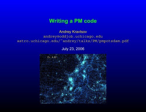
<strong>Writing</strong> a PM <strong>code</strong><br />
Andrey Kravtsov<br />
andrey@oddjob.uchicago.edu<br />
astro.uchicago.edu/˜andrey/talks/PM/<strong>pm</strong>potsdam.pdf<br />
July 23, 2006
Cosmological simulations 1<br />
Cosmological simulations: the problem<br />
• The Universe is thought to be composed of dark matter and normal matter<br />
(the baryons), photons, neutrinos, etc.<br />
• There should be ∼ 10 80÷90 particles of dark matter and baryons in the<br />
observable Universe.<br />
• In our Galaxy, the Milky Way, alone there are ∼ 10 68 baryonic particles.<br />
• Simulations, of course, cannot follow evolution of all of these particles.<br />
• The evolution of a large number of particles of a given type can be described<br />
as evolution of a continuous field, characterized by the distribution function<br />
f(x, ẋ, t) — the density of particles in phase space.
equations I 2<br />
Cosmological simulations: equations I<br />
• The evolution of f i is described by the Boltzmann equation:<br />
∂f i<br />
∂t + ẋ∂f i<br />
∂x + ẍ∂f i<br />
∂ẋ = C [f i, f j ] ;<br />
• C[f i , f j ] is the collision integral, describing possible particle collisions, which<br />
can scatter particles in and out of a phase-space volume. The form of C<br />
depends on the specific properties of particles in the system (i.e., how they<br />
scatter, whether they can be created or annihilated, etc.)<br />
• In general, a system of 6D Boltzmann equations (equations for each of the<br />
relevant components, i, of the Universe) needs to be solved.<br />
• This is indeed done in <strong>code</strong>s describing evolution of the primordial matter<br />
and linear perturbations to solve for the initial power spectrum and properties<br />
of the CMB temperature anisotropies. In this case, the matter distribution is<br />
close to uniform and no detailed information on the 3D distribution of matter<br />
is needed. The dimensionality of the problem can thus be reduced.
equations II 3<br />
Cosmological simulations: equations II<br />
• When solving for nonlinear structure formation, however, the full 3D spatial<br />
information is needed.<br />
• If dark matter is collisionless or nearly collisionless, C[f] = 0, resulting in<br />
a simpler, collisionless Boltzmann equation, a.k.a. the Vlasov equation.<br />
However, this “simpler” equation is still a 6D ODE, if we want to describe<br />
evolution of the matter in 3D space. High-dimensionality of the equation<br />
severely limits the resolution of simulations due to the large number of<br />
elements required to cover the 6D space.<br />
• The solution of the Vlasov equation can be represented in terms of<br />
characteristic equations, which look like equations of particle motion.<br />
Characteristic equations describe lines in phase space along which the<br />
distribution function is constant.<br />
• A complete set of characteristic equations is equivalent to the Vlasov<br />
equation. But if a representative subsample of characteristics can be<br />
followed, we can get the approximate evolution of the system.
N-body approach 4<br />
Cosmological simulations: N-body approach<br />
• This is the main idea behind the particle N-body approach in plasma and<br />
cosmological simulations.<br />
• In N-body approach, the initial phase space is split into small domains,<br />
each domain is represented by a particle, and particles are evolved selfconsistently<br />
using equations of particle motion:<br />
dx<br />
dt = u,<br />
du<br />
dt = −∇Φ<br />
with potential given by the Poisson equation:<br />
∇ 2 Φ = 4πGρ tot .<br />
• N-body approach is effectively a Monte Carlo technique for random<br />
sampling of the characteristics. 1<br />
1 Monte Carlo techniques are very often used in the otherwise intractable high-dimensional problems, like<br />
evaluating many-dimensional integrals or likelihood and parameter estimation in many-parameter problems.<br />
Markov Chain Monte Carlo (MCMC) methods are used in such problems.
particle initial conditions 5<br />
Cosmological simulations: particle initial conditions<br />
• If we deal with cold dark matter, initial particle velocities are due solely<br />
to gravity and, in the Zeldovich approximation, depend only on particle<br />
positions. In this case only 3D space needs to be discretized.<br />
• For other type of dark matter (hot, warm, etc.), their initial velocity distribution<br />
must also be sampled.<br />
• The problem of initial discretization is the problem of cosmological initial<br />
conditions, covered last week. For additional information see:<br />
Anatoly Klypin’s PM <strong>code</strong><br />
Ed Bertschinger’s GRAFIC2 package: a public cosmological IC <strong>code</strong><br />
Grocce et al. 2006, (astro-ph/0606505)<br />
• the number of particles and the size of simulation volume are dictated by the<br />
available computational resources and the needs of particular problem.
particle initial conditions 6<br />
Cosmological simulations: particle initial conditions<br />
“It seems probably to me that God in the beginning formed matter in solid,<br />
massy, hard, impenetrable, movable particles, of such sizes and figures, and<br />
with such other properties, and in such proportion to space, as most<br />
conduced to the end for which he formed them.”<br />
- Isaac Newton, “Opticks”
equations of gasdynamics 7<br />
Cosmological simulations: equations III: gasdynamics<br />
• In a fully collisional particle systems with properties of an ideal gas, the<br />
Boltzmann equation can be simplified and reduced to 3D ODEs describing<br />
ideal compressible gas.<br />
• This is done by taking the three first moments of the Boltzmann equations<br />
— i.e., multiplying the equation by 1, ẋ, and ẋ 2 and integrating over velocity<br />
space).
equations of gasdynamics 8<br />
Cosmological simulations: equations III: gasdynamics<br />
• These moments give the continuity, Euler, and energy equations of<br />
hydrodynamics 2 (e.g., F. Shu “Gasdynamics”):<br />
∂ρ<br />
∂t<br />
+ ∇ρu = 0,<br />
∂u<br />
∇P<br />
+ (u · ∇)u = −∇Φ −<br />
∂t ρ ,<br />
∂E<br />
+ ∇ · [(E + P )u] = −ρu · ∇Φ.<br />
∂t<br />
• The equations above are closed with the equation of state, which is usually<br />
assumed to be that of an ideal gas:<br />
ε = 1 P<br />
γ − 1 ρ ,<br />
or to have some other simple form (i.e., polytropic EoS: P = Kρ γ )<br />
2 Equations below do not take into account additional processes commonly included in simulations: heating<br />
and cooling of gas, star formation, etc. These are included as sink and source terms in the appropriate equations.<br />
We will consider such processes on friday.
equations summary 9<br />
Cosmological simulations: equations summary<br />
• Equations of particle motion, the Poisson equation, the equations of<br />
gasdynamics above, along with the equation of state of the gas, form the<br />
set of basic equations solved in cosmological simulations:<br />
dx<br />
dt = u,<br />
du<br />
dt = −∇Φ<br />
∇ 2 Φ = 4πGρ tot .<br />
∂E<br />
∂t<br />
∂u<br />
∂t<br />
∂ρ<br />
∂t<br />
+ ∇ρu = 0,<br />
+ (u · ∇)u = −∇Φ −<br />
∇P<br />
ρ ,<br />
+ ∇ · [(E + P )u] = −ρu · ∇Φ,<br />
ε = f(ρ, P ).
equations summary 10<br />
• Baryonic gas and dark matter are coupled by gravity, as they are both<br />
influenced by the same gravitational potential and they both contribute to<br />
the density in the Poisson equation.<br />
• Note that all of the equations we solve to describe the evolution of matter in<br />
the universe have their usual simple non-relativistic form. This is because<br />
most commonly the matter components relevant for late evolution move with<br />
non-relativistic velocities.
dissipationless simulations 11<br />
Cosmological simulations: dissipationless case<br />
• For many problems it is warranted to ignore the baryonic effects and solve<br />
only evolution of dissipationless component (dark matter, stars).<br />
• In this case, only equations of particle motion and the Poisson equation are<br />
solved.<br />
• Very generally, each evolution time step of a dissipationless simulation<br />
consists of the following two main parts:<br />
— gravity solver: solve the Poisson equation and calculate particle<br />
accelerations.<br />
— time integrator: update particle positions and velocities.<br />
• different <strong>code</strong>s differ in how these two parts are implemented.<br />
• Today we will consider the Particle-Mesh (PM) technique for solving the<br />
Poisson equation and integrating particle trajectories.
dissipationless simulations 12<br />
Particle-Mesh (PM) technique: a brief history<br />
• PM was invented in the 1950’s at LANL for simulations of compressible fluid<br />
flows<br />
• However, the first wide-spread application was for collisionless plasma<br />
simulations (for which PM was reinvented in the 1960’s and popularized by<br />
Hockney and collaborators)<br />
• In the late 70’s PM was first applied for 3D cosmological simulations. The<br />
method and its descendants (such as P 3 M, AP 3 M, and ART) have been<br />
used in most cosmological simulations ever since 3 .<br />
3 In the 1990’s Tree <strong>code</strong>s have also enjoyed increasing popularity
dissipationless simulations 13<br />
Particle-Mesh (PM) technique: modern relevance<br />
• The popularity of PM in cosmology is due to<br />
⋆ its relative algorithmic simplicity,<br />
speed (the running time scales as ∝ O(N p )+O(N c ln N c ), where N p is the<br />
number of particles and N c is the number of grid cells; and low storage<br />
requirements;<br />
⋆ natural incorporation of periodic boundary conditions;<br />
• Today the PM technique is still very much relevant because<br />
⋆ Simplicity allows for efficient parallelization → and thus simulation on<br />
largest distributed architectures;<br />
⋆ low storage requirements allow simulation of a very large numbers of<br />
particles with relatively low resolution, suitable for some problems (e.g.,<br />
halo mass function). Papers based on pure PM simulations still appear.<br />
⋆ PM technique is used to solve for the large-scale potential and forces in<br />
many modern high-resolution methods (e.g., AP 3 M, ART, TreePM 4 ).<br />
4 now implemented inthe Gadget-2 <strong>code</strong>
Model equations 14<br />
Model equations<br />
PM <strong>code</strong> solves the cosmological Poisson equation (Peebles 1980, LSS):<br />
∇ 2 Φ = 4πGρ tot − Λ,<br />
and equations of motion of particles<br />
dr<br />
dt = u;<br />
du<br />
dt = −∇Φ,<br />
note that all variables are defined in proper coordinates and all spatial<br />
derivatives are also taken with respect to these coordinates.
Model equations 15<br />
However, it is convenient to re-write the equations in comoving variables and<br />
make them dimensionless by choosing suitable units (I will denote variables in<br />
<strong>code</strong> units with a tilde˜). In the following, I will adopt the variables and units<br />
used in Anatoly Klypin’s PM <strong>code</strong>. This is just an example. Feel free to choose<br />
your own - just make sure you are consistent!<br />
˜x ≡ a −1 r r 0<br />
, ˜p ≡ a v v 0<br />
, ˜φ ≡<br />
φ<br />
φ 0<br />
, ˜ρ = a 3 ρ ρ 0<br />
,<br />
where x is the comoving coordinates, v = u − Hr = aẋ is the peculiar<br />
velocity 5 and φ is the peculiar potential defined as (Peebles 1980, p. 42)<br />
φ = Φ + 1/2 aä (r/a) 2 = Φ + H2 0<br />
2<br />
(Ω Λ,0 − 1 )<br />
2 a−3 Ω m,0 r 2 ,<br />
where<br />
Ω m,0 = 8πGρ 0<br />
3H0<br />
2 ; Ω Λ,0 = Λ<br />
3H0<br />
2 .<br />
5 p ∝ av is called momentum, this choice of variable allows us to get rid of the annoying (ȧ/a) terms in<br />
equations.
Model equations 16<br />
The quantities with subscript zero are the units in which corresponding<br />
physical variables are measured. The unit of length, r 0 , is an arbitrary scale. I<br />
will chose r 0 to be the size of the PM grid cell:<br />
r 0 = L box<br />
N g<br />
;<br />
N 3 g = total number of grid cells<br />
the rest of the units are defined as<br />
t 0 ≡ H −1<br />
0 ,<br />
v 0 ≡ r 0<br />
t 0<br />
,<br />
ρ 0 ≡ 3H2 0<br />
8πG Ω m,0,<br />
φ 0 ≡ r2 0<br />
t 2 0<br />
= v 2 0.
Model equations 17<br />
It is also convenient to choose the expansion factor as time variable (using<br />
expressions for the Hubble constant: ȧ = aH(a)). For this choice of variables,<br />
the Poisson equation and equations of motion can be re-written as<br />
∇ 2 φ = 4πGΩ m,0 ρ crit,0 a −1 δ,<br />
δ = ρ − ¯ρ<br />
¯ρ ,<br />
dp<br />
da = −∇φ ȧ ,<br />
dx<br />
da =<br />
p<br />
ȧa 2.<br />
where δ is the overdensity in comoving coordinates and ȧ is<br />
ȧ = H 0 a −1/2 √Ω m,0 + Ω k,0 a + Ω Λ,0 a 3 ; Ω m,0 + Ω Λ,0 + Ω k,0 = 1
Model equations 18<br />
In dimensionless variables the equations are:<br />
˜∇ 2 3Ω 0 ˜φ =<br />
2 a ˜δ,<br />
d˜p<br />
da<br />
= −f(a) ˜∇ ˜φ,<br />
d˜x<br />
da = f(a) ˜p a 2.<br />
where ˜δ = ˜ρ − 1 and<br />
f(a) ≡ H 0 /ȧ = [ a −1 ( Ω m,0 + Ω k,0 a + Ω Λ,0 a 3)] −1/2<br />
.<br />
These equations are used in the three main steps of a PM <strong>code</strong>:<br />
• Solve the Poisson equation using the density field estimated with current<br />
particle positions.<br />
• Advance momenta using the new potential.<br />
• Update particle positions using new momenta.
PM: main <strong>code</strong> blocks 19<br />
Data structures<br />
For a PM <strong>code</strong> with the second-order accurate time integration we need the<br />
minimum of six real numbers for positions and momenta for each particle<br />
(assuming particles have the same mass) and one real number for the<br />
potential of each grid cell.<br />
The array for the potential can be shared between density and potential: first<br />
use it for density, then replace it with potential when the Poisson equation is<br />
solved. However, for simplicity you can start with two grid arrays (for density<br />
and potential). Also, you will probably need auxiliary arrays for FFT,<br />
depending on which FFT solver you choose to use.<br />
The convenient data structures are 1D or 3D arrays for particles (e.g., six 1D<br />
arrays for x(i), y(i), z(i), vx(i), vy(i), vz(i)) and 3D arrays<br />
for the grid variables (e.g., rho(i,j,k), phi(i,j,k)).<br />
Run your tests for (32 3 , 64 3 ) or (64 3 , 128 3 ) particles and cells in which case<br />
memory requirements should not be an issue.
PM: main <strong>code</strong> blocks 20<br />
Density Assignment<br />
The Particle Mesh algorithms assume that particles have certain size, mass,<br />
shape, and internal density. This determines the interpolation scheme used to<br />
assign densities to grid cells. Let’s define the 1D particle shape, S(x), to be<br />
mass density at the distance x from the particle for cell size ∆x (Hockney &<br />
Eastwood 1981). The common choices are<br />
• Nearest Grid Point (NGP): particles are point-like and all of particle’s mass<br />
is assigned to the single grid cell that contains it:<br />
S(x) = 1 ( x<br />
)<br />
∆x δ ∆x<br />
• Cloud In Cell (CIC): particles are cubes (in 3D) of uniform density and of one<br />
grid cell size.<br />
S(x) = 1 {<br />
1, |x| <<br />
1<br />
2 ∆x<br />
∆x 0, otherwise
PM: main <strong>code</strong> blocks 21<br />
• Triangular Shaped Cloud (TSC):<br />
S(x) = 1<br />
∆x<br />
{<br />
1 − |x|/∆x, |x| < ∆x<br />
0, otherwise<br />
The fraction of particle’s mass assigned to a cell ijk is the shape function<br />
averaged over this cell:<br />
W (x p − x ijk ) =<br />
x ijk +∆x/2<br />
∫<br />
dx ′ S(x p − x ′ );<br />
x ijk −∆x/2<br />
W (r p − r ijk ) = W (x p − x ijk )W (y p − y ijk )W (z p − z ijk );<br />
The density in a cell ijk is then<br />
ρ ijk =<br />
N p<br />
∑<br />
p=1<br />
m p W (r p − r ijk )
PM: main <strong>code</strong> blocks 22<br />
In practice, of course, we loop over particles and assign the density to<br />
neighboring cells as opposed to summing over all particles for each cell as the<br />
straightforward reading of the above equation would suggest.
¡<br />
¡<br />
¡<br />
<br />
<br />
<br />
£ ¢<br />
¢<br />
£ ¢<br />
¢<br />
£ ¢<br />
¢<br />
¡<br />
¡<br />
¡<br />
<br />
¢ £<br />
'&( & <br />
¢ £<br />
.-0/ & <br />
¢ £<br />
<br />
<br />
<br />
¡<br />
¡<br />
¡<br />
<br />
<br />
<br />
<br />
<br />
<br />
<br />
<br />
¡<br />
¡<br />
¡<br />
PM: main <strong>code</strong> blocks 23<br />
PM interpolation kernels in real and Fourier space. Adopted from PM lectures by M.Gross<br />
3-9<br />
the density assignment wider in configuration space.<br />
¤¦¥¨§©<br />
¡ <br />
¡<br />
<br />
¤! #"$ %<br />
¡ <br />
¡<br />
<br />
¤*),+ %<br />
<br />
¡ <br />
¡
PM: main <strong>code</strong> blocks <strong>24</strong><br />
Implementing CIC interpolation<br />
The choice of interpolation scheme is a tradeoff between accuracy and<br />
computational expense. The CIC scheme is both relatively cheap and<br />
accurate and is most commonly used in PM <strong>code</strong>s. I will now describe how to<br />
implement it (you can start coding with the simpler NGP scheme and upgrade<br />
it to CIC later when your <strong>code</strong> is tested).<br />
Consider the density assignment for a particle with coordinates {x p , y p , z p }<br />
The cell containing the particle will have indices of<br />
i = [x p ]; j = [y p ]; k = [z p ],<br />
where [x] is the integer floor function (equivalent to Fortran’s int). Let’s<br />
assume that cell centers are at {x c , y c , z c } = {i, j, k} (note that in internal units<br />
cell size ∆x = 1, this will be implicitly assumed below). This is a matter of<br />
convention, but once chosen the convention should be consistent throughout<br />
the <strong>code</strong>.
PM: main <strong>code</strong> blocks 25<br />
In the CIC scheme, particle {x p , y p , z p } may contribute to densities in the<br />
parent cell (i, j, k) and seven neighboring cells 6 . Let’s define<br />
d x = x p − x c ; d y = y p − y c ; d z = z p − z c ;<br />
t x = 1 − d x ; t y = 1 − d y ; t z = 1 − d z .<br />
Contributions to the eight cells are then linear interpolations in 3D:<br />
ρ i,j,k = ρ i,j,k + m p t x t y t z ; ρ i+1,j,k = ρ i+1,j,k + m p d x t y t z ;<br />
ρ i,j+1,k = ρ i,j+1,k + m p t x d y t z ; ρ i+1,j+1,k = ρ i+1,j+1,k + m p d x d y t z ;<br />
ρ i,j,k+1 = ρ i,j,k+1 + m p t x t y d z ; ρ i+1,j,k+1 = ρ i+1,j,k+1 + m p d x t y d z ;<br />
ρ i,j+1,k+1 = ρ i,j+1,k+1 + m p t x d y d z ; ρ i+1,j+1,k+1 = ρ i+1,j+1,k+1 + m p d x d y d z ; ,<br />
where m p is particle mass. Doing this for all particles will result in the grid of<br />
densities ρ i,j,k .<br />
6 Make sure you enforce periodic boundary conditions: i = mod(i, Ng,1 ), etc. for j and k.
PM: main <strong>code</strong> blocks 26<br />
Solving the Poisson equation<br />
With the grid of densities, ρ i,j,k , in hand, the <strong>code</strong> can proceed to solve the<br />
discretized 7 Poisson equation<br />
˜∇ 2 ˜φ ≈ ˜φi−1,j,k + ˜φ i+1,j,k + ˜φ i,j−1,k + ˜φ i,j+1,k + ˜φ i,j,k−1 + ˜φ i,j,k+1 − 6 ˜φ i,j,k =<br />
= 3 Ω 0<br />
2 a (˜ρ i,j,k − 1).<br />
The discretization thus results in a large system of linear equations relating<br />
unknowns, ˜φ i,j,k , to the known right hand side values. This system can be<br />
solved using FFT.<br />
7 It is customary in PM <strong>code</strong>s to discretize the Laplacian operator using the 7-point template.
PM: main <strong>code</strong> blocks 27<br />
In the Fourier space the Poisson equation is ˜φ(k) = G(k)˜δ(k), where G(k) is<br />
the Green function which for the adopted discretization is given by<br />
G(k) = − 3Ω 0<br />
8a<br />
[ ( )<br />
sin 2 kx<br />
2<br />
( )<br />
+ sin 2 ky<br />
2<br />
( )] −1<br />
+ sin 2 kz<br />
,<br />
2<br />
where L = N g is the box size in <strong>code</strong> units and<br />
k x = 2πl/L, k y = 2πm/L, k z = 2πn/L, for component (l, m, n).<br />
The singularity at l = m = n = 0 should be avoided by setting this component<br />
of potential, ˆφ 000 , by hand to zero.
PM: main <strong>code</strong> blocks 28<br />
⇒ Given a density field ˜δ(r) in real space, we can solve for the gravitational<br />
potential by<br />
• performing the FFT to get ˜δ(k),<br />
• multiplying every element in the field by the corresponding value of G(k) to<br />
get ˜φ(k),<br />
ˆφ lmn = G(k lmn )ˆρ lmn , where<br />
N g −1<br />
∑<br />
ˆf lmn = (∆x) 3<br />
f ijk = 1 L 3<br />
i,j,k=0<br />
N g −1<br />
∑<br />
l,m,n=0<br />
f ijk e −i2π(il+jm+kn)/N g<br />
,<br />
ˆf lmn e i2π(il+jm+kn)/N g<br />
.<br />
• transforming 8 the result back to real space to get ˜φ(r) discretized at cell<br />
centers.<br />
8 Be careful about normalization of the FFT. The transforms ˜δ(r) → ˜δ(k) and ˜δ(k) → ˜δ(r) should recover the<br />
original field ˜δ(r).
PM: main <strong>code</strong> blocks 29<br />
Updating particle positions and velocities<br />
Let us assume we are using constant integration step in ∆a and the<br />
second-order accurate leapfrog integration.<br />
Schematic of the leapfrog integration for a variable time step. Note how<br />
velocities and particles are staggered in time. (adopted from M.Gross’s PM notes).
PM: main <strong>code</strong> blocks 30<br />
After n time steps, a n = a i + n∆a, during the step n + 1, we should have<br />
coordinates ˜x n at a n and momenta ˜p n−1/2 at a n−1/2 = a n − ∆a/2 from the<br />
previous step. Assigning density and solving the Poisson equation gives<br />
potential ˜φ n at a n . For the assumed variables and units, positions and<br />
momenta are updated as follows:<br />
˜p n+1/2 = ˜p n−1/2 + f(a n )˜g n ∆a;<br />
˜x n+1 = ˜x n + a −2<br />
n+1/2 f(a n+1/2)˜p n+1/2 ∆a.<br />
Here, ˜g n = − ˜∇ ˜φ n is acceleration at the particle’s position. This acceleration<br />
can be obtained by interpolating accelerations from the neighboring cell<br />
centers. The latter are given by<br />
˜g x i,j,k = −( ˜φ i+1,j,k − ˜φ i−1,j,k )/2, ˜g y i,j,k = −( ˜φ i,j+1,k − ˜φ i,j−1,k )/2,<br />
˜g z i,j,k = −( ˜φ i,j,k+1 − ˜φ i,j,k−1 )/2.
PM: main <strong>code</strong> blocks 31<br />
For each component of the acceleration, you should use the same<br />
interpolation scheme as during density assignment. For a given particle the<br />
acceleration should be interpolated from the cells to which particle contributed<br />
density during density assignment step. This is important! Consistency in<br />
interpolation schemes ensures absence of artificial self-forces and the third<br />
Newton’s law (Hockney & Eastwood 1981).<br />
For the NGP scheme, acceleration for a particle is just the acceleration of its<br />
parent cell ˜g i,j,k . For the CIC interpolation, we do the following (indices (i, j, k)<br />
here correspond to the parent cell of the particle; see section on density<br />
assignment).<br />
g x p = g x i,j,kt x t y t z + g x i+1,j,kd x t y t z + g x i,j+1,kt x d y t z + g x i+1,j+1,kd x d y t z +<br />
g x i,j,k+1t x t y d z + g x i+1,j,k+1d x t y d z + g x i,j+1,k+1t x d y d z + g x i+1,j+1,k+1d x d y d z .<br />
And the same for g p y and g p z. t x,y,z and d x,y,z have the same definition as in the<br />
CIC density assignment described above.<br />
After updating particle positions and velocities, the <strong>code</strong> should do some<br />
useful I/O and then proceed to step n + 2.
Zeldovich approximation (ZA) 32<br />
Zeldovich approximation<br />
• A first-order (linear) Lagrangian collapse model<br />
[Zeldovich 1970; see also Peacock’s (p. 485) and Padmanabhan’s (p. 294) textbooks for pedagogical introduction]<br />
• Zeldovich approximation can be expressed by one equation:<br />
x(t) = q + D + (t)S(q),<br />
it may look more familiar if you think about it as<br />
x(t) = x 0 + vt;<br />
v = const<br />
where<br />
q is the initial position of a matter parcel (a particle in N-body simulations) and<br />
x(t) is its position at time t (both q and x are comoving).<br />
D + (t) is the linear growth function [see eq. (29) in Carrol et al. (1993) for a useful fitting formula] and<br />
S(q) is a time-independent displacement vector.
Zeldovich approximation (ZA) 33<br />
• The evolution of density follows from conservation of mass ρ(x)d 3 x = ¯ρd 3 q :<br />
ρ(x, t) =<br />
¯ρ<br />
det(∂x j /∂q i ) =<br />
¯ρ<br />
det[δ ij + D + (t) × (∂S j /∂q i )]<br />
• ZA is exact in 1D until the first crossing of particle trajectories occurs. This<br />
is because in 1D ZA describes collapse of parallel sheets of matter and<br />
acceleration of each sheet is independent of x until sheets cross.<br />
• Although ZA is only an approximation in 3D, it still works very well at the<br />
initial stages of evolution of cosmological density fields because flattened<br />
pancake structures (whose evolution is well described by ZA) are typical in<br />
such fields 9 [see, e.g., Bond et al. (1996)]. This makes ZA the method of<br />
choice for setting up initial conditions in cosmological simulations.<br />
9 Another explanation of the success of ZA is its use of displacement field, S(q), as the basis for evolution<br />
model. Density depends on the derivatives of S(q) so that small (linear) displacements can correspond to large<br />
density contrasts.
A test problem: 1D collapse of a plane wave 34<br />
A test problem: 1D collapse of a plane wave<br />
• Let’s consider the evolution of a 1D sine-wave S(q) = A sin(kq):<br />
x(a) = q + D + (a)A sin(kq);<br />
k = 2π/λ;<br />
• Let’s assume we want to simulate a wave with wavelength equal to the<br />
simulation box size, λ = L box = N g using N 3 p,1 particles and N 3 g grid cells in<br />
a cubic grid. In 3D, the 1D equations can be used to set up initial conditions<br />
for N p,1 parallel sheets of particles. For some initial epoch, a ini , we have<br />
x i (a ini ) = q i + D + (a ini )A sin<br />
( ) 2πqi<br />
; q i = (i − 1) L box<br />
for i = 1, ..., N p,1 ;<br />
L box N p,1<br />
• Take the time derivative of x to get equation for peculiar velocity v = aẋ (or<br />
momentum p = av, if needed):<br />
v(x) = aḊ+(a ini − ∆a/2)A sin(kq),<br />
where initialization for the leapfrog scheme is assumed.
A test problem: 1D collapse of a plane wave 35<br />
• We can choose the first crossing epoch, say a cross = 10a ini . The epoch of<br />
the first crossing can then be identified as the epoch of the caustic formation<br />
(i.e., ρ(x cross , a cross ) = ∞, where x cross = q cross = L box /2), which gives us the<br />
wave amplitude A:<br />
ρ(x, a) =<br />
¯ρ<br />
[1 + D + (a) × Ak cos(kq)] , ⇒ A = − (D +(a cross )k) −1 .<br />
• Positions x(q, a) and velocities v(q, a) is all we need to set up initial<br />
conditions for particles.<br />
• The subsequent 1D evolution using the PM <strong>code</strong> can be tested by comparing<br />
x and v given by the above equations to the coordinates and velocities of<br />
particles at different epochs using outputs of your <strong>code</strong> (for example, you<br />
can plot phase diagrams, i.e. particles in v − x or v − q plane).
A test problem: 1D collapse of a plane wave 36<br />
• In addition, you can use solutions for the gravitational potential and particle<br />
accelerations to test your gravity solver. For each grid cell:<br />
φ(x, a) = 3 Ω 0<br />
2 a<br />
{ q 2 − x 2<br />
2<br />
}<br />
+ D + × Ak [kq sin(kq) + cos(kq) − 1] ;<br />
g(x, a) = − ∂φ<br />
∂x = 3 Ω 0<br />
2 a (x − q) = 3 Ω 0<br />
2 a D +(a)A sin(kq)<br />
The only difference from particles is that you do not know cell’s Lagrangian<br />
coordinate q (q is known for particles if you maintain particles in the same<br />
order throughout evolution; particle’s index gives q as we saw above). For<br />
a given expansion factor a, q of a cell can be calculated by solving equation<br />
q = x − D + (a)A sin(kq) numerically, with x is coordinate of the cell.
A test problem: 1D collapse of a plane wave 37<br />
Plane wave collapse test: phase diagram in Lagrangian coordinates q (a) the ART simulation with 32 3 base grid and 3<br />
refinement levels and (b) the PM simulation with a 32 3 -cell grid at the crossing time. Solid line, analytic solution; polygons,<br />
numerical results.(c,d) Corresponding phase diagram for physical coordinates x.
A test problem: 1D collapse of a plane wave 38<br />
Plane wave collapse test: rms deviations of (a) coordinates and (b) velocities from analytic solution vs. the expansion<br />
parameter for the PM <strong>code</strong> (solid line) and for the ART <strong>code</strong> with three levels of refinement (dashed line) See, Efstathiou et<br />
al. (1985) for details on this and other tests.
Setting up cosmological ICs 39<br />
Beyond the Zeldovich test:<br />
setting up cosmological initial conditions<br />
If your <strong>code</strong> passes the Zeldovich test, you may try to run a realistic<br />
cosmological simulation. To do this, you will have to <strong>code</strong> a routine to set up<br />
initial conditions for the particles using a statistical realization of the power<br />
spectrum, P (k), of your favorite cosmological model 10 . Fortunately, the basis<br />
for the algorithm is the now familiar ZA.<br />
The displacement of a particle is now determined not by a single wave, but by<br />
the entire set of waves that can be represented numerically in the simulation<br />
box. Thus, particle’s comoving coordinates and momenta, p = a 2 ẋ, are given<br />
by<br />
x = q − D + (a)S(q); p = −(a − ∆a/2) 2 Ḋ + (a − ∆a/2)S(q),<br />
where a is the initial expansion factor and ∆a is its step 11 , q is particle’s<br />
unperturbed position.<br />
10 An alternative is to set up initial conditions using a public <strong>code</strong>.<br />
11 Note that the growth factor D+ (a) is usually scale-independent (e.g., for all models with CDM only) and this<br />
is assumed here. This is not true, however, for some models, such as the Cold+Hot Dark Matter (CHDM).
Setting up cosmological ICs 40<br />
The displacement vector S is given by the discrete Fourier transform (e.g.,<br />
Padmanabhan 1993, p.294):<br />
S(q) = α<br />
k∑<br />
max<br />
k x,y,z =−k max<br />
ik c k exp (ik · q) ;<br />
k x,y,z = 2π<br />
N g<br />
l, m, n; l, m, n = 0, ±1, ..., ±N p,1 /2; k 2 = k 2 x + k 2 y + k 2 z ≠ 0.<br />
Here, α is the power spectrum normalization. The summation is over all<br />
possible wavenumbers from the fundamental mode with wavelentgh equal to<br />
the box size to the smallest “Nyquist” wavelength with the wavenumber of<br />
N p,1 /2. The real and imaginary components of the Fourier coefficients,<br />
c k = (a k − ib k )/2 are independent gaussian random numbers with the mean<br />
zero and dispersion σ 2 = P (k)/k 4 :<br />
a k = √ P (k)<br />
Gauss(0, 1)<br />
k 2 , b k = √ P (k)<br />
Gauss(0, 1)<br />
k 2 .<br />
Note that c k should satisfy condition c k = c ∗ −k = (a k − ib k )/2.
Setting up cosmological ICs 41<br />
Thus, if we construct a realization of {k x,y,z c k } using a cosmological power<br />
spectrum on a grid in the Fourier space, its discrete FFT gives us components<br />
of the real space displacement vector S(q) for all particles.
Setting up cosmological ICs 42<br />
Applying these equations in practice for N p particles on a cubic grid with N 3 g<br />
cells amounts to<br />
1) distributing particles uniformly in the simulation volume (e.g., placing<br />
particles in the centers of appropriately spaced grid cells).<br />
2) Computing the displacement vector for each particle position. Construct a<br />
realization of k x,y,z c k on three (each for one component of the wavevector)<br />
cubic grids. For example, for the x-component, the grid is initialized to k x c k<br />
where k x are running from −k Ny to k Ny (assume k Ny = N p,1 /2, k here is in<br />
units of the fundamental mode 2π/L box = 2π/Ng<br />
1/3 ) and a k and b k are<br />
gaussian random numbers defined above.<br />
3) FFT each of the three grids to get S x (q), S y (q), and S z (q) in real space.<br />
Apply ZA to displace particles from their Lagrangian positions (q → x).
Setting up cosmological ICs 43<br />
You will need<br />
• Your favorite FFT solver, if you don’t have one see Numerical Recipes (Ch.<br />
12).<br />
• A decent random number generator. Be careful here as you will need to<br />
generate fairly long sequences of random numbers (I can supply you with<br />
a RNG, if needed). The gaussian random pairs can be generated from<br />
the uniformly distributed numbers using the Box-Muller method (Numerical<br />
Recipes, Ch. 7).<br />
• A routine returning P (k) for a specific cosmological model. See Hu<br />
& Sugiyama 1996 and Eisenstein & Hu 1999 for useful analytical<br />
approximations to P (k).
project summary 44<br />
Project summary<br />
• use the blueprint given in this lecture to <strong>code</strong> up your own <strong>code</strong> (C or fortran).<br />
Use FFT routine given to you by Anatoly Klypin last week or a routine<br />
with more transparent packing (e.g., FFT routine from Ch.12 of “Numerical<br />
recipes”)<br />
• Test the <strong>code</strong> by simulating a sine-wave and comparing it to the Zeldovich<br />
solution<br />
• Set up an initial conditions for 64 3 /128 3 or 128 3 /256 3 particles/grid cells and<br />
run PM simulations in different cosmologies using the same random seed<br />
(which should give you the same phases and the same structures in these<br />
cosmologies):<br />
⋆ Ω 0 = 1 CDM universe with σ 8 = 0.8. Evolution of the growth factor in this<br />
model is simple: D + (a) = (a/a 0 ). You can check D + by computing the<br />
P (k) or two-point correlation function of DM particles at different epochs<br />
and comparing it to the expected evolution in linear regime.<br />
⋆ you can then simulate open CDM (Ω 0 = 0.3) and flat ΛCDM (Ω 0 = 0.3,<br />
Ω Λ = 0.7) with the same σ 8 (z = 0) = 0.8 as in the SCDM model above.
project summary 45<br />
• you can do various analyses of these simulations:<br />
⋆ plot particle distribution in slices<br />
⋆ plot P (k) at different representative stages of evolution<br />
⋆ run a halo finder (use yours or I can provide you with one) at different<br />
epochs and compare evolution of the mass function in these cosmologies.<br />
⋆ use your imagination! (e.g., parallelize your PM <strong>code</strong> with OpenMP)
References and links 46<br />
PM in cosmology: some historical references<br />
• Efstathiou G. & Eastwood J. 1981, MNRAS 194, 503<br />
• Klypin A.A. & Shandarin S.F. 1983, MNRAS 204, 891<br />
• Centrella J. & Melott A.L. 1983, Nature 305, 196-198<br />
• Miller R.H., 1983, ApJ 270, 390-409<br />
• Efstathiou G., Davis M., White S.D.M., & Frenk C.S. 1985, ApJS 57, <strong>24</strong>1-260
References and links 47<br />
Papers with useful info on PM<br />
• Hockney, R. W., and Eastwood, J. W. 1981, “Computer Simulation Using<br />
Particles”, McGraw-Hill, New York<br />
• Klypin A.A. & Shandarin S.F. 1983, MNRAS 204, 891<br />
• Efstathiou G., Davis M., White S.D.M., & Frenk C.S. 1985, ApJS 57, <strong>24</strong>1-260<br />
[Review and comparison of cosmological N-body methods]<br />
• Sellwood J.A. 1987, ARA&A 25, 151<br />
[Review of particle simulation methods]<br />
• Description of Hugh Couchman’s AP 3 M <strong>code</strong><br />
• Bertschinger E. 1998, ARA&A 36, 599<br />
[The most recent review of numerical techniques used in cosmological<br />
simulations and algorithms for setting up the initial conditions.]
References and links 48<br />
• Michael Gross’s, PhD Thesis<br />
[useful descriptions of PM and an algorithm for setting up ICs in Ch. 2 and<br />
Appendix A]<br />
• Klypin, A. & Holtzman, J. 1997, astro-ph/9712217<br />
”Particle-Mesh <strong>code</strong> for cosmological simulations”
References and links 49<br />
Web links<br />
• Amara’s Recap of Particle Simulation Methods: collection of info and links<br />
on various N-body algorithms<br />
• Anatoly Klypin’s public PM package for cosmological simulations.<br />
• Useful fortran (requires PGPLOT library) and C (requires OpenGL) <strong>code</strong>s<br />
for visualization of particle distributions in 3D.