Nominal Inversion Principles

Nominal Inversion Principles
Stefan Berghofer and Christian Urban
Technische Universität München
Institut für Informatik, Boltzmannstraße 3, 85748 Garching, Germany
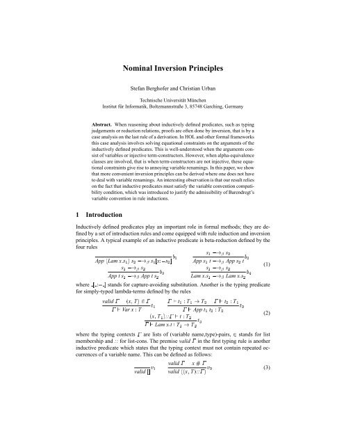
Abstract. When reasoning about inductively defined predicates, such as typing
judgements or reduction relations, proofs are often done by inversion, that is by a
case analysis on the last rule of a derivation. In HOL and other formal frameworks
this case analysis involves solving equational constraints on the arguments of the
inductively defined predicates. This is well-understood when the arguments consist
of variables or injective term-constructors. However, when alpha-equivalence
classes are involved, that is when term-constructors are not injective, these equational
constraints give rise to annoying variable renamings. In this paper, we show
that more convenient inversion principles can be derived where one does not have
to deal with variable renamings. An interesting observation is that our result relies
on the fact that inductive predicates must satisfy the variable convention compatibility
condition, which was introduced to justify the admissibility of Barendregt’s
variable convention in rule inductions.
1 Introduction
Inductively defined predicates play an important role in formal methods; they are defined
by a set of introduction rules and come equipped with rule induction and inversion
principles. A typical example of an inductive predicate is beta-reduction defined by the
four rules
s 1 ! s 2
App (Lam x:s 1 ) s 2 ! s 1 [x:=s 2 ] b 1
App s 1 t ! App s 2 t b 2
(1)
s 1 ! s 2
s 1 ! s 2
b 3 b 4
App t s 1 ! App t s 2 Lam x:s 1 ! Lam x:s 2
where [ := ] stands for capture-avoiding substitution. Another is the typing predicate
for simply-typed lambda-terms defined by the rules
valid (x; T) 2
` Var x : T
` t 1 : T 1 ! T 2 ` t 2 : T 1
t 1 t 2
` App t 1 t 2 : T 2
(2)
(x; T 1 ):: ` t : T 2
t 3
` Lam x:t : T 1 ! T 2
where the typing contexts are lists of (variable name,type)-pairs, 2 stands for list
membership and :: for list-cons. The premise valid in the first typing rule is another
inductive predicate which states that the typing context must not contain repeated occurrences
of a variable name. This can be defined as follows:
valid [] v 1
valid x #
valid ((x; T):: ) v 2 (3)

2 Stefan Berghofer and Christian Urban
where [] stands for the empty typing context and x # states that the variable name x
does not occur in .
The rule induction and inversion principles are the main thrust behind these definitions:
they provide the infrastructure for convenient reasoning about inductive predicates.
This is illustrated by the proof of the following lemma establishing that betareduction
preserves typing.
Lemma 1 (Type Preservation). If ` u : U and u ! u 0 then ` u 0 : U:
Type preservation can be proved by a rule induction on ` u : U. This gives rise to
three subgoals:
(i) Var x ! u 0 ^ : : : ) ` u 0 : T
(ii) App t 1 t 2 ! u 0 ^ : : : ) ` u 0 : T 2
(iii) Lam x:t ! u 0 ^ : : : ) ` u 0 : T 1 ! T 2
where we omitted some of the side-assumptions. The proof then proceeds by a case
analysis, called inversion, of the assumptions about ! .
In general, inversion is a reasoning principle that applies to any instance of an inductive
predicate occurring in the assumptions; it relies on the observation that this instance
must have been derived by at least one of the rules by which the inductive predicate is
defined. In informal reasoning one therefore matches the assumption with the conclusion
of every rule and tests whether the assumption and conclusion match. We will refer
to this kind of informal reasoning as inversion by matching and describe it next.
In the case (i), the assumption Var x ! u 0 matches with no conclusion in (1).
Therefore this is an impossible case, which implies that the goal ` u 0 : T holds trivially.
In the case (ii), the matching of App t 1 t 2 ! u 0 with the conclusions in (1) succeeds
in case of b 1 , b 2 and b 3 , and therefore three cases need to be considered. Let us
first analyse the case corresponding to the rule
s 1 ! s 2
App s 1 t ! App s 2 t b2
In this case we know for some s 2 that u 0 = App s 2 t 2 (since t 1 matches with s 1 , and
t with t 2 ). By induction we can infer that ` s 2 : T 1 ! T 2 and ` t 2 : T 1 hold.
Consequently, ` u 0 : T 2 holds.
Continuing with our informal reasoning, the case of beta-reduction, i.e. App (Lam
x:s 1 ) s 2 ! s 1 [x:=s 2 ], goes as follows: For some term s 1 , u 0 is equal to s 1 [x:=t 2 ] and
t 1 equal to Lam x:s 1 . The latter equation gives us that ` Lam x:s 1 : T 1 ! T 2 and
` t 2 : T 1 hold. To complete the proof we need the substitutivity lemma:
Lemma 2 (Type Substitutivity).
If (x; U):: ` t : T and ` u : U then ` t[x:=u] : T:
whose proof we omit. For this lemma to be useful, we have to invert the typing judgement
` Lam x:s 1 : T 1 ! T 2 . The informal inversion by matching gives us the desired
result: this judgement matches with the conclusion of the rule t 3 and we obtain
(x; T 1 ):: ` s 1 : T 2 . So we can conclude in this case by using Lemma 2 (similarly in
all remaining cases).

Nominal Inversion Principles 3
The point of these calculations is to show that the inversion by matching is very
natural and convenient. It is also very typical in programming language research: similar
proofs are described for System F

4 Stefan Berghofer and Christian Urban
8 x s 2 s 1: u 1 = App (Lam x:s 1) s 2 ^ u 2 = s 1[x:=s 2] ) P
8 s 1 s 2 t: u 1 = App s 1 t ^ u 2 = App s 2 t ^ s 1 ! s 2 ) P
8 s 1 s 2 t: u 1 = App t s 1 ^ u 2 = App t s 2 ^ s 1 ! s 2 ) P
8 s 1 s 2 x: u 1 = Lam x:s 1 ^ u 2 = Lam x:s 2 ^ s 1 ! s 2 ) P
u 1 ! u 2 ) P (4)
8 x T: ¡ = ^ u = Var x ^ U = T ^ valid ^ (x; T) 2 ) P
8 t 1 T 1 T 2 t 2: ¡ = ^ u = App t 1 t 2 ^ U = T 2 ^ ` t 1 : T 1 ! T 2 ^ ` t 2 : T 1 ) P
8 x T 1 t T 2: ¡ = ^ u = Lam x:t ^ U = T 1 ! T 2 ^ (x; T 1):: ` t : T 2 ) P
¡ ` u : U ) P (5)
Fig. 1. Inversion principles derived by Isabelle/HOL for the inductive predicates beta-reduction
and typing.
If we use inversion principle for ! (i.e. (4)) and invert Var x ! u 0 , we obtain the
following four subgoals:
8 x 0 s 2 s 1 : Var x = App (Lam x 0 :s 1 ) s 2 ^ u 0 = s 1 [x 0 :=s 2 ] ^ : : : ) ` u 0 : T
8 s 1 s 2 t: Var x = App s 1 t ^ u 0 = App s 2 t ^ s 1 ! s 2 ^ : : : ) ` u 0 : T
8 s 1 s 2 t: Var x = App t s 1 ^ u 0 = App t s 2 ^ s 1 ! s 2 ^ : : : ) ` u 0 : T
8 s 1 s 2 x 0 : Var x = Lam x 0 :s 1 ^ u 0 = Lam x 0 :s 2 ^ s 1 ! s 2 ^ : : : ) ` u 0 : T
The left-hand sides of these subgoals all reduce to False because the term constructors
are in conflict (Var can never be equal to App). Therefore we can quickly, like in the
informal reasoning, discharge all subgoals.
In case (ii) where we invert App t 1 t 2 ! u 0 , we obtain the following four subgoals:
8 x s 2 s 1 : App t 1 t 2 = App (Lam x:s 1 ) s 2 ^ u 0 = s 1 [x:=s 2 ] ^ : : : ) ` u 0 : T
8 s 1 s 2 t: App t 1 t 2 = App s 1 t ^ u 0 = App s 2 t ^ s 1 ! s 2 ^ : : : ) ` u 0 : T
8 s 1 s 2 t: App t 1 t 2 = App t s 1 ^ u 0 = App t s 2 ^ s 1 ! s 2 ^ : : : ) ` u 0 : T
8 s 1 s 2 x: App t 1 t 2 = Lam x:s 1 ^ u 0 = Lam x:s 2 ^ s 1 ! s 2 ^ : : : ) ` u 0 : T
The fourth subgoal can again be discharged because of the conflicting equality between
App and Lam. The reasoning in the second and third is very similar with the informal
inversion by matching, because the App-term constructor is injective and therefore we
can infer
App t 1 t 2 = App s 1 t ) t 1 = s 1 ^ t 2 = t; and
App t 1 t 2 = App t s 1 ) t 1 = t ^ t 2 = s 1
(6)
which are the same equations we would have got by the informal inversion by matching.
The first subgoal (corresponding to b 1 ) is more complicated: although we obtain by
injectivity of App the equations t 1 = Lam x:s 1 and t 2 = s 2 , we will encounter problems
with inverting the typing judgement ` Lam x:s 1 : T 1 ! T 2 . That is, we will not be
able to infer that (x; T 1 ):: ` s 1 : T 2 holds. This is because Lam is not injective and
we cannot reason as in (6).
We encounter the same problem with the reasoning in case (iii). There we have to
invert the reduction Lam x:t ! u 0 and obtain by using the first inversion principle
from (4) the following four subgoals:

Nominal Inversion Principles 5
8 x 0 s 2 s 1 : Lam x:t = App (Lam x 0 :s 1 ) s 2 ^ u 0 = s 1 [x 0 :=s 2 ] ) ` u 0 : T 1 ! T 2
8 s 1 s 2 t: Lam x:t = App s 1 t ^ u 0 = App s 2 t ^ s 1 ! s 2 ) ` u 0 : T 1 ! T 2
8 s 1 s 2 t: Lam x:t = App t s 1 ^ u 0 = App t s 2 ^ s 1 ! s 2 ) ` u 0 : T 1 ! T 2
8 s 1 s 2 x 0 : Lam x:t = Lam x 0 :s 1 ^ u 0 = Lam x 0 :s 2 ^ s 1 ! s 2 ) ` u 0 : T 1 ! T 2
Again the first three cases reduce to False. However in the fourth case we end up with
solving the equation
Lam x:t = Lam x 0 :s 1 (7)
where the variables x 0 and s 1 are universally quantified (that is we cannot choose them).
Since Lam is not injective, the only way to solve this equation is to unfold the definition
of alpha-equivalence, which in the Nominal Datatype Package gives us the cases
(i) x = x 0 ^ t = s 1 or
(ii) x 6= x 0 ^ t = (x x 0 )¡s 1 ^ x # s 1
where (x x 0 ) is a permutative renaming of x and x 0 , and x # s 1 stands for x not occurring
freely in s 1 , see [7]. While the first case is easy to deal with (the induction hypothesis
is immediately applicable), the second leads to the following proof state:
x 6= x 0 ^ x # s 1 ^ s 1 ! s 2 ^ : : : ) ` Lam x 0 :s 2 : T 1 ! T 2
with the induction hypothesis
8 s 0 : (x x 0 )¡s 1 ! s 0 ) (x; T 1 ):: ` s 0 : T 2
Here the formal reasoning starts to hurt, as it is much harder than the informal inversion
by matching. As one can see, the induction hypothesis is not directly applicable: we
know s 1 ! s 2 but we need that (x x 0 )¡s 1 reduces to some term. Also the induction
hypothesis gives us a typing-judgement involving the variable x, but we need one for x 0 .
The most direct way to complete this case requires the following side lemmas:
Lemma 3.
(i) If s 1 ! s 2 then (x x 0 )¡s 1 ! (x x 0 )¡s 2 .
(ii) If x # s 1 and s 1 ! s 2 then x # s 2 .
where, interestingly, the second is a property specific to beta-reduction.
Clearly, inverting Lam x:t ! u 0 in this way is not very convenient and the same
difficulties arise if we try to invert ` Lam x:s 1 : T 1 ! T 2 using (5) as needed in the
App-case above. In contrast, inverting inductive predicates based on the locally nameless
approach to binders (see [3]) is much simpler, because there all term constructors
are injective—even Lam. We show in this paper that we can obtain stronger inversion
principles (than given in Fig. 1), where they are stronger in the sense that we can avoid
the renaming of the binder, as long as the binder is sufficiently fresh. In this way we
can follow quite closely the informal reasoning of inversion by matching an assumption
with all rules.
These strong inversion principles will depend on the inductive predicates to satisfy
the variable convention compatibility condition, short vc-condition. The reason for
this condition is that the informal reasoning (i.e. inversion by matching) can lead to
faulty reasoning when alpha-equivalence classes are involved. Consider the following

6 Stefan Berghofer and Christian Urban
inductive definition of a two-place predicate (both arguments are alpha-equated lambdaterms)
Var x ,! Var x App t 1 t 2 ,! App t 1 t 2
t ,! t 0
Lam x:t ,! t 0 (8)
Now choose two distinct variables, say x and y with x 6= y. A simple calculation shows
that Lam x:Var x ,! Var x can be derived using the rules above. Therefore we can use it
as an assumption. Since we are working with alpha-equated lambda terms, we have that
Lam x:Var x = Lam y:Var y and therefore also Lam y:Var y ,! Var x must hold. Next
we apply the inversion principle naively to the latter instance of the relation, i.e. we
invert by matching this instance with the conclusions of the rules shown in (8). Only
the third rule matches, yielding the fact Var y ,! Var x. Next we invert this instance of
the relation: the first rule matches, enabling us to infer that x = y holds. This, however,
contradicts the assumption that x and y are distinct. The vc-condition will protect us
from this kind of faulty reasoning.
3 Inductive predicates
An inductive predicate, say R, is defined by a finite set of rules r i
B 1
R ts 1
r 1 : : :
B n
R ts n
r n (9)
where in the premises the B i are HOL-formulae possibly containing R and where in the
conclusion the ts i are the arguments of the predicate R. The ts i are HOL-terms, which
for the purposes of this paper we can assume to be either variables or constructed by
term constructors. Again for the purposes of this paper HOL-formulae will be the ones
given by the grammar
B ::= P ts j B 1 ^ B 2 j B 1 _ B 2 j B 1 ! B 2 j : B j 8 x: B x j 9 x: B x
where P stands for atomic predicates and ts are the arguments of P. In (9) we have
the usual assumption that the premises can contain the predicate R in positive position
only (see [1]). However, the B i can contain other predicates, these are usually called
side-conditions. For example our typing rule t 1 has the side-condition concerning 2
and valid as premise.
In what follows it is convenient to have the notations t[xs], where the xs contain all
the variables of t, and B[ys], where ys includes the free variables of B (in B some variables
might be bound because of the universal and existential quantifiers). The meaning
of a rule in (9) is then the implication
8 xs i : B i [xs i ] ) R ts[xs i ]
where each xs i includes all free variables in r i . That means every instantiation of the
free variables in r i will result in an instance of this rule. With the rules given in (9)
comes the following inversion principle

Nominal Inversion Principles 7
8 xs 1 : ss = ts 1 [xs 1 ] ^ B 1 [xs 1 ] ) P rule r 1
.
8 xs n : ss = ts n [xs n ] ^ B n [xs n ] ) P rule r n
R ss ) P
where the ts i correspond to the arguments in the conclusion of each rule and the B i to
the premises (not also that the xs i do not include any of the free variables in ss and P).
The inversion principles given for ! and the typing rues in Fig. 1 are instances of
(10). We refer to this inversion principle as the weak inversion principle. As we have
shown in Section 2: when applying the weak inversions to cases involving non-injective
term constructors, we need to analyse cases involving annoying variable renamings. We
will show later that a strong inversion principle can be derived from the weak one and
using the strong one we can avoid the renamings.
(10)
4 Nominal Logic Work
Before we proceed, we introduce some necessary notions from the nominal logic work
[7, 9]. We assume that there are countably infinitely many names, which can be used as
binders. We base our description on permutation actions and on the notion of support.
The support of an object will, for the purposes of this paper, coincides with the set of
free names of that object. For details and a proper definition of support see [8]. A name
a is fresh w.r.t. an object, say t, provided that it is not free in t; we write this as a # t.
Note that if t has finitely many free variables, then there exists a fresh variable w.r.t. t.
We will also use the auxiliary notation a # ts, in which ts stands for a collection of
objects t 1 ;: : : ;t n , to mean a # t 1 ,. . . , a # t n . We further generalise this notation to a
collection of names, namely as # ts, which means a 1 # ts,. . . , a m # ts.
Permutations are finite lists of swappings (i.e., pairs of variables). We write such
permutations as (a 1 b 1 )(a 2 b 2 ) ¡ ¡ ¡ (a n b n ); the empty list [] stands for the identity permutation,
list append (i.e. 1 @ 2 ) for the composition of two permutations and list
reversal (i.e.
1 ) for the inverse of a permutation. We define the permutation action
over the structure of types in HOL. The point of the permutation action is to push permutations
inside the structure of every object, renaming names on the way. A permutation
acting on names is therefore defined as follows:
[] ¡ a = a
(a; b):: ¡ c =
8
<
:
a if ¡ c = b
b if ¡ c = a
¡ c otherwise
The permutation action on lists, pairs and booleans is given by
(11)
¡ [] = []
¡ (x::xs) = ¡ x:: ¡ xs
¡ (x; y) = ( ¡ x; ¡ y)
¡ True = True
¡ False = False
(12)

8 Stefan Berghofer and Christian Urban
Notice the last two lines imply the fact that for every HOL-formula B the equality ¡
B = B holds. This is because HOL is a classical logic and every formula is either true
or false. For alpha-equated lambda-terms we have
¡ Var x = Var ( ¡ x)
¡ App t 1 t 2 = App ( ¡ t 1 ) ( ¡ t 2 )
¡ Lam x:t = Lam ( ¡ x):( ¡ t)
We can easily prove that the permutation actions in (11), (12) and (13) satisfy the following
three properties:
(i) [] ¡ ( ) = ( )
(ii) ( 1 @ 2 ) ¡ ( ) = 1 ¡ 2 ¡ ( )
(iii) If 1 2 then 1 ¡ ( ) = 2 ¡ ( ):
where in the last clause equality between two permutations, that is 1 2 , is defined
by the property that as 1 ¡ a = 2 ¡ a holds for all names a. In the next section we
need the following lemma about freshness and the permutation actions in (11), (12) and
(13):
Proposition 1. If a # ( ) and b # ( ) then (a b)¡( ) = ( ):
The notion of equivariance is derived from the permutation actions:
Definition 1 (Equivariance [7]). A HOL-term t, respectively a HOL-formula B, with
free variables amongst xs is equivariant provided for all , we have ¡ t[xs] = t[¡xs]
and ¡ B[xs] = B[¡xs].
From the definition of their permutation action, pairs, nil and list-cons are equivariant.
For HOL-formulae we have:
¡ (A ^ B) = ¡ A ^ ¡ B
¡ (A _ B) = ¡ A _ ¡ B
¡ (A ! B) = ¡ A ! ¡ B
¡ (: A) = : ¡ A
¡ (8 x: P x) = 8 x: ¡ P ( 1 ¡ x)
¡ (9 x: P x) = 9 x: ¡ P ( 1 ¡ x)
Therefore for all the structures we consider in this paper we can move permutations
inside the structures until they reach variables, therefore all structures we consider in
paper will be equivariant.
For proving our main result in the next section it is convenient to refine our notation
ts[xs] and B[xs] for indicating the free variables of ts and B. The reason is that some of
these variables stand for names and those names are potentially in binding positions.
By binding position we mean the x in Lam x:t. In what follows the notation ts[as;xs]
and B[as;xs] will be used to indicate that the variables in binding position of the ts
are included in as and the other variables of the ts are either in as or in xs (similarly
for HOL-formulae). We extend this notation also to rules: by writing r[as;xs] we mean
rules of the form
B[as;xs]
R ts[as;xs] r i[as;xs]
(13)
(14)
(15)

Nominal Inversion Principles 9
However, unlike in the notation for HOL-terms and HOL-formulae, we mean in r i [as;xs]
that the as stand exactly for the variables occurring somewhere in r i in binding position
and the xs stand for the rest of variables. To see how this notation works out in our
examples, reconsider the definitions for the relations given in (1) and (2). Using our
notation for these rules, we have
b 1 [x;s 1 ;s 2 ]
b 2 [ ;s 1 ;s 2 ;t]
b 3 [ ;s 1 ;s 2 ;t]
b 4 [x;s 1 ;s 2 ]
t 1 [ ; ;x;T]
t 2 [ ; ;t 1 ;t 2 ;T 1 ;T 2 ]
t 3 [x; ;t;T 1 ;T 2 ]
where ‘ ’ stands for no variable in binding position. An inductive definition for alphaequivalence
between lambda terms includes the two rules:
t 1 = t 2
Lam x:t 1 = Lam x:t 2
a 1
x 6= y t 1 = (x y)¡t 2 x # t 2
Lam x:t 1 = Lam y:t 2
a 2
There our notation would be a 1 [x;t 1 ;t 2 ] and a 2 [x;y;t 1 ;t 2 ].
5 Strengthening of the Inversion Principle
In this section, we show how the “weak” inversion rules in (10) can be used to derive
stronger inversion rules in which the equality constraints are formulated in such a way
that they can be solved without having to rename variables.
We have seen in the example about t ,! t 0 from the Introduction that inversion principles
involving alpha-equivalence classes require some care. In order to rule out the
problematic case (and similar ones), we need to impose a condition on the rules of an
inductive definition. It is interesting that the condition we impose is the same as the one
introduced in [8] for justifying the admissibility of Barendregt’s variable convention in
rule inductions.
A rule is said to be variable convention compatible, or short vc-compatible, provided
the following two properties are satisfied:
Definition 2 (Variable Convention Compatibility). A rule r[as;xs] with conclusion
R ts[as;xs] and premise B[as;xs] is vc-compatible provided that:
all HOL-terms and HOL-formulae occurring in r are equivariant, and
the premise B[as;xs] implies that as # ts[as;xs] holds and that the as are distinct.
Note that if rule r does not contain any variable in binding position, then the second
condition is vacuously true. The first condition ensures that the relation R is equivariant.
The equivariance property will allow us to push permutations inside HOL-terms and
HOL-formulae until they reach free variables.

10 Stefan Berghofer and Christian Urban
If every introduction rule in an inductive definition satisfies these conditions, then
the inversion principle can be strengthened. The strengthened version looks as follows
8 xs 1 : (bs 1 # ss ^ distinct(bs 1 ) ) ss = ts 1 [bs 1 ;xs 1 ] ^ B 1 [bs 1 ;xs 1 ]) ) P rule r 1
.
8 xs n : (bs n # ss ^ distinct(bs n ) ) ss = ts n [bs n ;xs n ] ^ B n [bs n ;xs n ]) ) P rule r n
R ss ) P
(16)
where for every rule r 1 ;: : : ;r n we have a case to analyse. In our notation the rules have
the form r 1 [bs 1 ;xs 1 ];: : : ;r n [bs n ;xs n ] where the bs i are the variables in binding position.
Note that in contrast to (10) the variables bs i are no longer universally quantified, meaning
that we are free to choose the names bs i when we want to invoke the strong inversion
principle. The only constraints we have is that the preconditions bs i # ss ^ distinct(bs i )
need to be satisfied. This will be the case if the bs i are sufficiently fresh.
We now prove the main result of this paper: if the rules of an inductive definition
are vc-compatible, then the strong inversion principle in (16) holds.
Theorem 1. For an inductive definition of the predicate R, involving vc-compatible
rules only, a strong inversion principle exists deriving the implication R ss ) P.
Proof. We need to establish R ss ) P using the implications indicated in (16). To do
so we will use the weak inversion rule from (10). For each rule r i [as i ;xs i ] of the form
we have to analyse one case of the form
B[as i ;xs i ]
R ts i [as i ;xs i ]
8 as i xs i : ss = ts i [as i ;xs i ] ^ B i [as i ;xs i ] ) P
To show P in these cases we have available the fact from (16), namely
8 xs i : (bs i # ss ^ distinct(bs i ) ) ss = ts i [bs i ;xs i ] ^ B i [bs i ;xs i ]) ) P (17)
We first assume that
ss = ts i [as i ;xs i ] (18)
B i [as i ;xs i ] (19)
hold. Since r i [as i ;xs i ] is assumed to be vc-compatible, we further have that
(a) as i # ts i [as i ;xs i ] and (b) distinct(as i ) (20)
hold. The proof then proceeds by choosing for every name a in as i a fresh name c such
that for all the cs i the following hold (cs i is the collection of all those c):
(a) cs i # ss (b) cs i 6= as i (c) cs i 6= bs i (d) distinct(cs i ) (21)

Nominal Inversion Principles 11
Such a sequence cs i always exists: the first three properties can be obtained since the
terms ss, as i and bs i stand for finitely supported objects—so a free variable always
exists; the last can be obtained by choosing the c one after another avoiding the ones
that have already been chosen. We now build the permutation
def = (b n c n ): : : (b 1 c 1 ) (a n c n ): : : (a 1 c 1 )
The point of is that when applied to the as i we get ¡ as i = bs i . This follows from
the properties in (20.b), (21.b-d) and the fact that we can assume distinct(bs i ) holds
(see below). We next instantiate in (17) the xs i with ¡ xs i giving us
(bs i # ss ^ distinct(bs i ) ) ss = ts i [bs i ; ¡ xs i ] ^ B i [bs i ; ¡ xs i ]) ) P
So in order to show P, it suffices to prove
under the assumptions
ss = ts i [bs i ; ¡ xs i ] ^ B i [bs i ; ¡ xs i ] (22)
(a) bs i # ss and (b) distinct(bs i ) (23)
From (23.a) and (18) we obtain bs i # ts i [as i ;xs i ]. Using this, (20.a) and Lemma 1,
we have that ¡ ts i [as i ;xs i ] = ts i [as i ;xs i ]. Since the rule is equivariant we have that
¡ ts i [as i ;xs i ] = ts i [bs i ; ¡ xs i ] and thus also the first conjunct of (22). The reasoning
for the other conjunct is as follows: using (19) and the fact that B i is a boolean we have
that ¡ B i [as i ;xs i ] holds. Again by equivariance of the rule, we can move the permutation
inside to obtain B i [bs i ; ¡ xs i ]—the second conjunct of (22). This concludes the
proof.
ut
Let us next describe how the stronger inversion principles simplify the formal reasoning
in the type preservation lemma.
6 Examples
To use the strong inversion rules, we first have to make sure that the beta-reduction
and typing relation are equivariant. For this we only have to observe that all constants
(that is term constructors and functions) in the rules of ! , typing and valid are
equivariant. This follows either from the definition of the permutation action or is by
a simple induction over the predicates (in our implementation Isabelle will infer this
automatically). To show that the second condition in Definition 2 is satisfied we have to
show that the binders are fresh w.r.t. the conclusions of the rule they appear in. That is
a simple calculation for the rules
(x; T 1 ):: ` t : T 2
` Lam x:t : T 1 ! T 2
t 3
s 1 ! s 2
Lam x:s 1 ! Lam x:s 2
b 4

12 Stefan Berghofer and Christian Urban
8 s 2 s 1: (y # (u 1; u 2) ) u 1 = App (Lam y:s 1) s 2 ^ u 2 = s 1[y:=s 2] ^ y # s 2) ) P
8 s 1 s 2 t: u 1 = App s 1 t ^ u 2 = App s 2 t ^ s 1 ! s 2 ) P
8 s 1 s 2 t: u 1 = App t s 1 ^ u 2 = App t s 2 ^ s 1 ! s 2 ) P
8 s 1 s 2: (x # (u 1; u 2) ) u 1 = Lam x:s 1 ^ u 2 = Lam x:s 2 ^ s 1 ! s 2) ) P
u 1 ! u 2 ) P (24)
8 x T: ¡ = ^ u = Var x ^ U = T ^ valid ^ (x; T) 2 ) P
8 t 1 T 1 T 2 t 2: ¡ = ^ u = App t 1 t 2 ^ U = T 2 ^ ` t 1 : T 1 ! T 2 ^ ` t 2 : T 1 ) P
8 T 1 t T 2: (x # (¡; u; U) ) ¡ = ^ u = Lam x:t ^ U = T 1 ! T 2 ^ (x; T 1):: ` t : T 2) ) P
¡ ` u : U ) P
Fig. 2. Strong inversion principles derived by the Nominal Datatype Package for the inductive
predicates for beta reduction and typing.
(25)
In the first case we have to show that x # ( ; Lam x:t; T 1 ! T 2 ) holds under the
assumption that (x; T 1 ):: ` t : T 2 . Since we can show by a routine induction that
typing judgements only include valid contexts, we have that valid ((x; T 1 ):: ) holds.
From this we can infer that x # . We also know that x # Lam x:t (since x is abstracted)
and that x # T 1 ! T 2 (since types in the simply-typed lambda-calculus do not contain
any variables). We can discharge the conditions in the other rule by similar arguments.
However the condition will fail for the rule
b1 (26)
App (Lam x:s 1 ) s 2 ! s 1 [x:=s 2 ]
because we cannot determine whether x # s 2 . However we can show that this betareduction
rule is equivalent to the following more restricted rule
x # s 2
App (Lam x:s 1 ) s 2 ! s 1 [x:=s 2 ] b0 1 (27)
This is because we can choose a y such that y # (s 1 ; s 2 ) and alpha-rename App (Lam
x:s 1 ) s 2 to App (Lam y:(y x)¡s 1 ) s 2 . Then apply the restricted rule to this term in order
to obtain the reduct ((y x)¡s 1 )[y:=s 2 ]. By a structural induction over s 1 , we can show
that this term is equal to s 1 [x:=s 2 ] as desired. The point of this “manoeuvre” is that we
can show that the restricted rule for beta-reduction does satisfy the vc-condition.
The result of these calculations is that there are strengthened inversion rules for
beta-reduction and the typing-relation. They are given in Fig. 2. Using them for the type
preservation lemma, the second and third case are the same as with the weak inversion
rule (4). In the first and fourth case, however, the user does not need to show the claim
for an arbitrary variable x 0 , but for a sufficiently freshly chosen one (it has to be fresh
w.r.t. (u 1 ; u 2 )). In the strong inversion for the typing rule we have that the cases for
variables and applications are the same as with the weak inversion rule (5). In the case
of lambda abstractions, the user can choose a x so that x # (¡; u; U). These choices
will hugely simplify the formal reasoning. To give an impression of this fact we show
next three lemmas in Isabelle/HOL proving special instances of inversion principles.

Nominal Inversion Principles 13
lemma Ty-Lam-inversion:
assumes ty: ` Lam x.t : T and fc: x#
shows 9 T 1 T 2: T = T 1 ! T 2 ^ (x;T 1):: ` t : T 2
using ty fc by (cases rule: typing:strong-cases) (auto simp add: alpha)
lemma Beta-Lam-inversion:
assumes red: Lam x.t ! s and fc: x#s
shows 9 t 0 : s = Lam x.t 0 ^ t ! t 0
using red fc by (cases rule: Beta:strong-cases) (auto simp add: alpha)
lemma Beta-App-inversion:
assumes red: App (Lam x.t) s ! r and fc: x#(s;r)
shows (9 t 0 : r = App (Lam x.t 0 ) s ^ t ! t 0 ) _
(9 s 0 : r = App (Lam x.t) s 0 ^ s ! s 0 ) _ (r = t[x:=s])
using red fc
by (cases rule: Beta:strong-cases) (auto dest: Beta-Lam-inversion simp add: alpha)
These lemmas are needed frequently in proofs about structural operational semantics.
As seen in Section 2, it would have been quite painful to derive them using the weak
inversion principles. We use the alpha-rule in the proofs above in order to rewrite the
trivial alpha-equivalence Lam x:t = Lam x:s to t = s.
The Isar-proof of the complete type preservation lemma is given in Fig. 3. Lines 6
and 7 show the variable case. Lines 9-21 contain the steps for the case where a betareduction
occurs (the other cases are automatic in Line 22). We first chose a fresh name
x (Line 10); invert App t 1 t 2 ! u 0 in Line 12 using the fresh x. In the only interesting
case, we have that ` Lam x:s 1 : T 1 ! T 2 holds (Line 15), which we can invert to
(x; T 1 ):: ` s 1 : T 2 . To this we can apply the Lemma 2 (Line 20). In the lambda-case
(Lines 24-31), we invert Lam x:t ! u 0 . We know that x is fresh for u 0 by the strong
induction (Line 5). We can apply the induction hypothesis in Line 28 and use the typing
rule to conclude (Lines 30 and 31).
7 Conclusion and Related Work
As long as one is dealing with injective term constructors, the weak (or standard) inversion
rules provided by Isabelle/HOL work similarly to the informal inversion by matching
an assumption over the conclusions of inference rules. However, non-injective term
constructors, such as Lam in the lambda-calculus, give rise to annoying variable renamings,
and formal reasoning is quite different from and much more inconvenient than
the informal inversion by matching. This was observed in [3], because in their locally
nameless representation of binders, all term constructors are injective.
We have shown in this paper that if a binder is fresh with respect to the conclusion
of the rule where the binder appears and the inductive predicate satisfies the vccondition,
then one can avoid the renamings. As a result the formal inversion principles
are again as convenient the informal reasoning of inversion by matching—though the
strong inversion principles only apply to vc-compatible inductive relations. In (8) we
have shown that the informal inversion by matching can lead to faulty reasoning when
the vc-condition is not satisfied. In our implementation this kind of faulty reasoning is

26
14 Stefan Berghofer and Christian Urban
1 lemma type-preservation:
2 assumes ty: ` u : U and red: u ! u 0
3 shows ` u 0 : U
4 using ty red
5 proof (nominal-induct avoiding: u 0 rule: typing:strong-induct)
6 case (ty-Var x T)
7 from h Var x ! u 0 i show ` u
0
: T by (cases) (simp-all)
8 next
9 case (ty-App t 1 T 1 T 2 t 2)
10 obtain x::name where fc: x # ( ; App t 1 t 2; u 0 ) by (rule exists-fresh-var)
11 from h App t1 t 2 ! u 0 i show ` u
0
: T 2 using fc
12 proof (cases rule: Beta:strong-cases[where x=x and xa=x])
13 case (Beta s 2 s 1)
14 then have eqs: t 1 = Lam x.s 1 t 2 = s 2 u 0 = s 1[x:=s 2] using fc by (simp-all)
15 from h ` t 1 : T 1 ! T 2 i have ` Lam x.s1 : T 1 ! T 2 using eqs by simp
16 then have (x;T 1):: ` s 1 : T 2 using fc
17 by (cases rule: typing:strong-cases) (auto simp add: alpha)
18 moreover
19 from h ` t 2 : T 1 i have ` s2 : T 1 using eqs by simp
20 ultimately have ` s 1[x:=s 2] : T 2 by (rule type-substitutivity)
21 then show ` u 0 : T 2 using eqs by simp
22 qed (auto intro: ty-App)
23 next
24 case (ty-Lam x T 1 t T 2)
25 from h Lam x.t ! u 0 i h x # u
0 i
obtain s 2 where t-red: t ! s 2 and eq: u 0 = Lam x.s 2
27 by (cases rule: Beta:strong-cases) (auto simp add: alpha)
28 have ih: t ! s 2 =) (x;T 1):: ` s 2 : T 2 by fact
29 with t-red have (x;T 1):: ` s 2 : T 2 by simp
30 then have ` Lam x.s 2 : T 1 ! T 2 by (rule typing:ty-Lam)
31 with eq show ` u 0 : T 1 ! T 2 by simp
32 qed
Fig. 3. An Isar-proof of the type preservation lemma in Isabelle/HOL.
prevented because the strong inversion principles are derived only when the user has
verified the second part of the vc-condition (see Def. 2); the first part of that condition
is verified automatically by observing that equivariant inductive predicates must be
composed of equivariant components only.
What was surprising to us is that the strong inversion principles depend on the vccondition
that we introduced in previous work [8]. There, this condition was used to
make sure that the variable convention in proofs by rule induction does not lead to
faulty lemmas. An disadvantage of our approach is that in case of beta-reduction we
have to use rule b 0 shown in (27) and so far we have no automatic method to derive
1
from it the usual rule b 1 shown in (26).
The most closely related work to the one presented here is our own [8], where we
study strong induction principles. Here we were concerned with inversion principles,
which in our setting with non-injective term constructors are not a degenerated form

Nominal Inversion Principles 15
of induction (as is usually the case). In contrast with that work [8], we also deal here
with the case where rules include quantifiers. In the context of type theory, inversion
principles have been studied by Cornes and Terrasse for the Coq proof assistant [4]
and by McBride for the LEGO system [5]. McBride’s implementation in LEGO uses
an algorithm for solving equality constraints based on unification. The derivation of
inversion principles for inductive sets in Isabelle’s object logic HOL and ZF was first
described by Paulson [6].
References
1. P. Aczel. An Introduction to Inductive Definitions. In J. Barwise, editor, Handbook of Mathematical
Logic, pages 739–782. Elsevier, 1977.
2. B. E. Aydemir, A. Bohannon, M. Fairbairn, J. N. Foster, B. C. Pierce, P. Sewell, D. Vytiniotis,
G. Washburn, S. Weirich, and S. Zdancewic. Mechanized Metatheory for the Masses:
The POPLMARK Challenge. In T. Melham and J. Hurd, editors, Theorem Proving in Higher
Order Logics: TPHOLs 2005, LNCS. Springer-Verlag, 2005. Available electronically at
http://www.cis.upenn.edu/plclub/wiki-static/poplmark.pdf.
3. B. E. Aydemir, A. Charguéraud, B. C. Pierce, R. Pollack, and S. Weirich. Engineering formal
metatheory. In G. C. Necula and P. Wadler, editors, Proceedings of the 35th ACM SIGPLAN-
SIGACT Symposium on Principles of Programming Languages, POPL 2008, San Francisco,
California, USA, January 7-12, 2008, pages 3–15. ACM, 2008.
4. C. Cornes and D. Terrasse. Automating Inversion of Inductive Predicates in Coq. In S. Berardi
and M. Coppo, editors, Types for Proofs and Programs, International Workshop TYPES’95,
Torino, Italy, June 5-8, 1995, Selected Papers, volume 1158 of Lecture Notes in Computer
Science, pages 85–104. Springer, 1996.
5. C. McBride. Inverting Inductively Defined Relations in LEGO. In E. Giménez and C. Paulin-
Mohring, editors, Types for Proofs and Programs, International Workshop TYPES’96, Aussois,
France, December 15-19, 1996, Selected Papers, volume 1512 of Lecture Notes in Computer
Science, pages 236–253. Springer, 1998.
6. L. C. Paulson. A fixedpoint approach to (co)inductive and (co)datatype definitions. In
G. Plotkin, C. Stirling, and M. Tofte, editors, Proof, Language, and Interaction: Essays in
Honor of Robin Milner, pages 187–211. MIT Press, 2000.
7. A. M. Pitts. Nominal Logic, A First Order Theory of Names and Binding. Information and
Computation, 186:165–193, 2003.
8. C. Urban, S. Berghofer, and M. Norrish. Barendregt’s Variable Convention in Rule Inductions.
In F. Pfenning, editor, 21st International Conference on Automated Deduction (CADE-21),
volume 4603 of Lecture Notes in Artificial Intelligence, pages 35–50. Springer-Verlag, 2007.
9. C. Urban and C. Tasson. Nominal Techniques in Isabelle/HOL. In Proc. of the 20th International
Conference on Automated Deduction (CADE), volume 3632 of LNCS, pages 38–53,
2005.