Upgrade Report - Department of Informatics - King's College London
Upgrade Report - Department of Informatics - King's College London
Upgrade Report - Department of Informatics - King's College London
- No tags were found...

You also want an ePaper? Increase the reach of your titles
YUMPU automatically turns print PDFs into web optimized ePapers that Google loves.
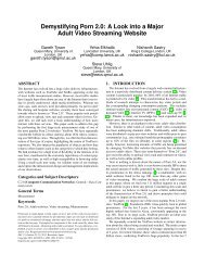
King’s <strong>College</strong> <strong>London</strong><strong>Department</strong> <strong>of</strong> <strong>Informatics</strong>Algorithm Design Group<strong>Report</strong> Submitted for <strong>Upgrade</strong> to PhDAuthorYiannis SiantosS.N: 0972443SupervisorsDr. Colin CooperDr. Tomasz RadzikFebruary 28, 2012
ContentsI Introduction 21 Online Social Networks (OSNs) 22 Large Online Social Networks and Generative Models 33 Graph sampling and crawling 3II Related Work 44 Network properties and metrics 44.1 Diameter and degree distribution . . . . . . . . . . . . . . . . . . . . . . . . . . . . . . . . . . 44.2 Degree correlations . . . . . . . . . . . . . . . . . . . . . . . . . . . . . . . . . . . . . . . . . . 44.3 Expander graphs . . . . . . . . . . . . . . . . . . . . . . . . . . . . . . . . . . . . . . . . . . . 44.4 Connected Components And Community Structure . . . . . . . . . . . . . . . . . . . . . . . . 54.5 Communities: Conductance . . . . . . . . . . . . . . . . . . . . . . . . . . . . . . . . . . . . . 54.6 Communities: Centrality and modularity . . . . . . . . . . . . . . . . . . . . . . . . . . . . . 64.7 Communities: Overlapping communities . . . . . . . . . . . . . . . . . . . . . . . . . . . . . . 64.8 Property testing . . . . . . . . . . . . . . . . . . . . . . . . . . . . . . . . . . . . . . . . . . . 75 Graph Generation Models 75.1 Erdós-Rényi Graph . . . . . . . . . . . . . . . . . . . . . . . . . . . . . . . . . . . . . . . . . . 75.2 Preferential attachment model . . . . . . . . . . . . . . . . . . . . . . . . . . . . . . . . . . . 85.3 Edge Copying model . . . . . . . . . . . . . . . . . . . . . . . . . . . . . . . . . . . . . . . . . 95.4 Triangle Closing Model . . . . . . . . . . . . . . . . . . . . . . . . . . . . . . . . . . . . . . . 115.5 Forest Fire Model . . . . . . . . . . . . . . . . . . . . . . . . . . . . . . . . . . . . . . . . . . . 115.6 Stochastic Kronecker Graph . . . . . . . . . . . . . . . . . . . . . . . . . . . . . . . . . . . . . 125.7 Affiliation Networks . . . . . . . . . . . . . . . . . . . . . . . . . . . . . . . . . . . . . . . . . 136 Graph sampling and crawling 146.1 Simple Random Walk . . . . . . . . . . . . . . . . . . . . . . . . . . . . . . . . . . . . . . . . 166.2 Weighted Random Walk . . . . . . . . . . . . . . . . . . . . . . . . . . . . . . . . . . . . . . . 176.3 Metropolis Hastings Random Walks (MHRWs) . . . . . . . . . . . . . . . . . . . . . . . . . . 17III Our Work 197 Graph generation 197.1 Random Walk Graph . . . . . . . . . . . . . . . . . . . . . . . . . . . . . . . . . . . . . . . . . 197.2 Preferential attachment and message propagation . . . . . . . . . . . . . . . . . . . . . . . . . 207.3 Grow, Back-Connect, Densify . . . . . . . . . . . . . . . . . . . . . . . . . . . . . . . . . . . . 217.4 Implicit Graph Model . . . . . . . . . . . . . . . . . . . . . . . . . . . . . . . . . . . . . . . . 22I
7.5 Partitioned Preferential Attachment . . . . . . . . . . . . . . . . . . . . . . . . . . . . . . . . 248 Existing Data Set Analysis 258.1 Ground truth. Complete twitter snapshot . . . . . . . . . . . . . . . . . . . . . . . . . . . . . 258.2 Other Real Networks . . . . . . . . . . . . . . . . . . . . . . . . . . . . . . . . . . . . . . . . . 268.2.1 Degree Distributions . . . . . . . . . . . . . . . . . . . . . . . . . . . . . . . . . . . . . 278.2.2 Degree-Based Cut Conductunce . . . . . . . . . . . . . . . . . . . . . . . . . . . . . . . 288.2.3 Degree Correlations . . . . . . . . . . . . . . . . . . . . . . . . . . . . . . . . . . . . . 299 Graph Sampling 299.1 Sampling Real World Networks: Case study <strong>of</strong> twitter . . . . . . . . . . . . . . . . . . . . . . 299.1.1 Our initial crawling . . . . . . . . . . . . . . . . . . . . . . . . . . . . . . . . . . . . . 309.1.2 Second crawling, unbiased sampling . . . . . . . . . . . . . . . . . . . . . . . . . . . . 309.2 Uniform Sampling (UNI): A study <strong>of</strong> efficiency . . . . . . . . . . . . . . . . . . . . . . . . . . 329.3 Sampling Manufactured Graphs: Weighted Random Walk . . . . . . . . . . . . . . . . . . . . 339.3.1 Theoretical foundation . . . . . . . . . . . . . . . . . . . . . . . . . . . . . . . . . . . . 339.3.2 Experimental results . . . . . . . . . . . . . . . . . . . . . . . . . . . . . . . . . . . . . 37IV Future Work 4110 Graph Analysis 4110.1 Real world network characteristics . . . . . . . . . . . . . . . . . . . . . . . . . . . . . . . . . 4110.2 Property Testing and Estimation Algorithms . . . . . . . . . . . . . . . . . . . . . . . . . . . 4211 Graph sampling 4211.1 Algorithm Optimizations . . . . . . . . . . . . . . . . . . . . . . . . . . . . . . . . . . . . . . 4311.1.1 Algorithm complexity reduction . . . . . . . . . . . . . . . . . . . . . . . . . . . . . . 4311.1.2 Run-time reduction . . . . . . . . . . . . . . . . . . . . . . . . . . . . . . . . . . . . . 4311.1.3 Approximation . . . . . . . . . . . . . . . . . . . . . . . . . . . . . . . . . . . . . . . . 4411.2 Improvement Of Sampling Efficiency . . . . . . . . . . . . . . . . . . . . . . . . . . . . . . . . 4412 Graph Generation models 44V References 4613 Acronyms 49VI Appendix 50A Sampling Manufactured Graphs: BFS Tree Filtering 50A.1 Crawler Definitions . . . . . . . . . . . . . . . . . . . . . . . . . . . . . . . . . . . . . . . . . . 50A.2 Measured properties . . . . . . . . . . . . . . . . . . . . . . . . . . . . . . . . . . . . . . . . . 50A.2.1 Crawlers With Memory . . . . . . . . . . . . . . . . . . . . . . . . . . . . . . . . . . . 51II
A.3 Selection Policies . . . . . . . . . . . . . . . . . . . . . . . . . . . . . . . . . . . . . . . . . . . 52A.4 Method Comparison . . . . . . . . . . . . . . . . . . . . . . . . . . . . . . . . . . . . . . . . . 53III
List <strong>of</strong> Figures1 Erdós-Rényi Graph G(n, p) graph with n = 50000, p = 0.0001 . . . . . . . . . . . . . . . . . . 82 Degree distribution <strong>of</strong> the preferential attachment graph . . . . . . . . . . . . . . . . . . . . . 103 Degree distribution <strong>of</strong> the edge copying graph with γ = 0.5 . . . . . . . . . . . . . . . . . . . 104 Degree distribution <strong>of</strong> the triangle closing graph with random-random selection policy . . . . 115 Degree distribution <strong>of</strong> the forest fire model with n = 10 5 m = 1, p = 0.6, r = 0.3 . . . . . . . . 126 Random Walk Models (log-log scales). m = 3, s = 200, N = 50000, Power-law Co-Efficient cas noted . . . . . . . . . . . . . . . . . . . . . . . . . . . . . . . . . . . . . . . . . . . . . . . . 197 Comparison <strong>of</strong> different parameter effects on undirected random walk graphs N = 50000 . . . 208 Preferential Message Propagation (log-log scales). m = 2,p = 0.2,N = 50000 . . . . . . . . . . 219 Grow-Back Connect-Densify Model(log-log scales). a = b = c = 1 3,p = 0.1,N = 200000 . . . . 2210 Implicit Graph Model. α = 1.25,N = 10000,c = 1.8 . . . . . . . . . . . . . . . . . . . . . . . . 2411 Partitioned Preferential Attachment. n = 7, 5.10 5 , m = 3, s = 500 . . . . . . . . . . . . . . . . 2512 Twitter 2009 data on log-log scales . . . . . . . . . . . . . . . . . . . . . . . . . . . . . . . . . 2513 (In-degrees, Out-Degrees) to frequency plot on a log scale . . . . . . . . . . . . . . . . . . . . 2614 Degree Distribution <strong>of</strong> various real networks . . . . . . . . . . . . . . . . . . . . . . . . . . . . 2715 Degree-Based Cut Conductance . . . . . . . . . . . . . . . . . . . . . . . . . . . . . . . . . . . 2816 Degree Correlations . . . . . . . . . . . . . . . . . . . . . . . . . . . . . . . . . . . . . . . . . 2917 Real Twitter data vs crawled data . . . . . . . . . . . . . . . . . . . . . . . . . . . . . . . . . 3018 In Degrees (red) Out Degrees (green) Total Degrees (blue) and tweets (fuchsia) as a function<strong>of</strong> frequency on a log scale . . . . . . . . . . . . . . . . . . . . . . . . . . . . . . . . . . . . . . 3119 Real 2009 Twitter distribution (Green) compared to sampled Twitter distribution (Red) . . . 3220 KV test on a preferential attachment graph . . . . . . . . . . . . . . . . . . . . . . . . . . . . 3321 Plots <strong>of</strong> experimental data showing cover time <strong>of</strong> all vertices <strong>of</strong> degree at least t a as a function<strong>of</strong> a . . . . . . . . . . . . . . . . . . . . . . . . . . . . . . . . . . . . . . . . . . . . . . . . . . 3722 Plots <strong>of</strong> experimental data showing cover time <strong>of</strong> all vertices <strong>of</strong> degree at least t a (ignoringa < 0.25) as a function <strong>of</strong> a in the SlashDot graph. . . . . . . . . . . . . . . . . . . . . . . . 3823 Plots <strong>of</strong> experimental data showing cover time <strong>of</strong> all vertices <strong>of</strong> degree at least t a (ignoringa < 0.35) as a function <strong>of</strong> a in a sample <strong>of</strong> the Google web-graph . . . . . . . . . . . . . . . . 3924 Growth pattern <strong>of</strong> all methods at 1000,2000,.., 64000 vertices . . . . . . . . . . . . . . . . . . 5225 The comparison <strong>of</strong> the degree frequency distributions <strong>of</strong> the different methods at 64000 visitedvertices . . . . . . . . . . . . . . . . . . . . . . . . . . . . . . . . . . . . . . . . . . . . . . . . 53IV
1AbstractIn this report we intend to describe our progress to date. The topic <strong>of</strong> this research is large graphsobserved in the World Wide Web (WWW) and OSNs; their structure, generative models and otherspecial or unique characteristics. In particular we will be discussing Online Social Networks and theirrepresentation as graphs. These networks have some very interesting properties, and although they havebeen analyzed in the past there are still many open problems regarding their local and global structure.The graph analysis is performed both on theoretically generated and understood graphs as well as graphsthat have been observed on Online Social Networks such as Twitter.In particular there are many new features discovered in these graphs and we hope to present somenever before seen findings on regarding the structure <strong>of</strong> these graphs and some <strong>of</strong> their static and dynamicproperties. Many <strong>of</strong> these properties are a shared characteristic on many online networks, however some<strong>of</strong> them are expressed in a different magnitude, if at all.Based on these observations we will present and discuss the models which have been created to simulatethese phenomena and discuss their strengths and weaknesses. We also suggest some <strong>of</strong> our own modelsin an attempt to better describe the generative process <strong>of</strong> the real world networks.An important part <strong>of</strong> what will be presented also includes methods to sample these networks which isa vital part <strong>of</strong> our research. Sampling these networks is important because at their current size and stateit is impossible to obtain them in their entirety. We present some approaches to sampling these networksunder specific assumptions and with specific goals. We also discuss the results as well as the parts whereour methods succeeded and where they failed in achieving the goals we set.In addition we present some <strong>of</strong> our objectives for the rest <strong>of</strong> the duration <strong>of</strong> our research which webelieve are critical and achievable goals which will help us further evolve our work and further contributeto the field.
2Part IIntroduction1 Online Social Networks (OSNs)The reason that OSNs are interesting from a computer science and mathematical perspective may not beobvious. However upon deeper examination this issue is one which has motivated increasing interest overthe past few years due to the explosive growth <strong>of</strong> OSNs and the relative power that people have within thesenetworks to affect the world around them.Recent developments in technology have allowed the creation <strong>of</strong> large networks, available globally viapersonal computers, or more recently mobile phones. The original and most outstanding example <strong>of</strong> suchnetworks are the WWW, and the email network. Very recently, many novel OSNs such as Twitter and Facebook,or online video repositories such as YouTube have sprung up. These networks, extensively interleavedwith each other and the WWW, have substantial impact on the way our lives are lived. Nobody who wasfollowed the political unrest in North Africa during Febuary <strong>of</strong> 2011 can be unaware <strong>of</strong> the importance <strong>of</strong>e.g. Twitter in galvanizing and coordinating social behavior.The WWW is remarkable in its own right, and its structure subject <strong>of</strong> considerable research to understandthe novel phenomena which are observed such as the tenancy <strong>of</strong> WWW pages to link to pages to whichmany other pages have already linked to for example. More recently, through the development <strong>of</strong> the topic<strong>of</strong> Web Science there has been interest in the evolution <strong>of</strong> such networks as eco-spheres in a biological sense.However much <strong>of</strong> the value <strong>of</strong> the web comes from our ability to search and index it rapidly through thedevelopment <strong>of</strong> ranking and retrieval algorithms such as that <strong>of</strong>fered by Google.Our project examines properties <strong>of</strong> OSNs, and in particular Twitter, which has not been examined indetail yet, to determine whether they share similar structural properties with the WWW or other socialnetworks. The WWW is known to exhibit a scale-free structure, with small world properties such as smalldiameter. By understanding graph structure, smaller networks similar to the WWW can be simulated, toallow evaluation <strong>of</strong> search algorithms.Our specific interest in this topic has three factors:1. Ways to obtain representative samples <strong>of</strong> massive networks with limited resources. This will allow usto get a meaningful snapshot <strong>of</strong> the network without the expense <strong>of</strong> an extensive sampling <strong>of</strong> hundreds<strong>of</strong> millions <strong>of</strong> home pages.2. To investigate the graph theoretic structure <strong>of</strong> the networks3. Generate artificial graphs which fit the structure <strong>of</strong> the examined networks and analyze the generationprocesses.The results that we will be presenting from crawling these networks, combined with a presentation <strong>of</strong>the theoretical background show a similarity <strong>of</strong> basic structure between the WWW and these other socialnetworks with respect to properties such as degree frequency distribution etc. This similarity may arisebecause <strong>of</strong> the way these networks were generated. The similarity <strong>of</strong> the structure may allow the creation<strong>of</strong> a generative model which describes them, and exhibits the same characteristics.One major problem is the very large size <strong>of</strong> these networks, and limited amount <strong>of</strong> resources that areusually available when accessing them for research purposes. To solve this, a way to take representativesamples will need to be found which ideally will produce samples relatively small, to give a correct indication<strong>of</strong> specific properties <strong>of</strong> interest.The area <strong>of</strong> online social graph structure, unknown graph sampling and graph generation, mentionedabove are unresolved topics, and many open questions remain. Solving these problems by developing goodtheoretical graph generation methods and proposing an effective and efficient way to sample online graphs,are <strong>of</strong> interest and would be a useful tool for the community.
2 LARGE ONLINE SOCIAL NETWORKS AND GENERATIVE MODELS 32 Large Online Social Networks and Generative ModelsWhile the intuition for modeling an OSN as a graph is rather simple and may even seem trivial, one maydiscover that upon interpreting such a structure there are many questions that automatically arise. Suchquestions may include:• What are the underlying processes that take place and contribute to the visible structure <strong>of</strong> thenetwork?• Why does it have this rate <strong>of</strong> growth?• How do individual actors interact within the network and how does this affect the network structure?• What is the most likely structure <strong>of</strong> the network after some time has elapsed?• Who is most likely to create more links on the network and who is more likely to receive those links?• How can we get a sample and how do the properties <strong>of</strong> this sample relate to the properties <strong>of</strong> theentire network?These are just a few <strong>of</strong> the questions that arise. In order to answer these questions our work focuses onthe three main aspects mentioned in section 1. In general modeling the real world networks is still an openquestion. There are numerous models which are available to generate graphs which match a wide range <strong>of</strong>properties <strong>of</strong> real world networks (such as OSNs) but there is still work to be done with new observationsconstantly being made.Generative models work based on various intuitions and can be seen as network evolution models in thesense that they initialize small graphs and then build upon them in the same way a real network starts witha single node and evolves over time. It is believed that this aspect <strong>of</strong> growth is essential in modeling thesesorts <strong>of</strong> networks but it is not the only aspect which needs to exist in these models.3 Graph sampling and crawlingAnother important aspect <strong>of</strong> our research focuses around graph sampling and crawling. In reality we do notdifferentiate between these two terms since they are <strong>of</strong>ten used to express the same goal. The remarkablesize to which real world networks has grown means that it is no longer feasible to obtain entire networks.Even if it was feasible however, it may not be desirable due to the fact that in an ideal world we would liketo minimize the “cost” <strong>of</strong> obtaining these networks and most <strong>of</strong> the time this means obtaining a precise andsmall sample.Graph sampling and crawling can be seen as two terms which are similar in many ways. Both terms areusually used in the same context and while sampling is the goal, crawling is the way to achieve it. Thereare numerous methods available to gather samples from graphs and many <strong>of</strong> them can be applicable tothe real world networks. These methods include Simple Random Walks (SRWs) and their variations aswell as Breadth-First Search (BFS) and other similar methods. Many <strong>of</strong> these methods will be presentedthroughout this report as they play an important role in achieving some <strong>of</strong> our fundamental goals which isgraph sampling.
4Part IIRelated Work4 Network properties and metricsOur particular area <strong>of</strong> research is relatively new. This is mainly due to the fact that it is only recentlythat these network structures have emerged. It started with the emergence <strong>of</strong> the WWW, however work ongraph generation models greatly predates the rise <strong>of</strong> the WWW and was previously done to model socialnetworks in the domain <strong>of</strong> social sciences.The WWW graph in particular has received a great deal <strong>of</strong> attention. This graph is the result <strong>of</strong> modelingthe WWW as a set <strong>of</strong> pages which are the vertices <strong>of</strong> the graph, and a set <strong>of</strong> directed links between the pageswhich are the edges <strong>of</strong> the graph [32]. There are some very interesting properties that have been discoveredin this graph, for example the degree distribution observed follows a long-tail distribution [11, 49]. This isapparently a common attribute that is present in the WWW graph, as well as the Internet (autonomoussystems) [24], citation graphs [51], OSNs [24] and many others.4.1 Diameter and degree distributionThe diameter <strong>of</strong> the aforementioned networks seems to be relatively small and a “small world” phenomenonhas been observed. This means that the diameter d, or effective diameter [52] is <strong>of</strong> the scale <strong>of</strong> d ∝ log Nwhere N is the size <strong>of</strong> the graph. However according to a study by J. Leskovec et al [31] it was proposed thatthe diameter is even smaller than this proposed value. It is unclear whether or not this observed characteristic<strong>of</strong> certain networks is related to another observed characteristic <strong>of</strong> an edge densification power-law [31] where|E(t)| ∝ |V (t)| α where E(t) and V (t) are the sets <strong>of</strong> edges and vertices at the epoch t respectively and α isnot trivial (α > 1).The graphs with the above properties are commonly referred to as power-law graphs or scale-free graphs,however the latter term is controversial. For simplicity’s sake we will use the term power-law graphs andscale-free graphs interchangeably to refer to all graphs which have power-law degree distributions, a diameterless than or equal to the expected diameter <strong>of</strong> a small-world network. Additionally we will require our scalefreegraphs to have a scale invariance where these basic properties remain true even at very different sizes<strong>of</strong> the graph. According to the work <strong>of</strong> Dill et al [19] the web graph presents with a self-similar structurewhich may be the cause <strong>of</strong> the aforementioned scale invariance <strong>of</strong> the web-graph, it may be reasonable toassume that many other scale-free graphs observed such as OSN graphs share this characteristic with theweb-graph. We believe that this is an interesting research objective for our current work.4.2 Degree correlationsThe term “degree correlations” is used to denote the relationship between the degree <strong>of</strong> a vertex and thedegree <strong>of</strong> its neighbors. In the work <strong>of</strong> Pastor-Satorras et al [48] it has been suggested that there are greaterthan expected degree correlations in real world networks. The metric defined was based on the conditionalprobability P c (k ′ /k) which denotes the probability <strong>of</strong> a node <strong>of</strong> degree k is connected to a node <strong>of</strong> degree k ′ .As it is stated by Pastor, due to the statistical fluctuations, measuring this probability is a rather complextask. He suggested the following alternative:〈k nn 〉 = ∑ k ′ P c (k ′ /k) (4.1)This denotes an average value <strong>of</strong> this metric.4.3 Expander graphsIn general when we talk about the expansion property <strong>of</strong> a graph, or if we describe a graph as an expanderwe may mean several different properties may hold for a graph. Expander graphs were first defined by
4 NETWORK PROPERTIES AND METRICS 5Bassalygo and Pinsker in the early 70s.There are several expansion properties that we can take into account:Edge Expansion The edge expansion h(G) is sometimes referred to as the isoperimetric number or Cheegerconstant a metric which corresponds to graph conductance, described in more detail in Section 4.5Vertex Expansion The vertex isoperimetric numbers or vertex expansions h out (G) and h in (G) are definedas:h out (G) =h in (G) =min0
4 NETWORK PROPERTIES AND METRICS 6Where a ij is the entry (i, j) in the adjacency matrix <strong>of</strong> the graph and α(V c ) is the edges incident to V c . Theconductance <strong>of</strong> a graph G is defined as:φ G = minV c⊂V|V c|≤ |V |2φ(V c ) (4.7)4.6 Communities: Centrality and modularityAs suggested by the work <strong>of</strong> M. Girvan et al [26] we can detect community structures using some alternativenetwork measures such as betweenness centrality, closeness centrality etc . The idea is that we partitionthe graph by removing edges with high betweenness centrality, where the betweenness centrality C B is ameasurement <strong>of</strong> how many optimal paths go through a specific vertex/edge, more formally:C B (u) =∑s≠u≠t∈Vσ st (u)σ st(4.8)Where σ st is the number <strong>of</strong> shortest paths from s to t, and σ st (u) is the number <strong>of</strong> shortest paths from s tot that pass through a vertex u.There is also a measure which has been suggested by J. Newman et al [47] called modularity which givesa quantitative measurement <strong>of</strong> the quality <strong>of</strong> a given community partitioning <strong>of</strong> a graph. This measureeffectively compares the number <strong>of</strong> edges which are present within a given partition <strong>of</strong> the graph with theexpected number <strong>of</strong> edges that would be found in a random graph with the same number <strong>of</strong> vertices andedges.Its worth mentioning the textbook measurement <strong>of</strong> modularity as defined in [47] is shown in Equation 4.9.Q = ∑ i(e ii − a 2 i ) (4.9)a i = ∑ je ijIn the above, a i indicates the fraction <strong>of</strong> edges that connect to vertices in community i and e ii the fraction<strong>of</strong> edges which are within a community i (i.e. with a source and target within community i). As statedin the literature, in a network where the number <strong>of</strong> within-community edges is no better than the number<strong>of</strong> within community edges in a graph with the same vertices and community split but random edges thenthe modularity is 0 while values approaching 1.0 indicate a very strong community structure. In practicewe will consider values over 0.3 to be significantly higher than the expected values, denoting a communitystructure.The problem with utilizing the modularity measurement or the partitioning in general is that findingthe optimal separation is an NP-complete problem. Recent work on approximation techniques [6] hasmade the estimation <strong>of</strong> near optimal communities feasible even on very large graphs. This was achievedby attempting to iteratively optimize the modularity <strong>of</strong> a given partition by moving vertices into othercommunities, effectively producing near optimal partitioning in polynomial time.4.7 Communities: Overlapping communitiesIn related work by N. Mishra et al [44] it was suggested that the above criteria are not necessarily sufficient toeffectively represent the community structure which is apparent in OSNs. In their work it was suggested thatcommunities need not be disjoint and may, in fact, be heavily overlapping. We find this to be intuitivelyreasonable due to the fact that an average user <strong>of</strong> such a network has an array <strong>of</strong> interests, each onebelonging to a different category (e.g. sports, politics, region, religion) and in fact OSN users belong tomultiple communities based on their interests. They introduce the concept <strong>of</strong> (α − β)-communities whichare formally defined as follows:Definition 1. Given a graph G = {V, E} in which every vertex has a self-loop. C ⊂ V is an (α − β)-clusterif it is:
5 GRAPH GENERATION MODELS 71. Internally dense: ∀u ∈ C, |E(u, C)| ≥ β|C|;2. Externally Sparse: ∀u ∈ VC, |E(u, C)| ≤ a|C|.Additionally given 0 ≤ α < β ≤ 1 the (α − β)-clustering problem is defined as the problem to find all(α − β)-clusters.This concept led to an alternative way <strong>of</strong> describing communities and analyzing OSNs. An example <strong>of</strong>this is seen in the work <strong>of</strong> J. He et al [29] who suggested a method to detect such clusters and have shownthat the community structure present in OSNs is a feature which is not observed in generated random graphssuch as the preferential attachment graph (seen in Section 5.2).4.8 Property testingIn general, the term property tester is used to denote a method which given an input object determineswhether or not that object satisfies a specific property or how “far” it is from satisfying that property.In the context <strong>of</strong> graph algorithms the input object is a graph and the possible properties that could betested include (e.g.) being bipartite or being an α-expander. In addition, property testers should be ableto determine if a graph is ɛ-far from having that property, ɛ being the fraction <strong>of</strong> edges which need to berearranged in order to make the property hold for that graph.Property testers in general make use <strong>of</strong> randomized algorithms to make a decision on the problem.In addition we require any property tester to accept graphs for which the property in question holds aprobability <strong>of</strong> at least 2 3and reject graphs which are ɛ-far from having this property with the same probability.Since these methods are designed in such a way that they make a decision in time sub-linear to the inputsize it is possible to perform multiple runs <strong>of</strong> these methods to reach an answer within the desired accuracybounds.These methods have seen extensive use due to their efficiency and reasonably good accuracy. For exampleCzumaj et al [18] make use <strong>of</strong> such a method to test a graph’s α-expansion property. It has been shownthat it is possible to get an answer to such a question in sub-linear time, which in general is a hard problemto compute deterministically.5 Graph Generation Models5.1 Erdós-Rényi GraphIn graph theory, the Erdős-Rényi model (or Poisson graph model), are two models for generating randomgraphs, including one that sets an edge between each pair <strong>of</strong> nodes with equal probability, independently<strong>of</strong> the other edges. It is used in the probabilistic method to prove the existence <strong>of</strong> graphs satisfying variousproperties and to provide a rigorous definition <strong>of</strong> what it means for a property to hold for almost all graphs.It is the simplest <strong>of</strong> all graph generation models and it can be seen from two different aspects, the firstone called the G(n, M) model and the second one the G(n, p) model. These models were examined by P.Erdós et al [22].G(n, M) model From all the possible graphs with n vertices and M edges we choose one Uniformly atrandom (UAR).G(n, p) model Consider a graph with n vertices. For each vertex pair u,v there exists an edge (u, v) withprobability pThese model are very well analyzed and understood ones, however they lack the basic properties thatwe need to successfully model an OSN graph. For example it does not have a power-law degree distribution,in the average case.An example degree distribution <strong>of</strong> this graph can be seen in Figure 1
5 GRAPH GENERATION MODELS 8Figure 1: Erdós-Rényi Graph G(n, p) graph with n = 50000, p = 0.00015.2 Preferential attachment modelThe preferential attachment model is a graph process used to generate graphs with degree distributionswhich follow a power-law. This generative method was proposed by Barabási and Albert [5] as a generativeprocedure for a model <strong>of</strong> the WWW. Surveys by Bollobás and Riordan [7] and Drinea, Enachescuand Mitzenmacher [21] give many related generative procedures to obtain graphs with power-law degreesequences.In this model, the graph G(t) = G(m, t) is obtained from G(t−1) by adding a new vertex v t with m edgesbetween v t and G(t − 1). The end points <strong>of</strong> these edges are chosen preferentially, that is to say proportionalto the existing degree <strong>of</strong> vertices in G(t − 1). Thus the probability p(x, t) that vertex x ∈ G(t − 1) ischosen as the end point <strong>of</strong> a given edge is equal to p(x, t) = d(x, t − 1)/(2m(t − 1)), and this choice is madeindependently for each <strong>of</strong> the m edges added. A model generated in this way has a power law <strong>of</strong> 3 for thedegree sequence, irrespective <strong>of</strong> the number <strong>of</strong> edges m ≥ 1 added at each step.It was empirically shown by Barabási that there are two required elements in order in order to obtain apower-law degree distribution and two models were defined.Model A This model retains growth but all new vertices created are attached UAR on existing edges.Model B This model consists <strong>of</strong> a graph with a static vertex count which at each epoch (or time frame)an edge is added preferentially.Each <strong>of</strong> the individual models above fails to create scale-free graphs, and it is shown in [5] that only bya combination <strong>of</strong> models A and B do we obtain a power-law degree distribution.Preferential attachment graphs have a heavy tailed degree sequence. Thus, although the majority <strong>of</strong> thevertices have constant degree, a very distinct minority have very large degrees. This particular propertyis the significant defining features <strong>of</strong> such graphs. A log-log plot <strong>of</strong> the degree sequence breaks naturallyinto three parts. The lower range (small constant degree) where there may be curvature, as the power lawapproximation is incorrect. The middle range, <strong>of</strong> large but well represented vertex degrees, which give thecharacteristic straight line log-log plot <strong>of</strong> the power law coefficient. In the upper tail, where the sequenceis far from concentrated, and the plot is a spiky mess. Due to the structure <strong>of</strong> the model as well as theextensive analysis that has been done, this is going to be the main reference model for our experiments.
5 GRAPH GENERATION MODELS 9The preferential attachment model was refined Bollobas and Riordan [8,9] who introduced the scale freemodel to make detailed calculations <strong>of</strong> degree sequence and diameter. The model was generalized by manyauthors, including the web-graph model <strong>of</strong> Cooper and Frieze [15]. The web-graph model is very generaland allows the number <strong>of</strong> edges added at each step to vary, for edges from new vertices to choose their endpoints preferentially or uniformly at random, as well as for insertion <strong>of</strong> edges between existing vertices. Byvarying these parameters, preferential attachment graphs with degree sequences exhibiting power laws c inthe interval (2, ∞) are obtained. Assuming that m edges are added at every step, we refer to this generalized(web-graph) process with power law c as G(c, m, t).In [13], Cooper noted the result that the power law c for preferential attachment graphs and web-graphscan be written explicitly asc = 1 + 1/η, (5.1)where η is the expected proportion <strong>of</strong> edge end points added preferentially. In the Barabási and Albertmodel, η = 1/2, as each new edge chooses an existing neighbor vertex preferentially; thus explaining thepower law <strong>of</strong> 3 for this model.The value η occurs naturally in such models in the expression for the expected degree <strong>of</strong> a vertex. Letd(s, t) denote the degree at step t <strong>of</strong> the vertex v s added at step s. The expected value <strong>of</strong> d(s, t) is given by( ) t ηEd(s, t) ∼ m , (5.2)swhere η is the parameter defined above (see e.g. [17]). Thus, in the preferential attachment model <strong>of</strong> [5],Ed(s, t) ∼ m(t/s) 1/2 .The actual value <strong>of</strong> d(s, t) is not particularly concentrated around Ed(s, t), but the following inequalitiesproved in e.g. [17] and [13], are adequate for our pro<strong>of</strong>s. The inequalities hold With High Probability (whp),for all vertices in G(c, m, t).( ) t η(1−ɛ) ( ) t η≤ d(s, t) ≤ log 2 t, (5.3)sswhere ɛ > 0 is some arbitrarily small positive constant (e.g. ɛ = 0.00001). The upshot <strong>of</strong> this, and ourreason for explaining this to the reader, is that all vertices v added after step s log 2/η+1 t have degreed(v, t) = o ((t/s) η ) whp.Preferential attachment graphs have diameterDiam(G(m, t)) = O(log t) (5.4)whp This was improved for scale free graphs by Bollobas and Riordan, but crude pro<strong>of</strong>s can be made forthe general web-graph model based on expansion properties <strong>of</strong> the graph.The resulting degree distribution from such a graph can be seen in Figure 25.3 Edge Copying modelLike the preferential attachment, the edge copying model [32] produces scale-free graphs. However there isno explicit concept <strong>of</strong> preferential attachment involved.The model works as follows:• Starting with an initial graph at each step a new vertex v arrives• For this vertex v we select a vertex u UAR which will serve as a proxy for v• For each edge (u, w i ) with probability 1 − γ we direct an edge from v to w i• With probability γ we select a vertex v ′ UAR and direct an edge from v to v ′This model has been shown to produce power-laws with a co-efficient <strong>of</strong> 1+ 1has been observed in the resulting graphs.1−γand community structureThe resulting degree distribution from the above generation model can be seen in Figure 3.
5 GRAPH GENERATION MODELS 10Figure 2: Degree distribution <strong>of</strong> the preferential attachment graphFigure 3: Degree distribution <strong>of</strong> the edge copying graph with γ = 0.5
5 GRAPH GENERATION MODELS 11Figure 4: Degree distribution <strong>of</strong> the triangle closing graph with random-random selection policy5.4 Triangle Closing ModelThis model was created based on the observation that most links in OSNs are local, no more than 2 hopsapart [36]. There are several variations <strong>of</strong> this model discussed but it all follows the idea that a vertex arrivesin the network and creates an edge to another vertex at random. Then it proceeds in forming additionallinks by selecting a vertex which is 2 hops away from it. The way the vertex is selected depends on a givenpolicy and there are several policies mentioned in.However it was suggested by Leskovec that the random neighbor <strong>of</strong> random neighbor policy is thesimplest one and worked surprisingly well when the generated graphs were compared to some real OSNswith respect to how each vertex directs edges to other vertices. While other policies, such as most activeneighbor <strong>of</strong> most active neighbor, may work better the increase in accuracy is marginal [36].The resulting degree distribution from the above generation model can be seen in Figure 4.5.5 Forest Fire ModelThis model, first proposed by Leskovec et al [39] is a model which is an intuitive model on how OSNs evolveover time. It is very similar to the triangle closing model when viewed from the perspective <strong>of</strong> the locality<strong>of</strong> new links. Additionally it has the advantages on not only generating degree distribution power-laws inboth directions but also in generating communities. Moreover the edge densification power-law [31] holdsfor each step <strong>of</strong> the generative process and the diameter decreases at each step.The method is as follows:• At each step we add a new vertex v and direct m edges to other vertices u 1 , · · · , u m selected UAR.We call these vertices ambassadors <strong>of</strong> v• Recursively for each new edge e i = (v, u n ) added we generate two random numbers x and y whichfollow a geometric distribution with meansrespectively. Where 0 ≤ p, r < 1.p1−p and• We obtain two sets <strong>of</strong> edges S 1 = {s 1 , · · · , s x } S 2 = {s x+1 , · · · , s x+y } where ∃e 1 = (u n , s i )∀s i ∈ S 1or ∃e 2 = (s j , u n )∀s j ∈ S 2rp1−rp
5 GRAPH GENERATION MODELS 12Figure 5: Degree distribution <strong>of</strong> the forest fire model with n = 10 5 m = 1, p = 0.6, r = 0.3• We proceed to create x edges e i where i ∈ [1, · · · , x], e i = (v, s i ) and y edges e j where j ∈ [x +1, · · · , x + y], e j = (s j , v)• We continue this process until no new edges are added at which point we add a new vertex and repeatthe above process.While this method has a very good intuition on why it should generate graphs which look like OSNsand in practice it does generate such graphs under certain condition, due to the complexity <strong>of</strong> the methodit has not been analyzed yet. There are still uncertainties on why the graphs generated look the way theydo and how the input parameters (p, r, m) affect the properties <strong>of</strong> the generated graph. For a range <strong>of</strong> thoseparameters the graph may tend to become a complete graph where by definition the desired properties arenot met.Additionally Leskovec has shown that there is a specific range <strong>of</strong> parameters that he called the “sweetspot” which is required to generate graphs which actually have the properties described, and this range <strong>of</strong>parameters is very narrow. Our experience has shown that even small deviations <strong>of</strong> the parameters maylead to chaotic behavior <strong>of</strong> the generative process.The degree distribution <strong>of</strong> a graph generated using this method can be seen in Figure 5.5.6 Stochastic Kronecker GraphThis method as a generation model was first proposed by Leskovec et al [38]. This method takes advantage<strong>of</strong> the self-similar structure observed in many real world graphs and uses the Kronecker matrix multiplication(a form <strong>of</strong> tensor product applied on matrices) in order to generate graphs.This method itself however requires a good initiator matrix to be set and depending on that, the properties<strong>of</strong> any size <strong>of</strong> graph generated can be calculated using the properties <strong>of</strong> the initiator matrix product.However choosing an appropriate initiator matrix is still an open problem and this method is not as effectivefor generating graphs as it could potentially be.The major advantage and use <strong>of</strong> this method however is not to generate graphs, but to do exactly theopposite, which is to find which initiator matrix could be used to produce graph which is similar to a givengraph. It was suggested by Leskovec that finding a good initiator which is most likely to have produced a
5 GRAPH GENERATION MODELS 13given graph and then applying the Kronecker multiplication will produce a graph very similar to the originalgraph. This can be used to model the given network either at a scale or determine how it may look likewhen it grows.The problem <strong>of</strong> finding the initiator, while generally an NP -complete problem was proven to be solvableby approximation in O(n) time [37] and this may prove to be a valuable tool in analyzing networks andtheir temporal evolution.The Kronecker product is an operation <strong>of</strong> two matrices <strong>of</strong> arbitrary size resulting in a block matrix. Thisoperation is completely unrelated to the normal matrix product.Assume we have two matrices M A and M B <strong>of</strong> dimentions m × n and p × q respectively.⎛⎞⎛⎞a 1,1 a 1,2 · · · a 1,nb 1,1 b 1,2 · · · b 1,qM A = ⎜ a 2,1 a 2,2 · · · a 2,n⎟⎝. . . . . . . . . . . . . . . . . . . . . . ⎠ M B = ⎜b 2,1 b 2,2 · · · b 2,q⎟⎝. . . . . . . . . . . . . . . . . . . ⎠a m,1 a m,2 · · · a m,n b p,1 b p,2 · · · b p,qThe Kronecker Product <strong>of</strong> these matrices is symbolised as:and is a block operation defined as:M A ⊗ M B⎛⎞a 1,1 M B a 1,2 M B · · · a 1,n M BM A ⊗ M B = ⎜ a 2,1 M B a 2,2 M B · · · a 2,n M B⎟⎝. . . . . . . . . . . . . . . . . . . . . . . . . . . . . . . . . ⎠a m,1 M B a m,2 M B · · · a m,n M BIn the case <strong>of</strong> the Stochastic Kronecker Graph we require that M A = M B , m = n and 0 < a ij ≤ 1. Wewill symbolize M A ⊗ M A as M (2)(i)Awhich would contain elements a(2)ij. The matrix MAis defined as theadjacency probability matrix <strong>of</strong> a graph. In order to generate the actual graph which results from the n-thKronecker multiplication we create a graph where for each vertex pair u i , u j the probability there is an edgee ij = (u i , u j ) is P (e ij ) = a (n)ij .Further analysis <strong>of</strong> this model was done by M. Mahdian et al [42] and it was shown that there aretransitional phases for the emergence <strong>of</strong> a giant component and for the connectivity. Additionally Mahdianproved that the diameter beyond the connectivity threshold is constant.5.7 Affiliation NetworksIn the work <strong>of</strong> S. Lattanzi et al [33] it is pointed out that all the theoretical understanding <strong>of</strong> pre-existinggraph generation models failed to explain the properties which were recently observed in social networks[31,38]. They propose a new method which is based on previous work on bipartite models <strong>of</strong> social networks.This model aims to “capture the affiliation <strong>of</strong> agents to societies”In this model there are two distinct graphs:• A bipartite graph that represents the affiliation network, which in [33] is reffered to as B(Q, U)• The social network graph which in [33] is reffered to as G(Q, E)In the above case the set Q is shared among both graphs. Their intuition in creating this model is basedon observations on social phenomena in online graphs (such as the citation network). In their example theymake use <strong>of</strong> the citation network and in this context Q is the set <strong>of</strong> papers and U the set <strong>of</strong> topics thosepapers are about. When a new paper emerges it is likely to be based on an older paper, reffered to as theprototype and it is also likely that focus on (a subset <strong>of</strong>) the topics in which the prototype focuses on. Based
6 GRAPH SAMPLING AND CRAWLING 14on this, new vertices emerging in Q will consist <strong>of</strong> an edge copying flavor as described in Section 5.3. In asimilar fashion when a new topic emerges it is likely to be based, or inspired from, an existing topic.Based on the above example the graph G(Q, E) is constructed when taking into consideration that whenan author adds references to a new paper that author will cite most or all <strong>of</strong> the papers on that topic andsome papers <strong>of</strong> general interest. It is mentioned that this intuition can be applied to other social graphs aswell and we can assume within this statement that we can consider Q to be a set <strong>of</strong> interests a person mayhave and G(Q, E) to be a social interaction graph between people. It is more likely for people who sharethe same interest to be connected in G and in addition people without common interests may be connectedas a result <strong>of</strong> the popularity <strong>of</strong> one or both <strong>of</strong> those people.From this intuitive understanding there are two factors that emerge which are an edge copying flavorand a flavor <strong>of</strong> preferential attachment based on degree. In fact the suggested model contains both theseelements in some way. In fact since graph B(Q, U) uses the edge copying mechanism heavily it does exhibita power-law degree distribution and a community structure as it is proven in the paper. The graph G(Q, E)which also includes the degree preferential attachment mechanism as well as common affiliation links betweenvertices <strong>of</strong> Q also exhibits this phenomenon. In addition this model claims a densification power-law andbounded diameter.This model is worth noting due to the fact that all the above properties are properties which have beenobserved in most online graphs (social, citation, Peer-To-Peer (P2P) etc) but more importantly this modelprovides a proven power-law degree distribution, densification and bounded diameter.6 Graph sampling and crawlingGenerally speaking, graph sampling is a very underdeveloped topic. Put simply, the big question is: ‘Howcan one sample only a part <strong>of</strong> a graph and yet maintain certain structural information that is present onthe entire graph’. This question has many interpretations and shades <strong>of</strong> meaning. In our case, for example,we are interested in getting a crawled sample <strong>of</strong> a preferential attachment graph which is a good model <strong>of</strong>the graph in its entirety. Thus, this sample studied on its own will have certain required properties whichneed to hold for us. In particular we want the degree distribution that is observed in the entire network tobe, at scale, observed in our sample <strong>of</strong> the network. Other typical examples might be clustering coefficientor diameter.Work on efficient sampling <strong>of</strong> network characteristics arises in many areas. In the context <strong>of</strong> searchengine design, studies in optimally sampling the URL crawl frontier to rapidly sample (e.g.) high page-rankvertices based on knowledge <strong>of</strong> vertex degree in the current sample can be found in e.g. [4].Within the random graph community, trace-route sampling was used to estimate cumulate degree distributions;and methods <strong>of</strong> removing the high degree bias from this process were studied in e.g. [1], [25].Another approach, analyzed in [10], is the jump and crawl method to find (e.g.) all very high degree vertices.The method uses a mixture <strong>of</strong> uniform sampling followed by inspection <strong>of</strong> the neighboring vertices, in a timesub-linear in the network size.In the context <strong>of</strong> online social networks, exploration <strong>of</strong>ten focused on how discover the entire networkmore efficiently. Until recently this was feasible for many real world networks, before they exploded to theircurrent size. It is no longer feasible to get a consistent snapshot <strong>of</strong> the Facebook network for example. 1Methods based on SRW are commonly used for graph searching and crawling, and such methods havebeen used and analyzed extensively. Stutzbach et al [53] compare the performance <strong>of</strong> BFS with a SRW anda MHRW [28,43] on various classes <strong>of</strong> random graphs as a basis for sampling the degree distribution <strong>of</strong> theunderlying networks. The purpose <strong>of</strong> the investigation was to sample from dynamic P2P networks. In arelated study M. Gjoka et al [27] made extensive use <strong>of</strong> the above methods to collect a sample <strong>of</strong> Facebookusers. As Simple Random Walks (SRWs) are degree biassed they used a re-weighting technique to unbiasthe sampled degree sequence output by the random walk. This is referred to as a Re-Weighted RandomWalk (RWRW) in [27]. In both the above cases it was shown the bias could be removed dynamically by1 According to the Facebook statistics page at *http://www.facebook.com/press/info.php?statistics (retrieved on 02 June2011) at the time retrieved there were over 500 million active users (the exact number was not mentioned) and the average userhad 130 friends.
6 GRAPH SAMPLING AND CRAWLING 15using a MHRW and selecting an appropriate target distribution.This indicates that there are application or network specific optimizations that can be done on randomwalks in order to tune them to the required task.An interesting experimental analysis on sampling methods such as Respondent-Driven Sampling (RDS)and Metropolis-Hastings Random Walk has been done by A. H. Rasti et al [50] showing the effect <strong>of</strong> graphstructure and size has on the efficiency <strong>of</strong> these methods. There were several graph types used including theErdos-Renyi random graph as well as the Small World graph, the Barbasi-Albert (preferential attachment)graph and the Hierarchical Scale-Free graph, the latter being a scale-free graph which has a structure <strong>of</strong>clusters within clusters. It was shown that the above methods, when applied to the Hierarchical Scale-Freehad a reduced efficiency.Some work has been done by F. Wu et al [23] and their work has provided us with the framework forthe definitions and the methods <strong>of</strong> crawling. For each method there were several properties measured suchas:Efficiency How fast new vertices are discoveredSensitivity How much the results vary depending on the target social network and the percentage <strong>of</strong>protected users within that network.Bias How different statistical properties are distorted in the samplesThe above are the general concern <strong>of</strong> graph crawling as we require our methods to be unbiased, successfuland independent <strong>of</strong> the entry point.In a related study conducted by A. Mislove et al [45] the problem area is very well described. Accordingto [45] the major issues that arise in sampling, have to do with getting an unbiased sample quickly andeffectively. Several methods are discussed such as Breadth-first search (BFS) and the snowball method.The snowball method is effectively like a BFS which terminates prematurely for each vertex i.e. samplesonly n out-edge targets for each discovered vertex rather than all <strong>of</strong> them and rejects the rest. It isexperimentally determined that sampling the graph with these methods introduces a bias. According totheir work additional challenges arise when the underlying network itself imposes additional limitations, likenot allowing retrieval <strong>of</strong> backwards links (as it is the case in Formspring) or imposing a strict limitation onthe rate that data can be acquired.It is a fact that the data rate limitations can be overcome by scraping the web interface <strong>of</strong> OSNs ratherthan using the APIs. This is achieved by the method called web scraping successively reads web pagesfrom the OSNs web interface and strips them down to contain only the relevant information. However asit is pointed out in [27] this introduces a large overhead due to the fact that useless information such asweb-headers and other hypertext elements will have to be downloaded. We must be very careful and thesize <strong>of</strong> the overheads must be evaluated to determine whether or not we will achieve a higher throughputvia scraping or by using the API.Methods such as the RWRW and MHRW are <strong>of</strong>ten used to gather unbiased samples <strong>of</strong> graphs and inparticular the method <strong>of</strong> MHRW is evaluated by Rasti et al [50] and also used by Krishnamurthy et al [3]to sample the Twitter network. The work <strong>of</strong> Krishnamurthy used the method to obtain a ground truth tocompare against the results acquired their other methods. This shows a certain level <strong>of</strong> confidence to theunbiased nature <strong>of</strong> RWRW and MHRW.In [35] Leskovec mentions that the goals in sampling a network could include:Back in time goal Where one is interested in obtaining a sample <strong>of</strong> a network which is has the sameproperties as that network in a previous epoch.Scale-down goal Where one is interested in getting a sample <strong>of</strong> the network which has the same propertiesas the network in the current epoch.This is <strong>of</strong> course only some <strong>of</strong> the goals one could consider when sampling a network.
6 GRAPH SAMPLING AND CRAWLING 16In addition to the above problem there is also the more general problem <strong>of</strong> when to stop the sampling.When do we know that we’ve sampled enough <strong>of</strong> the network? This question is very critical as it has manyside-effects. What if our method is appropriate but we are stopping it too soon? What if we sampled toomuch and distorted our perfect image? The answer to this question is still largely an open problem. Howeverin [27] some convergence tactics are discussed and analyzed. This <strong>of</strong>fers a great tool for the crawler to beable to determine when it is best to halt the crawling.In general we can consider numerous other sampling goals which are sometimes case specific. For exampleone could consider the goal <strong>of</strong> measuring cover time <strong>of</strong> a graph, or <strong>of</strong> determining where a SRW <strong>of</strong> s stepsand starting from a vertex u is most likely to terminate at. These are some examples <strong>of</strong> possible interestingquestions that arise which always depends on the problem at hand. In general, sampling with SRWs is usedextensively in the context <strong>of</strong> property testing seen in Section 4.8, for example in the work <strong>of</strong> Czumaj etal [18] SRWs were used to determine whether or not a graph is an α-expander (defined in Section 4.3).6.1 Simple Random WalkThe most popular crawling method used in practice is the SRW. The reason for this is its simplicity andsurprising efficiency which made it a very attractive method to study and analyze.Let G = (V, E) be a connected graph. A SRW W u , u ∈ V on the undirected graph G = (V, E) is aMarkov chain X 0 = u, X 1 , . . . , X t , . . . on the vertices V associated to a particle that moves from vertex tovertex according to a transition rule. The probability <strong>of</strong> a transition from vertex i to vertex j is p(i, j) if{i, j} ∈ E, and 0 otherwise.Let d(v) = d(v, t) be the degree <strong>of</strong> vertex v ∈ G(t), and let N(v) denote the neighbours <strong>of</strong> v in thisgraph. A vertex u is a neighbor <strong>of</strong> v if there exists an edge e = (v, u).In the above general case the stopping criterion can be arbitrary. The most common use case is to stopwhen a sample <strong>of</strong> sufficient size and quality has been obtained, in other cases the method may stop whenall the vertices have been visited (covered).The SRW on graphs is in general the algorithm presented in Algorithm 1Algorithm 1 SRWv ← start vertexwhile not done doVisit(v)v ← random vertex from N(v)end whileThis simple method has certain properties:Transition matrix Given a graph G(N, M) the transition matrix P is a matrix which corresponds to theprobability that a certain transition will occur in a random walk. For example let P uv denote theelement at (u, v) in the transition matrix P uv = P r[“Given that we are at vertex u we move to vertexv”].{ 1P uv =d u, v ∈ N(u)0, otherwiseWhere d u is the degree <strong>of</strong> vertex u and N(u) denotes the neighborhood <strong>of</strong> u.Stationary Distribution Given a distribution π over a graph which is the proportion <strong>of</strong> time a randomwalk has spent over specific vertices, we determine the distribution at the next step <strong>of</strong> a SRW π ′ asπ ′ = P T π. The stationary distribution π s is the distribution with the property P T π s = π s .Mixing time The mixing time t m is the number <strong>of</strong> steps where the distribution π tm → π sIt is proven that in SRWs, as the number <strong>of</strong> steps t → ∞ the stationary distribution <strong>of</strong> a vertex u is:π u = d u2M(6.1)
6 GRAPH SAMPLING AND CRAWLING 17This property proves the bias <strong>of</strong> the SRW towards high degree vertices.Using Equation 6.1 we can easily determine the bias <strong>of</strong> the random walk by normalizing each verticesweight with its stationary distribution as shown by E. Voltz et al [54]. This method <strong>of</strong> re-weighting thevertices is the idea behind the RWRW.Additionally Stutzbach et al [53] use a random walk method based on the metropolis sampling method.This method is more commonly known as the MHRW which is seen in Section 6.3. This method is used togather unbiased samples <strong>of</strong> P2P networks. This specific method is similar to a simple random walk with reweightingbut instead <strong>of</strong> estimating the bias <strong>of</strong> the walk after it has been completed it uses a rejection policyto force the sampling to be done according to a given distribution, in most cases the uniform distribution.This indicates that there are application or network specific optimizations that can be done on randomwalks in order to tune them to the required task.6.2 Weighted Random WalkAs we have seen in equation (6.6) there are more to random walks than just a random selection <strong>of</strong> the nexttarget. To this end the idea <strong>of</strong> Weighted Random Walks (WRWs) comes as a natural next step. Thereare cases where the edges are weighted, usually denoting edge significance. This means that a SRW is notsufficient to symbolize the transitions in this specific model. The transition probability <strong>of</strong> the walk shouldtake these weights into account. In this case we define a WRW with the following transition probability:P uv ={w(u,v)∑k∈N(u) w(u,k),∃e = (u, v) ∈ E0, otherwiseWe next note some facts about random walks, which can be found either in Aldous and Fill [2] orLovasz [41]. The weight w(e) <strong>of</strong> an edge e has the meaning <strong>of</strong> conductance in electrical networks, and theresistance r(e) <strong>of</strong> e is given by r(e) = 1/w(e). The general theory <strong>of</strong> weighted random walks is given inChapter 3 <strong>of</strong> [2].The commute time K(u, v) between vertices u and v, is the expected number <strong>of</strong> steps taken to travelfrom u to v and back to u. The commute time for a weighted walk is given byK(u, v) = w(G)R eff (u, v). (6.2)Here w(G) = 2 ∑ e∈E(G) w(e) where E(G) is the set <strong>of</strong> edges <strong>of</strong> a graph G, and R eff (u, v) is the effectiveresistance between u and v, when G is taken as an electrical network with edge e having resistance r(e).For our pro<strong>of</strong> we do not need to calculate R eff (u, v) very precisely, but rather note that if uP v is any pathbetween u and v thenR eff (u, v) ≤ ∑r(e).For u ∈ V , and a subset <strong>of</strong> vertices S ⊆ V , let C u (S) be the expected time taken for W u to visit every vertex<strong>of</strong> G. The cover time C S <strong>of</strong> S is defined as C S = max u∈V C u (S). We define a walk as seeded if it starts in S.The seeded cover time C S ∗ <strong>of</strong> S as C S ∗ = max u∈S C u (S). For a random walk starting in a set S, the covertime <strong>of</strong> S satisfies the following Matthews bounde∈uP vC S ≤ max H(u, v) log |S|. (6.3)u,v∈SFor u ≠ v, the variable H(u, v) is the expected time to reach v starting from u (the hitting time). Thecommute time K(u, v) is given by K(u, v) = H(u, v) + H(v, u), so K(u, v) > H(u, v).6.3 Metropolis Hastings Random Walks (MHRWs)The MHRW is an other form <strong>of</strong> random walk, first proposed by Metropolis et al [43] and later analyzed andgeneralized by Hastings et al [28].The idea is to manufacture a walk which samples from a desired distribution. Assume that while runningthe random walk method we reach vertex X and generate a random neighbor Y as the target for the nextstep, the MHRW would accept Y as the next vertex with a probability:
6 GRAPH SAMPLING AND CRAWLING 18{a(u, v) = min 1, π(v)q(v/u) }π(u)q(u/v)(6.4)Where π(u) is the desired distribution we want for vertex u and q(u/v) is the probability that we selectu as the next potential target, given that we are currently at vThe transition probability <strong>of</strong> the MHRW is defined in Equation 6.5⎧⎨P uv =⎩1d ua(u, v), ∃v ∈ N(u),1 − a(u, v), v = u0, otherwiseThe general algorithm to implement this walk on graph is as follows.Algorithm 2 MHRWv ← start vertexVisit(v)while not done donext ← random vertex from N(v)p ← number ∈ [0, 1] generated UARif p < a(c, next) thenv ← nextVisit(v)elsev ← vend ifend whileThe MHRW is manufactured in such a way such that we can obtain any desired distribution by samplingour graph, this can be seen in the work <strong>of</strong> <strong>of</strong> M. Gjoka et al [27] where the MHRW is used to gather samplesfrom Facebook. Due to the fact that they required the distribution <strong>of</strong> all vertices to be π(u) = 1|V | (uniformvertex selection) the acceptance probability a(u, v) was:(6.5){ min(1,d ua(u, v) =dv), ∃e = (u, v) ∈ E0, otherwise(6.6)
19Part IIIOur Work7 Graph generationAs part <strong>of</strong> our ongoing work we have implemented some known graph generation models as well as somenovel ones which we have experimented with in order to determine the most fitting one to simulate theTwitter network. Additionally the generated graphs have been a useful tool to test our graph crawlingtechniques on, without having to worry about the limitations <strong>of</strong> crawling the real OSNs.Firstly our immediate goals in simulating the Twitter network include the creation <strong>of</strong> a model whichgenerates graphs. The generated graphs need to have degree distributions which follow a power-law in bothin and out degrees, have at most a small-world diameter. In addition to this we need our model to create acommunity structure.We have implemented some existing models some <strong>of</strong> which achieve the above goals partially. In additionwe are proposing a few new methods which we believe have a great deal <strong>of</strong> potential in simulating real worldnetworks.7.1 Random Walk GraphThis is a very simple model which intuitively simulates a user searching through the network by goingthrough his/her local links. At each step the method creates a new vertex u and attaches to a randomexisting vertex v in the graph. Then it performs m SRWs <strong>of</strong> s steps each and stores all the visited verticesin a list L allowing repeated entries. After the end <strong>of</strong> each walk a vertex u r is selected at random fromthe list and an edge (u, u r ) created. Ideally this should generate power-laws since it does have both growthand some flavor <strong>of</strong> preferential attachment, and experimentally it does. Additionally it also generates agood community structure (modularity around 0.4) due to the locality <strong>of</strong> the links. There are two differentvariations <strong>of</strong> the model that can be made, which is simply using either undirected random walks (i.e. ignoringedge direction) or using directed random walks and walking only along out-edges. The power-law coefficientis very steep, with the directed variation having an in-degree power-law coefficient <strong>of</strong> around 3.2. The modelis directed but only presents with power-laws in the in direction, which by design is what it is intended todo at present. It is unclear on how the parameters affect it therefore it may be a good candidate model butneeds further analysis and modifications.In Figure 6 we can see the degree distributions <strong>of</strong> graphs generated using both variations <strong>of</strong> this model:(a) Directed SRW. c = 3.2 (b) Undirected SRW. c = 2.25 (c) Comparisson On In-DegreesFigure 6: Random Walk Models (log-log scales). m = 3, s = 200, N = 50000, Power-law Co-Efficient c asnotedFrom further experimentation we have determined that the number <strong>of</strong> steps in both variations <strong>of</strong> modeldo not seem to affect the generated power-law co-efficient. However what the number <strong>of</strong> steps does affect isthe modularity Q <strong>of</strong> the graph, which depending on s when m was kept constant (m = 3) was determinedto vary from Q = 0.5 for s = 10 to Q = 0.25 for s = 200. Furthermore what does affect the power-lawco-efficient is m which larger m means smaller co-efficients. Additionally m seems to affect Q which whenwe kept s constant (s = 50) Q appears to drop from Q = 0.6 for m = 2 down to Q = 0.25 for m = 5The degree distributions <strong>of</strong> both the above experiments can be seen in Figures 7.
7 GRAPH GENERATION 20(a) Constant m = 3 Varying s(b) Constant s = 50 Varying mFigure 7: Comparison <strong>of</strong> different parameter effects on undirected random walk graphs N = 500007.2 Preferential attachment and message propagationThis model is essentially a combination <strong>of</strong> the well known preferential attachment model with an intuitiveflavor <strong>of</strong> the Twitter link creation procedure. The idea is that there are two ways <strong>of</strong> creating links. The firstway is the traditional undirected preferential attachment on a directed graph where a new vertex joins andconnects to m other vertices with probability proportional to each vertex’s total degree. The alternativeway is that an existing vertex activates and begins transmitting a message down to its out-edges. Eachrecipient <strong>of</strong> that message has a probability p to retransmit that message. After the process has died out (orreached a maximum number <strong>of</strong> hops) then from all the vertices which retransmitted, m <strong>of</strong> them choose tocreate a link to the originator <strong>of</strong> the message.One variation <strong>of</strong> this model consists <strong>of</strong> two phases. The first phase is the growth phase, which is thesame process as in the preferential attachment model. The second variation <strong>of</strong> the model alternates betweena preferential attachment step and a message propagation step until the graph reaches a desired size.The the message propagation (or densify) phase, which consists <strong>of</strong> N steps (N being the number <strong>of</strong>vertices <strong>of</strong> the graph), performs the following per step:1. Given the vertex u i where i is the current step (i ≤ N) add < u i , 0 > to a queue Q where h = 0represents the current number <strong>of</strong> hops h2. Let q =< u, h > be an entry in our queue. Do the following while the queue Q is not empty• Remove q from Q.• ∀v j : ∃e j = (u, v j ) : With probability p add v j to a list L and < t i , h + 1 > to Q ∀e i = (u, t i )• The above step will be performed until Q is empty.3. Select m vertices {w 0 , · · · , w m } UAR from L and create edges e j = (w j , u i ) 0 < j ≤ mHere we would like to point out that during first step <strong>of</strong> the message propagation (or densify) procedurewe expect pm vertices to retransmit the message. If pm ≥ 1 then with high probability the process willnever terminate. For that reason we have two different ways <strong>of</strong> ensuring termination. The first is to neveradd the same vertex to Q or L more than once, which would mean that it will terminate after at most NMsteps (where M is the number <strong>of</strong> edges). The second is to have an upper bound on the maximum hopsh max for which we will add items in the queue, which will constrain the number <strong>of</strong> steps to p ∑ h maxi=1m i . Inpractice both these methods are used to optimize both for time and space performance where h max = 16 inthe example we will be presenting.The first variation <strong>of</strong> the above process generates power-law degree distributions on both the out-degreesand in-degrees as seen below. Additionally some sort <strong>of</strong> community structure is created with the modularityQ ranging between 0.25 and 0.5. It is empirically observed that p affects Q but we have not yet determinedhow and why this occurs. However intuitively we assume that the aspect <strong>of</strong> the model which generatesthe community structure is the densification and we would expect that values <strong>of</strong> p such that pm = 1 willresult in a higher success rate <strong>of</strong> message propagations while limiting the number <strong>of</strong> hops that the message
7 GRAPH GENERATION 21would reach, thus more local links and therefore a better community structure. The power-law coefficient<strong>of</strong> the model presented below with the given parameters is c = 2.7 and approaches c = 3 on larger graphsizes in the in-direction as expected by the preferential attachment portion. It appears that the out-degreepower-law co-efficient also tends to approach the same value as the in-degree, however it is not clear whythis occurs.The resulting degree distribution plot <strong>of</strong> the second variation <strong>of</strong> the model, where the message propagationsare performed after the preferential attachment is complete, is seen in Figure 8.Figure 8: Preferential Message Propagation (log-log scales). m = 2,p = 0.2,N = 500007.3 Grow, Back-Connect, DensifyThis model adds an additional flavor to the Preferential Attachment With Message propagation modelmentioned above. In the context <strong>of</strong> this model we call the preferential attachment step the grow step,while the message propagation step the densify step. In addition to this we have another element in themodel which is called the Back-Connect element. The parameters <strong>of</strong> the model are a, b, c and p wherea + b + c = 1, a, b, c ≥ 0 and 0 ≤ p < 1Starting with a complete graph <strong>of</strong> 3 vertices, we perform the following at each step:• With probability a we add a new vertex u and choose a vertex v preferentially and create an edge(v, u) (Grow)• With probability b we choose a vertex u UAR and a vertex v preferentially and create an edge (u, v)(Back-Connect)• With probability c we perform a message propagation similar to the one described in section 7.2 wherep is the message transmission probability. The difference in this case is that all new edges created atthe last step <strong>of</strong> the propagation will be e j = (u i , w j ), j ∈ [1, · · · , m]Given the parameters a = b = c = 1 3and with p = 0.1 we have obtained the power-law degree distributionseen below, where the resulting co-efficient is c P L = 2:
7 GRAPH GENERATION 22Figure 9: Grow-Back Connect-Densify Model(log-log scales). a = b = c = 1 3,p = 0.1,N = 2000007.4 Implicit Graph ModelIn general an implicit graph is a graph which is not known in advance, i.e. there is no explicit graph structuredefined. However the structure can be determined when certain rules or formulas are applied, which aregiven as part <strong>of</strong> the graph’s definition. In this case we define a graph with the following properties:• The graph consists <strong>of</strong> N vertices• Each vertex is labeled u i where i ∈ [1 · · · N]• Each vertex u i has an out-degree given by the formula⌈ ⌉ Ad + (u i ) =i α(7.1)Theorem 1. The out-degree sequence produced by formula 7.1 follows a power law with co-efficient c = 1+ 1 αPro<strong>of</strong>. We need to determine the number <strong>of</strong> natural numbers which produce the same degree. i.e. we needto know the interval for which equation 7.1 produces the same result.Let i, j ∈ [1, · · · , N] : d + (u i ) = y and d + (u j ) = y + 1 where y ∈ N and ̸ ∃k < i, l < j : d + (u k ) =y, d + (u l ) = y + 1.y = A i α⇐⇒ i = ( A y ) 1 αy + 1 = A Aj α ⇐⇒ j = (y + 1 ) 1 αThe number <strong>of</strong> vertices with degree y, (|D y |) is given by the difference between |j − i|Because d + is decreasing i < j therefore:
7 GRAPH GENERATION 23j − i = ( A y ) 1 Aα − (y + 1 ) 1 α⎡ ( ) 1⎤= ( A y ) 1 α1α ⎣1 −⎦1 + 1 y= ( A [y ) 1 α 1 − (1 + 1 ]y )− 1 α≈ ( A [y ) 1 α 1 − (1 − 1 ]αy )= ( A ( )y ) 1 1ααy( )= A 1 1ααy 1+ 1 αTherefore the number <strong>of</strong> vertices which have a degree <strong>of</strong> y is:( )|D y | ≈ A 1 1ααy 1+ 1 α(7.2)From equation 7.2 we can conclude that |D y | ∝ y −(1+ 1 α ) as y → ∞ which means the function d + willfollow a power-law in the midrange with co-efficientc = 1 + 1 α(7.3)The only remaining issue for this model is determining the actual edges <strong>of</strong> the graph. What we havecurrently done is the following:• For vertex u i let edge e ij = (u i , v), 0 < j ≤ d + (u i ) be the j-th out-edge <strong>of</strong> u i .• To determine v we use a seeded pseudo-random number generator with the product ij as the seed.• We proceeded to generate a single random number 0 < n ≤ N using the random number generator• Vertex v = u n the n-th vertex <strong>of</strong> our graph.The above process guarantees that while the edges are random, they follow a specific rule, and the sameresult set can be reproduced on demand. As shown above the model generates graphs with a power-lawdegree distribution with coefficients c ≤ 2 as given by equation 7.3 where α ≥ 1 which is a coefficient thatis hard to obtain using generative processes.For values <strong>of</strong> α < 1 we must set N sufficiently large to observe power-law degree distributions. Thisis due to the fact that the formula at 7.1 decreases much slower. Therefore we present this model as aninteresting alternative to generative models and we plan to further analyze this soon.The degree distribution we obtain from this graph model is seen in Figure 10.
7 GRAPH GENERATION 24Figure 10: Implicit Graph Model. α = 1.25,N = 10000,c = 1.8We can observe that the out-degree distribution follows a power-law, as expected by definition. Thein-degree distribution approaches a log distribution but has some anomalies which may be a direct effect <strong>of</strong>the way we determine the target vertices <strong>of</strong> the model’s edges. The modularity Q = 0.6 which is significantlyhigher than expected however we currently consider this to be an artifact <strong>of</strong> the edge endpoint selectionin conjunction with the fact that there are several disconnected components within the graph. It is worthnoting however that the graph mainly consists <strong>of</strong> a single large component which in this case contains over99% <strong>of</strong> the vertices <strong>of</strong> the graph while the second largest component consists <strong>of</strong> only 8 vertices.7.5 Partitioned Preferential AttachmentThis model is essentially a combination <strong>of</strong> the well known preferential attachment model with an additionalelement <strong>of</strong> periodic partitioning <strong>of</strong> the graph. This partitioning may happen at random or fixed intervals andit intuitively simulates the cell reproduction procedure. When the graph being generated reaches a “criticalmass” s then we split it in two parts. The split is performed at random. We treat each partition as a newgraph and continue to add vertices to random partitions and attaching edges to each vertex preferentially.The preferential selection is based on the degrees <strong>of</strong> the vertices in the current partition. During the splitthe edges which have endpoints belonging to different components are maintained, which maintains theconnected nature <strong>of</strong> the graph.The resulting degree distribution from this generative process is seen in Figure 11
8 EXISTING DATA SET ANALYSIS 25Figure 11: Partitioned Preferential Attachment. n = 7, 5.10 5 , m = 3, s = 5008 Existing Data Set Analysis8.1 Ground truth. Complete twitter snapshotBefore proceeding in the presentation <strong>of</strong> our results, its worth noting information about the data we will beusing as the oracle (or ground truth). The work <strong>of</strong> M. Cha et al [12] while not immediately relevant to theongoing work on our part has provided us and many other researchers with a rich resource <strong>of</strong> crawled twitterdata. They used a massively parallel Twitter crawling array <strong>of</strong> systems which crawled the twitter networkin its entirety in August 2009. While the crawl does not include any isolated vertex (in and out-degree <strong>of</strong>zero) this does provide with a rich bundle <strong>of</strong> information which we can use as an oracle. Their work mainlyfocused on measuring user influence in twitter. This was based around the affect which “tweets” had on userbehavior. Our work is oriented around measuring the structural information <strong>of</strong> the twitter network such asdegree sequence, community structure and diameter. However using their data we were able to extract thedegree sequence <strong>of</strong> the twitter network as it looked like at the time <strong>of</strong> their crawl.(a) The Total degree, Out-degree and In-Degree distributions <strong>of</strong>(b) The in-degree and out-degree relationship on the real twitterthe real twitter datadataFigure 12: Twitter 2009 data on log-log scales
8 EXISTING DATA SET ANALYSIS 26From Figures 12 there are several features we can observe regarding twitter based on these data.• The degree distribution <strong>of</strong> both in and out degrees follows a power-law in the midrange with anexponent <strong>of</strong> around −2 as seen in figure 12a• There seems to be an anomaly at the point <strong>of</strong> in-degree 20. There are other points <strong>of</strong> the in-degreewhere the plot seems “bumpy” but as it is on a log-log scale the anomaly at in-degree 20 is reallymuch greater in magnitude.• As we can observe in figure 12b there is a strong connection between in-degree and out-degree on largerdegrees. It is observed that in most cases (around 70% <strong>of</strong> the time) the following holds 0.7d − (u) ≤d + (u) ≤ 1.3d − (u)• While there are exceptions to the above in the case <strong>of</strong> the out-degree, i.e. vertices <strong>of</strong> high out-degreehave been observed to have the entire possible range <strong>of</strong> in-degrees, the same is not observed for the indegree.This means that after a specific threshold (in-degree <strong>of</strong> 2000) there are nearly no observations<strong>of</strong> users who subscribe to many other users but don’t have many followers.Some additional observations that have been made regarding the structure <strong>of</strong> these data have revealedan additional unique phenomenon in the Twitter network. This is visually observable in Figure 13 :Figure 13: (In-degrees, Out-Degrees) to frequency plot on a log scaleWhat is plotted above are the frequency <strong>of</strong> observation <strong>of</strong> a given in-degree, out-degree combination.We can observe that the plot does not follow a power-law in the same way in which it is observed in allmanufactured graphs. We can observe that there is a higher than average frequency in the range <strong>of</strong> valueswhere the in-degree is close to the out-degree which may be a direct result <strong>of</strong> the observation that thein-degree and out-degree tend to be within a certain range <strong>of</strong> each other as mentioned above.8.2 Other Real NetworksAt this point we would like to present some results we have obtained from certain measurements on datasetswhich were obtained from publicly available sources 2 .The networks we experimented with include:• SlashDot Zoo 2008 dataset2 Datasets obtained from *http://snap.stanford.edu/data/index.html
8 EXISTING DATA SET ANALYSIS 27• SlashDot Zoo 2009 dataset• LiveJournal• Google Web GraphThe quantities measured in these networks include:• Degree distribution• Degree-Based Cut Conductance φ• Degree Correlations8.2.1 Degree DistributionsThe results that will be presented here are interesting and based on these we can draw several conclusions.(a) SlashDot 08(b) SlashDot 09 All(c) SlashDot Positive Links(d) SlashDot Negative Links(e) Google Web Graph(f) LiveJournalFigure 14: Degree Distribution <strong>of</strong> various real networks
8 EXISTING DATA SET ANALYSIS 28From what we can observe in the Figures 14 is that there is indeed the common characteristic <strong>of</strong> apower-law degree distribution. The co-efficient <strong>of</strong> this distribution seems to be a distinct characteristic <strong>of</strong>these networks or categories <strong>of</strong> networks but in general, the web-graph seems to have a co-efficient <strong>of</strong> c = 3which agrees with the web-graph model suggested by Cooper et al [13–15]. However some <strong>of</strong> the socialnetworks seem to have a co-efficient c < 2 which is hard to reproduce with existing generative models.8.2.2 Degree-Based Cut ConductunceFor the following plots it is worth clarifying what is actually drawn. The main idea <strong>of</strong> the plots is conductunceφ however our main interest is the conductance <strong>of</strong> between subsets <strong>of</strong> the graph which are partitioned basedon their degree.Assuming a graph G = {V, E} we denote as G[S] the subgraph induced from a vertex set S ∪ V and allthe edges e{u, v} : u, v ∈ S. In our case we define the following set <strong>of</strong> partitions:S(a) = {u : d(u) ≥ |V | a }G a = G[S(a)]The plot presented below are a on the x-axis and the conductance φ between the sets S(a) and VS(a) using the same formula defined in Equation 4.6.Figure 15: Degree-Based Cut ConductanceIn Figure 15 we can see the conductance <strong>of</strong> various real world networks compared to manufacturednetworks. From the plot we can infer that for the areas that each real world network carries a different plotand we may consider this as an indication <strong>of</strong> how well vertices <strong>of</strong> specific degrees connect between themselves.For example, the SlashDot Zoo networks when compared to preferential attachement graphs, show a muchbetter (lower) conductance at reasonably high degrees, we do not consider extreme cases <strong>of</strong> very very highdegrees as those cases usually include one or two isolated vertices. What this means in SlashDot is that(reasonably) high degree vertices are better inter-connected than we can expect in a preferential attachmentnetwork. This may indicate additional features in the generative process <strong>of</strong> these networks which is arenot limited to preferential attachment. It is <strong>of</strong> interest to us to perform additional measurements in othergenerated networks to determine how well they compare. However another interesting observation we canmake is networks such as LiveJournal and Google have a bad conductance at reasonably high degrees
9 GRAPH SAMPLING 29comparable to the preferential attachment graphs. As we have seen above these two networks have a similardegree distribution to the preferential attachment model.8.2.3 Degree CorrelationsThe degree correlations measure we used was the measure presented in Equation 4.1. However due to thegreat variation in the sizes <strong>of</strong> the networks and as a result to the max degrees observed, we have rescaledthe results <strong>of</strong> the measure with respect to the number <strong>of</strong> vertices <strong>of</strong> the graph. This means that instead <strong>of</strong>d(u) we have a = log |V | d(u) and instead <strong>of</strong> 〈k nn 〉 we have log |V | 〈k nn 〉.Figure 16: Degree CorrelationsWhat we can conclude from the above plot is that the correlations observed in real world networks varygreatly, and in addition the generative model parameters also affect this measure.9 Graph Sampling9.1 Sampling Real World Networks: Case study <strong>of</strong> twitterIn the initial steps <strong>of</strong> this research degree we had experimented on crawling the twitter OSN. The initialapproach <strong>of</strong> the crawling method was a simple random walk which was performed on a single lab computer.The inherent limitation was that the Twitter API only allowed 150 requests per hour. The way that theAPI was utilized in this initial phase was, starting from a specific vertex (my own account) to retrieve allthe in and out-links and then randomly select on <strong>of</strong> those to continue with the crawl while rejecting all thepreviously visited ones. This family <strong>of</strong> methods is well known as Exploration without replacement or graphtraversals. We would like to clarify what we mean by in-degree and out-degree <strong>of</strong> the twitter graph as theterm is ambiguous and depends on the point-<strong>of</strong>-view <strong>of</strong> the network. We define the degrees in general asthe direction <strong>of</strong> the flow <strong>of</strong> information, in our case “tweets” where a user’s out-degree is the number <strong>of</strong>followers <strong>of</strong> that user, who are recipients <strong>of</strong> tweets from the user, while the user’s in-degree is the number<strong>of</strong> users that user is following i.e. the number <strong>of</strong> people that user is receiving tweets from.The above process had a lot <strong>of</strong> challenges, namely the limitation <strong>of</strong> the API to only receive 5000 in or outlinks per request and the requirement that the request for in-links and out-links to be done as separate API
9 GRAPH SAMPLING 30calls. We present the example <strong>of</strong> a well known Twitter site <strong>of</strong> the comedian Stephen Fry who approximatelyhas 50,000 friends and 2,500,000 followers. In order to fully acquire the friends and followers <strong>of</strong> this specificuser due to the API limitation we would have required 520 separate requests which would take around 4hours to complete.Due to the inherent bias in the random walk process we were very likely to encounter more high degreevertices as a consequence <strong>of</strong> equation 6.1 which would take hours to fully crawl. This resulted in a period<strong>of</strong> two weeks we only fully crawled around 5000 users. However this gave us a strong indication <strong>of</strong> the smallworld structure <strong>of</strong> twitter since those 5000 users (our core graph) not only were well connected betweenthem, but we also determined that the combined in and out edges <strong>of</strong> those 5000 users were over 20 million.The results <strong>of</strong> this crawling are further analyzed in Section 9.1.1.9.1.1 Our initial crawlingAs it has been mentioned we crawled a much smaller part <strong>of</strong> the Twitter network using a random walk withreplacement. Generally methods with replacement or graph traversals are methods which do not visit thesame vertex multiple times. The deduced sub-graph <strong>of</strong> Twitter we have acquired using this crawling hadthe properties presented below.(a) Total(red) in(blue) and out(green) degreedistributions(b) In-degree to Out-Degree Observations (c) Out-degrees.Crawled data(red)Real data(green) andFigure 17: Real Twitter data vs crawled dataFrom the above we can observe the relative bias <strong>of</strong> the random walk method especially when observing17c. As we can see the plot <strong>of</strong> the crawled data tends to approach the real data on higher degrees, howeveron lower degrees the frequency is much lower than the real frequency.Additionally its worth noting that the relative bias <strong>of</strong> our crawling was relatively small. This may be inpart a consequence <strong>of</strong> the fact that the above data consist <strong>of</strong> the merging <strong>of</strong> several random walks. Eachdifferent random walk started from the same location and crawled the graph for approximately the sameamount <strong>of</strong> time. The results <strong>of</strong> each crawler were merged to create the graph image presented above.The problems with the initial crawling, were not only the API limitations but also the hardware limitationswe were imposed with. Generally there were two options available for storing the intermediate graph:either in the main memory or on the hard drive. The first case had the limitation <strong>of</strong> not being able to storea large amount <strong>of</strong> data (due to the fact that the memory <strong>of</strong> the computer used was limited) and in thesecond case proved to be unfeasible to use, due to the high access time <strong>of</strong> the hard disk.9.1.2 Second crawling, unbiased samplingOur second crawling was mainly focused on discovering the actual degree distribution <strong>of</strong> the Twitter network.This was in part due to the fact that it happened at a time after we had analyzed the real Twitter dataand had a good idea how the network looked like in 2009. This however was not enough because we wantedto know if the structure <strong>of</strong> the network had remained unchanged, at least in the aspect <strong>of</strong> the degreedistribution. Due to this we started a second crawl <strong>of</strong> the Twitter network, this time using an unbiasedcrawling method called Uniform Sampling (UNI).In order to do our sampling we took advantage <strong>of</strong> the fact that each Twitter user, when created, isassigned a unique user id. To the best <strong>of</strong> our knowledge and backed by observation <strong>of</strong> a subset <strong>of</strong> users, theuser ids are assigned incrementally according to the order each user was created. This suggested that there
9 GRAPH SAMPLING 31was a very strong possibility that if we generated a random number ranging from the smallest to largestobserved user id at the time we would have a good possibility to have obtained a valid user id. The methodwe used was to generate random numbers between 15 and 300, 000, 000 which were the smallest and largestTwitter ids at the time. We then performed a user info request from the Twitter API which is a singlerequest that returns a great deal <strong>of</strong> data regarding Twitter users such as in-degree, out-degree, number <strong>of</strong>tweets sent, age <strong>of</strong> the account etc. This request, while not providing the actual in-edges and out-edges (i.e.the other endpoints) did provide us with a good idea regarding the degree distributions.We have observed that the actual valid user ids that fell within our sample range were around 75% <strong>of</strong>all the numbers tried, which seems to follow our intuitive assumption. The above method <strong>of</strong> rejecting aproportion <strong>of</strong> the generated samples is known as the method <strong>of</strong> rejection sampling [34] where the desiredsampling distribution is the uniform distribution.In the process <strong>of</strong> this crawling we gathered data regarding 378303 users and the resulting degree distributionsare presented in Figure 18.Figure 18: In Degrees (red) Out Degrees (green) Total Degrees (blue) and tweets (fuchsia) as a function <strong>of</strong>frequency on a log scaleFrom what is seen in Figure 18 we can determine that the degree distribution follows a power-law forboth the in and out degrees. In addition to this the power-law coefficient seems to be the same for bothdistributions and also for the total degree. A unique observation in this plot is that the number <strong>of</strong> statuses(or tweets) that users have sent also follow a power law. To elaborate what exists in the above plot. Letf(x) be the number <strong>of</strong> users who have sent x tweets and N the total number <strong>of</strong> users then what is plotted onthe above is t(x) = f(x)/N. This distribution seems to be similar to the degree distributions with a slightlylower slope. A rough estimate <strong>of</strong> the power-law in the mid-range indicates that it has a co-efficient <strong>of</strong> c ≈ 1.6which is significantly lower than what the currently analyzed generative models are able to reproduce.These data have also given us the opportunity to make some reasonable comparisons to the dataset fromthe 2009 Twitter crawl. The result <strong>of</strong> this comparison can be seen below. We note that only the results<strong>of</strong> the in-degree comparison are presented due to the fact that they include a certain anomaly which wehoped to examine and determine whether that was an artifact <strong>of</strong> the crawling or <strong>of</strong> the network itself. Thecomparisons <strong>of</strong> the other distributions has similar results.
9 GRAPH SAMPLING 32Figure 19: Real 2009 Twitter distribution (Green) compared to sampled Twitter distribution (Red)From the above we can observe that the degree distribution is the same, however this cannot be said withcertainty as the scale <strong>of</strong> the two data sets is largely different. It is worth mentioning that the large data-setwe have acquired does not include vertices <strong>of</strong> total degree 0, which seem to take up a significant portion <strong>of</strong>the network. Also when viewing both Figure 18 and Figure 12a as we can see the anomaly <strong>of</strong> the in-degree <strong>of</strong>degree 20 is in fact an artifact <strong>of</strong> the Twitter network and still remains today. From empirical observation anumber <strong>of</strong> the users with in-degree 20 do not correspond to people but certain services, sometimes malicious.It seems that there might be a limit imposed either by Twitter or by other limitations which restricts thesekinds <strong>of</strong> accounts to an in-degree <strong>of</strong> 20.All the above have led us to the assumption that the actual Twitter network today, while being muchlarger, has a similar degree distribution compared to the network as it was in 2009, however it seems thatthe slope is slightly different.9.2 Uniform Sampling (UNI): A study <strong>of</strong> efficiencyIn this section we believe that it is worth mentioning a small case study <strong>of</strong> UNI. We have performed sometests by sampling vertices with respect to degree UAR from a preferential attachment network. This studywas made in order to correctly and accurately measure the efficiency <strong>of</strong> the UNI method depending on thesize <strong>of</strong> the sample. The resulting image was mostly what was expected (which was a near accurate degreedistribution sample even for small sample sizes) however we did make some important observations.We will present our findings here but before doing so we will describe the method we used to testthe efficiency <strong>of</strong> UNI. The method we used was the widely used and described Kolmogorov-Smirnov Test(KV Test) [46]. This goodness <strong>of</strong> fit test is defined as follows:Assuming that we are sampling from a distribution with Cumulative Distribution Function (c.d.f.) F (.)we denote the c.d.f. <strong>of</strong> our sample as F x (.) then the KV Test is defined as:D n =sup |F n (x) − F (x)| (9.1)−∞
9 GRAPH SAMPLING 33graph. Under this hypothesis F (x) = P (d(u) ≤ x) the probability a vertex has degree less than x whileF n (x) is the actual proportion <strong>of</strong> sampled edges <strong>of</strong> d(u) ≤ x.The results <strong>of</strong> the above test are shown in Figure 20.Figure 20: KV test on a preferential attachment graphWhat is shown in Figure 20 is three different KV Tests. Each <strong>of</strong> those tests, uses the null hypothesisthat the sample is taken from a c.d.f which includes the degree distributions <strong>of</strong> specific degree ranges. Thered part <strong>of</strong> the plot is for degrees between 3 (the minimum degree for m=3) and 12, the green part is fordegrees between 12 and 110 (the point where the degree distribution <strong>of</strong> PA starts getting somewhat messyas we can see in Figure 2) and the blue part is <strong>of</strong> degrees above 111.The reason we decided to partition the tests in cases was nature <strong>of</strong> the distribution. There was a need toperform this sort <strong>of</strong> separation in order to determine how well a uniform sampling process would perform infinding authorities in a real network situation. As we can see in Figure 20 if we assume a confidence range <strong>of</strong>±0.1 then we can see that the KV Test is very efficient even at very small sizes in obtaining a representativesample <strong>of</strong> vertices with degree d(u) < 110, however this is not the case for higher degree vertices. Indeedthe UNI method is not a good method to sample the c.d.f. <strong>of</strong> large degrees and this important observationis what led to the inspiration <strong>of</strong> a new method which would perform this sampling better. This method willbe described in Section 9.3.9.3 Sampling Manufactured Graphs: Weighted Random Walk9.3.1 Theoretical foundationThe simplest way to generate a graph with a power law degree sequence is the preferential attachmentmethod described in Section 5.2Let S be a subset <strong>of</strong> the vertices a graph G = (V, E), where S is defined in terms <strong>of</strong> some property, suchas the set <strong>of</strong> vertices with degree at least d. We suppose the content <strong>of</strong> S is unknown, and that we wishto discover all vertices in S by searching G using a SRW. We say a SRW is seeded if the walk starts fromsome vertex s <strong>of</strong> S. In the context <strong>of</strong> searching networks such as Facebook, Twitter or the WWW it is notunreasonable to suppose we know some high degree vertex without supposing we know all <strong>of</strong> them.The basis <strong>of</strong> this sub-linear algorithm is formed from Equation 5.3. Our algorithm is a degree-biassedrandom walk, with transition probability p(u, v) given byp(u, v) =(d(v)) b∑w∈N(u) (d(w))b ,
9 GRAPH SAMPLING 34where b > 0 constant. The value <strong>of</strong> b = (1/η − 1)/2 we will choose in the pro<strong>of</strong> below is optimized to dependon η. Using (5.1), this value can be expressed directly as a function <strong>of</strong> the degree sequence power law c.The easiest way to reason about biassed random walks, is to give each edge e a weight w(e), so thattransitions along edges are made proportional to this weight. In the case above the weight <strong>of</strong> the edgee = (u, v) is given by w(e) = (d(u)d(v)) b so that the transition probability is now written asp(u, v) =(d(u)d(v)) b∑w∈N(u) (d(u)d(w))b .The inspiration for a degree biassed walk with parameter b comes from the β-walks <strong>of</strong> Ikeda, Kubo,Okumoto and Yamashita [30] which use an edge weight w(x, y) = 1/(d(x)d(y)) β . When β = 1/2 this givesan improved worst case bound <strong>of</strong> O(n 2 log n) for the cover time <strong>of</strong> connected n-vertex graphs.Theorem 2. Let G(m, t) be a graph generated in the preferential attachment model. Then whp we can findall vertices in G(m, t) <strong>of</strong> degree at least t a in O(t 1−a(1−δ) ) steps, using a biassed seeded random walk (BSRW)with transition probability along edge {x, y} proportional to √ d(x)d(y). Here δ > 0 is a small positiveconstant (eg. δ = 0.00001).Pro<strong>of</strong>. We consider now the preferential attachment graph G(t) ≡ G(m, t). In this special case, η = 1/2and the whp bounds (5.3) on the degree <strong>of</strong> vertex s are) (1−ɛ)/2≤ d(s, t) ≤) 1/2log 2 t. (9.2)( ts( tsWe define a graph G ∗ on vertices 1, 2, . . . , t, which has the same degrees <strong>of</strong> vertices as in graph G(t), andis built in a similar iterative process: for each v = t 0 + 1, . . . , t, add m edges from vertex v to some earliervertices. Graph G(t 0 ) is the same constant-size starting graph for both G(t) and G ∗ . In graph G(t), edgesare selected according to a random preferential process, while in graph G ∗ according to the deterministicprocess which greedily fills the in-degrees <strong>of</strong> vertices, giving the preference to the older vertices. In bothgraphs, if {x, y} is an edge and x > y, then this edge was added to the graph when vertex x was considered.Graph G ∗ can be obtained from graph G(t) by swapping edges: whenever there is a pair <strong>of</strong> edges {x, y} and{u, v} such that u > x > y > v, then replace these edges with edges {x, v} and {u, y}.Assume b > 0 and define¯d(v) =¯w(G) = 2( tv) 1/2,∑{x,y}∈E(G)( ¯d(x) ¯d(y)) b ≥ w(G) log −4b t,where G is any graph with vertices 1, 2, . . . , t and the degrees satisfying the bounds (9.2).If we view G ∗ as obtained by swapping edges in G = G(t), then it is easy to see that each such swapincreases ¯w(G). Indeed, if u > x > y > v, thenimplying thatTherefore, ¯w(G ∗ ) ≥ ¯w(G(t)).( ¯d(x)) b > ( ¯d(u)) b and ( ¯d(v)) b > ( ¯d(y)) b ,( ¯d(x)) b ( ¯d(v)) b + ( ¯d(u)) b ( ¯d(y)) b> ( ¯d(x)) b ( ¯d(y)) b + ( ¯d(u)) b ( ¯d(v)) b .Next we derive an upper bound on ¯w(G ∗ ). Because <strong>of</strong> the greedy process <strong>of</strong> adding edges to G ∗ , a vertexx in G ∗ has “incoming” edges which originate from vertices first(x), first(x) + 1, . . . , last(x). All m edges
9 GRAPH SAMPLING 35outgoing from each vertex y = first(x) + 1, . . . , last(x) − 1 point to x. Thus we have∑¯w(G ∗ ( ) b) = 2¯d(x) ¯d(y)≤ 2≤ 2≤{y,x}∈E(G ∗ )t∑last(x)∑x=1 y=first(x)m ( ¯d(x) ¯d(y)) bt∑d(x) ( ) b¯d(x) ¯d(first(x))x=12 log 2 tt∑ ( ) 1+b ( ) b ¯d(x) ¯d(first(x)) . (9.3)x=1Now we calculate first(x). The m·first(x) edges outgoing from vertices 1, 2, . . . , first(x) fill fully the in-degrees<strong>of</strong> vertices 1, 2, . . . , x − 1 (the greedy process), soThus2m · first(x) ≥ m · first(x) + mx ≥≥∑x−1d(z)z=1∑x−1( ) t (1−ɛ)/2≥ t (1−ɛ)/2 x 1−(1−ɛ)/2 .zz=1¯d(first(x)) =≤) 1/2( tfirst(x)()2mt1/2t (1−ɛ)/2 x 1−(1−ɛ)/2= (2m) 1/2 ( tx) (1+ɛ)/4. (9.4)Using (9.3) and (9.4), we getChoosing b so that¯w(G ∗ ) ≤ 2(2m) b/2 log 2 tthe sum in (9.5) is O(t log t), and we have= 2(2m) b/2 log 2 tt∑( ) t (1+b)/2 ( t b(1+ɛ)/4x x)x=1t∑( ) t 1/2+(3/4)b(1+ɛ). (9.5)xx=11/2 + (3/4)b(1 + ɛ) ≤ 1, (9.6)w(G) ≤ log 4b ¯w(G) ≤ log 4b ¯w(G ∗ ) = O(t log 4b+3 t).Proceeding now as in the pro<strong>of</strong> <strong>of</strong> Theorem 3, we get the similar bound on the seeded cover time <strong>of</strong> S(a):)CS(a) (t ∗ = O 1−2ba(1−ɛ) polylog t .We take b = 2 3(1 − ɛ) to satisfy (9.6) and obtainC ∗ S(a) = O (t 1−(4/3)a(1−ɛ)2) .Similarly as in the pro<strong>of</strong> <strong>of</strong> Theorem 3, we can conclude that all vertices in S(a) are discovered inO(t 1−(4/3)a(1−δ) ) steps whp, for δ = 3ɛ, and that the cover time <strong>of</strong> the graph G(t) is O(t polylog t).
9 GRAPH SAMPLING 36Theorem 3. For c > 2, whp we can find all vertices in G(c, m, t) <strong>of</strong> degree at least t a in O(t 1−a(c−2)(1−δ) )steps, using a BSRW with transition probability along edge {x, y} proportional to (d(x)d(y)) (c−2)/2 . Hereδ > 0 is a small positive constant (eg. δ = 0.00001). The cover time <strong>of</strong> G(c, m, t) by this BSRW is O(t log 7 t).Pro<strong>of</strong>. Suppose we want to find all vertices <strong>of</strong> degree at least t a for some a > 0 in G(t) ≡ G(c, m, t). LetS(a) = {v : d(v, t) ≥ t a }. Recall that G(t) is generated by a process <strong>of</strong> attaching v t to G(t − 1). At whatsteps were the vertices v ∈ S(a) added to G(t)? The expected degree <strong>of</strong> v at step t is given by (5.2) i.e.Ed(v, t) = (1 + o(1))m(t/v) η . This function is monotone decreasing with increasing v. Let σ be given by( ) t ηt a =which implies σ = t 1−a/η . (9.7)σLet s = σ · log 2/η+1 t, then using (5.3) all vertices added at steps w ≥ s have d(w, t) = o(t a ). On the otherhand, using (5.3) again, all vertices v added at steps 1, ..., s have degree d(v, t) ≥ (t/s) η(1−ɛ) .We want to apply the Matthews bound (6.3). Clearly log |S(a)| ≤ log t. It remains to findmax H(u, v) ≤ max K(u, v).u,v∈S u,v∈STo calculate K(u, v) in (6.2), we first need to bound w(G)w(G) = 2= ∑ x∈V≤= ∑ x∈V∑{x,y}∈E(G)∑y∈N(x)∑ ∑x∈V y∈N(x)(d(x)) 2b+1w(x, y)(d(x)d(y)) b(d(x)) 2b + (d(y)) 2b2≤t∑( ) t η(2b+1)log 4 t.xx=1The upper bound on vertex degree in the last line comes from (5.3). Thus on choosing η(2b + 1) = 1,that is, for b = (1/eta − 1)/2,we havew(G) = O(t log 5 t). (9.8)Because Diam(G(s)) = O(log s), (see (5.4)), we know that for any u, v ∈ S(a) there is a path uP v <strong>of</strong>length O(log t) from u to v in G(t) contained in G(s), and thus consisting <strong>of</strong> vertices w <strong>of</strong> degree d(w, t) ≥(t/s) η(1−ɛ) = d ∗ . Thus all edges <strong>of</strong> this path have resistance at most 1/(d(x)d(y)) b ≤ 1/(d ∗ ) 2b . From (5.3),d ∗ satisfies()d ∗ tη(1−ɛ)≥t 1−a/η log 1+2/η ≥ ta(1−ɛ)t log 3 t .By the discussion above,Using (6.2), and the value <strong>of</strong> d ∗ , we haveR eff (u, v) ≤ ∑e∈uP v( ) log tr(e) = Od ∗ .K(u, v) ≤ K ∗ = O(t 1−2ba(1−ɛ) log 12 t).The bound in Theorem (3 on finding all vertices <strong>of</strong> degree at least t a is now obtained as follows. TheMatthews bound (6.3) gives the (expected) cover time CS(a) ∗ = O(K∗ log t). Let δ = 3ɛ, an arbitrary butsmall constant. We use one <strong>of</strong> the ɛ to absorb the polylog term in K ∗ , and the other to apply the Markovinequality (Pr(X > A · EX) ≤ 1/A), with EX = CS(a) ∗ , to give a whp result.
9 GRAPH SAMPLING 37Figure 21: Plots <strong>of</strong> experimental data showing cover time <strong>of</strong> all vertices <strong>of</strong> degree at least t a as a function<strong>of</strong> aFinally we establish the cover time <strong>of</strong> the graph G(t). This is done by using (6.3) with S = V (t) thevertex set <strong>of</strong> G(t), i.e.C V (t) ≤ max H(u, v) log t. (9.9)u,v∈V (t)We bound H(u, v) by (6.2) as usual. The resistance r(e) <strong>of</strong> any edge e = {x, y} isr(e) =1(d(x)d(y)) b ≤ 1 = O(1).m2b From (5.4) the diameter <strong>of</strong> G(t) is O(log t), so R eff (u, v) = O(log t), since the effective resistance between uand v is at most the resistance <strong>of</strong> a shortest path between u and v. This and (9.8) give K(u, v) = O(t log 6 t).Thus the cover time <strong>of</strong> the graph G(t) is O(t log 7 t).Basically, Theorem 2, and its generalization Theorem 3, say that if we search this type <strong>of</strong> graph usinga SRW a bias b = (c − 2)/2 proportional to the power law c then, (i) we can find all high degree verticesquickly, and (ii) the time to discover all vertices is <strong>of</strong> about the same order as a simple random walk.9.3.2 Experimental resultsPreferential Attachment Graph Theorem 2 gives an encouraging upper bound <strong>of</strong> the order <strong>of</strong> aroundt 1−(4/3)a for a biassed random walk to the cover all vertices <strong>of</strong> degree at least t a in the t-vertexpreferential attachment graph G(m, t). Our experiments, summarized in Figure 21, suggest that theactual bound is stronger than this. The experiments were made on G(m, t) with m = 3, and t = 10 7vertices. The representative degree distribution <strong>of</strong> such graphs is given in Figure 2, with both axesin logarithmic scale. More precisely, the x-axis is the exponent a in the degree d = t a , i.e. x = log dlog t ,while the y-axis is the frequency <strong>of</strong> the vertices <strong>of</strong> degree t a .In Figure 21, plot SRW shows the average cover time τ(a) <strong>of</strong> all vertices <strong>of</strong> degree at least t a bythe simple random walk (the uniform transition probabilities). Plot WRW shows the average cover
9 GRAPH SAMPLING 38Figure 22: Plots <strong>of</strong> experimental data showing cover time <strong>of</strong> all vertices <strong>of</strong> degree at least t a (ignoringa < 0.25) as a function <strong>of</strong> a in the SlashDot graph.times by the biassed random walk with b = 1/2. Both axes are in logarithmic scale. The y-axis isy = (log τ(a))/ log t. There are also three reference lines drawn in Figure 21. These lines have slopes−a, −3a/2 and −2a, are included for discussion purposes only, and the intercepts have no meaning.Before discussing Figure 21 in greater detail, we remark that it broadly confirms the implications fromour theoretical analysis: for random preferential attachment graphs, biassed random walks discoverquickly all higher degree vertices while not increasing by much the cover time <strong>of</strong> the whole graph. Forexample, by checking the exact cover times, we observed that the biassed random walk with b = 1/2took on average 2.7 times longer than a simple random walk to cover the whole graph G(3, 10 7 ), butdiscovered the 100 highest degree vertices 10 times faster than a simple random walk.The cover time C G <strong>of</strong> a simple random walk on G(m, t) is known and has value C G ∼2m(m−1)t log t,see [16]. The intercept <strong>of</strong> the y-axis at m = 3 predicted by this is 1+ log(3 log 107 )= 1.24 and this agrees(log 10 7 )well with the experimental intercept <strong>of</strong> 1.22. This agreement helps confirm our experimental results.For a weighted random walk, the stationary distribution π(v) <strong>of</strong> vertex v is given byπ(v) = 1w(G)∑x∈N(v)w(v, x),where w(G) is the sum <strong>of</strong> the edge weights <strong>of</strong> G, each edge counted twice. Thus for a simple randomwalk on G(m, t), π S (v) = d(v)2mt. For the weighted random walk <strong>of</strong> Theorem 2 (η = 1/2 and b = 1/2 forG(m, t)) we have the following lower bound.π W (v) = Ω(d(v) 3 2 /t log 5 t).
9 GRAPH SAMPLING 39Figure 23: Plots <strong>of</strong> experimental data showing cover time <strong>of</strong> all vertices <strong>of</strong> degree at least t a (ignoringa < 0.35) as a function <strong>of</strong> a in a sample <strong>of</strong> the Google web-graphThis bound holds because we know from (9.8) that w(G) = O(t log 5 t), and∑x∈N(v)w(v, x) = ∑x∈N(v)(d(v)d(x)) 1/2≥ (d(v)) 1/2 ∑≥ (d(v)) 3/2 .x∈N(v)(m) 1/2We can give an informal explanation <strong>of</strong> Figure 21 as follows. In the long run, the number <strong>of</strong> visits tovertex v in T steps approaches T π(v), so the first visit to v should be at about T (v) = 1/π(v). Asπ(v) increases with increasing degree d(v), then if h > a we should expect to see all vertices <strong>of</strong> degreet h before all vertices <strong>of</strong> degree t a .For a simple random walk, let v be a vertex <strong>of</strong> degree t a , then T (v) ≈ 1/π S (v) = 2mt/t a ≈ t 1−a . Sothe SRW plot in Figure 21 should have slope −a, and this is indeed the case.For a weighted random walk, the same argument gives(1 t log 5 )π W (v) = O t(t a ) 3/2 = Õ(t1−3/2a ),which explains the slope <strong>of</strong> −3a2for the WRW plot.The total number n(a) <strong>of</strong> vertices <strong>of</strong> degree at least t a is approximated by σ = t 1−a/η = t 1−2a , wherethe value <strong>of</strong> σ from (9.7), is the expected step at which a vertex <strong>of</strong> degree t a is added, and η = 1/2for preferential attachment. As no walk based process can visit σ vertices in less than σ steps, thisexplains the line with slope −2a in Figure 21.Real World Networks In this section we present our experimental results on a real world graphs: asample <strong>of</strong> the Google web-graph and the SlashDot Zoo (November 2008 dataset). The dataset forthese networks was obtained through the Stanford Network Analysis Project site which contains a
9 GRAPH SAMPLING 40wide range <strong>of</strong> resources as well as data sets. 3 While both these graphs are directed we are ignoringedge direction and treating them as undirected for the purpose <strong>of</strong> our experiments. In the case <strong>of</strong> theGoogle dataset we only take into account the largest weakly connected component while SlashDot isalready weakly connected.The google web-graph sample has a power-law degree distribution in the mid-range with a co-efficientclose to c = 3, as seen in Figure 14e. As we can see in Figure 23 our method outperforms a SRWin discovering all high degree vertices giving us a strong indication <strong>of</strong> the effectiveness <strong>of</strong> our methodeven on real world networks. The value <strong>of</strong> b used in this case was b = 2 3 .In addition as we can see in Figure 14a the degree distribution <strong>of</strong> the SlashDot graph follows a powerlaw,with a co-efficient <strong>of</strong> approximately 1.8. This is lower than the power-law range in which ourmethod was proven to work. However as it is seen in Figure 22 the biassed random walk is still quickerto cover all high degree vertices than a SRW. The value <strong>of</strong> b used for this case was b = 1 2In conclusion we have analyzed the number <strong>of</strong> steps required by biassed random walks to discover allhigher degree vertices in random t-vertex preferential attachment graphs, and we have proven sub-linearupper bounds for discovering all vertices with degree at least t a , for 0 < a < 1/2. Our experimental resultsconfirm the good performance <strong>of</strong> biassed random walks on such graphs. Our theoretical analysis appliesalso to generalized web-graph processes.Our theoretical bounds are probably not tight and it would be interesting to see if better bounds canbe proven. What is the best value for the parameter b <strong>of</strong> biassed random walks? From the practical point<strong>of</strong> view, it would be interesting the investigate the performance <strong>of</strong> biassed random walks on additional realnetworks which exhibit the power law.In addition we have presented some interesting results both on generated and real networks. Theresults in both cases are very promising with the proposed WRW showing an improvement in the efficiency<strong>of</strong> discovering high degree vertices compared to a SRW. There are however many open questions whichremain, especially in the case <strong>of</strong> the real world networks.Some questions which arise include:• What are the features <strong>of</strong> these networks which make the WRW behave less efficiently than expected?• What would be the optimal value <strong>of</strong> β on these networks?• Is there a single unit <strong>of</strong> measurement which would indicate how effective a WRW would be on anygiven network?We believe that these questions are very interesting and should receive a great deal <strong>of</strong> attention as part<strong>of</strong> our ongoing research in this area.3 http://snap.stanford.edu/data/index.html datasets retrieved 15/12/2011. SlashDot consists <strong>of</strong> 77360 vertices and 905468edges while the largest weakly connected component <strong>of</strong> the google sample consists <strong>of</strong> 855802 vertices and 5066842 edges
41Part IVFuture WorkIn this section we present the an outline <strong>of</strong> the work we intend to do in the future. As we have seen fromthe work so far, there are still many open problems and unanswered questions which remain.In general our work focuses on three aspects related to graph theory and large, scale-free graphs as theyappear in the WWW and OSNs. These networks are a topic which receives great interest and is what somewould refer to as a “hot topic”. This is due to the great deal <strong>of</strong> information that one can extract about socialbehavior via observing these networks, observations that are <strong>of</strong> interest from many different aspects such associal sciences, algorithm design, mathematics and economics. While our work focuses on mathematics andalgorithm design we believe that our work can contribute in additional ways to other sciences since it givesanswers to the same problems, viewed from a different aspect.Based on our research interests we will further expand our research on in the following areas:• Graph analysis• Graph sampling• Graph generation modelsThese areas are in some ways a different side <strong>of</strong> the same coin. We cannot generate a graph if we do notknow what properties need to hold for that graph, we cannot know what properties hold on that graph ifwe do not analyze the graph and we cannot analyze the graph if we don’t obtain the graph, or at least asample <strong>of</strong> the graph. We have obtained various data-sets already however, in an expanding world such asthe the WWW even if the data-set is only a few months old it can be seen as outdated.We will proceed to outline our goals in more detail keeping in mind the work that has already been doneand unanswered questions that have arose.10 Graph Analysis10.1 Real world network characteristicsThrough our work so far we have determined that other than degree distributions, we cannot really drawa solid conclusion on the real world network characteristics. In Section 8.2 we have seen some interestingresults when trying to measure certain network properties and compare them to the widely used preferentialattachment model, presented in Section 5.2. However the outcome <strong>of</strong> these measurements shows that whilethe preferential attachment graph is a good way to model some properties <strong>of</strong> these networks, this graph doesnot model them as well as we would like. In addition from further reflection upon the WRW method wesuggested in Section 9.3 we can see that while the preferential attachment graph and real world networkshave similar properties, this walk behaves very differently on them. This may indicate additional propertieswe need to measure, or units <strong>of</strong> measurements we need to suggest to provide us with a clear and precisemetric on the performance <strong>of</strong> our walk on these graphs.Our suggestion in this aspect <strong>of</strong> our research is that we continue the analysis <strong>of</strong> the real world networkswe have obtained, and utilization <strong>of</strong> our current sources to obtain additional ones. Some <strong>of</strong> the things whichwe would be interested in measuring include:• Optimal conductance on the induced graphs from our degree based cuts (or conductance <strong>of</strong> a “metacut”)• Cumulative Stationary Distributions <strong>of</strong> SRW and WRW with different values for β• Make a comparative analysis <strong>of</strong> which community measure and community split tactic are most appropriatefor discovering communities.
11 GRAPH SAMPLING 42In addition to the above properties there are many real world network characteristics which may beunknown. This claim is backed by observations on the efficiency <strong>of</strong> sampling methods such as the WRWwhich are different from what the theory suggests. An important aspect <strong>of</strong> our research would be todetermine what these properties are and formalize a unit <strong>of</strong> measurement for graphs which would indicate“ease <strong>of</strong> sampling”.10.2 Property Testing and Estimation AlgorithmsIn the section <strong>of</strong> graph analysis we have encountered the need to measure properties which are computationallyhard. Problems such as expansion testing are problems which, on graphs <strong>of</strong> such a scale, are impossibleto compute using an exhaustive algorithm. This tells us that proper estimations would need to be made.Ideal candidate methods for such estimations fall within the fields <strong>of</strong> property testing, seen in Section 4.8as well as approximation algorithms like the modularity algorithm discussed in Section 4.6. In addition weintend to implement such algorithms to test properties and measure quantities. We believe the scope <strong>of</strong> theapplication <strong>of</strong> such algorithms is limited and we intend to introduce new applications by making use <strong>of</strong> thesealgorithms. As part <strong>of</strong> our work we intend to investigate possible algorithms to solve graph partitioningproblems which we <strong>of</strong>ten encounter.There are numerous algorithms which <strong>of</strong>fer approximate solutions to the above problems and we havealready implemented and tested several. We intend to continue implementing such algorithms but in additionwe will investigate possible improvements in aspects such as accuracy and complexity.There are many possibilities in this area and we have already started work on approximate optimalminimum k-cut 4 algorithms in order to provide our own estimate <strong>of</strong> the community structure <strong>of</strong> graphs aswell as determine whether or not this cut would result in conductunce and modularity quantities providedby other, similar algorithms.11 Graph samplingIn Section 9.3 we have seen a WRW method which discovers vertices <strong>of</strong> degree d > n a in sub-linear time.There is always additional room for improvement in graph crawling and sampling. We must stress thatthe purpose <strong>of</strong> our crawling is to get representative samples <strong>of</strong> a real world network and not to sample thenetworks in their entirety. As we saw in Section 9.2 uniform sampling is successful in performing this taskbut may be unfeasible in reality. Additionally it does not work well with discovering the high degree vertices<strong>of</strong> power-law graphs. This may indicate that a combination <strong>of</strong> the two methods may work better in samplingsuch graphs. However the main focus <strong>of</strong> our future work will be given on methods based on random walksto efficiently and effectively sample from real world networks. Random walks work surprisingly well and thisis backed by theory. In general WRWs can be a very important tool in graph sampling in the general caseif we dynamically adjust the bias according the desired outcomes. This is an area <strong>of</strong> great interest which ispart <strong>of</strong> our currently ongoing research.However there are some drawbacks with the WRW method which have to do with its algorithmic complexity.This method requires additional quantities to be measured in order to determine the next vertex tobe traversed and these quantities require time O(d(u)) to compute. While it is possible to pre-proccess some<strong>of</strong> these quantities the time does not decrease in such a degree to make the WRW complexity proportionalto the SRW complexity which takes O(1) time per step.We know that C v ∝Diam(G)n is the cover time <strong>of</strong> the graph. In our case Diam(G) ∝ log n. While thiscover time is in the same scale as the SRW the expected O(n log n) <strong>of</strong> a SRW is significantly lower than therun-time <strong>of</strong> a WRW. We have implemented several optimizations on the algorithm already which includea preprocessing <strong>of</strong> the graph to determine vertex and edge weights. This process takes O(mn) time tocomplete but reduces the overall runtime <strong>of</strong> the walk. It is important for the applicability <strong>of</strong> the algorithmto firstly, analyze the complexity <strong>of</strong> the method and further reduce the run-time to quantities comparableto a SRW complexity.4 The minimum k-cut problem is the problem <strong>of</strong> finding the minimum set <strong>of</strong> edges which when removed, partition the graphinto k connected components
11 GRAPH SAMPLING 43However the methods <strong>of</strong> the SRW and WRW are not the only methods we intend to use. There are aplethora <strong>of</strong> methods which have their uses and these include:Uniform Sampling (UNI) This method is the ideal method for unbiased sampling. While we do realisethat it is unfeasable to use this method in some cases we will continue to make extensive use <strong>of</strong> thismethod where possible. In Section 9.2 we saw some practical experiments using this method andconcluded that it is sufficient to obtain small sample sizes in order to sample the lower and mid-range<strong>of</strong> the degree distribution.Weighted Random Walk (WRW) This method has been extensively analyzed. In Section 9.3 we havemade use <strong>of</strong> this method to sample all high degree vertices in sub-linear time to the size <strong>of</strong> the graph.This, in conjuction with the UNI sampling could efficiently be used to sample from the entire graph insub-linear times. We intend to make further use <strong>of</strong> these methods, by relaxing the WRW requirementsto only partially sample the high degree vertices rather than fully acquire them.Simple Random Walk (SRW) The SRW method is a well known and analyzed one. It is important torealize the its potential and value and take advantage <strong>of</strong> the analyses that exist for this method inorder to perform appropriate re-weighting (such as in the RWRW) to meet our requirements. One <strong>of</strong>the major advantages <strong>of</strong> this method is its very low computational time and space.Sampling With Memory This kind <strong>of</strong> sampling includes a general category <strong>of</strong> sampling methods. Theseinclude methods such as: BFS, Depth-First Search (DFS), RDS. At this point we will make a specialreference to a method that had been used in the past and is included as a footnote <strong>of</strong> this report theBFS queue filtering, which includes a family <strong>of</strong> methods which is based on the application <strong>of</strong> certainselection policies on a BFS queue, which is the queue containing the order in which the vertices willbe visited during a BFS traversal. There were many interesting results when we made use <strong>of</strong> thesemethods to sample from manufactured graphs and we intend to further utilize them to sample fromreal graphs.All the methods mentioned above have been use to some extent and most <strong>of</strong> there results have been, atleast, discussed. We believe that proper utilization <strong>of</strong> these methods we further help expand our capabilitiesin graph sampling.11.1 Algorithm OptimizationsIn the context <strong>of</strong> optimization there are several aspects one should consider:• Algorithm complexity reduction• Run-time reduction• Approximation11.1.1 Algorithm complexity reductionThe most obvious way to reduce the run-time <strong>of</strong> an algorithm is by reducing its overall complexity. Howeverthis is not always easy, and sometimes it is impossible. In the case <strong>of</strong> the WRW it is possible, with theappropriate modifications, to make use <strong>of</strong> other methods <strong>of</strong> searching the adjacency lists <strong>of</strong> the graph, suchas a binary search instead <strong>of</strong> a linear search. This would reduce the complexity <strong>of</strong> each step to O(log d(u)).11.1.2 Run-time reductionThe run-time reduction <strong>of</strong> the algorithms is something that is provided by default in most compilers thereforewe will not go in an in-depth analysis <strong>of</strong> it.
12 GRAPH GENERATION MODELS 4411.1.3 ApproximationIn cases where the precise result is not required but just a “good guess” then approximations can be usedto calculate the results <strong>of</strong> certain operations. These approximations have the advantage <strong>of</strong> having verylow run-times and if it is the case that we don’t require accurate results then approximations are usuallyfavorable. In our case we can make use <strong>of</strong> approximate weights and selection <strong>of</strong> next target in order to speedup the methods.11.2 Improvement Of Sampling EfficiencyAt this point we need to stress the fact that sampling needs to be as efficient as possible. We need to ensurethat the sample size we require is the smallest possible. There are several trade-<strong>of</strong>fs we need to considerfor our sampling methods. SRWs are sampling methods which require no memory, in theory. There arecertain optimizations that can be achieved by making use <strong>of</strong> some limited memory but in general the SRWand WRW do not require this memory in order to function. This may have many advantages since the size<strong>of</strong> the graphs we are working with is too large to assume that even a good sample would fit in memory,however this has the disadvantage <strong>of</strong> frequent vertex re-visits. This can be avoided in other methods suchas BFS and similar techniques but keeping track <strong>of</strong> a BFS tree <strong>of</strong> graphs with high branching factors is verylimiting even.In order to fully answer the question <strong>of</strong> how we can improve the sampling efficiency <strong>of</strong> our methods weneed to carefully consider these trade-<strong>of</strong>fs and the sampling goals. It is a fact that when we sample weneed to store this sample somewhere, since this is our end goal. This allows us to make some run-timeoptimizations <strong>of</strong> methods such as the SRW by “simulating” revisits rather than performing an actual revisitand using information we obtained in previous steps. This may violate the “no memory” policy <strong>of</strong> the SRWbut in practice we choose to do so in order to achieve our sampling goals.Keeping the above in mind we are able to better understand our goals and limitations and what weconsider to be “reasonable” trade-<strong>of</strong>fs when designing our methods. An important part <strong>of</strong> our future workwould be to apply these methods, in their more relaxed form on real networks, having the confidence thatour experimental results and theoretical results provide us with the guarantees we need in order to makeclaims that the samples we obtain achieve the goals that our methods allow us to achieve.In addition, we would be able to verify the applicability <strong>of</strong> other methods such as the modified BFSmethods which would allow us to achieve different sampling goals. However at this point we would like toelaborate on what we really mean by “sampling goal”. Up to now the sampling goals we had were to getunbiased samples <strong>of</strong> the mid-range <strong>of</strong> degree distributions and in addition to obtain all <strong>of</strong> the high degreevertices <strong>of</strong> graphs. As part <strong>of</strong> our future work we will consider relaxing the latter goal to obtaining “most”<strong>of</strong> the high degree vertices, but also expand our goals to sample triangles, clusters and expansion properties.12 Graph Generation modelsIn Sections 5.2 we saw the preferential attachment model. This model is a very good, well analyzed andunderstood model to generate graphs which share characteristics with many real online networks. Howeverthis model does not simulate all characteristics which are apparent in such networks such as communitystructure, constant-bound diameter and edge densification. There are models which have been proposedthat simulate these characteristics and we also have suggested some <strong>of</strong> our own models. However we believethere is a lot <strong>of</strong> work to be done in this aspect as most <strong>of</strong> the existing models still do not simulate somekey characteristics <strong>of</strong> real world networks and in addition many <strong>of</strong> the models have not yet been analyzed.The analysis <strong>of</strong> these models is a very important aspect <strong>of</strong> our future research goals and as we saw from theproposed method <strong>of</strong> WRW, a good analysis <strong>of</strong> such models would allow us to transfer existing knowledge <strong>of</strong>graph sampling on those graph generation models.Special interest will be given to graphs such as the implicit graph model seen in Section 7.4 since thismodel is able to produce power-law degree distributions with co-efficient c < 2 which are hard to generateusing other generative models. In addition, other methods based on graph generation based on affiliationswill be used more extensively since they tend to better match real world network characteristics.
12 GRAPH GENERATION MODELS 45In general there are several models which have promising results in the context <strong>of</strong> graph generation andthese include:• Implicit graph model (Section 7.4)• Random Walk Graph (Section 7.1)• Grow-Back Connect-Densify (Section 7.3)• Partitioned Preferential Attachment Model (Section 7.3)There are some additional methods proposed and, if need be, more models will be proposed during therest <strong>of</strong> our research, however we believe a simple and useful analysis can be done on the above models whichwill provide with pro<strong>of</strong>s on the observed properties <strong>of</strong> these networks.We now have a better understanding <strong>of</strong> what underlying processes are going on for generating thesenetworks, and these processes include preferential attachment, triangle closing, edge copying and communitycreation around specific areas <strong>of</strong> interest. These areas <strong>of</strong> interest each person links to may includemany different unrelated topics, which result in overlapping communities. It is our suspicion that the edgedensification observed derives from a combination <strong>of</strong> the above phenomena and is a reasonable side-effect <strong>of</strong>user activity, an aspect <strong>of</strong> the generation process which current generation models cannot easily reproduce.However using these intuitions we can attempt to propose our own models. However we must keep in mindthat a good generation model has the following general properties:• It is as simple as possible• It is rigorously analyzed• It exhibits the required phenomena naturally and not artificiallyIn general we have great confidence that some <strong>of</strong> our proposed methods will be analyzed and the interestingproperties they exhibit will be proven. This would allow us to further control these generative modelsand build upon them.
46Part VReferencesReferences[1] Dimitris Achlioptas, Aaron Clauset, David Kempe, and Cristopher Moore. On the bias <strong>of</strong> traceroutesampling: Or, power-law degree distributions in regular graphs. J. ACM, 56(4), 2009.[2] David Aldous and James Allen Fill. Reversible markov chains and random walkson graphs-chapter 9: A second look at general markov chains. http://statwww.berkeley.edu/pub/users/aldous/RWG/book.html,1995.[3] P. Gill B. Krishnamurthy and M. Arlitt. A few chirps about twitter. In Proceedings <strong>of</strong> the 1st ACMSIGCOMM Workshop on Social Networks, WOSN08, 2008.[4] Ricardo Baeza-yates, Carlos Castillo, Mauricio Marin, and Andrea Rodriguez. Crawling a country:Better strategies than breadth-first for web page ordering. In Proceedings <strong>of</strong> the 14th internationalconference on World Wide Web / Industrial and Practical Experience Track, pages 864–872. ACMPress, 2005.[5] A. Barabási and R. Albert. Emergence <strong>of</strong> scaling in random networks. In science, number 5439 inVolume 286, pages 509–512, 1999.[6] Vincent D Blondel, Jean-Loup Guillaume, Renaud Lambiotte, and Etienne Lefebvre. Fast unfolding<strong>of</strong> communities in large networks. Journal <strong>of</strong> Statistical Mechanics: Theory and Experiment,2008(10):P10008, 2008.[7] B. Bollobás and O. Riordan. Handbook <strong>of</strong> Graphs and Networks: Mathematical results on scale-freegraphs, pages 1–32. S. Bornholdt, H. Schuster (eds), Wiley-VCH, 2002.[8] Béla Bollobás, Oliver Riordan, Joel Spencer, and Gábor Tusnády. The degree sequence <strong>of</strong> a scalefreerandom graph process. random structures and algorithms. Random Structures and Algorithms,18:279–290, 2001.[9] Bélaa Bollobás and Oliver Riordan. The diameter <strong>of</strong> a scale-free random graph. Combinatorica, 24:5–34,January 2004.[10] Mickey Brautbar and Michael Kearns. Local algorithms for finding interesting individuals in largenetworks. In ICS, pages 188–199, 2010.[11] Andrei Broder, Ravi Kumar, Farzin Maghoul, Prabhakar Raghavan, Sridhar Rajagopalan, RaymieStata, Andrew Tomkins, and Janet Wiener. Graph structure in the web: experiments and models. InProceedings <strong>of</strong> the Ninth International World-Wide Web Conference (WWW9, Amsterdam, May 15 -19, 2000 - Best Paper). Foretec Seminars, Inc. (<strong>of</strong> CD-ROM), Reston, VA, 2000.[12] Meeyoung Cha, Hamed Haddadi, Fabricio Benevenuto, and Krishna P. Gummadi. Measuring UserInfluence in Twitter: The Million Follower Fallacy. In Proceedings <strong>of</strong> the 4th International AAAIConference on Weblogs and Social Media (ICWSM), Washington DC, USA, May 2010.[13] C. Cooper. The age specific degree distribution <strong>of</strong> web-graphs. Combinatorics Probability and Computing,15:637–661, 2006.[14] C. Cooper and A. Frieze. A general model <strong>of</strong> web graphs. In Science, 2001.[15] C. Cooper and A. Frieze. A general model web graphs. In Random Structures and Algorithms, pages311–335, 2003.[16] C. Cooper and A. Frieze. The cover time <strong>of</strong> the preferential attachment graphs. Journal <strong>of</strong> CombinatorialTheory, B(97):269–290, 2007.
REFERENCES 47[17] Colin Cooper. Classifying special interest groups in web graphs. In Proc. RANDOM 2002: Randomizationand Approximation Techniques in Computer Science, pages 263–275, 2002.[18] Artur Czumaj and Christian Sohler. Testing expansion in bounded-degree graphs. In Proceedings <strong>of</strong>the 48th Annual IEEE Symposium on Foundations <strong>of</strong> Computer Science, pages 570–578, Washington,DC, USA, 2007. IEEE Computer Society.[19] Stephen Dill, Ravi Kumar, Kevin S. Mccurley, Sridhar Rajagopalan, D. Sivakumar, and AndrewTomkins. Self-similarity in the web. ACM Trans. Internet Technol., 2:205–223, August 2002.[20] Jozef Dodziuk. Difference equations, isoperimetric inequality and transience <strong>of</strong> certain random walks.Transactions <strong>of</strong> the American Mathematical Society, 284(2):pp. 787–794, 1984.[21] M. Enachescu E. Drinea and M. Mitzenmacher. Technical report: Variations on random graph modelsfor the web. Technical report, Harvard University, <strong>Department</strong> <strong>of</strong> Computer Science, 2001.[22] P. Erdős and A Rényi. On the evolution <strong>of</strong> random graphs. In Publication <strong>of</strong> the Mathematical Institute<strong>of</strong> the Hungarian Academy <strong>of</strong> Sciences, pages 17–61, 1960.[23] S. Ye F. Wu, J. Lang. Crawling online social graphs. In 2010 12th International Asia-Pacific WebConference, 2010.[24] Michalis Faloutsos, Petros Faloutsos, and Christos Faloutsos. On power-law relationships <strong>of</strong> the internettopology. In Proceedings <strong>of</strong> the conference on Applications, technologies, architectures, and protocolsfor computer communication, SIGCOMM ’99, pages 251–262, New York, NY, USA, 1999. ACM.[25] Abraham D. Flaxman and Juan Vera. Bias reduction in traceroute sampling - towards a more accuratemap <strong>of</strong> the internet. In WAW, pages 1–15, 2007.[26] M. Girvan and M. E. J. Newman. Community structure in social and biological networks. In Proc NatlAcad Sci U S A, 2002.[27] Minas Gjoka, Maciej Kurant, Carter T. Butts, and Athina Markopoulou. A walk in facebook: Uniformsampling <strong>of</strong> users in online social networks. CoRR, abs/0906.0060, 2009.[28] W. K. Hastings. Monte carlo sampling methods using markov chains and their applications. Biometrika,57(1):97–109, 1970.[29] Jing He, John E. Hopcr<strong>of</strong>t, Hongyu Liang, Supasorn Suwajanakorn, and Liaoruo Wang. Detecting thestructure <strong>of</strong> social networks using (α, β)-communities. In Proceedings <strong>of</strong> the 8th International Workshopin Algorithms and Models for the Web Graph (WAW), pages 26–37, 2011.[30] Satoshi Ikeda, Izumi Kubo, Norihiro Okumoto, and Masafumi Yamashita. Impact <strong>of</strong> Local TopologicalInformation on Random Walks on Finite Graphs. In Proceedings <strong>of</strong> the 32st International Colloquiumon Automata, Languages and Programming (ICALP), pages 1054–1067, Washington DC, USA, 2003.[31] J. Kleinberg J. Leskovec and M. Faloutsos. Graph evolution: Densification and shrinking diameters.In Knowledge Discovery from Data, Vol. 1, No. 1, Article 2, 2007.[32] Jon M. Kleinberg, Ravi Kumar, Prabhakar Raghavan, Sridhar Rajagopalan, and Andrew S. Tomkins.The web as a graph: measurements, models, and methods. In Proceedings <strong>of</strong> the 5th annual internationalconference on Computing and combinatorics, COCOON’99, Berlin, Heidelberg, 1999. Springer-Verlag.[33] Silvio Lattanzi and D. Sivakumar. Affiliation networks. In Proceedings <strong>of</strong> the 41st annual ACM symposiumon Theory <strong>of</strong> computing, STOC ’09, pages 427–434, New York, NY, USA, 2009. ACM.[34] Albert Leon-Garcia. Probability and Random Processes for Electrical Engineering (2nd Edition).Addison-Wesley, 2 edition, August 1993.[35] J. Leskovec and C. Faloutsos. Sampling from large graphs. In Proceedings <strong>of</strong> <strong>of</strong> ACM SIGKDD, ACMSIGKDD 2006, 2006.
REFERENCES 48[36] Jure Leskovec, Lars Backstrom, Ravi Kumar, and Andrew Tomkins. Microscopic evolution <strong>of</strong> socialnetworks. In Proceeding <strong>of</strong> the 14th ACM SIGKDD international conference on Knowledge discoveryand data mining, KDD ’08, pages 462–470, New York, NY, USA, 2008. ACM.[37] Jure Leskovec, Deepayan Chakrabarti, Jon Kleinberg, Christos Faloutsos, and Zoubin Ghahramani.Kronecker graphs: An approach to modeling networks. J. Mach. Learn. Res., 11:985–1042, March2010.[38] Jure Leskovec and Christos Faloutsos. Scalable modeling <strong>of</strong> real graphs using kronecker multiplication.In Proceedings <strong>of</strong> the 24th international conference on Machine learning, ICML ’07, pages 497–504,New York, NY, USA, 2007. ACM.[39] Jure Leskovec, Jon Kleinberg, and Christos Faloutsos. Graph evolution: Densification and shrinkingdiameters. ACM Trans. Knowl. Discov. Data, 1, March 2007.[40] Jure Leskovec, Kevin J. Lang, Anirban Dasgupta, and Michael W. Mahoney. Community structurein large networks: Natural cluster sizes and the absence <strong>of</strong> large well-defined clusters. CoRR,abs/0810.1355, 2008.[41] László Lovász. Random walks on graphs: A survey. Bolyai Society Mathematical Studies, 2:353–397,1996.[42] Mohammad Mahdian and Ying Xu. Stochastic kronecker graphs. Technical report, Proceedings <strong>of</strong> the5th Workshop on Algorithms and Models for the Web-Graph, 2007.[43] Nicholas Metropolis, Arianna W. Rosenbluth, Marshall N. Rosenbluth, Augusta H. Teller, and EdwardTeller. Equation <strong>of</strong> state calculations by fast computing machines. The Journal Of Chemical Physics,21(6):1087–1092, 1953.[44] Nina Mishra, Robert Schreiber, Isabelle Stanton, and Robert E. Tarjan. Finding strongly knit clustersin social networks. Internet Mathematics, 5(1-2):155–174, 2008.[45] Alan Mislove, Massimiliano Marcon, Krishna P. Gummadi, Peter Druschel, and Bobby Bhattacharjee.Measurement and analysis <strong>of</strong> online social networks. In Proceedings <strong>of</strong> the 5th ACM/USENIX InternetMeasurement Conference (IMC07, 2007.[46] Alexander M. Mood. Introduction to the Theory Of Statistics, pages 508–511. McGraw-Hill Inc., 1963.[47] M. E. J. Newman and M. Girvan. Finding and evaluating community structure in networks. Phys.Rev. E, 69(2):026113, Feb 2004.[48] Romualdo Pastor-Satorras, Alexei Vázquez, and Alessandro Vespignani. Dynamical and correlationproperties <strong>of</strong> the internet. Phys. Rev. Lett., 87:258701, Nov 2001.[49] A. Barabási R. Albert. Statistical mechanics <strong>of</strong> complex networks. In Reviews Of Modern Physics,Volume 74, 2002.[50] Amir H. Rasti, Mojtaba Torkjazi, Reza Rejaie, Nick Duffield, Walter Willinger, and Daniel Stutzbach.Evaluating sampling techniques for large dynamic graphs. 2008.[51] S. Redner. How popular is your paper? an empirical study <strong>of</strong> the citation distribution. In EuropeanPhysical Journal, B 4, 1998.[52] G. Siganos S. L. Tauro, C. Palmer and M. Faloutsos. A simple conceptual model for the internettopology. In Global Telecommunications Conference, volume 3, GLOBECOM 01, pages 1667–1671,2001.[53] Daniel Stutzbach and Reza Rejaie. On unbiased sampling for unstructured peer-to-peer networks. InProc. ACM IMC, pages 27–40, 2006.[54] Erik Volz and Douglas D. Heckathorn. Probability based estimation theory for respondent drivensampling. Journal <strong>of</strong> Official Statistics, 24:79–97, 2008.
13 ACRONYMS 4913 AcronymsSRW Simple Random Walk . . . . . . . . . . . . . . . . . . . . . . . . . . . . . . . . . . . . . . . . . . . . . . . . . . . . . . . . . . . . . . . . . . . . . . . . . . . . 3SRW Simple Random Walk . . . . . . . . . . . . . . . . . . . . . . . . . . . . . . . . . . . . . . . . . . . . . . . . . . . . . . . . . . . . . . . . . . . . . . . . . . . 14P2P Peer-To-Peer. . . . . . . . . . . . . . . . . . . . . . . . . . . . . . . . . . . . . . . . . . . . . . . . . . . . . . . . . . . . . . . . . . . . . . . . . . . . . . . . . . . . .14OSN Online Social Network . . . . . . . . . . . . . . . . . . . . . . . . . . . . . . . . . . . . . . . . . . . . . . . . . . . . . . . . . . . . . . . . . . . . . . . . . . . . IWWW World Wide Web . . . . . . . . . . . . . . . . . . . . . . . . . . . . . . . . . . . . . . . . . . . . . . . . . . . . . . . . . . . . . . . . . . . . . . . . . . . . . . 1MHRW Metropolis Hastings Random Walk . . . . . . . . . . . . . . . . . . . . . . . . . . . . . . . . . . . . . . . . . . . . . . . . . . . . . . . . . . . . IRWRW Re-Weighted Random Walk . . . . . . . . . . . . . . . . . . . . . . . . . . . . . . . . . . . . . . . . . . . . . . . . . . . . . . . . . . . . . . . . . . 14WRW Weighted Random Walk . . . . . . . . . . . . . . . . . . . . . . . . . . . . . . . . . . . . . . . . . . . . . . . . . . . . . . . . . . . . . . . . . . . . . . . 17UAR Uniformly at random . . . . . . . . . . . . . . . . . . . . . . . . . . . . . . . . . . . . . . . . . . . . . . . . . . . . . . . . . . . . . . . . . . . . . . . . . . . . 7SCC Strongly Connected Component . . . . . . . . . . . . . . . . . . . . . . . . . . . . . . . . . . . . . . . . . . . . . . . . . . . . . . . . . . . . . . . . . . 5WCC Weakly Connected Component . . . . . . . . . . . . . . . . . . . . . . . . . . . . . . . . . . . . . . . . . . . . . . . . . . . . . . . . . . . . . . . . . . 5RDS Respondent-Driven Sampling . . . . . . . . . . . . . . . . . . . . . . . . . . . . . . . . . . . . . . . . . . . . . . . . . . . . . . . . . . . . . . . . . . . . 15BFS Breadth-First Search . . . . . . . . . . . . . . . . . . . . . . . . . . . . . . . . . . . . . . . . . . . . . . . . . . . . . . . . . . . . . . . . . . . . . . . . . . . . . . 3DFS Depth-First Search . . . . . . . . . . . . . . . . . . . . . . . . . . . . . . . . . . . . . . . . . . . . . . . . . . . . . . . . . . . . . . . . . . . . . . . . . . . . . . 43whp With High Probability . . . . . . . . . . . . . . . . . . . . . . . . . . . . . . . . . . . . . . . . . . . . . . . . . . . . . . . . . . . . . . . . . . . . . . . . . . . . 9UNI Uniform Sampling . . . . . . . . . . . . . . . . . . . . . . . . . . . . . . . . . . . . . . . . . . . . . . . . . . . . . . . . . . . . . . . . . . . . . . . . . . . . . . . . IIKV Test Kolmogorov-Smirnov Test. . . . . . . . . . . . . . . . . . . . . . . . . . . . . . . . . . . . . . . . . . . . . . . . . . . . . . . . . . . . . . . . . . .32BSRW biassed seeded random walk . . . . . . . . . . . . . . . . . . . . . . . . . . . . . . . . . . . . . . . . . . . . . . . . . . . . . . . . . . . . . . . . . . . 34c.d.f. Cumulative Distribution Function . . . . . . . . . . . . . . . . . . . . . . . . . . . . . . . . . . . . . . . . . . . . . . . . . . . . . . . . . . . . . . . 32
50Part VIAppendixASampling Manufactured Graphs: BFS Tree FilteringIn this section we will present some results on crawling artificially generated graphs. The first graph crawledwas generated with the directed preferential attachment model and had 1M vertices and 15M edges (m = 1edge per step new vertex probability p = 0.05).This sampling was done during the initial steps <strong>of</strong> the research process and is something that we wishto revisit during our next steps, however no progress has been done between the 9 month report and todaytherefore we include this in the appendix.A.1 Crawler DefinitionsWe define the following notations commonly used in literature for the purposes <strong>of</strong> clarification:Inspected Vertices set V i The set <strong>of</strong> vertices u i which have been examined using a specific policy todetermine their adjacent vertices. These policies include:• Out-Edge Direction• Bidirectional• UndirectedObserved vertices list V o The list <strong>of</strong> vertices u o which have been ‘found’ adjacent to a vertex u i whichhas been inspected. Vertices are considered to be ‘found’ if when using the current inspection policyan edge is found between u i and u oObserved edges E s The set <strong>of</strong> all edges e s which have been obtained by inspecting vertices u i .Adjacency List L The list which contains all inspected vertices u i and for each vertex u i holds a list <strong>of</strong>all vertices u ∈ V i ∪ V o for which there exists an edge e s = (u i , u)Crawler steps s The number <strong>of</strong> times the crawler has obtained a vertex and attempted to inspect it.Vertex frequencyf(v) The number <strong>of</strong> times vertex v exists in V oA.2 Measured propertiesWe define the following properties:Induced Sub-Graph G[V i ] The graph induced by the inspected verticesDerived sub-Graph G s G s is G[V i ] extended to include all vertices and edges in E s .Graph density D The graph density represents the fraction <strong>of</strong> edges which are present in the graph overto the number <strong>of</strong> edges which appear in an directed loopless simple complete graph G with the samenumber <strong>of</strong> vertices. More formally:D =|E||V |(|V | − 1)(A.1)
A SAMPLING MANUFACTURED GRAPHS: BFS TREE FILTERING 51Vertex coverage C V We define vertex coverage as the percentage <strong>of</strong> vertices which have been discoveredover the total number <strong>of</strong> vertices in the target graph:C V = |V s||V |(A.2)Edge coverage C E We define edge coverage as the percentage <strong>of</strong> edges which have been discovered overthe total number <strong>of</strong> edges in the target graph:C E = |E s||E|(A.3)Success rate R s We define the success rate as the number <strong>of</strong> inspected vertices |V i | over the total number<strong>of</strong> crawler steps sDensity Proximity C DR s = |V i|sWe define density proximity as follows:(A.4)C D = D sDwhere D is the density <strong>of</strong> the original graph and D s is the density <strong>of</strong> the sampled graphWe measure D s as follows:(A.5)D s =|E s ||V i |(|V i | − 1) + |V s \V i ||V i |(A.6)Where |V i |(|V i | − 1) + |V s \V i ||V i | is the maximum possible edges we could have observed via crawling.A.2.1Crawlers With MemoryA crawling method with memory is a method which uses some sort <strong>of</strong> secondary storage to store someinformation regarding the data it has received so far in order to decide on the next step based on all storedinformation.• Our crawler stores the sets V i , V o and L• We start with an initial set <strong>of</strong> vertices s 0 ,· · · ,s i which are our seeds. We add these seeds to V o . In thisparticular case i = 1 and only a single seed was used, identical for all methods.• At each step we select a vertex v from V o using a certain selection policy A.3• If v /∈ V i then we remove v from V o and inspect it using a specific inspection policy A.1• For each edge (v, u) acquired we add u to V o . V o may include vertices which are also in V i and mayalso contain duplicate vertices• We then add v to V i and consider it to be inspected• We repeat the process until |V i | reaches a satisfactory sizeOur crawler does not have a concept <strong>of</strong> position. It simply selects a vertex from what it has seen atsome point during the inspections it had made and chooses to inspect that, this can be seen as prioritizingthe BFS tree. Additionally the sampling does not allow vertices to be revisited.
A SAMPLING MANUFACTURED GRAPHS: BFS TREE FILTERING 52A.3 Selection PoliciesBy a selection policy, we mean the method we use to select a vertex from the seen vertices list. There areseveral that we have experimented with.These include:Breadth-First A method which samples the first item in V o . Essentially the well known a Breadth-FirstSearch.Depth-First A method which samples the last item in V o . Essentially the well known Depth-First Search.Biased Random Samples an item in V o uniformly at random.Unbiased Random Samples a distinctly uniformly random item from V o only the unique items in the listare considered.Hypothetical Greedy Samples the item u which has the highest frequency f(u) in V o . In case <strong>of</strong> multipleitems having the same frequency the first one is selected.Least Discovered Samples the item u which has the lowest frequency f(u) in V o in case <strong>of</strong> multiple itemsthe first one is selected.(a) Breadth-First(b) Depth-First(c) Biased Random(d) Unbiased Random(e) Hypothetical Greedy(f) Least ObservedFigure 24: Growth pattern <strong>of</strong> all methods at 1000,2000,.., 64000 vertices
A SAMPLING MANUFACTURED GRAPHS: BFS TREE FILTERING 53A.4 Method ComparisonIn the following table we present the results <strong>of</strong> the measurements <strong>of</strong> the methods described above.C D Method C V % C E % R s %38.96 BFS 40.14% 88.01% 28.02%38.87 Biased Random 40.10% 87.71% 20.98%33.25 DFS 37.28% 69.75% 80.38%40.09 Hypothetical Greedy 40.61% 91.63% 48.74%12.22 Least Discovered 10.58% 7.27% 74.66%21.28 Unbiased Random 25.29% 30.28% 93.62%Figure 25: The comparison <strong>of</strong> the degree frequency distributions <strong>of</strong> the different methods at 64000 visitedverticesAbove is the resulting degree frequency plot. The red is the real graph, according to the above, in thelower degrees the method <strong>of</strong> depth first (fuchsia) is the most effective followed the unbiased random (black)and least discovered method (yellow) which also seem to stabilize at a slope similar to the real graph. Themethods <strong>of</strong> biased random(blue) and BFS(green) are very similar and seem to avoid low degree vertices andhave the same high degree bias. Hypothetical greedy (yellow) is successful in avoiding low degree verticesand has a bias towards high degrees as expected as the graph generation method has presented with theproperty <strong>of</strong> having almost symmetric in and out degrees. The general elevation observed at the ends <strong>of</strong> theplots compared to the original graph plot is due to the fact that the degree frequency for degrees with oneobservation will depend on the total number <strong>of</strong> vertices.