Upgrade Report - Department of Informatics - King's College London

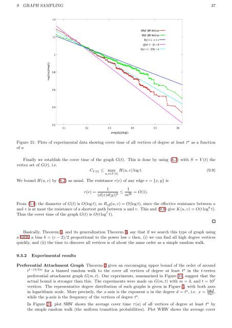
9 GRAPH SAMPLING 37Figure 21: Plots of experimental data showing cover time of all vertices of degree at least t a as a functionof aFinally we establish the cover time of the graph G(t). This is done by using (6.3) with S = V (t) thevertex set of G(t), i.e.C V (t) ≤ max H(u, v) log t. (9.9)u,v∈V (t)We bound H(u, v) by (6.2) as usual. The resistance r(e) of any edge e = {x, y} isr(e) =1(d(x)d(y)) b ≤ 1 = O(1).m2b From (5.4) the diameter of G(t) is O(log t), so R eff (u, v) = O(log t), since the effective resistance between uand v is at most the resistance of a shortest path between u and v. This and (9.8) give K(u, v) = O(t log 6 t).Thus the cover time of the graph G(t) is O(t log 7 t).Basically, Theorem 2, and its generalization Theorem 3, say that if we search this type of graph usinga SRW a bias b = (c − 2)/2 proportional to the power law c then, (i) we can find all high degree verticesquickly, and (ii) the time to discover all vertices is of about the same order as a simple random walk.9.3.2 Experimental resultsPreferential Attachment Graph Theorem 2 gives an encouraging upper bound of the order of aroundt 1−(4/3)a for a biassed random walk to the cover all vertices of degree at least t a in the t-vertexpreferential attachment graph G(m, t). Our experiments, summarized in Figure 21, suggest that theactual bound is stronger than this. The experiments were made on G(m, t) with m = 3, and t = 10 7vertices. The representative degree distribution of such graphs is given in Figure 2, with both axesin logarithmic scale. More precisely, the x-axis is the exponent a in the degree d = t a , i.e. x = log dlog t ,while the y-axis is the frequency of the vertices of degree t a .In Figure 21, plot SRW shows the average cover time τ(a) of all vertices of degree at least t a bythe simple random walk (the uniform transition probabilities). Plot WRW shows the average cover