Upgrade Report - Department of Informatics - King's College London

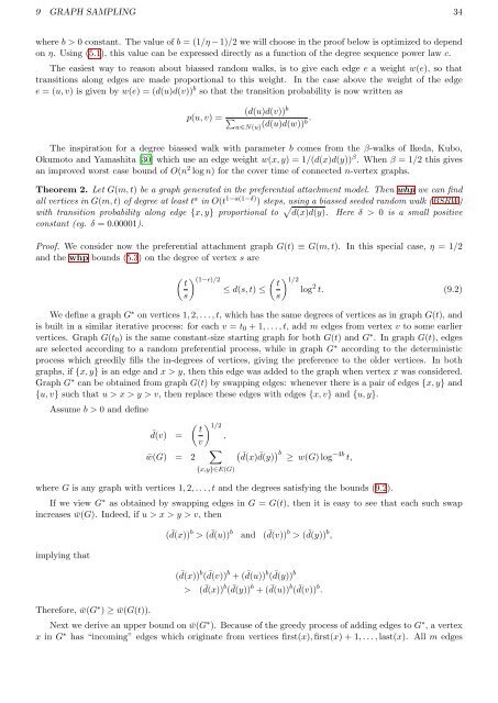
9 GRAPH SAMPLING 34where b > 0 constant. The value of b = (1/η − 1)/2 we will choose in the proof below is optimized to dependon η. Using (5.1), this value can be expressed directly as a function of the degree sequence power law c.The easiest way to reason about biassed random walks, is to give each edge e a weight w(e), so thattransitions along edges are made proportional to this weight. In the case above the weight of the edgee = (u, v) is given by w(e) = (d(u)d(v)) b so that the transition probability is now written asp(u, v) =(d(u)d(v)) b∑w∈N(u) (d(u)d(w))b .The inspiration for a degree biassed walk with parameter b comes from the β-walks of Ikeda, Kubo,Okumoto and Yamashita [30] which use an edge weight w(x, y) = 1/(d(x)d(y)) β . When β = 1/2 this givesan improved worst case bound of O(n 2 log n) for the cover time of connected n-vertex graphs.Theorem 2. Let G(m, t) be a graph generated in the preferential attachment model. Then whp we can findall vertices in G(m, t) of degree at least t a in O(t 1−a(1−δ) ) steps, using a biassed seeded random walk (BSRW)with transition probability along edge {x, y} proportional to √ d(x)d(y). Here δ > 0 is a small positiveconstant (eg. δ = 0.00001).Proof. We consider now the preferential attachment graph G(t) ≡ G(m, t). In this special case, η = 1/2and the whp bounds (5.3) on the degree of vertex s are) (1−ɛ)/2≤ d(s, t) ≤) 1/2log 2 t. (9.2)( ts( tsWe define a graph G ∗ on vertices 1, 2, . . . , t, which has the same degrees of vertices as in graph G(t), andis built in a similar iterative process: for each v = t 0 + 1, . . . , t, add m edges from vertex v to some earliervertices. Graph G(t 0 ) is the same constant-size starting graph for both G(t) and G ∗ . In graph G(t), edgesare selected according to a random preferential process, while in graph G ∗ according to the deterministicprocess which greedily fills the in-degrees of vertices, giving the preference to the older vertices. In bothgraphs, if {x, y} is an edge and x > y, then this edge was added to the graph when vertex x was considered.Graph G ∗ can be obtained from graph G(t) by swapping edges: whenever there is a pair of edges {x, y} and{u, v} such that u > x > y > v, then replace these edges with edges {x, v} and {u, y}.Assume b > 0 and define¯d(v) =¯w(G) = 2( tv) 1/2,∑{x,y}∈E(G)( ¯d(x) ¯d(y)) b ≥ w(G) log −4b t,where G is any graph with vertices 1, 2, . . . , t and the degrees satisfying the bounds (9.2).If we view G ∗ as obtained by swapping edges in G = G(t), then it is easy to see that each such swapincreases ¯w(G). Indeed, if u > x > y > v, thenimplying thatTherefore, ¯w(G ∗ ) ≥ ¯w(G(t)).( ¯d(x)) b > ( ¯d(u)) b and ( ¯d(v)) b > ( ¯d(y)) b ,( ¯d(x)) b ( ¯d(v)) b + ( ¯d(u)) b ( ¯d(y)) b> ( ¯d(x)) b ( ¯d(y)) b + ( ¯d(u)) b ( ¯d(v)) b .Next we derive an upper bound on ¯w(G ∗ ). Because of the greedy process of adding edges to G ∗ , a vertexx in G ∗ has “incoming” edges which originate from vertices first(x), first(x) + 1, . . . , last(x). All m edges