An Introduction to Error Correction Models An Introduction to ECMs ...

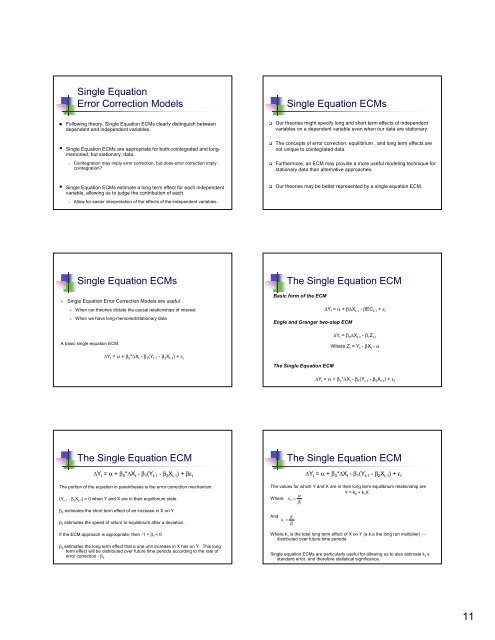
Single Equation
Error Correction Models
� Following theory, Single Equation ECMs clearly distinguish between
dependent and independent variables.
� Single Equation ECMs are appropriate for both cointegrated and longmemoried,
but stationary, data.
� Cointegration may imply error correction, but does error correction imply
cointegration?
� Single Equation ECMs estimate a long term effect for each independent
variable, allowing us to judge the contribution of each.
� Allow for easier interpretation of the effects of the independent variables.
Single Equation ECMs
� Single Equation Error Correction Models are useful
� When our theories dictate the causal relationships of interest
� When we have long-memoried/stationary data
A basic single equation ECM:
∆Y t = α + β 0 *∆X t - β 1 (Y t-1 - β 2 X t-1 ) + ε t
The Single Equation ECM
∆Y t = α + β 0*∆X t - β 1(Y t-1 - β 2X t-1) + βε t
The portion of the equation in parentheses is the error correction mechanism.
(Y t-1 - β 2 X t-1 ) = 0 when Y and X are in their equilibrium state
β 0 estimates the short term effect of an increase in X on Y
β 1 estimates the speed of return to equilibrium after a deviation.
If the ECM approach is appropriate, then -1 < β 1 < 0
β 2 estimates the long term effect that a one unit increase in X has on Y. This long
term effect will be distributed over future time periods according to the rate of
error correction - β 1
Single Equation ECMs
� Our theories might specify long and short term effects of independent
variables on a dependent variable even when our data are stationary.
� The concepts of error correction, equilibrium , and long term effects are
not unique to cointegrated data.
� Furthermore, an ECM may provide a more useful modeling technique for
stationary data than alternative approaches.
� Our theories may be better represented by a single equation ECM.
The Single Equation ECM
Basic form of the ECM
Engle and Granger two-step ECM
The Single Equation ECM
ΔY t = α + βΔX t-1 - βEC t-1 + ε t
∆Y t = β 0 ∆X t-1 - β 1 Z t-1
Where Z t = Y t - βX t - α
∆Y t = α + β 0 *∆X t - β 1 (Y t-1 - β 2 X t-1 ) + ε t
The Single Equation ECM
∆Y t = α + β 0*∆X t - β 1(Y t-1 - β 2X t-1) + ε t
The values for which Y and X are in their long term equilibrium relationship are
Y = k0 + k1X α
Where k0
=
β
And β 2
k1
=
β
1
1
Where k 1 is the total long term effect of X on Y (a.k.a the long run multiplier) - -
distributed over future time periods.
Single equation ECMs are particularly useful for allowing us to also estimate k 1 ’s
standard error, and therefore statistical significance.
11