A model of the wind-driven ocean circulation Version 1.0

A model of the wind-driven ocean circulation
Version 1.0
André Paul
February 15, 2006
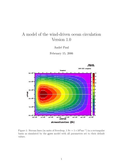
Figure 1: Stream lines (in units of Sverdrup, 1 Sv = 1×10 6 ms −1 ) in a rectangular
basin as simulated by the gyre model with all parameters set to their default
values.
1

1 System requirements
To run this ocean model and view its output on your Windows PC requires the
following software packages to be installed:
• cygwin (http://cygwin.com/)
• netCDF (http://www.unidata.ucar.edu/software/netcdf/)
• GMT (the ‘Generic Mapping Tools’, http://gmt.soest.hawaii.edu/)
• GSview (http://www.cs.wisc.edu/~ghost/gsview/packages)
• Ferret (http://ferret.pmel.noaa.gov/Ferret/)
2 How to get started
2.1 How to install the model
• Using Windows, download the ZIP-compressed folder gyre.zip from
http://www.palmod.uni-bremen.de/~apau/
• Do not open this folder, but save it, e.g. to the folder My Documents (Eigene
Dateien) on the desktop of your PC.
• Either right-click on the gyre.zip icon and extract all files directly to the
folder My Documents, or use any other tool to extract all files from this
ZIP-compressed folder.
2.2 Directory structure
The gyre directory contains the following subdirectories (in the UNIX/LINUX
world the term ‘directory’ is used for ‘folder’):
doc
gmt
input
output
src
tmp
work
documentation
GMT scripts *.gmt for plotting
input parameters *.in
model output *.dat or *.nc
Fortran 90 source code *.f90, if available
temporary subdirectory for compiling and plotting
executable program and (possibly) compile scripts
2

2.3 How to run the model
To ‘run’ (execute) the model, double-click on the start cygwin.bat icon in the
work directory. A cygwin window will appear. Type gyre.exe (or ./gyre.exe)
on the command line and press return. The model will start, print the current
values of the model parameters beta, taur and tau0 to the screen, run for a
few seconds, print out the number of iterations n it took to reach an equilibrium
solution and finish.
2.4 List of some useful UNIX/LINUX commands
ls
cd
cd ..
cp file1 file2
rm file
man command
pwd
gv or ggv
g95 or ifort
list directory contents
change directory to directory
change directory one level up
copy files and directories
remove file(s) or directories
format and display the on-line manual pages
print name of current/working directory
display ps files (may work for eps or pdf files as well)
compile Fortran 90 source file
2.5 Some LINUX hints
• Use the tab key to complete a command.
• Use the up and down keys to scroll through the history of previous coomands.
• To put ghostview (gv or ggv) or any editor (e.g. emacs) in the background,
add ‘ &’ at the end of the command line.
2.6 How to view the results
After running the gyre model, the output directory contains the following files:
snapshot.dat in human-readable ASCII format, snapshot.nc in binary netCDF
format. Both files contain the equilibrium solution for the wind-driven ocean
circulation in terms of a horizontal streamfunction. The contents of the file
snapshot.dat can be visualized using, e.g. ‘GMT’ (the ‘Generic Mapping Tools’,
http://gmt.soest.hawaii.edu/) - see the GMT script gyre.gmt in the gmt directory.
The contents of the file snapshot.nc can be visualized using, e.g. ‘ferret’:
3

• If you use a ‘German-language’ Windows operating system, open the file
init ferret.txt, turn those lines that refer to the ‘English-language’ Windows
operating system into comments, and activate those lines that refer
to the ‘German-language’ Windows operating system.
• Double-click on the start ferret.bat icon in the output directory to automatically
start up ‘ferret’ in this directory. A new cygwin window will
appear.
– To start ‘ferret’, now type: ferret.
– To load the output file into ‘ferret’, type: use snapshot.nc
– To check what data was loaded, type: show data
– To get a first idea of the model result, type: shade psi
If the shade psi command fails, close ‘ferret’ (by typing exit), start the
‘X windows server’ (by typing startx & in a different cygwin window),
then re-open ‘ferret’ (by typing ferret again).
If executing the start ferret.bat file fails, start up ‘ferret’ by executing the
ferret batch file from the ‘Start - All Programs’ menu. Find out where you are
by typing pwd and pressing ‘enter’. If you are not in the output directory, change
to it using the following sequence of commands:
cd c:
cd Documents and Settings
cd geo
cd Mydocuments
cd gyre
cd gyre
cd output
2.7 Further ‘ferret’ commands
show data
shade psi
cont psi
fill psi
plot/y=2500000 psi
list the loaded data
color-shade streamfunction
draw contour lines
draw color-filled contour lines
for a given value of y = 2500 km,
plot the streamfunction as a function of x
To compare the contents of two output files snapshot1.nc and snapshot2.nc,
use the following sequence of commands:
4

use snapshot1.nc
use snapshot2.nc
show data
fill psi[d=1]
fill psi[d=2]
plot/y=2500000 psi[d=1]
plot/y=2500000/overlay psi[d=2]
2.8 How to continue
To carry out a second experiment and compare the result to the first one, proceed
as follows:
• rename the output file snapshot.nc in the output directory to prevent
overwriting (e.g. type mv snapshot.nc snapshot1.nc in the cygwin window)
• change parameter(s) in the file input/gyre.in using the ‘Editor’, ‘Word-
Pad’ or notepad, save the file
• rerun the program work/gyre.exe, check the parameters read in (a new
output file is generated)
• rename the output file snapshot.nc in the output directory (e.g. type mv
snapshot.nc snapshot2.nc in the cygwin window)
• load output files into ‘ferret’ (e.g. type use snapshot1.nc in the ‘ferret’
window)
3 Model description
3.1 Model parameters
There are three key parameters that can be changed in the file input/gyre.in:
• beta (or β): rate of change of the Coriolis parameter with latitude (default
value: 2 × 10 −11 m −1 s −1 )
• taur (or τ r ): relaxation time scale for bottom (Rayleigh) friction (default
value: 6 days)
• tau0 (or τ 0 ): amplitude of zonal wind forcing (default value: 0.1 N m −2 )
5

The bottom (Rayleigh) friction parameter is given by R = 1/τ r . The relaxation
time scale τ r characterizes the time it would take for the circulation to slow down
if all other forcings could be ‘turned off’. The longer this timescale, the smaller
the friction.
A theoretical description of this model can be found in Stommel (1948), Open
University Course Team (1989, Section 4.2) and Mellor (1996, Section 6.3) - see
also Munk (1950) and Munk and Carrier (1952).
References
Mellor, G. L. (1996). Introduction to Physical Oceanography. Woodbury, New
York: American Institute of Physics.
Munk, W. H. (1950). On the wind-driven ocean circulation. Journal of Meteorology
7, 79–93.
Munk, W. H. and G. F. Carrier (1952). The wind-driven ocean circulation in
ocean basins of various shapes. Tellus 2, 158–167.
Open University Course Team (1989). Ocean Circulation. Milton Keynes:
Open University.
Stommel, H. (1948). The westward intensification of wind-driven ocean currents.
Transactions of the American Geophysical Union 29, 202–206.
6