Simple Linear Theory - UCLA Physics & Astronomy

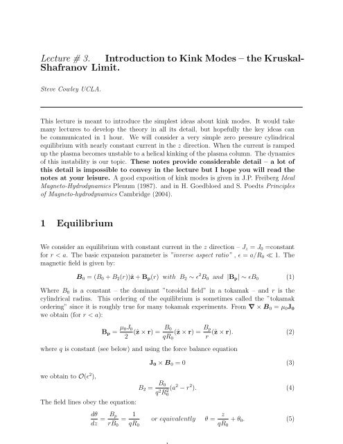
Lecture # 3. Introduction to Kink Modes – the Kruskal-
Shafranov Limit.
Steve Cowley UCLA.
This lecture is meant to introduce the simplest ideas about kink modes. It would take
many lectures to develop the theory in all its detail, but hopefully the key ideas can
be communicated in 1 hour. We will consider a very simple zero pressure cylindrical
equilibrium with nearly constant current in the z direction. When the current is ramped
up the plasma becomes unstable to a helical kinking of the plasma column. The dynamics
of this instability is our topic. These notes provide considerable detail – a lot of
this detail is impossible to convey in the lecture but I hope you will read the
notes at your leisure. A good exposition of kink modes is given in J.P. Freiberg Ideal
Magneto-Hydrodynamics Plenum (1987). and in H. Goedbloed and S. Poedts Principles
of Magneto-hydrodynamics Cambridge (2004).
1 Equilibrium
We consider an equilibrium with constant current in the z direction – J z = J 0 =constant
for r < a. The basic expansion parameter is ”inverse aspect ratio” , ɛ = a/R 0 ≪ 1. The
magnetic field is given by:
B 0 = (B 0 + B 2 (r))ẑ + B p (r) with B 2 ∼ ɛ 2 B 0 and |B p | ∼ ɛB 0 (1)
Where B 0 is a constant – the dominant ”toroidal field” in a tokamak – and r is the
cylindrical radius. This ordering of the equilibrium is sometimes called the ”tokamak
ordering” since it is roughly true for many tokamak experiments. From ∇ × B 0 = µ 0 J 0
we obtain (for r < a):
B p = µ 0J 0
2 (ẑ × r) = B 0
(ẑ × r) = B p
(ẑ × r). (2)
qR 0 r
where q is constant (see below) and using the force balance equation
we obtain to O(ɛ 2 ),
The field lines obey the equation:
J 0 × B 0 = 0 (3)
B 2 = B 0
(a 2 − r 2 ). (4)
q 2 R0
2
dθ
dz = B p
rB 0
= 1
qR 0
or equivalently θ = z
qR 0
+ θ 0 . (5)

2πR 0
a
b
Figure 1: Cylindrical Screw-pinch The plasma is contained in the region r < a and
the wall at r = b is considered perfectly conducting. The region between r = a and r = b
is the vacuum region. In the model considered here the (black) field lines in the plasma
all have the same rotational transform. The blue line is the vacuum field at the wall. The
two ends of the pinch are identified – i.e. it is periodic in z.
Thus all the plasma field lines have the same ”twist” – every time we go from one end of
the cylinder to the other the plasma field lines go around 1/q times in the θ ”poloidal”
direction. In tokamaks q is called the ”safety factor.” In the Fig. (1) the q is 0.4. Clearly
the greater the current the smaller the q – an upper limit on the current is then a lower
limit on q.
In the vacuum region the current is, of course, zero and the magnetic field is:
B 0 = B 0 ẑ + B 0a 2
The vacuum field has a q profile q v (r) = qr 2 /a 2 .
qr 2 R 0
(ẑ × r). (6)

2 Plasma Perturbation
To investigate stability we imagine pushing the plasma a small distance away from its
equilibrium state. Does the plasma move further away from or return to its equilibrium
state We model the plasma dynamics with Ideal Magneto-hydrodynamics (MHD). The
magnetic field obeys: the frozen-in law
which when linearized yields:
∂B
∂t
= ∇ × (v × B) (7)
δB = ∇ × (ξ × B 0 ) = B 0 · ∇ξ − ξ · ∇B 0 − B 0 ∇ · ξ. (8)
where ξ is the displacement of the plasma (∂ξ/∂t = v). The perturbed J × B force
accelerates the displacement. Thus the momentum equation becomes:
ρ 0
∂ 2 ξ
∂t 2 = J 0 × δB + (∇ × δB) × B 0 = F(ξ). (9)
The plasma density ρ 0 is taken to be constant and the pressure is set to zero. If we were
doing this formally we would now expand the components of this equation and solve the
eigenvalue problem for the growth rate. However we can get to the answer quicker by
using our intuition to figure out a good first approximation to the unstable perturbation.
We shall look at helical perturbations that move the column. Simply compressing the
strong z (toroidal) field makes a stable compressional Alfvén wave. Thus we take the
displacement to be dominantly a rigid helical shift of the plasma column, i.e.
ξ 0 = ξ 0
[cos ( z )ˆx + sin ( z ]
)ŷ = ξ 0 ˆξ0 . (10)
R 0 R 0
Each poloidal (x, y) plane of the plasma is shifted without distortiona constant distance
ξ 0 .
The radial displacement is
ξ r0 = ξ 0 · ˆr = ξ 0 cos (θ − z R 0
) (11)
This is the usual way to write the cylindrical displacement. We often expand as helical
modes with displacements proportional to exp (imθ − in z R 0
) – here (clearly) we are
examining m = n = 1 modes.
The field and current perturbations from the rigid displacement are from Eq. (14), using
Eqs. (2) and (4):
δB 0 = B [
0
(1 − q)(ξ
qR 0 × ẑ) + 2ξ ]
0 · r
ẑ
0 qR 0
δJ 0 = B [
0 (2 − q + q 2 )(ξ
µ 0 q 2 R0
2 0 × ẑ) ] (12)

2πR 0
ξ
Figure 2: Helical m=1 n=1 Kink displacement Rigid displacement of each poloidal
plane of the plasma by displacement of the form given by Eq. (10).
The first term in he field perturbation comes from bending the z (toroidal) field. The
second term is from moving the varying part toroidal field (B 2 ). Thus the perturbed
force from this displacement is (using Eq. (9)) is given by F 0 = − B2 0
µ 0
(1 + q)ξ
qR0 2 0 – this
is a stabilizing force since it opposes the motion! This displacement is not quite right.
Outside the plasma the vacuum field is perturbed and produces a pressure on the outside
of the plasma – this pressure will vary in θ in the same way as the perturbation. We
must match the magnetic pressure just inside the plasma with the magnetic pressure just
outside the plasma by slightly compressing the plasma. Thus we need to add to our plasma
displacement a small compressive component whose magnitude will be determined by the
matching of pressures at the boundary. For this compressive perturbation to produce a
constant force on the plasma and match the pressure from the vacuum at the boundary
it must be quadratic in r and point in the direction of ξ 0 . Thus we set:
ξ 2 = α r2
ξ
2qR0
2 0 . (13)
We shall determine the constant α so that the magnetic pressures balance at the boundary.
α is O(1) so that the compressional displacement is small, ξ 2 ∼ O(ɛ 2 )ξ 0 . With this small
compressional displacement the perturbed field and current become:

δB = B [
0
(1 − q)(ξ
qR 0 × ẑ) + (2 − αq)ξ ]
0 · r
ẑ
0 qR 0
δJ = B [
0 (2 − qα − q + q 2 )(ξ
µ 0 q 2 R0
2 0 × ẑ) ]
(14)
We keep the perturbed z magnetic field to O(ɛ 2 ) and the perturbed poloidal field to O(ɛ)
since they contribute to the magnetic pressure and the forces at the same order. The
compression contributes through compressing the z (toroidal) field. After a little algebra
the momentum equation becomes:
∂ 2 ξ
ρ 0
0 = F(ξ) = − B2 0
(1 + q − α)ξ
∂t 2 µ 0 qR0
2 0 . (15)
3 Vacuum Perturbation
In the vacuum ∇ × δB = 0 so we set δB = ∇χ. From ∇ · δB = 0 we obtain ∇ 2 χ = 0.
Taking χ = ˆχ(r) sin (θ − z R 0
) we find:
1
r
(
d
dr
r dˆχ
dr
)
− ˆχ r 2 − ˆχ R 2 0
= 0 (16)
We can drop the third term on the left hand side of this equation to lowest order and
obtain:
χ = (C 1 r + C 2
r + O(ɛ2 )) sin (θ − z R 0
) (17)
Where C 1 and C 2 are constants to be determined. The perturbed vacuum field is:
δB v = (C 1 − C 2
r 2 ) sin (θ − z R 0
)ˆr + (C 1 r + C 2
r ) cos (θ − z R 0
)[ 1 r ẑ × ˆr − 1 R 0
ẑ] (18)
At the conducting wall (r = b) we can have no radial field thus C 2 = b 2 C 1 .

n
a
ξ r
ξ
Figure 3: Vacuum-Plasma Interface. The shift of the boundary by the displacement
– to the order we keep the displacement is just ξ 0 . The boundary is given by the line
r = a + ξ r and the unit vector normal to the boundary is n.
4 Matching at the Vacuum-Plasma Interface
The normal to the perturbed ”flux” surfaces (labeled by their original radius r 0 ) is in the
direction of the ∇r 0 = ∇(r − ξ r ). Then to the order we need:
n = ˆr − ∇ξ r (19)
To join the plasma and vacuum solutions we must satisfy two conditions: 1) no field
through the vacuum-plasma interface and, 2) magnetic pressure continuity across the
vacuum-plasma interface.
No Vacuum Field Through the Vacuum-Plasma Interface.
(B 0 + δB v ) · (ˆr − ∇ξ r ) = 0 → B 0 · ∇ξ r = δB v · ˆr (20)
Substituting into this expression we determine C 1 in terms of ξ 0 :
C 1 = ξ 0B 0
(1 − 1)
q
R 0 (1 − b2
a 2 )
(21)
Magnetic Pressure Continuity Across the Vacuum-Plasma Interface.
Force balance across the plasma boundary becomes the continuity of magnetic pressure.

Thus on the surface r = r 0 + ξ r we have:
B 2 plasma = B 2 vacuum (22)
Using Eq. (14) and a little algebra we find:
B 2 plasma = B 2 0 + a2 B 2 0
q 2 R 2 0
and from Eqs. (18) and (21) we obtain:
B 2 vacuum = B 2 0 + a2 B 2 0
q 2 R 2 0
− 2B2 0ξ r
qR 2 0
+ 2B2 0ξ r
(1 − α) (23)
qR0
2
⎡
⎣ 1 q − q(1 − 1 q
b2
(
)2
( b2
⎤
+ 1)
a 2 ⎦ (24)
− 1)
a 2
Equating these expressions we obtain α = [1 + 1 q − q(1 − 1 q
Eq. (15) we obtain:
b2
(
a
)2 2 +1)
( b2
a
2 −1)]
and substituting into
∂ 2 ξ
ρ 0
0 = F(ξ) = 2B2 ( b2 − 1)
0 a 2 q
∂t 2 µ 0 qR0
2 ( b2 − 1) (1 q − 1)ξ 0. (25)
a 2
Clearly we have a growing mode when 1 > q > a 2 /b 2 with growth rate,
γ = √ 2B2 ( b2 − 1)
0 a 2 q
µ 0 ρ 0 qR0
2 ( b2 − 1) (1 − 1). (26)
q
a 2
When we set the conducting wall to go to infinity we get the Kruskal-Shafranov limit for
stability:
q > 1 → Stable. (27)
This is a limit on the current, specifically we must have µ 0 J 0 < 2B 0 /R 0 to be stable.
Although the stability criterion is very simple all the regions and forces play a role in
this instability. Specifically note that the field line bending forces in the plasma – the
1 + q part of the right hand side of Eq. (15) – are stabilizing. The vacuum pressure is
destabilizing since where ξ r > 0 the magnetic pressure on the boundary has decreased.

This arises because the vacuum field decreases with distance from the axis (as 1/r). The
decrease in pressure on the boundary is balanced in the plasma by a reduced z field caused
by an expansion of the plasma (where the radial displacement is positive ξ r > 0) – this
corresponds to (α > 0). The magnetic pressure forces from the expansion/compression
inside the plasma are then destabilizing. When q < 1 these pressure forces exceed the
field line bending forces and the plasma is unstable. Thus this is an external kink releasing
energy in the vacuum field – indeed the vacuum field lines straighten.
When the wall is close there is a narrow region of instability which corresponds to having
the q = 1 radius in the vacuum region – i.e. q v (r 1 ) = 1 = qr 2 1/a 2 . When the wall is present
the flux trapped between the plasma and the wall cannot escape and makes the vacuum
field pressure less destabilizing.
5 Other Kink Modes
In Tokamaks kink modes are driven by both current and pressure (Professor Brennan
will describe the situation in some detail) and the plasma is not cylindrical. Although
the m = n = 1 is often the most visible mode number the poloidal (m) harmonics are
coupled and none of the modes are a pure poloidal harmonic. The external kinks that are
observed can be predominantly higher harmonics. Often what one sees is a mode with
m/n ∼ q edge – where q edge is the value of q at the edge of the plasma. It is instructive to
draw the kinked boundary for the m = 2 mode.
Figure 4: Helical m=2 n=1 Kink displacement Eliptical displacement of each flux
surface in the plasma by displacement of the form given by ξ r ∝ cos (2θ − z R 0
).

6 Problem
Vertical and Horizontal Stability. Tokamaks have to be stable to moving up/down
or side to side. This puts constraints on the coil arrangement next to the plasma. Lets
look at the stability of current filaments as a model of this situation. Consider 5 current
filaments (current flowing in the z direction):
• ”Plasma” Filament initially at x = y = 0 representing the plasma carrying
current I plasma
• 2 Horizontal ”Coils” at x = ±1, y = 0 carrying current I 0
• 2 Vertical ”Coils” at y = ±1, x = 0 carrying current −I 0
Let us imagine that the plasma and coil currents are fixed – i.e. they do not change during
any motion of the plasma.
1. Draw the configuration.
2. Calculate the force on the undisplaced plasma
3. Calculate the force on the ”plasma” when it is displaced by a distance δ horizontally.
4. Calculate the force on the ”plasma” when it is displaced by a distance δ vertically.
5. In which direction is it unstable What is the growth rate if the plasma has a mass
M
6. How could you stabilize this instability Discuss!