Macroeconomic Forecasting and Structural Change - CEIS
Macroeconomic Forecasting and Structural Change - CEIS
Macroeconomic Forecasting and Structural Change - CEIS

Create successful ePaper yourself
Turn your PDF publications into a flip-book with our unique Google optimized e-Paper software.
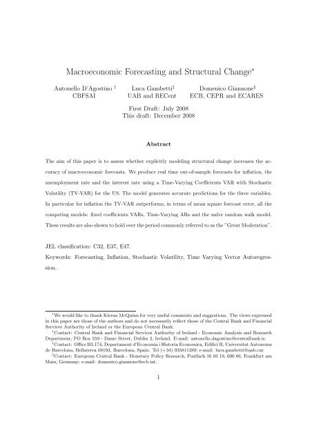
<strong>Macroeconomic</strong> <strong>Forecasting</strong> <strong>and</strong> <strong>Structural</strong> <strong>Change</strong> ∗<br />
Antonello D’Agostino †<br />
CBFSAI<br />
Luca Gambetti ‡<br />
UAB <strong>and</strong> RECent<br />
Domenico Giannone §<br />
ECB, CEPR <strong>and</strong> ECARES<br />
First Draft: July 2008<br />
This draft: December 2008<br />
Abstract<br />
The aim of this paper is to assess whether explicitly modeling structural change increases the accuracy<br />
of macroeconomic forecasts. We produce real time out-of-sample forecasts for inflation, the<br />
unemployment rate <strong>and</strong> the interest rate using a Time-Varying Coefficients VAR with Stochastic<br />
Volatility (TV-VAR) for the US. The model generates accurate predictions for the three variables.<br />
In particular for inflation the TV-VAR outperforms, in terms of mean square forecast error, all the<br />
competing models: fixed coefficients VARs, Time-Varying ARs <strong>and</strong> the naïve r<strong>and</strong>om walk model.<br />
These results are also shown to hold over the period commonly referred to as the ”Great Moderation”.<br />
JEL classification: C32, E37, E47.<br />
Keywords: <strong>Forecasting</strong>, Inflation, Stochastic Volatility, Time Varying Vector Autoregression.<br />
∗ We would like to thank Kieran McQuinn for very useful comments <strong>and</strong> suggestions. The views expressed<br />
in this paper are those of the authors <strong>and</strong> do not necessarily reflect those of the Central Bank <strong>and</strong> Financial<br />
Services Authority of Irel<strong>and</strong> or the European Central Bank.<br />
† Contact: Central Bank <strong>and</strong> Financial Services Authority of Irel<strong>and</strong> - Economic Analysis <strong>and</strong> Research<br />
Department, PO Box 559 - Dame Street, Dublin 2, Irel<strong>and</strong>. E-mail: antonello.dagostino@centralbank.ie.<br />
‡ Contact: Office B3.174, Departament d’Economia i Historia Economica, Edifici B, Universitat Autonoma<br />
de Barcelona, Bellaterra 08193, Barcelona, Spain. Tel (+34) 935811289; e-mail: luca.gambetti@uab.cat<br />
§ Contact: European Central Bank - Monetary Policy Research, Postfach 16 03 19, 600 66, Frankfurt am<br />
Main, Germany; e-mail: domenico.giannone@ecb.int.<br />
1
1 Introduction<br />
The US economy has undergone many structural changes during the post-WWII period.<br />
Long run trends in many macro variables have changed: average unemployment <strong>and</strong> inflation<br />
were particularly high during the 70s <strong>and</strong> low in the last decades (see Staiger, Stock,<br />
<strong>and</strong> Watson, 2001). Business cycle fluctuations have moderated substantially in the last<br />
twenty years <strong>and</strong> the volatility of output growth has reduced sharply. This latter phenomenon<br />
is typically referred to as the ”Great Moderation” (Stock <strong>and</strong> Watson, 2004).<br />
Also the dynamics of inflation have changed drastically: after the mid 80s inflation has<br />
become more stable <strong>and</strong> less persistent (see Cogley <strong>and</strong> Sargent, 2001). 1<br />
In addition to these series-specific changes many papers have documented important<br />
changes in the relationships between macroeconomic variables. For instance, some authors<br />
have argued that the Phillips curve is no longer a good characterization of the joint dynamics<br />
of inflation <strong>and</strong> unemployment. Such a claim is partly based on the result that the predictive<br />
content of unemployment for inflation has vanished since the mid 80s (Atkeson <strong>and</strong> Ohanian,<br />
2001; Roberts, 2006; Stock <strong>and</strong> Watson, 2008a). 2 The same period has seen significant<br />
changes in the conduct of macroeconomic policy. Foe example, according to many observers,<br />
monetary policy has become much more transparent <strong>and</strong> aggressive against inflation since<br />
the early 80s (Clarida, Gali, <strong>and</strong> Gertler, 2000).<br />
Given the relevance of macroeconomic changes, there are, surprisingly, few studies devoted<br />
to examining whether allowing for key structural changes can yield improvements in<br />
the forecast accuracy of traditional models. 3 This paper addresses this issue. Allowing for<br />
structural changes may improve the forecast performance for at least two reasons. First, it<br />
1 <strong>Change</strong>s in persistence are still debated, for instance Pivetta <strong>and</strong> Reis (2007) find that the changes are<br />
not significant.<br />
2 More generally, the ability to exploit macroeconomic linkages for predicting inflation <strong>and</strong> real activity<br />
seems to have declined remarkably since the mid-1980s, see D’Agostino, Giannone, <strong>and</strong> Surico (2006) <strong>and</strong><br />
Rossi <strong>and</strong> Sekhposyan (2008).<br />
3 Two notable exceptions are Doan, Litterman, <strong>and</strong> Sims (1984) <strong>and</strong> Stock <strong>and</strong> Watson (2007). The<br />
former is the first paper suggesting a potential important role for structural change in economic forecasting.<br />
The second studies the accuracy of inflation forecasts produced by a univariate unobservable component<br />
model with stochastic volatility.<br />
2
may allow us to capture <strong>and</strong> exploit changes in macroeconomic relationships. Such changes,<br />
besides the kinds of change described earlier, can also simply represent variations associated<br />
to different phases of the cycle due to some type of nonlinearities. 4 For instance Stock<br />
<strong>and</strong> Watson (2008b) suggest that the relationship implied by the Phillips curve is particularly<br />
observed during severe downturns. Second, empirical models that allow for structural<br />
changes can correctly detect <strong>and</strong> forecast changes in the long run dynamics, like the decline<br />
in trend inflation <strong>and</strong> unemployment observed since the mid 80s. This is particularly important<br />
since some authors have recently argued that variations in the persistent component<br />
can hide unchanged short term relationships among macroeconomic variables. For instance,<br />
Cogley, Primiceri, <strong>and</strong> Sargent (2008) find that the Phillips curve is reestablished once the<br />
trend component of inflation is correctly estimated.<br />
The model we use in this paper is sufficiently general <strong>and</strong> flexible to allow for all the kinds<br />
of structural change previously discussed. In particular, we use the Time-Varying Coefficients<br />
VAR with Stochastic Volatility (TV-VAR henceforth) as specified by Primiceri (2005).<br />
The model allows for a) changes in the predictable component (time-varying coefficients),<br />
which can be due to variations in the structural dynamic interrelations among macroeconomic<br />
variables; <strong>and</strong> b) changes in the unpredictable component (stochastic volatility), that<br />
is, variations in the size <strong>and</strong> correlation among forecast errors which can be due to changes<br />
in the size of exogenous shocks or their impact on macroeconomic variables. 5<br />
We forecast three macroeconomic variables for the US economy: the unemployment rate,<br />
inflation <strong>and</strong> a short term interest rate. Data are in real time <strong>and</strong> forecasts are computed<br />
using only the data that were available at the time the forecasts are made. This aims to<br />
mimic as close as possible the conditions faced by a forecaster in real-time. We compare<br />
the accuracy of the predictions (the mean square forecast errors) of the TV-VAR to that of<br />
other st<strong>and</strong>ard forecasting models: fixed coefficients VARs (estimated recursively or with<br />
rolling window), Time-Varying ARs <strong>and</strong> the naïve r<strong>and</strong>om walk model. We believe that the<br />
4 See Granger (2008).<br />
5 Allowing for the two sources of change is also important in the light of the ongoing debate about the<br />
relative importance of changes in the predictable <strong>and</strong> unpredictable components in the Great Moderation<br />
(Giannone, Lenza, <strong>and</strong> Reichlin, 2008).<br />
3
out-of-sample exercise is very informative concerning the forecasting potential of the TV-<br />
VAR. The reason is that the resulting mean square forecast error reflects both parameters<br />
uncertainty <strong>and</strong> model miss-specification. On the one h<strong>and</strong> the model is very flexible <strong>and</strong><br />
general, but, on the other h<strong>and</strong>, requires a large number of parameters to be estimated,<br />
<strong>and</strong> this might, in principle, introduce a large estimation uncertainty which may affect the<br />
reliability of the model for forecasting. In addition, the out-of-sample exercise will also<br />
provide indications on some subjective choices that are required for the estimation of the<br />
TV-VAR model, such as the setting of the prior beliefs on the relative amount of time<br />
variations in the coefficients.<br />
Our findings show that the TV-VAR is the only model which systematically delivers accurate<br />
forecasts for the three variables. For inflation the forecasts generated by the TV-VAR<br />
are much more accurate than those obtained with any other model. For unemployment, the<br />
forecasting accuracy of the TV-VAR model is very similar to that of the fixed coefficient<br />
VAR, while forecasts for the interest rate are comparable to that of the Time-Varying AR.<br />
These results hold for different sub-samples. In particular, they are also confirmed over<br />
the Great Moderation period, a period in which forecasting models are often found to have<br />
difficulties in outperforming simple naïve models in forecasting many macroeconomic variables<br />
(D’Agostino, Giannone, <strong>and</strong> Surico, 2006) <strong>and</strong>, in particular, inflation (Atkeson <strong>and</strong><br />
Ohanian, 2001). Results suggest that, on the one h<strong>and</strong> time varying models are “quicker”<br />
in recognizing structural changes in the permanent components of inflation <strong>and</strong> interest<br />
rate, <strong>and</strong>, on the other h<strong>and</strong>, that short term relationships among macroeconomic variables<br />
carry out important information, once structural changes are properly taken into account.<br />
The rest of the paper is organized as follows, section 2 describes the TV-VAR model;<br />
section 3 explains the forecasting exercise; section 4 presents the results <strong>and</strong> section 5<br />
concludes.<br />
2 The Time-Varying Vector Autoregressive Model<br />
In setting up our forecast exercise, let y t = (π t , UR t , IR t ) ′ where π t is the inflation rate,<br />
UR t the unemployment rate <strong>and</strong> IR t a short term interest rate. We assume that y t admits<br />
4
the following time varying coefficients VAR representation:<br />
y t = A 0,t + A 1,t y t−1 + ... + A p,t y t−p + ε t (1)<br />
where A 0,t contains time-varying intercepts, A i,t are matrices of time-varying coefficients,<br />
i = 1, ..., p <strong>and</strong> ε t is a Gaussian white noise with zero mean <strong>and</strong> time-varying covariance<br />
matrix Σ t . Let A t = [A 0,t , A 1,t ..., A p,t ], <strong>and</strong> θ t = vec(A ′ t), where vec(·) is the column stacking<br />
operator. Conditional on such an assumption, we postulate the following law of motion for<br />
θ t :<br />
θ t = θ t−1 + ω t (2)<br />
where ω t is a Gaussian white noise with zero mean <strong>and</strong> covariance Ω. We let Σ t = F t D t F ′ t,<br />
where F t is lower triangular, with ones on the main diagonal, <strong>and</strong> D t a diagonal matrix. Let<br />
σ t be the vector of the diagonal elements of D 1/2<br />
t<br />
<strong>and</strong> φ i,t , i = 1, ..., n −1 the column vector<br />
formed by the non-zero <strong>and</strong> non-one elements of the (i+1)-th row of Ft<br />
−1 . We assume that<br />
the st<strong>and</strong>ard deviations, σ t , evolve as geometric r<strong>and</strong>om walks, belonging to the class of<br />
models known as stochastic volatility. The simultaneous relations φ it in each equation of<br />
the VAR are assumed to evolve as independent r<strong>and</strong>om walks.<br />
log σ t = log σ t−1 + ξ t (3)<br />
φ i,t = φ i,t−1 + ψ i,t (4)<br />
where ξ t <strong>and</strong> ψ i,t are Gaussian white noises with zero mean <strong>and</strong> covariance matrix Ξ <strong>and</strong><br />
Ψ i , respectively. Let φ t = [φ ′ 1,t , . . .,φ′ n−1,t ], ψ t = [ψ 1,t ′ , . . .,ψ′ n−1,t ], <strong>and</strong> Ψ be the covariance<br />
matrix of ψ t . We assume that ψ i,t is independent of ψ j,t , for j ≠ i, <strong>and</strong> that ξ t , ψ t , ω t , ε t<br />
are mutually uncorrelated at all leads <strong>and</strong> lags. 6<br />
2.1 Forecasts<br />
Equation (1) has the following companion form<br />
y t = µ t + A t y t−1 + ǫ t<br />
6 In principle, one could make ε t <strong>and</strong> ω t correlated. However, it is well known that such model can be<br />
equivalently represented with a setup where shocks are mutually uncorrelated but ε t is serially correlated.<br />
Since our measurement equation is a VAR, such a flexibility is unneeded here.<br />
5
where y t = [y ′ t...y ′ t−p+1 ]′ , ǫ t = [ε ′ t0...0] ′ <strong>and</strong> µ t = [A ′ 0,t 0...0]′ are np × 1 vectors <strong>and</strong><br />
(<br />
)<br />
A t<br />
A t =<br />
I n(p−1) 0 n(p−1),n<br />
where A t = [A 1,t ...A p,t ] is an n ×np matrix, I n(p−1) is an n(p −1) ×n(p −1) identity matrix<br />
<strong>and</strong> 0 n(p−1),n is a n(p −1) ×n matrix of zeros. Let ˆµ t <strong>and</strong> Ât denote the median of the joint<br />
posterior distribution of ˆµ t  t (see appendix for the details). The forecast of y t+1 1-step<br />
ahead is:<br />
ŷ t+1|t = ˆµ t + Âty t (5)<br />
A technical issue arises when we generate multi-step expectations; we have to evaluate<br />
the future path of drifting parameters. We follow the literature <strong>and</strong> treat those parameters<br />
as if they had remained constant at the current level. 7 As a consequence, forecasts at time<br />
t + h are computed iteratively:<br />
2.2 Priors specification<br />
ŷ t+h|t = ˆµ t + Âtŷ t+h−1 =<br />
h∑<br />
j=1<br />
 j−1<br />
t ˆµ t + Âh t y t (6)<br />
We estimate the model using bayesian methods. While the details of the estimation in<br />
the Appendix, in this section we briefly discuss the specification of our priors. Following<br />
Primiceri (2005), we make the following assumptions for the priors densities. First, the<br />
coefficients of the covariances of the log volatilities <strong>and</strong> the hyperparameters are assumed<br />
to be independent of each other. The priors for the initial states θ 0 of the time varying<br />
coefficients, simultaneous relations φ 0 <strong>and</strong> log st<strong>and</strong>ard errors log σ are assumed to be<br />
normally distributed. The priors for the hyperparameters, Ω, Ξ <strong>and</strong> Ψ are assumed to be<br />
distributed as independent inverse-Wishart. More precisely, we have the following priors:<br />
• Time varying coefficients: P(θ 0 ) = N(ˆθ, ˆV θ ) <strong>and</strong> P(Ω) = IW(Ω −1<br />
0 , ρ 1);<br />
• Simultaneous relations: P(log σ 0 ) = N(log ˆσ, I n ) <strong>and</strong> P(Ψ i ) = IW(Ψ −1<br />
0i , ρ 3i);<br />
• Stochastic Volatilities: P(φ i0 ) = N(ˆφ i , ˆV φi ) <strong>and</strong> P(Ξ) = IW(Ξ −1<br />
0 , ρ 2);<br />
7 See Sbordone <strong>and</strong> Cogley (2008) for a discussion of the implications of this simplifying assumption.<br />
6
where the scale matrices are parametrized as follows Ω −1<br />
0 = λ 1 ρ 1 ˆVθ , Ψ 0i = λ 3i ρ 3i ˆVφi <strong>and</strong><br />
Ξ 0 = λ 2 ρ 2 I n . The hyper-parameters are calibrated using a time invariant recursive VAR<br />
estimated using a pre-sample consisting of the first T 0 observations. 8 For the initial states<br />
θ 0 <strong>and</strong> the contemporaneous relations φ i0 , we set the means, ˆθ <strong>and</strong> ˆφ i , <strong>and</strong> the variances, ˆV θ<br />
<strong>and</strong> ˆV φi , to be the maximum likelihood point estimates <strong>and</strong> four times its variance. For the<br />
initial states of the log volatilities, log σ 0 , the mean of the distribution is chosen to be the<br />
logarithm of the point estimates of the st<strong>and</strong>ard errors of the residuals of the estimated time<br />
invariant VAR. The degrees of freedom for the covariance matrix of the drifting coefficient’s<br />
innovations are set to be equal to T 0 , the size of the pre-sample. The degrees of freedom for<br />
the priors on the covariance of the stochastic volatilities’ innovations, are set to be equal to<br />
the minimum necessary for insuring the prior is proper. In particular, ρ 1 <strong>and</strong> ρ 2 are equal<br />
to the number of rows Ξ −1<br />
0 <strong>and</strong> Ψ −1<br />
0i<br />
plus one respectively. The parameters λ i are very<br />
important since they control the degree of time variations in the unobserved states. The<br />
smaller such parameters are, the smoother <strong>and</strong> smaller are the changes in coefficients. The<br />
empirical literature has set the prior to be rather conservative in terms of the amount of<br />
time variations. The exact parameterizations used will be discussed in the empirical section.<br />
3 Real-time forecasting<br />
Our objective is to predict the h-period ahead unemployment rate UR t+h , the interest<br />
rate IR t+h <strong>and</strong> the annualized price inflation πt+h h = 400<br />
h log(P t+h), where P t+h is the GDP<br />
deflator at time t + h <strong>and</strong> 400<br />
h<br />
is the normalization term.<br />
P t<br />
3.1 Data<br />
Prices are measured by the GDP deflator <strong>and</strong> the interest rate is measured by the three<br />
month treasury bills. We use real time databases for P t <strong>and</strong> UR t . 9 For the three month<br />
8 T 0 is equal to 32 quarters.<br />
9 The data are available on the Federal Reserve Bank of Philadelphia website at:<br />
http://www.phil.frb.org/econ/forecast/reaindex.html.<br />
7
interest rate we use the actual series. 10 Since unemployment <strong>and</strong> interest rate series are<br />
monthly, we follow Cogley <strong>and</strong> Sargent (2001, 2005) <strong>and</strong> Cogley, Primiceri, <strong>and</strong> Sargent<br />
(2008) <strong>and</strong> convert them into quarterly series by taking the middle month <strong>and</strong> the first<br />
month values in each quarter, respectively for UR t <strong>and</strong> IR t . We use quarterly vintages<br />
from 1969:Q4 to 2007:Q4. Vintages can differ since new data on the most recent period<br />
are released, but also because old data get revised. As a convention we date a vintage<br />
as the last quarter for which all data are available. For each vintage the sample starts<br />
in 1948:Q1. 11 For the GDP deflator we compute the annualized quarterly inflation rate,<br />
π t = 400 log( Pt<br />
P t−1<br />
). We perform an out-of-sample simulation exercise. 12<br />
The procedure<br />
consists of generating the forecasts by using the same information that would have been<br />
available to the econometrician who had produced the forecasts in real time. The simulation<br />
exercise begins in 1969:Q4 <strong>and</strong>, for such a vintage, parameters are estimated using the<br />
sample 1948:Q1 to 1969:Q4. 13 We compute the forecasts up to 12 quarters ahead outside<br />
the estimation window, from 1970:Q1 to 1972:Q4, <strong>and</strong> the results are stored. 14 Then, we<br />
move one quarter ahead <strong>and</strong> re-estimate the model using the data in vintage 1970:Q1.<br />
Forecasts from 1970:Q2 to 1973:Q1 are again computed <strong>and</strong> stored. This procedure is then<br />
repeated using all the available vintages. Predictions are compared with ex-post realized<br />
data vintages. Since data are continuously revised at each quarter, several vintages are<br />
available. Following Romer <strong>and</strong> Romer (2000) we compare with the figures published after<br />
the next two subsequent quarters.<br />
Two important aspects of the TV-VAR specification are worth noting. The first one<br />
concerns the setting of λ i , the parameter which fixes the tightness of the variance of the<br />
coefficients . In general, the literature has been quite conservative; very little time variation<br />
10 The series is available on the FRED dataset of the Federal Reserve Bank of St. Louis (mnemonics<br />
TB3MS), at: http://research.stlouisfed.org/fred2/series/TB3MS<br />
11 The vintages have a different time length, for example the sample span for the first vintage is 1948:Q1-<br />
1969:Q4, while the sample span for the last available vintage is 1948:Q1-2007:Q4.<br />
12 Because of revisions, data for the same period can differ across vintages. However, for notational<br />
simplicity we drop the indication of the vintage.<br />
13 The model is estimated with two lags.<br />
14 In the simulation exercise forecasts for horizon h = 1 correspond to nowcast, given that in real time<br />
data are available only up to the previous quarter.<br />
8
has been used in practice to set this parameter. The second aspect concerns the inclusion (or<br />
exclusion) of explosive draws from the analysis. That is, whether to keep or discard draws<br />
whose (VAR polynomial) roots lie inside the unit circle. We report results for the most<br />
conservative priors of Primiceri (2005) (λ 1 = .01, λ 2 = .1 <strong>and</strong> λ 3 = .01) <strong>and</strong> discard the<br />
explosive draws. However, we also run some robustness checks to underst<strong>and</strong> the sensitivity<br />
of the model to alternative specifications. In a first simulation, we set more stringent priors,<br />
while in a second simulation we keep the explosive draws.<br />
3.2 Other forecasting models<br />
We compare the forecast obtained with the TV-VAR with those obtained using different<br />
st<strong>and</strong>ard forecasting models. First, we consider Time Varying Autoregressions (TV-AR)<br />
for each for the three series. We will keep the same specification <strong>and</strong> prior beliefs used for<br />
the TV-VAR. Second, we also consider univariate (AR) <strong>and</strong> multivariate (VAR) forecasts<br />
produced using fixed coefficient models 15 . The models are estimated either recursively<br />
(REC), i.e. using all the data available at the time the forecast are made or using a rolling<br />
(ROL) window, i.e using the most recent ten years of data available at the time the forecast<br />
are made. The estimation over a rolling window is a very simple device to take time<br />
variation into account. The forecasts computed using the recursive <strong>and</strong> rolling window (on<br />
the VAR <strong>and</strong> AR models) will be denoted by VAR-REC, VAR-ROL, AR-REC, <strong>and</strong> AR-<br />
ROL respectively for the two models. Notice that the models predict quarterly inflation,<br />
therefore the forecasts for the h− quarter inflation πt+h h are computed by cumulating the<br />
first h forecasts of the first entries (which correspond to π t ) of the forecasted vector ŷ t+h|t ,<br />
that is ˆπ<br />
t+h|t h = 1 ∑ hi=1<br />
h ˆπ t+i|t .<br />
We will also compute no-change forecasts which are used as a benchmark. According to<br />
this naïve model, unemployment <strong>and</strong> interest rate next h− quarter ahead are predicted to be<br />
equal to the value observed in the current quarter. In the case of inflation we use a different<br />
benchmark. Atkeson <strong>and</strong> Ohanian (2001) demonstrated that, since 1984, structural models<br />
of US inflation have been outperformed by a naïve forecasts based on the average rate of<br />
inflation over the current <strong>and</strong> previous three quarters. This is essentially a ”no change”<br />
15 The models are estimated with two lags.<br />
9
forecast for annual inflation:<br />
ˆπ h,ao<br />
t+h|t = π4 t = 1 4 (π t + π t−1 + π t−2 + π t−3 ) (7)<br />
3.3 Forecast evaluation<br />
Forecast accuracy is evaluated by means of the Mean Square Forecast Error (MSFE). The<br />
MSFE is a measure of the average forecast accuracy over the out-of-sample window. In the<br />
empirical exercise we use two samples to evaluate forecasting accuracy. The full sample,<br />
1970 : Q1 −2007 : Q4 <strong>and</strong> the sample 1985 : Q1 −2007 : Q4. This latter period corresponds<br />
to the great moderation period. To facilitate the comparison between various models, the<br />
results are reported in terms of relative MSFE statistics, that is the ratio between the MSFE<br />
of a particular model to the MSFE of the naïve model, used as the benchmark. When the<br />
relative MSFE is less than one, forecasts produced with a given non-benchmark model are,<br />
on average, more accurate that those produced with the benchmark model. For example,<br />
a value of 0.8 indicates that the model under consideration improves upon the benchmark<br />
by 20%.<br />
4 Results<br />
This section discusses the main findings of the forecasting exercise. Table 2 summarizes the<br />
results of the real time forecast evaluation, over the whole sample, for the three variables<br />
(inflation rate π t , unemployment rate UR t <strong>and</strong> the interest rate IR t ), <strong>and</strong> for the forecast<br />
horizons of one quarter, one year, two years <strong>and</strong> three years ahead. For the benchmark<br />
naïve models we report the MSFE, while for the remaining models we report the MSFE<br />
relative to that of the naïve model (RMSFE). The overall performance of each model is<br />
summarized, at each horizon, by averaging over the three variables.<br />
Overall the TV-VAR produces very accurate forecasts for all the variables <strong>and</strong>, on<br />
average, performs better than any other model considered. In particular it outperforms<br />
the naïve benchmark for all the variables at all horizons with gains ranging from 5 to 28<br />
percent. As far as inflation is concerned, the TV-VAR model produces the best forecast with<br />
an average (over the horizons) improvements of about 30% relative to the benchmark. A<br />
10
elative good performance is also observed for the TV-AR with improvements of about 10%<br />
at horizons of 1 <strong>and</strong> 2 years. On the other h<strong>and</strong>, all the other time invariant specifications,<br />
univariate <strong>and</strong> multivariate, fail to improve upon the benchmark in terms of forecasting<br />
accuracy. For unemployment, the TV-VAR, together with the VAR-REC, is the model<br />
that delivers the most accurate predictions. For the three years, horizon the improvement<br />
relative to the naïve model is of about 52%. However, it is interesting to notice that,<br />
except for the AR-ROL, all the models display a good forecasting performance especially<br />
at long horizons. Finally, for the interest rate we find that, in general, the time varying<br />
specifications are those that perform better. In particular, the TV-VAR model delivers<br />
forecasts slightly more accurate than the TV-AR specification: at a three years horizon<br />
the two models improve the forecast accuracy of the naïve benchmark by 16% <strong>and</strong> 9%<br />
respectively.<br />
These findings show that time varying models are quicker than fixed parameters specifications<br />
to recognize structural changes in the permanent components of inflation <strong>and</strong><br />
interest rate. They also suggest that interrelations among macroeconomic variables carry<br />
out important information for forecasting, especially for unemployment <strong>and</strong> inflation, given<br />
that the accuracy of the multivariate time varying specification is always better than that<br />
of the univariate counterparts.<br />
Table 3 shows the results for the “Great Moderation” period. Such a period is particularly<br />
of interest because it has been shown that it is extremely difficult to produce forecasts<br />
which are more accurate than those obtained with simple naïve r<strong>and</strong>om walk models; however,<br />
also in this period, most of the earlier findings are confirmed. First, the TV-VAR<br />
model generates the most accurate forecasts for all the variables. Second, the TV-VAR<br />
is again the model producing the best forecast for inflation with an average improvement<br />
(over the horizons) of about 30% on the r<strong>and</strong>om walk. In particular, the model performs<br />
very well for long run inflation forecasts, the improvement at the 3 years horizon is almost<br />
double that of the full sample, it is now about 52%; therefore the predictability of inflation<br />
can be reestablished once time variations are accounted for. This seems to confirm the<br />
viewpoint of Cogley, Primiceri, <strong>and</strong> Sargent (2008) <strong>and</strong> Stock <strong>and</strong> Watson (2008b), who<br />
point out that the death of the Phillips curve is an artifact due to the neglected inflation<br />
11
trends <strong>and</strong> non-linearities. Third, forecasts of the interest rate obtained with the time<br />
varying models are more accurate than those in the previous sample. This might reflect<br />
the increased importance of the systematic predictable component of monetary policy in<br />
the last two decades. Finally, time varying methods also display more accurate forecasts,<br />
relative to the previous sample, for the unemployment rate series, over the longer horizons.<br />
Finally, Tables 4-7 report the results of two different forecast simulations over the two<br />
samples. In the first one we use a more stringent priors specification to generate the forecasts.<br />
By more stringent we mean that we assume an a priori smaller degree of variation in<br />
all the coefficients. Results are comparable, in terms of accuracy, with those obtained with<br />
the previous specification. The general message is that forecasts are particularly accurate<br />
when we attribute low probabilities of structural change. In the second simulation, we keep<br />
the explosive draws generated in the Gibb sampler algorithm. In this case the accuracy of<br />
the forecasts deteriorates for all the variables <strong>and</strong> in particular for the unemployment rate<br />
<strong>and</strong> interest rate. This result, we believe, is especially interesting since there is no clear<br />
consensus about whether explosive draws should be discarded or not. Here we provide a<br />
reason for ignoring explosive draws based on an out-of-sample forecast exercise.<br />
5 Conclusions<br />
The US economy has changed substantially during the post-WWII period. This paper tries<br />
to assess whether explicitly modeling these changes can improve the forecasting accuracy<br />
of key macroeconomic time series.<br />
We produce real time out-of sample forecasts for inflation, the unemployment rate <strong>and</strong><br />
a short term interest rate using time-varying coefficients VAR with stochastic volatility <strong>and</strong><br />
we compare its forecasting performance to that of other st<strong>and</strong>ard models: fixed coefficients<br />
VARs, Time-Varying ARs <strong>and</strong> the naïve r<strong>and</strong>om walk model. Our findings show that the<br />
TV-VAR is the only model which systematically delivers accurate forecasts for the three<br />
variables. For inflation, the forecasts generated by the TV-VAR are much more accurate<br />
than those obtained with any other model. These results hold for the Great Moderation<br />
period (the period since the mid 1980’s). On this sample, it is found that forecasting<br />
12
models have considerable difficulty in outperforming simple naïve models in predicting many<br />
macroeconomic variables <strong>and</strong>, in particular, inflation.<br />
Two main conclusions can be drawn. First, accounting for time variations <strong>and</strong> structural<br />
change is important for forecasting. Incorporating, in a flexible way, the features of a timevarying<br />
economy in the model substantially improves the forecast accuracy for the main<br />
macroeconomic variables. Second, the TV-VAR model turns out to be a very powerful<br />
tool for forecasting. Although it requires a relatively large number of parameters to be<br />
estimated, the gain in terms of generality <strong>and</strong> flexibility are very apparent.<br />
This is a first step in the investigation of how structural changes can be used for improving<br />
macroeconomic forecasting. Many interesting aspect remain to be investigated. First, it<br />
would be interesting to compare the results with other alternative fixed coefficients models.<br />
Second, it would be particularly useful to introduce forecast uncertainty in order to have<br />
some measure of dispersion of the point forecasts.<br />
13
References<br />
Atkeson, A., <strong>and</strong> L. E. Ohanian (2001): “Are Phillips Curves Useful for <strong>Forecasting</strong><br />
Inflation,” Quarterly Review, pp. 2–11.<br />
Carter, C. K., <strong>and</strong> R.Kohn (1994): “On Gibbs Sampling for State Space Models,”<br />
Biometrika, 81, 541–553.<br />
Clarida, R., J. Gali, <strong>and</strong> M. Gertler (2000): “Monetary Policy Rules And <strong>Macroeconomic</strong><br />
Stability: Evidence And Some Theory,” Quarterly Journal of Economics, 115(1),<br />
147–180.<br />
Cogley, T., G. E. Primiceri, <strong>and</strong> T. J. Sargent (2008): “Inflation-Gap Persistence<br />
in the U.S.,” NBER Working Paper 13749, NBER.<br />
Cogley, T., <strong>and</strong> T. J. Sargent (2001): “Evolving Post WWII U.S. Inflation Dynamics,”<br />
in <strong>Macroeconomic</strong>s Annual, pp. 331–373. MIT Press.<br />
(2005): “Drifts <strong>and</strong> Volatilities: Monetary Policies <strong>and</strong> Outcomes in the Post<br />
WWII US,” Review of Economic Dynamics, 8, 262–302.<br />
D’Agostino, A., D. Giannone, <strong>and</strong> P. Surico (2006): “(Un)Predictability <strong>and</strong> <strong>Macroeconomic</strong><br />
Stability,” Working Paper Series 605, European Central Bank.<br />
Doan, T., R. Litterman, <strong>and</strong> C. A. Sims (1984): “<strong>Forecasting</strong> <strong>and</strong> Conditional Projection<br />
Using Realistic Prior Distributions,” Econometric Reviews, 3, 1–100.<br />
Giannone, D., M. Lenza, <strong>and</strong> L. Reichlin (2008): “Explaining The Great Moderation:<br />
It Is Not The Shocks,” Journal of the European Economic Association, 6(2-3), 621 – 633.<br />
Granger, C. W. J. (2008): “Non-Linear Models: Where Do We Go Next-Time Varying<br />
Parameter Models,” Studies in Nonlinear Dynamics <strong>and</strong> Econometrics, 12.<br />
Pivetta, F., <strong>and</strong> R. Reis (2007): “The Persistence of Inflation in the United States,”<br />
Journal of Economic Dynamics <strong>and</strong> Control, 31, No.4, 1326–1358.<br />
14
Primiceri, G. E. (2005): “Time Varying <strong>Structural</strong> Vector Autoregressions <strong>and</strong> Monetary<br />
Policy,” Review of Economic Studies, 72, 821–852.<br />
Roberts, J. M. (2006): “Monetary Policy <strong>and</strong> Inflation Dynamics,” ijcb, 2(3), 193–230.<br />
Romer, David, H., <strong>and</strong> C. Romer (2000): “Federal Reserve Information <strong>and</strong> the Behavior<br />
of Interest Rates,” American Economic Review, 90, 429 – 457.<br />
Rossi, B., <strong>and</strong> T. Sekhposyan (2008): “as models forecasting performance for US output<br />
growth <strong>and</strong> inflation changed over time, <strong>and</strong> when,” Manuscript, Duke University.<br />
Sbordone, A. M., <strong>and</strong> T. Cogley (2008): “Trend Inflation <strong>and</strong> Inflation Persistence in<br />
the New Keynesian Phillips Curve,” American Economic Review, forthcoming.<br />
Staiger, D., J. H. Stock, <strong>and</strong> M. W. Watson (2001): “Prices, Wages, <strong>and</strong> the U.S.<br />
NAIRU in the 1990s,” in In The Roaring Nineties: Can Full Employment Be Sustained,<br />
ed. by A. B. Krueger, <strong>and</strong> R. M. Solow. Russell Sage Foundation.<br />
Stock, J. H., <strong>and</strong> M. W. Watson (2004): “Has the Business Cycle <strong>Change</strong>d <strong>and</strong> Why,”<br />
in NBER <strong>Macroeconomic</strong>s Annual 2003, ed. by M. Gertler, <strong>and</strong> K. Rogoff. MIT Press.<br />
(2007): “Why Has U.S. Inflation Become Harder to Forecast,” Journal of Money,<br />
Credit <strong>and</strong> Banking, 39, No.1.<br />
(2008a): “Phillips Curve Inflation Forecasts,” NBER Working Paper 14322, NBER.<br />
(2008b): “Phillips Curve Inflation Forecasts,” NBER Working Paper 2005-42,<br />
14322.<br />
15
Appendix<br />
Estimation is done using Bayesian methods. To draw from the joint posterior distribution of<br />
model parameters we use a Gibbs sampling algorithm along the lines described in Primiceri<br />
(2005). The basic idea of the algorithm is to draw sets of coefficients from known conditional<br />
posterior distributions. The algorithm is initialized at some values <strong>and</strong>, under some<br />
regularity conditions, the draws converge to a draw from the joint posterior after a burn in<br />
period. Let z be (q × 1) vector, we denote z T the sequence [z 1 ′ , ..., z′ T ]′ . Each repetition is<br />
composed of the following steps:<br />
1. p(σ T |x T , θ T , φ T , Ω, Ξ, Ψ, s T )<br />
2. p(s T |x T , θ T , σ T , φ T , Ω, Ξ, Ψ) 16<br />
3. p(φ T |x T , θ T , σ T , Ω, Ξ, Ψ, s T )<br />
4. p(θ T |x T , σ T , φ T , Ω, Ξ, Ψ, s T )<br />
5. p(Ω|x T , θ T , σ T , φ T , Ξ, Ψ, s T )<br />
6. p(Ξ|x T , θ T , σ T , φ T , Ω, Ψ, s T )<br />
7. p(Ψ|x T , θ T , σ T , φ T , Ω, Ξ, s T )<br />
Gibbs sampling algorithm<br />
• Step 1: sample from p(σ T |y T , θ T , φ T , Ω, Ξ, Ψ, s T )<br />
To draw σ T we use the algorithm of Kim, Shephard <strong>and</strong> Chibb (KSC) (1998). Consider<br />
the system of equations yt ∗ ≡ Ft −1 (y t − X tθ ′ t ) = D 1/2<br />
t u t , where u t ∼ N(0, I), X t = (I n ⊗ x ′ t),<br />
<strong>and</strong> x t = [1 n , y t−1 ...y t−p ]. Conditional on y T , θ T , <strong>and</strong> φ T , y ∗ t is observable. Squaring <strong>and</strong><br />
taking the logarithm, we obtain<br />
16 See below the definition of s T .<br />
y ∗∗<br />
t = 2r t + υ t (8)<br />
r t = r t−1 + ξ t (9)<br />
16
where y ∗∗<br />
i,t = log((y∗ i,t )2 +0.001) - the constant (0.001) is added to make estimation more robust<br />
- υ i,t = log(u 2 i,t ) <strong>and</strong> r t = log σ i,t . Since, the innovation in (8) is distributed as log χ 2 (1),<br />
we use, following KSC, a mixture of 7 normal densities with component probabilities q j ,<br />
means m j − 1.2704, <strong>and</strong> variances v 2 j<br />
(j=1,...,7) to transform the system in a Gaussian<br />
one, where {q j , m j , v 2 j } are chosen to match the moments of the log χ2 (1) distribution. The<br />
values are:<br />
Table 1: Parameters Specification<br />
j q j m j vj<br />
2<br />
1.0000 0.0073 -10.1300 5.7960<br />
2.0000 0.1056 -3.9728 2.6137<br />
3.0000 0.0000 -8.5669 5.1795<br />
4.0000 0.0440 2.7779 0.1674<br />
5.0000 0.3400 0.6194 0.6401<br />
6.0000 0.2457 1.7952 0.3402<br />
7.0000 0.2575 -1.0882 1.2626<br />
Let s T = [s 1 , ..., s T ] ′ be a matrix of indicators selecting the member of the mixture to<br />
be used for each element of υ t at each point in time. Conditional on s T , (υ i,t |s i,t = j) ∼<br />
N(m j − 1.2704, vj 2 ). Therefore we can use the algorithm of Carter <strong>and</strong> R.Kohn (1994) to<br />
draw r t (t=1,...,T) from N(r t|t+1 , R t|t+1 ), where r t|t+1 = E(r t |r t+1 , y t , θ T , φ T , Ω, Ξ, Ψ, s T , )<br />
<strong>and</strong> R t|t+1 = V ar(r t |r t+1 , y t , θ T , φ T , Ω, Ξ, Ψ, s T ).<br />
• Step 2: sample from p(s T |y T , θ T , σ T , φ T , Ω, Ξ, Ψ)<br />
Conditional on y ∗∗<br />
i,t <strong>and</strong> rT , we independently sample each s i,t from the discrete density<br />
defined by Pr(s i,t = j|y ∗∗<br />
i,t , r i,t) ∝ f N (y ∗∗<br />
i,t |2r i,t + m j − 1.2704, v 2 j ), where f N(y|µ, σ 2 ) denotes<br />
a normal density with mean µ <strong>and</strong> variance σ 2 .<br />
• Step 3: sample from p(φ T |y T , θ T , σ T , Ω, Ξ, Ψ, s T )<br />
Consider again the system of equations Ft<br />
−1 (y t − X tθ ′ t ) = Ft −1 ŷ t = D 1/2<br />
t u t . Conditional<br />
on θ T , ŷ t is observable. Since F −1<br />
t<br />
is lower triangular with ones in the main diagonal, each<br />
17
equation in the above system can be written as<br />
ŷ 1,t = σ 1,t u 1,t (10)<br />
ŷ i,t = −ŷ [1,i−1],t φ i,t + σ i,t u i,t i = 2, ..., n (11)<br />
where σ i,t <strong>and</strong> u i,t are the ith elements of σ t <strong>and</strong> u t respectively, ŷ [1,i−1],t = [ŷ 1,t , ...,ŷ i−1,t ].<br />
Under the block diagonality of Ψ, the algorithm of Carter <strong>and</strong> R.Kohn (1994) can be<br />
applied equation by equation, obtaining draws for φ i,t from a N(φ i,t|t+1 , Φ i,t|t+1 ), where<br />
φ i,t|t+1 = E(φ i,t |φ i,t+1 , y t , θ T , σ T , Ω, Ξ, Ψ) <strong>and</strong> Φ i,t|t+1 = V ar(φ i,t |φ i,t+1 , y t , θ T , σ T , Ω, Ξ, Ψ).<br />
• Step 4: sample from p(θ T |y T , σ T , φ T , Ω, Ξ, Ψ, s T )<br />
Conditional on all other parameters <strong>and</strong> the observables we have<br />
y t = X ′ tθ t + ε t (12)<br />
θ t = θ t−1 + ω t (13)<br />
Draws for θ t can be obtained from a N(θ t|t+1 , P t|t+1 ), where θ t|t+1 = E(θ t |θ t+1 , y T , σ T , φ T , Ω, Ξ, Ψ)<br />
<strong>and</strong> P t|t+1 = V ar(θ t |θ t+1 , y T , σ T , φ T , Ω, Ξ, Ψ) are obtained with the algorithm of Carter <strong>and</strong><br />
R.Kohn (1994).<br />
• Step 5: sample from p(Ω|y T , θ T , σ T , φ T , Ξ, Ψ, s T )<br />
Conditional on the other coefficients <strong>and</strong> the data, Ω has an Inverse-Wishart posterior<br />
density with scale matrix Ω −1<br />
1 = (Ω 0 + ∑ T<br />
t=1 ∆θ t (∆θ t ) ′ ) −1 <strong>and</strong> degrees of freedom df Ω1 =<br />
df Ω0 +T, where Ω −1<br />
0 is the prior scale matrix, df Ω0 are the prior degrees of freedom <strong>and</strong> T is<br />
length of the sample use for estimation. To draw a realization for Ω make df Ω1 independent<br />
draws z i (i=1,...,df Ω1 ) from N(0, Ω −1<br />
1 ) <strong>and</strong> compute Ω = (∑df Ω 1<br />
i=1 z iz ′ i )−1 (see Gelman et. al.,<br />
1995).<br />
• Step 6: sample from p(Ξ i,i |y T , θ T , σ T , φ T , Ω, Ψ, s T )<br />
Conditional the other coefficients <strong>and</strong> the data, Ξ has an Inverse-Wishart posterior<br />
density with scale matrix Ξ −1<br />
1 = (Ξ 0 + ∑ T<br />
t=1 ∆ log σ t (∆ log σ t ) ′ ) −1 <strong>and</strong> degrees of freedom<br />
df Ξ1 = df Ξ0 + T where Ξ −1<br />
0 is the prior scale matrix <strong>and</strong> df Ξ0 the prior degrees of freedom.<br />
Draws are obtained as in step 5.<br />
• Step 7: sample from p(Ψ|y T , θ T , σ T , φ T , Ω, Ξ, s T ).<br />
18
Conditional on the other coefficients <strong>and</strong> the data, Ψ i has an Inverse-Wishart posterior<br />
density with scale matrix Ψ −1<br />
i,1 = (Ψ i,0 + ∑ T<br />
t=1 ∆φ i,t (∆φ i,t ) ′ ) −1 <strong>and</strong> degrees of freedom<br />
df Ψi,1 = df Ψi,0 + T where Ψ −1<br />
i,0 is the prior scale matrix <strong>and</strong> df Ψ i,0<br />
the prior degrees of<br />
freedom. Draws are obtained as in step 5 for all i.<br />
19
Tables<br />
Table 2: <strong>Forecasting</strong> Accuracy over the sample: 1970-2007<br />
Horizons Series Naïve AR-REC AR-ROL TV-AR VAR-REC VAR-ROL TV-VAR<br />
(MSFE) (RMSFE) (RMSFE) (RMSFE) (RMSFE) (RMSFE) (RMSFE)<br />
π 2.15 1.13 1.08 1.03 1.15 1.01 0.86<br />
1 quarter UR 0.15 1.00 1.08 1.00 0.99 1.18 1.02<br />
IR 0.87 1.12 1.23 1.04 0.99 1.09 0.97<br />
Avg. 1.08 1.13 1.02 1.04 1.09 0.95<br />
π 2.24 1.17 1.03 0.88 1.37 1.22 0.62<br />
1 year UR 1.07 1.03 1.24 1.01 0.67 0.91 0.78<br />
IR 3.46 1.05 1.20 0.95 0.96 1.39 0.92<br />
Avg. 1.08 1.16 0.95 1.00 1.17 0.77<br />
π 3.06 1.19 1.13 0.93 1.6 1.38 0.66<br />
2 years UR 2.39 0.95 1.14 0.95 0.45 0.63 0.62<br />
IR 7.54 1.05 1.18 0.92 0.99 1.44 0.88<br />
Avg. 1.06 1.15 0.93 1.01 1.15 0.72<br />
π 3.31 1.28 1.24 1.00 1.93 1.60 0.72<br />
3 years UR 3.22 0.85 1.12 0.86 0.47 0.85 0.59<br />
IR 10.28 1.08 1.15 0.91 1.03 1.32 0.84<br />
Avg. 1.07 1.17 0.92 1.14 1.26 0.72<br />
First column, horizons; second column, series; third column MSFE of naïve models; other columns,<br />
relative MSFE, that is, ratio of the MSFE of a particular model to the MSFE of the naïve model. For<br />
each horizon is also reported the average of the relative MSFE across variables (Avg.).<br />
20
Table 3: <strong>Forecasting</strong> Accuracy over the sample: 1985-2007<br />
Horizons Series Naïve AR-REC AR-ROL TV-AR VAR-REC VAR-ROL TV-VAR<br />
(MSFE) (RMSFE) (RMSFE) (RMSFE) (RMSFE) (RMSFE) (RMSFE)<br />
π 20.93 2.61 1.19 1.21 1.29 1.35 0.98<br />
1 quarter UR 0.05 2.80 1.16 1.07 1.09 1.17 1.02<br />
IR 0.27 3.64 1.08 0.83 0.87 1.02 0.82<br />
Avg. 3.02 1.14 1.04 1.08 1.18 0.94<br />
π 0.45 5.76 1.54 1.16 2.22 2.64 0.91<br />
1 year UR 0.37 3.00 1.15 0.82 0.97 1.23 0.88<br />
IR 2.09 1.74 1.17 0.81 0.78 1.20 0.81<br />
Avg. 3.50 1.29 0.93 1.32 1.69 0.87<br />
π 0.57 6.39 2.09 1.08 3.03 3.11 0.77<br />
2 years UR 1.33 1.72 0.86 0.56 0.42 0.72 0.57<br />
IR 5.16 1.53 1.05 0.74 0.67 1.20 0.74<br />
Avg. 3.21 1.33 0.79 1.37 1.68 0.69<br />
π 0.92 4.61 2.10 0.86 3.47 2.51 0.52<br />
3 years UR 2.25 1.22 0.72 0.43 0.35 0.73 0.50<br />
IR 7.69 1.44 0.89 0.63 0.70 1.13 0.61<br />
Avg. 2.42 1.24 0.64 1.51 1.46 0.54<br />
First column, horizons; second column, series; third column MSFE of naïve models; other columns,<br />
relative MSFE, that is, ratio of the MSFE of a particular model to the MSFE of the naïve model. For<br />
each horizon is also reported the average of the relative MSFE across variables (Avg.).<br />
21
Table 4: <strong>Forecasting</strong> Accuracy over the sample: 1970-2007 (More Stringent Priors)<br />
Horizons Series Naïve AR-REC AR-ROL TV-AR VAR-REC VAR-ROL TV-VAR<br />
(MSFE) (RMSFE) (RMSFE) (RMSFE) (RMSFE) (RMSFE) (RMSFE)<br />
π 2.15 1.13 1.08 1.03 1.15 1.01 0.93<br />
1 quarter UR 0.15 1.00 1.08 0.99 0.99 1.18 0.96<br />
IR 0.87 1.12 1.23 1.04 0.99 1.09 0.94<br />
Avg. 1.08 1.13 1.02 1.04 1.09 0.94<br />
π 2.24 1.17 1.03 0.89 1.37 1.22 0.74<br />
1 year UR 1.07 1.03 1.24 1.01 0.67 0.91 0.70<br />
IR 3.46 1.05 1.20 0.96 0.96 1.39 0.90<br />
Avg. 1.08 1.16 0.95 1.00 1.17 0.78<br />
π 3.06 1.19 1.13 0.93 1.60 1.38 0.79<br />
2 years UR 2.39 0.95 1.14 0.95 0.45 0.63 0.50<br />
IR 7.54 1.05 1.18 0.93 0.99 1.44 0.85<br />
Avg. 1.06 1.15 0.94 1.01 1.15 0.71<br />
π 3.31 1.28 1.24 1.01 1.93 1.60 0.86<br />
3 years UR 3.22 0.85 1.12 0.86 0.47 0.85 0.48<br />
IR 10.28 1.08 1.15 0.92 1.03 1.32 0.81<br />
Avg. 1.07 1.17 0.93 1.15 1.26 0.72<br />
First column, horizons; second column, series; third column MSFE of naïve models; other columns,<br />
relative MSFE, that is, ratio of the MSFE of a particular model to the MSFE of the naïve model. For<br />
each horizon is also reported the average of the relative MSFE across variables (Avg.).<br />
22
Table 5: <strong>Forecasting</strong> Accuracy over the sample: 1985-2007 (More Stringent Priors)<br />
Horizons Series Naïve AR-REC AR-ROL TV-AR VAR-REC VAR-ROL TV-VAR<br />
(MSFE) (RMSFE) (RMSFE) (RMSFE) (RMSFE) (RMSFE) (RMSFE)<br />
π 0.93 1.19 1.19 1.21 1.29 1.35 1.02<br />
1 quarter UR 0.05 1.07 1.16 1.07 1.09 1.17 0.99<br />
IR 0.27 0.98 1.08 0.84 0.87 1.02 0.83<br />
Avg. 1.08 1.14 1.04 1.08 1.18 0.95<br />
π 0.45 1.20 1.54 1.16 2.22 2.64 0.93<br />
1 year UR 0.37 0.81 1.15 0.82 0.97 1.23 0.86<br />
IR 2.09 0.89 1.17 0.82 0.78 1.20 0.79<br />
Avg. 0.97 1.28 0.93 1.32 1.69 0.86<br />
π 0.57 1.18 2.09 1.07 3.03 3.11 0.82<br />
2 years UR 1.33 0.53 0.86 0.56 0.42 0.72 0.50<br />
IR 5.16 0.80 1.05 0.77 0.67 1.20 0.69<br />
Avg. 0.84 1.33 0.80 1.38 1.68 0.67<br />
π 0.92 0.92 2.10 0.85 3.47 2.51 0.60<br />
3 years UR 2.25 0.40 0.72 0.43 0.35 0.73 0.42<br />
IR 7.69 0.74 0.89 0.67 0.70 1.13 0.55<br />
Avg. 0.69 1.24 0.65 1.50 1.46 0.52<br />
First column, horizons; second column, series; third column MSFE of naïve models; other columns,<br />
relative MSFE, that is, ratio of the MSFE of a particular model to the MSFE of the naïve model. For<br />
each horizon is also reported the average of the relative MSFE across variables (Avg.).<br />
23
Table 6: <strong>Forecasting</strong> Accuracy over the sample: 1970-2007 (with Explosive Draws)<br />
Horizons Series Naïve AR-REC AR-ROL TV-AR VAR-REC VAR-ROL TV-VAR<br />
(MSFE) (RMSFE) (RMSFE) (RMSFE) (RMSFE) (RMSFE) (RMSFE)<br />
π 2.15 1.13 1.08 1.04 1.15 1.01 0.86<br />
1 quarter UR 0.15 1.00 1.08 0.99 0.99 1.18 1.02<br />
IR 0.87 1.12 1.23 1.05 0.99 1.09 1.01<br />
Avg. 1.08 1.13 1.03 1.04 1.09 0.96<br />
π 2.24 1.17 1.03 0.89 1.37 1.22 0.64<br />
1 year UR 1.07 1.03 1.24 1.00 0.67 0.91 0.80<br />
IR 3.46 1.05 1.20 0.98 0.96 1.39 1.01<br />
Avg. 1.08 1.16 0.96 1.00 1.17 0.82<br />
π 3.06 1.19 1.13 0.95 1.60 1.38 0.76<br />
2 years UR 2.39 0.95 1.14 0.95 0.45 0.63 0.68<br />
IR 7.54 1.05 1.18 0.97 0.99 1.44 1.07<br />
Avg. 1.06 1.15 0.96 1.01 1.15 0.84<br />
π 3.31 1.28 1.24 1.02 1.93 1.60 0.92<br />
3 years UR 3.22 0.85 1.12 0.86 0.47 0.85 0.72<br />
IR 10.28 1.08 1.15 0.98 1.03 1.32 1.21<br />
Avg. 1.07 1.17 0.95 1.15 1.26 0.95<br />
First column, horizons; second column, series; third column MSFE of naïve models; other columns,<br />
relative MSFE, that is, ratio of the MSFE of a particular model to the MSFE of the naïve model. For<br />
each horizon is also reported the average of the relative MSFE across variables (Avg.).<br />
24
Table 7: <strong>Forecasting</strong> Accuracy over the sample: 1970-2007 (with Explosive Draws)<br />
Horizons Series Naïve AR-REC AR-ROL TV-AR VAR-REC VAR-ROL TV-VAR<br />
(MSFE) (RMSFE) (RMSFE) (RMSFE) (RMSFE) (RMSFE) (RMSFE)<br />
π 0.93 1.19 1.19 1.21 1.29 1.35 0.99<br />
1 quarter UR 0.05 1.07 1.16 1.07 1.09 1.17 1.04<br />
IR 0.27 0.98 1.08 0.85 0.87 1.02 0.86<br />
Avg. 1.08 1.14 1.04 1.08 1.18 0.96<br />
π 0.45 1.20 1.54 1.16 2.22 2.64 0.93<br />
1 year UR 0.37 0.81 1.15 0.82 0.97 1.23 0.92<br />
IR 2.09 0.89 1.17 0.85 0.78 1.20 0.91<br />
Avg. 0.97 1.28 0.94 1.32 1.69 0.92<br />
π 0.57 1.18 2.09 1.08 3.03 3.11 0.80<br />
2 years UR 1.33 0.53 0.86 0.56 0.42 0.72 0.63<br />
IR 5.16 0.80 1.05 0.81 0.67 1.20 0.88<br />
Avg. 0.84 1.33 0.82 1.38 1.68 0.77<br />
π 0.92 0.92 2.10 0.86 3.47 2.51 0.56<br />
3 years UR 2.25 0.40 0.72 0.43 0.35 0.73 0.65<br />
IR 7.69 0.74 0.89 0.75 0.70 1.13 0.88<br />
Avg. 0.69 1.24 0.68 1.50 1.46 0.70<br />
First column, horizons; second column, series; third column MSFE of naïve models; other columns,<br />
relative MSFE, that is, ratio of the MSFE of a particular model to the MSFE of the naïve model. For<br />
each horizon is also reported the average of the relative MSFE across variables (Avg.).<br />
25