Electric Gradient Field Applied to Lipid Monolayers - Membrane

CHAPTER 5. MATERIALS AND METHODS 37
It was assumed that an applied electric gradient field would have changed the shapes
and edges of the lipid domains. Imaging of such changes required high optical resolution
produced from an immersion media objective of high magnification. Such objectives have
high Numerical Apertures (NA > 1) and very short working distances (WD) typically of
100µm - 200µm. NA is a unit less number that defines the size of the focus point i.e. the
optical resolution. More strictly
NA = n · sin(θ cone ) (5.3)
where n is the refractive index of the immersion media 1.00 for air 1.2 for pure water
and θ cone is the half of the maximum angle of the light cone entering the objective.
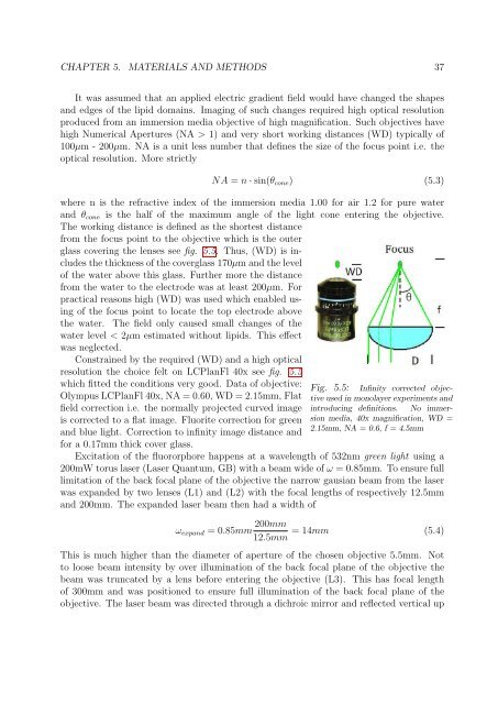
The working distance is defined as the shortest distance
from the focus point to the objective which is the outer
glass covering the lenses see fig. 5.5. Thus, (WD) is includes
the thickness of the coverglass 170µm and the level
of the water above this glass. Further more the distance
from the water to the electrode was at least 200µm. For
practical reasons high (WD) was used which enabled using
of the focus point to locate the top electrode above
the water. The field only caused small changes of the
water level < 2µm estimated without lipids. This effect
was neglected.
Constrained by the required (WD) and a high optical
resolution the choice felt on LCPlanFl 40x see fig. 5.5
which fitted the conditions very good. Data of objective: Fig. 5.5: Infinity corrected objective
used in monolayer experiments and
Olympus LCPlanFl 40x, NA = 0.60, WD = 2.15mm, Flat
field correction i.e. the normally projected curved image introducing definitions. No immersion
media, 40x magnification, WD =
is corrected to a flat image. Fluorite correction for green
2.15mm, NA = 0.6, f = 4.5mm
and blue light. Correction to infinity image distance and
for a 0.17mm thick cover glass.
Excitation of the fluororphore happens at a wavelength of 532nm green light using a
200mW torus laser (Laser Quantum, GB) with a beam wide of ω = 0.85mm. To ensure full
limitation of the back focal plane of the objective the narrow gausian beam from the laser
was expanded by two lenses (L1) and (L2) with the focal lengths of respectively 12.5mm
and 200mm. The expanded laser beam then had a width of
ω expand = 0.85mm 200mm
12.5mm
= 14mm (5.4)
This is much higher than the diameter of aperture of the chosen objective 5.5mm. Not
to loose beam intensity by over illumination of the back focal plane of the objective the
beam was truncated by a lens before entering the objective (L3). This has focal length
of 300mm and was positioned to ensure full illumination of the back focal plane of the
objective. The laser beam was directed through a dichroic mirror and reflected vertical up