CHAPTER 6: SPATIAL RESOLUTION 6.1 Definition and ...
CHAPTER 6: SPATIAL RESOLUTION 6.1 Definition and ...
CHAPTER 6: SPATIAL RESOLUTION 6.1 Definition and ...

You also want an ePaper? Increase the reach of your titles
YUMPU automatically turns print PDFs into web optimized ePapers that Google loves.
Physics of Medical X-Ray Imaging (1) Chapter 6<br />
<strong>CHAPTER</strong> 6: <strong>SPATIAL</strong> <strong>RESOLUTION</strong><br />
<strong>6.1</strong> <strong>Definition</strong> <strong>and</strong> Measurement of Spatial Resolution<br />
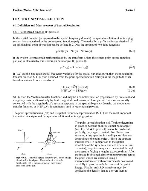
6.<strong>6.1</strong> Point spread function (Figure <strong>6.1</strong>)<br />
In the spatial domain, (as opposed to the spatial frequency domain) the spatial resolution of an imaging<br />
system is characterized by its point-spread function (psf). Theoretically, a psf is the image obtained of<br />
an infinitesimal point object that can be defined in 2-D as the product of two delta functions<br />
point(x,y) = δ(x,y) = δ(x) δ (y) (6-1)<br />
If the system is represented mathematically by the transform S then the system point spread function<br />
psf(x,y) is obtained by transforming a point object (Figure <strong>6.1</strong>).<br />
psf(x,y) = S [point(x,y)] (6-2)<br />
If (u,v) are the conjugate spatial frequency variables for the spatial variables (x,y), then the modulation<br />
transfer function MTF(u,v) is obtained from the point spread function psf(x,y) as the magnitude of its<br />
two-dimensional Fourier transform<br />
STF(u,v) = I{ psf(x,y)} (6-3)<br />
MTF(u,v) = |STF(u,v)|<br />
(6-3a)<br />
STF(u,v) is the “system transfer function” <strong>and</strong> may be a complex function (represented by finite real <strong>and</strong><br />
imaginary parts or alternatively by finite magnitude <strong>and</strong> non-zero phase parts). Since we are mostly<br />
concerned with the magnitude of a systems response in the spatial frequency domain, the modulation<br />
transfer function, or MTF(u,v), is commonly used in radiological physics.<br />
The point spread function (psf) <strong>and</strong> its spatial frequency representation (MTF) are the most important<br />
theoretical descriptors of the spatial resolution of an imaging system.<br />
x<br />
δ(x,y)<br />
object<br />
y<br />
x<br />
image<br />
psf(x,y)<br />
Figure <strong>6.1</strong>. The point spread function (psf) of the image<br />
of an ideal point object. The modulation transfer<br />
function (MTF) is the magnitude of the Fourier<br />
transform of the psf.<br />
y<br />
The point spread function is difficult to determine<br />
in practice because an infinitesimal point object<br />
(i.e., Eq. 6-1 & Figure <strong>6.1</strong>) cannot be produced<br />
perfectly, only approximated. For film-screen<br />
systems, a tiny aperture in a radiopaque plate can<br />
approximate the point object. Since the aperture<br />
must be small in comparison to the spatial<br />
resolution of the system (a few tens of microns in<br />
diameter), very few x-rays are transmitted through<br />
the aperture forcing a lengthy exposure time. After<br />
the image is obtained, density measurements across<br />
the point image are obtained using a<br />
microdensitometer with measurements positioned<br />
carefully to pass through the center of the point<br />
image. Finally, an H&D transform must be<br />
applied to the density data to convert them to
Physics of Medical X-Ray Imaging (2) Chapter 6<br />
relative exposure (required for linearity purposes).<br />
The conversion to relative exposure is required for all resolution measurements <strong>and</strong> will be assumed to<br />
be a part of the measurement process throughout the remainder of the chapter.<br />
<strong>6.1</strong>.2 Line spread function (Figure 6.2)<br />
Measuring the line-spread function can reduce the technical difficulties associated with obtaining <strong>and</strong><br />
measuring the point-spread function. As its name suggests, the line spread function is obtained with an<br />
infinitesimal slit in an opaque object, rather than an infinitesimal point aperture. The line-spread<br />
function is a one-dimensional representation of the two-dimensional point-spread function. Since we<br />
assume that the psf of the imaging system is space invariant, we can measure the shape of the linespread<br />
function (lsf) with a microdensitomer passing through the image of the slit, perpendicular to the<br />
slit length. As for the point spread function, the width of the slit must be sufficiently narrow so that its<br />
finite extent does not contribute significantly to the width of the image. That is, the spread in the<br />
imaged slit must be due almost entirely to the blurring contributed by the imaging system rather than the<br />
width of the slit. For film-screen systems, a slit width of 10 microns or smaller is required for this<br />
measurement.<br />
Mathematically, the slit (or line source) is defined as<br />
+∞<br />
∫<br />
line ( x)<br />
= δ ( x)<br />
= δ ( x)<br />
δ ( y)<br />
dy = point( x,<br />
y)<br />
dy<br />
−∞<br />
+∞<br />
∫<br />
−∞<br />
(6-4)<br />
which is narrow in the x-direction <strong>and</strong> extends indefinitely in the y-direction. If S is the linear transform<br />
of the imaging system, then we know that the line spread function lsf(x) is obtained by transforming the<br />
line source<br />
⎡⎡ +∞<br />
⎤⎤ +∞<br />
+∞<br />
lsf (x) = S[line(x)] = S⎢⎢<br />
∫ point(x, y)dy⎥⎥ = ∫ S[ point(x, y) ]dy = ∫ [ psf (x, y) ]dy<br />
(6-5)<br />
⎣⎣<br />
⎦⎦<br />
−∞<br />
−∞<br />
−∞<br />
€<br />
Input: f(x,y) = d(x)<br />
Output: g(x,y) = lsf(x)<br />
so that the line spread function lsf(x) is equal<br />
to the integral across y of the point spread<br />
function.<br />
Figure 6-02<br />
Figure 6.2. The line spread function (lsf) if the image of an<br />
ideal line object (e.g., infinitesimal slit in a lead plate). The<br />
MTF in one dimension is the magnitude of the Fourier<br />
transform of the lsf.<br />
y<br />
y<br />
Although the MTF of the system is defined<br />
from the Fourier transform of the pointspread<br />
function, it also is possible to obtain<br />
the MTF from the line-spread function by<br />
taking the Fourier transform of the line<br />
spread function. (If the slit is not a deltafunction<br />
with respect to the detector, then the<br />
MTF is obtained by dividing the Fourier<br />
transform of the line-spread function by the<br />
Fourier transform of the object (e.g. the slit).<br />
Care must be taken, of course, where the<br />
Fourier transform of the slit equals zero.)
Physics of Medical X-Ray Imaging (3) Chapter 6<br />
Mathematically,<br />
+∞<br />
+∞⎡⎡<br />
+∞ ⎤⎤<br />
I{lsf (x)} = ∫ lsf (x)e −2πiux dx = ∫ ⎢⎢ ∫ psf (x, y)dy⎥⎥ e −2πiux dx<br />
6-7)<br />
⎣⎣<br />
⎦⎦<br />
−∞<br />
−∞<br />
−∞<br />
€<br />
+∞ +∞<br />
= ∫ ∫ psf (x, y) e −2πi(ux +0y) dxdy = I{psf (x,y)} v= 0<br />
= STF(u,0) (6-8)<br />
−∞ −∞<br />
Hence the Fourier transform of the line-spread function is the STF evaluated in one dimension (recall<br />
that MTF = |STF|). If the lsf is circularly symmetric, then this expression completely specifies the MTF<br />
on the frequency € plane. We usually test the lsf parallel <strong>and</strong> perpendicular to the anode-cathode axis at<br />
the center of the field of view.<br />
<strong>6.1</strong>.3 Edge response function (Figure 6.3)<br />
A final method to define the spatial resolution of an imaging system is in terms of its "edge-response"<br />
function. In this technique, the source is presented with an object that transmits radiation on one side of<br />
an edge, but is perfectly attenuating on the other. Hence, its transmission is defined according to the<br />
equation<br />
⎧⎧<br />
(6-9)<br />
step(x, y) = ⎨⎨<br />
1 if x ≥ 0<br />
⎩⎩ 0 if x < 0<br />
As Barrett <strong>and</strong> Swindell point out, this function (Eq 6-9) also can be written as<br />
€ step(x, y) = step(x) = δ(x' )dx' =<br />
x<br />
∫<br />
−∞<br />
x<br />
∫<br />
−∞<br />
line(x' )dx'<br />
(6-10)<br />
If the system operator S is linear (Eq 5-42), <strong>and</strong> treating the integral as a generalized summation yields<br />
⎧⎧ x<br />
⎪⎪<br />
⎫⎫ x<br />
x<br />
⎪⎪<br />
esf (x) = S{step(x)} = S⎨⎨<br />
∫ line(x' )dx' ⎬⎬ =<br />
⎩⎩ ⎪⎪<br />
−∞ ⎭⎭ ⎪⎪ ∫ S{line(x' )}dx' = ∫ lsf (x' )dx'<br />
−∞<br />
−∞<br />
so that the line spread function is the derivative of the edge-spread function<br />
lsf (x) = d dx<br />
esf (x)<br />
Hence, we obtain a density profile<br />
Input: f(x) = step(x)<br />
Output: g(x) = esf(x)<br />
to determine the edge-spread<br />
function when imaging an edge. €<br />
The derivative of the edge-spread<br />
function is the line-spread<br />
function, the Fourier transform of<br />
which yields the MTF in one<br />
dimension according to equation<br />
6-3.<br />
(6-11)<br />
[ ] (6-12)<br />
y<br />
Figure 6.3. The edge spread function (esf) is the image of an ideal step object<br />
(e.g., edge of a lead plate). The lsf can be derived as the spatial derivative of<br />
the esf; similarly a line object is modeled as the derivative of an edge object.<br />
y
Physics of Medical X-Ray Imaging (4) Chapter 6<br />
6.2 Components of Unsharpness<br />
Now that we have described unsharpness mathematically, we can use these tools to study <strong>and</strong> quantify<br />
several components to unsharpness. We will consider four principal components. Geometric<br />
unsharpness refers to the loss of detail with increasing size of the radiation source. Motion unsharpness<br />
refers to the loss of detail due to motion of the source, the detector, or the object being imaged.<br />
Detector-unsharpness refers to the loss of detail caused by the resolving power of the detector.<br />
Digitization unsharpness refers to the loss of detail associated with the analog-to-digital conversion of<br />
the image.<br />
6.2.1 Geometric unsharpness<br />
Geometric unsharpness in a projection radiograph refers to the loss in image detail caused by the size of<br />
the focal spot of the x-ray tube. As shown in Figure 6.4, an extended x-ray source will blur the<br />
appearance of the edge or any other detailed object structure. We can use language borrowed from<br />
astronomy in describing the extent of this blurriness. The area directly behind the object, which is<br />
completely contained within the shadow of the object, is called the umbra. Similarly, the region that has<br />
a in a partial shadow of the focal spot <strong>and</strong> is called the penumbra. In some texts, the penumbra is called<br />
the edge gradient. (Note: umbra is Latin for shadow <strong>and</strong> paene is Latin for almost. “Umbrella” has<br />
similar Latin roots.)<br />
Obviously, as the size the focal spot increases, the size of the penumbra increases <strong>and</strong> the degree of<br />
geometrical unsharpness or blurriness also increases. Therefore, to obtain the most detail in the image,<br />
one should use the smallest focal spot possible. However, the focal spot must be large enough to<br />
dissipate the heat generated on the anode. This fundamental limitation forces many diagnostic medical<br />
procedures to utilize x-ray tubes with focal spots at least 1 mm wide.<br />
GEOMETRIC UNSHARPNESS<br />
Point Source<br />
Finite Source<br />
Object<br />
Object<br />
Umbra<br />
Detector<br />
Plane<br />
Penumbra or Edge-<br />
Gradient<br />
Umbra<br />
Detector<br />
Plane<br />
Image<br />
Density<br />
Image<br />
Density<br />
Figure 6.4. Geometric unsharpness is the loss of detail with increasing x-ray tube focal spot size. The umbra<br />
is the completely shadowed region behind the object while the penumbra is the partially shadowed region<br />
surrounding the umbra.
Physics of Medical X-Ray Imaging (5) Chapter 6<br />
Another important factor affecting geometric unsharpness is object magnification (M). As we<br />
previously found in Chapter 5, if the object is projected onto the image receptor with a magnification M,<br />
the focal spot is magnified by a factor of M-1. When the object is half way between the source <strong>and</strong><br />
detector, it is imaged with a magnification of 2, while the projected focal spot size is equal to its<br />
physical size (i.e. magnification equal to M-1= 1). As the object is moved closer to the detector object<br />
magnification tends toward unity while source or focal spot magnification tends toward zero. As the<br />
object is brought closer to the source, the magnification of both the object <strong>and</strong> the focal spot increases,<br />
causing increased geometric unsharpness (Figure 6.5). The increase in geometric unsharpness that<br />
accompanies magnification limits the degree to which magnification can be used to increase the spatial<br />
resolution with which the object is imaged.<br />
EFFECT OF MAGNIFICATION ON GEOMETRIC UNSHARPNESS<br />
Large Magnification<br />
Finite<br />
Source<br />
Small Magnification<br />
Finite<br />
Source<br />
Object<br />
Object<br />
Penumbra<br />
Umbra<br />
Penumbra<br />
Umbra<br />
Detector<br />
Plane<br />
Detector<br />
Plane<br />
Figure 6.5. Both source (focal spot) <strong>and</strong> object magnification decrease as object is moved closer to the detector<br />
plane. The impact of geometric unsharpness associates with the size of the penumbra relative to the umbra.<br />
Geometric unsharpness can be modeled mathematically using linear systems analysis presented<br />
previously in equation (5-67) of Chapter 5. In this formulation an image g(x,y) is obtained by<br />
convolving the object f(x,y) with the point-spread function h(x,y) due focal spot blurring only. This is<br />
expressed mathematically as<br />
g(x, y) =<br />
1<br />
M −1<br />
x<br />
f , y ( ) 2 M M<br />
( ) ⊗ ⊗h( −x , −y<br />
M −1 M −1) (6-13)<br />
or in the frequency domain,<br />
€<br />
G(u,v) = M 2 F(Mu,Mv) H(-(M-1)u,-(M-1)v) (6-14)
Physics of Medical X-Ray Imaging (6) Chapter 6<br />
where H(u,v) is the two dimensional transfer function associated with blurring by the focal spot. Both<br />
f(x,y) <strong>and</strong> F(u,v) refer to the object distributions (in spatial <strong>and</strong> frequency domains) which are magnified<br />
by a factor M onto the plane of the detector. If M>1 the projected image is larger than the object <strong>and</strong><br />
this can provide increased resolution when the detector is the limiting factor. Likewise, h(x,y) <strong>and</strong><br />
H(u,v) refer to the source or focal spot distributions where the source is magnified by a factor of M-1<br />
onto the plane of the detector. The negative signs in the arguments of h <strong>and</strong> H indicate that the image of<br />
the source distribution is spatially reversed. When M>2 the focal spot image is magnified potentially<br />
reducing detail in the final image. The trade-off between object magnification <strong>and</strong> focal spot<br />
magnification at the detector plane will be investigated later in this chapter after we discuss the effects<br />
of detector unsharpness. Note: Magnification or enlargement in the spatial domain is minification or<br />
contraction in the spatial frequency domain.<br />
6.2.2 Patient Motion (Motion Unsharpness)<br />
Ideal imaging systems assume that the patient, radiation source, <strong>and</strong> detector system are all stationary<br />
with respect to one another during a radiographic exposure. However, this is not true except in extreme<br />
cases, i.e. post mortem. When one or more of these components move, the image is blurred (loss of<br />
spatial resolution) due to "motion unsharpness". Patient motion is usually the major cause of motion<br />
unsharpness since movement of both the detector <strong>and</strong> the source can be controlled. The motion of the<br />
patient can be complex <strong>and</strong> uncontrollable, for example due to cardiac motion or peristaltic motion of<br />
the abdominal contents. While it is difficult to model patient motion exactly, a simple model can be<br />
employed to quantify this effect.<br />
Consider an object as of a pinhole aperture moving uniformly in the x-direction with a constant velocity<br />
v during the exposure time T. The displacement of the projected image in the plane of the detector, due<br />
to motion of the object, is MvT, where M is object magnification. Under these assumptions, a point<br />
object will take the form (Figure 6.6)<br />
h motion<br />
(x) = 1<br />
MvT II<br />
( ) (6-15)<br />
x<br />
MvT<br />
Point SourcePlane<br />
Object<br />
MOTION UNSHARPNESS<br />
h (x) =<br />
motion<br />
vT<br />
MvT<br />
1<br />
€<br />
Object moving with velocity<br />
v during time interval T<br />
MvT Π( MvT<br />
)<br />
Figure 6.6. Motion unsharpness is the loss of detail due<br />
to motion of the source, detector or the object. For<br />
uniform velocity, the motion can be characterized by a<br />
spread function as shown in this figure.<br />
x<br />
where the normalizing term 1/(MvT) in front of the<br />
rectangle function insures that the motion<br />
component of the point-spread function [h motion (x)]<br />
has unit area such that it approaches a delta function<br />
in the limit where either v or T approach zero (little<br />
motion or extremely short exposure time). This<br />
emphasizes that an obvious <strong>and</strong> effective method of<br />
limiting the effect of motion unsharpness is to use<br />
very short exposure times. For example, chest<br />
radiographs are taken with exposure times of 50 ms<br />
or less, to minimize the effect of cardiac motion <strong>and</strong><br />
to produce a sharp image of the cardiac border.<br />
6.2.3 Film-Screen Unsharpness<br />
Unsharpness is also caused by light diffusion in the
Physics of Medical X-Ray Imaging (7) Chapter 6<br />
intensifying screen. When x-rays are absorbed at depth in the intensifying screen, the light diffuses,<br />
contributing to unsharpness. A thicker screen will allow more light diffusion <strong>and</strong> therefore will<br />
contribute more to unsharpness. The resolution varies from 6-9 lp/mm for images made with fast (i.e.<br />
thick) screens to 10-15 lp/mm for images obtained with detail screens under laboratory conditions. The<br />
resolution is much poorer (2-4 lp/mm) for fluoroscopic images obtained using an image intensifier. The<br />
light diffusion, <strong>and</strong> therefore the degree of screen unsharpness, can be limited in detail screens by tinting<br />
the phosphor layer of the intensifying screen. Do you know why<br />
Unsharpness contributed by film is, in most clinical examinations, negligible in comparison to either<br />
geometric or screen unsharpness. The MTF of film is ~ 50% at a spatial frequency of 20 lp/mm, while<br />
that of a screen drops to ~50% at about 2 lp/mm, so the drop in resolution is principally due to the screen<br />
as frequencies about 1-2 lp/mm. The bottom line is that modern radiological practice uses screens for all<br />
medical diagnosis so film unsharpness is not a limitation in overall system sharpness.<br />
Following the arguments presented by Macovski <strong>and</strong> referring to Figure 6.7 we will calculate the<br />
exposure to the film emulsion by light photons emitted by the intensifying screen. Assume that a x-ray<br />
photon is absorbed at a distance x within an intensifying screen. We will establish a coordinate system<br />
with an origin placed at the site of interaction. Let r be the perpendicular distance along the plane of the<br />
film emulsion from the point of light measurement to the x-ray interaction site, <strong>and</strong> let d be the thickness<br />
of the intensifying screen.<br />
Film exposure is proportional to the integrated fluence (i.e. number of photons per unit area) of light<br />
photons reaching the emulsion. At r = 0, that is at the position directly in line with the interaction site,<br />
the fluence depends only on the depth of interaction x. Because the light photons are assumed to be<br />
isotropically radiated, the screen response at r = 0 follows an inverse square law<br />
h(0, x) = k x 2 (6-16)<br />
where k is a constant of proportionality that relates the generation <strong>and</strong> propagation of light in the<br />
intensifying screen following the absorption of the x-ray photon. At a distance “r” from the origin, the<br />
light fluence falls off due to an inverse € square law, <strong>and</strong> also is modulated by a cosine term due to the<br />
obliquity with which the light photons strike the film emulsion. Therefore,<br />
⎛⎛ 1 ⎞⎞<br />
h(r,x) = k⎜⎜<br />
⎟⎟ cos(θ) = k<br />
⎝⎝ r 2 + x 2 ⎠⎠<br />
x<br />
( r 2 + x 2<br />
) (6-17)<br />
3 / 2<br />
We assume that this system is spaceinvariant<br />
so that the frequency<br />
response of the system € is given by<br />
the Fourier transform of the pointspread<br />
function h(r). We can<br />
determine its spatial frequency<br />
behavior in polar coordinates for a<br />
function having circular symmetry<br />
using the Hankel transform H<br />
(Appendix 6-1).<br />
r<br />
θ<br />
p<br />
h<br />
o<br />
t<br />
x-ray<br />
x<br />
Film<br />
Intensifying<br />
screen<br />
Figure 6.7. An x-ray photon is absorbed at a depth x in an intensifying<br />
screen. Light is emitted by the phosphor at an angle q <strong>and</strong> interacts<br />
with the film at a distance r from the path of the x-ray photon
Physics of Medical X-Ray Imaging (8) Chapter 6<br />
Bracewell (p.249) shows that<br />
which can be applied to equation 6-17 yielding,<br />
H 0<br />
(ρ,x) € = H{h(r,x)} = 2π<br />
3<br />
⎡⎡<br />
H 1 ⎤⎤ 2<br />
⎣⎣ ⎢⎢ a 2 + r 2 ⎦⎦ ⎥⎥ = 2πe −2πaρ<br />
a<br />
∞<br />
∫<br />
0<br />
⎛⎛ ⎜⎜<br />
⎝⎝<br />
kx<br />
r 2 +x 2<br />
⎞⎞<br />
⎠⎠<br />
⎟⎟ 3<br />
J 0<br />
(2πρr)rdr = 2πe−2πxρ<br />
x<br />
(6-18)<br />
(6-19)<br />
where J 0 is the Bessel function of the zeroth order.<br />
€<br />
For convenience, we will normalize the frequency response to give unit response at a spatial frequency<br />
of ρ = 0,<br />
H ( ρ,<br />
x)<br />
=<br />
(6-20)<br />
The function H*(ρ,x) gives the average frequency response per photon interacting at a depth x in the<br />
intensifying screen. When a beam of photons interacts with the intensifying screen, we must calculate<br />
the response due to all photons interacting with the screen, regardless of depth. If we assume that p d (x)<br />
is the fraction of all incident photons interacting per unit thickness at a depth x in the intensifying screen<br />
(i.e. the probability density function), then the average transfer function for this beam of interacting x-<br />
rays is<br />
H ( ρ)<br />
=<br />
∞<br />
∫<br />
0<br />
(6-21)<br />
To determine p d (x), we observe that the fractional number of photons transmitted through a distance x of<br />
an infinitely thick intensifying screen is e - µ x<br />
so that the fraction of photons removed up to a distance x is<br />
P(x) = 1 – e - µ x<br />
(6-22)<br />
The probability density function is the rate at which the photons are removed per unit length in the<br />
intensifying screen<br />
p d<br />
(x) = d P<br />
dx [ d<br />
(x)] = µe −µx (6-23)<br />
However, equation 6-23 applies only to the unrealistic case of an infinitely thick intensifying screen.<br />
For an intensifying screen of finite thickness d, the fraction of photons removed up to a distance x is<br />
€<br />
P’(x) =<br />
H<br />
0(<br />
ρ,<br />
x)<br />
= e<br />
H (0, x)<br />
* −<br />
0<br />
2πxρ<br />
*<br />
−2πρx<br />
H ( ρ,<br />
x)<br />
pd ( x)<br />
dx = e pd<br />
( x)<br />
dx<br />
∞<br />
∫<br />
0<br />
−µ<br />
x<br />
probability of photon interaction up to distance x<br />
probability of photon interaction in screen of thickness d = 1−<br />
e<br />
−µ<br />
d<br />
1−<br />
e<br />
where the expression above has been normalized with using the number of photons absorbed in the<br />
screen so that P ’ d(x) represents the fraction of absorbed photons up to the distance x. The probability<br />
(6-24)
Physics of Medical X-Ray Imaging (9) Chapter 6<br />
density function p d (x) for an intensifying screen of finite thickness d therefore is<br />
p d<br />
(x) = d P ' dx [ d (x)] = µe−µx<br />
(6-25)<br />
−µd<br />
1− e<br />
Therefore, from equation 6-21<br />
∞<br />
∫<br />
H(ρ) = € H * (ρ,x) p d<br />
(x)dx =<br />
0<br />
µ<br />
1−e − µd<br />
d<br />
∫<br />
0<br />
e −2πρx e −µx dx<br />
(6-26)<br />
€<br />
Note that as ρ approaches 0 then H(ρ) approaches unity as expected. For high spatial frequencies<br />
(where ρ is large), we know that<br />
€<br />
=<br />
(6-26a)<br />
e − d ( 2πρ +µ ) ≈ 0<br />
<strong>and</strong> 2πρ >> µ, so we have<br />
µ<br />
H(ρ) ≈<br />
(2πρ)(1− e −µd )<br />
(6-28)<br />
€<br />
The transfer function H(ρ) of the intensifying screen in (6-28) therefore gives the system frequency<br />
response as we approach a high frequency limit. For best spatial resolution we obviously want the value<br />
of H(ρ) to be as large € (i.e. close to 1) as possible at higher frequencies. In this regard, equation 6-28<br />
shows there is a trade-off between screen thickness <strong>and</strong> spatial resolution. As the screen thickness d is<br />
increased, the efficiency of the screen increases reducing radiation dose to the patient. However,<br />
increasing the screen thickness d decreases H(ρ), reducing high frequency response. Alternatively,<br />
decreasing the screen thickness d increases the system response H(ρ), increasing spatial resolution while<br />
requiring increased patient radiation dose. With this trade-off in mind, it is important to choose<br />
phosphor materials with the highest possible efficiency (i.e. large values of µ), so that the patient<br />
radiation dose can be minimized while increasing H(ρ) to maximize signal amplitudes. Practically, even<br />
though the most efficient phosphors are used in modern intensifying screens, manufacturers offer<br />
intensifying screens having a range of phosphor thickness so that the practitioner can select the screen<br />
that offers sufficient spatial resolution with the highest possible photon absorption efficiency.<br />
6.2.4 Digital image resolution<br />
µ<br />
[1− (2πρ +µ )(1−e − µd ) e−d(2πρ +µ) ]<br />
We have represented an image g(x,y) as the convolution between the object transmission f(x,y) <strong>and</strong> the<br />
point-spread function h(x,y) of the imaging system,<br />
g(x, y) = f<br />
x<br />
( , y M M ) ⊗ ⊗h −x , −y<br />
M −1 M −1<br />
( ) (6-29)<br />
where both the object <strong>and</strong> the point spread function are corrected for magnification M when projected<br />
onto the plane of the image detector (Note: the point spread function is assumed to be normalized so that<br />
we don’t have to keep track € of other scale factors). The object term may contain blurring due to patient<br />
motion or other contributors to motion unsharpness, although these factors will be ignored in this<br />
discussion. Our goal here is to represent the digital image mathematically in terms of the analog image
Physics of Medical X-Ray Imaging (10) Chapter 6<br />
g(x,y), <strong>and</strong> to evaluate the frequency characteristics of the digitized signal.<br />
A two-step process can represent digitization, we first sample the analog image, then "pixellate" the<br />
sampled image data. When we sample the image, we select regularly spaced values from the analog<br />
values that we assign to the rectangular pixels during the pixellation process. Mathematically, in one<br />
dimension, let g(x) represent the analog image from which we wish to generate the digital image with a<br />
pixel spacing of a. Sampling is done by multiplication of the image g(x) by the comb function III(x/a)<br />
<strong>and</strong> pixellation is done by convolving the sampled data with a box function II(x/a)<br />
g dig (x) = [g(x) III(x/a)] ⊗ II(x/a) (6-30)<br />
where the width (a) of the box function (pixel dimension) is selected to match the sample spacing<br />
(Figure 6-8).<br />
Intuitively, we suffer a loss of spatial resolution if pixel dimensions are large compared to details we<br />
wish to preserve in the image. The sampling process also can introduce aliasing (i.e. a false frequency<br />
signal) if the sampling frequency does not satisfy Shannon's theorem (i.e. the sampling frequency must<br />
be twice the highest spatial frequency in the image).<br />
Several effects of the digitization process are best seen using the frequency domain representation of<br />
equation 6-30<br />
G dig (u)= a 2 [G(u) ⊗ III(au)] sinc(au) (6-31)<br />
In this equation, we see that in the frequency domain the digitization process is begun by convolving the<br />
Fourier transform G(u) of the image function with the comb function III(au). Since the comb function is<br />
the sum of an infinite number of regularly spaced delta functions, this convolution replicates G(u) at<br />
equally spaced intervals Δu = 1/a on the spatial frequency axis. The replicates of G(u) are further<br />
modified by multiplication by the sinc function. This serves to suppress the amplitude of the sampled<br />
function [g(x) III(x/a)] at higher spatial frequencies since the magnitude of the sinc function decreases<br />
with increasing spatial frequency. This reflects the loss of detail associated with convolution width of<br />
the box function in (6-30).<br />
The replication term [G(u) ⊗ III(au)] suggests the possibility of aliasing in the sampled function [g(x)<br />
III(x/a)]. In particular, if adjacent replicates of G(u) overlap in the frequency domain, then aliasing<br />
occurs (Figure 6-9). As can be seen in Figure 6-10, if the highest spatial frequency in the analog image<br />
is u obj [lp/distance] <strong>and</strong> the sampling frequency is u samp [samples/distance], then if u samp < 2u obj , then G(u)<br />
is aliased. This shows up as the overlapping of the replicates in the frequency interval from u samp - u obj<br />
up to the maximum frequency of u obj /2. This figure illustrates the origin of the similar statement in<br />
Chapter 3 that the frequency of the aliased signal equals the sampling frequency (u samp ) minus the presampled<br />
frequency (u obj ).
Physics of Medical X-Ray Imaging (11) Chapter 6<br />
Image Digitization<br />
Spatial Domain<br />
Spatial Frequency Domain<br />
Image Density<br />
Analog Image g(x)<br />
Spatial Frequency<br />
Amplitude<br />
Fourier Transform G(u)<br />
Position<br />
Spatial Frequency<br />
Image Density<br />
x<br />
Sampling g(x) III (<br />
a<br />
)<br />
Spatial Frequency<br />
Amplitude<br />
Replication [a G(u) ⊗ III (au)]<br />
Image Density<br />
Position<br />
Pixellation [g(x) III( x<br />
a<br />
)] ⊗II( x<br />
a<br />
)<br />
Spatial Frequency<br />
Amplitude<br />
Spatial Frequency<br />
Modulation<br />
[a G(u) ⊗ III (au)] [a sinc(au)]<br />
Image Density<br />
Position<br />
Digital Image g<br />
dig<br />
(x)<br />
Spatial Frequency<br />
Amplitude<br />
Spatial Frequency<br />
Spatial Frequency Representation<br />
[a G(u) ⊗ III (au)] [a sinc(au)]<br />
Position<br />
Figure 6-8: Image Digitization<br />
Spatial Frequency<br />
Figure 6-8. The process of image digitization begins with sampling of an analog image followed by pixellation. This<br />
process is illustrated in both spatial <strong>and</strong> spatial frequency domains.
Physics of Medical X-Ray Imaging (12) Chapter 6<br />
Aliasing Due to Incomplete Digital Sampling<br />
Spatial Domain<br />
Spatial Frequency Domain<br />
Analog Image g(x)<br />
Fourier Transform G(u)<br />
Position<br />
Spatial Frequency<br />
Sampling g(x) III (x/a)<br />
Replication [a G(u) ⊗ III (au)]<br />
Position<br />
Aliasing<br />
Spatial Frequency<br />
Figure 6-9. Aliasing is due to undersampling of an analog signal during digitization. This<br />
introduces false information in the spatial frequency domain.<br />
We can prevent aliasing by smoothing (or "b<strong>and</strong>-limiting") an analog signal g(x) before sampling if the<br />
maximum frequency in the smoothed image is less than 1/2 the sampling frequency (Figure 6-10).<br />
Mathematically, if smoothing is performed by convolving the analog image g(x) with a low-pass kernel<br />
b lp (x), the digitized image can be expressed as<br />
g dig (x) = {[g(x) ⊗ b lp (x)] III(x/a)} ⊗ II(x/a) (6-32)<br />
which in the spatial frequency domain is equivalent to<br />
G dig (u) =a 2 {[G(u) B lp (u)] ⊗ III(au)}sinc(au) (6-33)<br />
where B lp (u)is the Fourier transform of the smoothing or blurring function b lp (x). The blurring process<br />
has two important advantages. First, it can improve the signal-to-noise ratio of the digitized image by<br />
removing high spatial frequency components that often are dominated by noise. Second, blurring can<br />
reduce or eliminate aliasing (Figure 6-10). Of course, the function b lp (x) must be chosen carefully to<br />
reduce aliasing <strong>and</strong> improve the signal-to-noise ratio of the digitized image, without unacceptable loss of<br />
spatial resolution.
Physics of Medical X-Ray Imaging (13) Chapter 6<br />
Aliasing <strong>and</strong> B<strong>and</strong> Limiting (Smoothing) the Image<br />
In the Spatial Frequency Domain<br />
Spatial Frequency<br />
Amplitude<br />
Fourier Transform G(u)<br />
Sampling<br />
Spatial Frequency<br />
Amplitude<br />
Replication [a G(u) ⊗ III (au)]<br />
Aliasing (region of overlap)<br />
u obj<br />
Spatial<br />
Frequency<br />
u samp<br />
- u obj<br />
u samp<br />
Spatial<br />
Frequency<br />
Spatial Frequency<br />
Amplitude<br />
Smoothing<br />
(B<strong>and</strong>-Limiting)<br />
G(u) with low-pass<br />
filter H lp (u)<br />
Fourier Transform<br />
G(u) H lp (u)<br />
Sampling<br />
Spatial Frequency<br />
Amplitude<br />
Replication [a G(u) H<br />
No Aliasing (no overlap)<br />
(u)<br />
lp<br />
]⊗ III (au)<br />
u obj<br />
Spatial<br />
Frequency<br />
u samp<br />
Spatial<br />
Frequency<br />
Figure 6-10. Alaising can be removed by smoothing or b<strong>and</strong>-limiting the analog signal prior to sampling. This removes<br />
regions of replicate overlap in the spatial frequency domain of the sampled signal.<br />
6.3 Trade-Offs Between Geometric Unsharpness <strong>and</strong> Detector Resolution<br />
There is a fundamental trade-off between the increase in object detail that can be seen due to image<br />
magnification <strong>and</strong> the decrease in object detail due to increased geometric unsharpness (source<br />
magnification). Object detail increases with increasing magnification if system resolution is limited due<br />
to poor spatial resolution of the detector. On the other h<strong>and</strong>, geometric unsharpness decreases object<br />
detail due to the magnified focal spot or point spread function, so we seek a trade-off value for M that<br />
can best preserve the desired detail.<br />
If an image is recorded with object magnification M, <strong>and</strong> if the focal spot is expressed as a rectangle of<br />
width a, the width of the focal spot when projected onto the detector plane is (M-1)a. This width is<br />
( M −1)a<br />
equals when back projected to the object plane. We can characterize geometric unsharpness in<br />
M<br />
the object plane as the cut-off frequency “u s “ associated with the geometric point spread function [H(u)].<br />
The cut-off frequency is defined as the frequency where H(u) first goes to zero. Since h(x) is a rectangle<br />
function H(u) will be a sinc function, <strong>and</strong> we know that 1/width of a rectangle function h(x) is the cutoff<br />
frequency of the sinc function. Therefore, u s = 1/width <strong>and</strong> expressed in terms of M <strong>and</strong> a is<br />
u M<br />
= s ( M −1 )<br />
(6-34)<br />
a
Physics of Medical X-Ray Imaging (14) Chapter 6<br />
Similarly, detector resolution modeled as a rectangle of width b in the plane of the detector corresponds<br />
to a width of M<br />
b in the object plane, giving a detector cut-off frequency of<br />
M<br />
u d<br />
= (6-35)<br />
b<br />
We can investigate the trade-off between u d <strong>and</strong> u s with increasing object magnification by graphing<br />
them as a function of object magnification.<br />
Object<br />
Plane<br />
GEOMETRIC UNSHARPNESS<br />
Point<br />
Source<br />
Detector<br />
Resolution = b<br />
CUTOFF FREQUENCIES IN OBJECT PLANE<br />
u detector<br />
=<br />
M<br />
u<br />
b<br />
source<br />
=<br />
Source<br />
Width<br />
= a<br />
Projected source width<br />
= a(M-1)<br />
M<br />
(M-1)a<br />
This relationship is shown in Figure 6-11.<br />
The curve labeled "source" shows how<br />
increasing magnification leads to<br />
resolution loss (i.e. decreasing the cut-off<br />
spatial frequency) (Eq. 6-34). As we can<br />
see, in the limit of infinite magnification,<br />
the unsharpness due to the source<br />
asymptotically approaches the value<br />
u s<br />
= 1 a<br />
( lim M → +∞)<br />
(6-36)<br />
SYSTEM <strong>RESOLUTION</strong> vs. OBJECT MAGNIFICATION<br />
1<br />
b<br />
Source<br />
Optimal<br />
Magnification<br />
Slope 1<br />
b<br />
M=1 2 3 4 5<br />
Object Magnification<br />
Figure 6-11. Cut-off frequency analysis.<br />
Detector<br />
€<br />
Asymptotically<br />
Approaches 1<br />
a<br />
The curve labeled "detector" <strong>and</strong> Eq. 6-35<br />
show how magnification leads to resolution<br />
gain (i.e. increasing cut-off spatial<br />
frequencies) with increasing magnification.<br />
At unit magnification, the cut-off<br />
frequency for the detector is u d = 1/b, <strong>and</strong><br />
for larger object magnifications, the cut-off<br />
frequency increases with a slope of 1/b. At<br />
any M the lower of detector or source<br />
cut-off frequency determines the system<br />
cut-off frequency. Since the source cut-off<br />
frequency is monotonically decreasing with<br />
magnification <strong>and</strong> the object cut-off<br />
frequency is monotonically increasing, the maximum or optimal cut-off frequency occurs where their<br />
response curves cross (are equal). This occurs when b=(M-1)a. In theory, this is the magnification at<br />
which the imaging system should be operated since it yields the highest cut-off frequency. This tradeoff<br />
between greater focal spot blurring <strong>and</strong> better detector resolution at higher magnification is illustrated in<br />
the following example.
Physics of Medical X-Ray Imaging (15) Chapter 6<br />
The optimal combination of digitization, detector <strong>and</strong> geometrical components of resolution (or<br />
unsharpness) are explored in example 6-1.<br />
Example 6-1:<br />
Assume we are imaging a patient with an image intensifier system. The image intensifier has a<br />
resolution width of 0.2 mm <strong>and</strong> uses an x-ray tube with a focal spot width of 1 mm (both modeled as<br />
rectangle functions). The diameter of the image intensifier input phosphor is 15 cm <strong>and</strong> the video output<br />
is delivered to an image processor which can produce digital images in either a 512 X 512 format or a<br />
1024 X 1024 format. (For purposes of this problem, we will ignore the spatial resolution characteristics<br />
of the television camera, although generally this is a very important consideration.)<br />
(a) As a function of object magnification, graph the cut-off frequency for geometric unsharpness,<br />
detector unsharpness by the image intensifier, <strong>and</strong> unsharpness due to both the 512 X 512 image matrix<br />
as well as the 1024 X 1024 image matrix.<br />
(b) From the graph generated in (a) determine the highest possible cut-off spatial frequency first for a<br />
512 X 512 image, then for a 1024 X 1024 image. In each case, specify the object magnification at<br />
which this optimal system response occurs.<br />
Solution:<br />
(a) Let M be the object magnification. The x-ray tube has a focal spot width of 1 mm. Therefore, its<br />
object cut-off spatial frequency is given by<br />
M<br />
( M −1)(1<br />
mm)<br />
M<br />
( M −1)<br />
−1<br />
u s<br />
= = mm<br />
(6-37)<br />
The image intensifier has a resolution width of 0.2 mm <strong>and</strong> therefore has an object cut-off spatial<br />
frequency of<br />
u d = M/0.2 mm = 5.0 M mm-1 (6-38)<br />
The 512 X 512 matrix has a pixel width of<br />
a 512 = 150 mm/512 = 0.293 mm (6-39)<br />
This is modeled as a rectangle of width 0.293 mm/M in the object plane with a cut-off spatial frequency<br />
of M/0.293 mm = M 3.41 mm -1 . However, a more serious cut-off occurs at half this frequency due to<br />
sampling, i.e. the Nyquist frequency limit so the actual cut-off frequency is<br />
u 512<br />
=<br />
256 cycles<br />
150 mm / M = M 1.71 mm−1 (6-40)<br />
Finally, the 1024 X 1024 matrix has a pixel width of<br />
€<br />
a 1024 = 150 mm/1024 = 0.146 mm (6-41)
Physics of Medical X-Ray Imaging (16) Chapter 6<br />
with a corresponding Nyquist cut-off spatial frequency of<br />
u 1024<br />
=<br />
512 cycles<br />
= M 3.41 150 mm / M mm−1 (6-42)<br />
The graph of cut-off frequencies for the focal spot, image intensifier, 512x512 image matrix, <strong>and</strong> 1024x<br />
1024 image matrix is shown in Figure 6-12.<br />
€<br />
(b) When a 512 X 512 matrix is used, the detector resolution is limited by the matrix <strong>and</strong> focal spot size<br />
(geometric unsharpness) rather than the image intensifier. The optimal system response is achieved<br />
when the cut-off spatial frequency from the 512x512 image matrix equals that from the x-ray tube focal<br />
spot. This condition is determined by setting u 512 = u d <strong>and</strong> solving for M<br />
M = 1.586 (6-43)<br />
giving an optimal cut-off spatial frequency of<br />
u s<br />
M<br />
= mm<br />
( M −1)<br />
−1<br />
= 1.586/0.586 = 2.71 cycles<br />
mm<br />
(6-44)<br />
Even when a 1024 X 1024 matrix is used, the detector resolution is still limited by the image matrix <strong>and</strong><br />
geometric unsharpness. The optimal system response is similarly achieved when the cut-off frequency<br />
from the 1024 x 1024 image matrix equals that due to the x-ray tube focal spot (geometrical<br />
component). This condition is met when<br />
M = 1.292 (6-45)<br />
giving an optimal cut-off spatial frequency of<br />
u s<br />
M<br />
= mm<br />
( M −1)<br />
−1<br />
= 1.292/0.292 = 4.42 cycles<br />
mm<br />
(6-46)<br />
However, the system cutoff frequency increases dramatically <strong>and</strong> is achieved with less magnification.<br />
CUT-OFF <strong>SPATIAL</strong> FREQUENCY FOR AN IMAGE INTENSIFIER WITH<br />
A 1024 x 1024 or 512 x 512 DIGITAL IMAGE MATRIX<br />
12.00<br />
10.00<br />
8.00<br />
6.00<br />
M=1.20,<br />
u = 6.0<br />
M=1.29<br />
u = 4.42<br />
M = 1.59<br />
u = 2.71<br />
Image<br />
Intensifier<br />
1024x1024<br />
Matrix<br />
512x512<br />
Matrix<br />
4.00<br />
1 mm X-Ray Tube<br />
Focal Spot<br />
2.00<br />
0.00<br />
1 1.25 1.5 1.75 2 2.25<br />
Object Magnification<br />
Figure 6-12. In Example <strong>6.1</strong> at low object magnifications (M) the spatial resolution of<br />
the system is limited by digitization. The 1024x1024 matrix is better than the 512x512<br />
matrix. At higher object magnification (M) the spatial resolution is limited by blurring<br />
from the 1 mm focal spot of the x-ray tube.
Physics of Medical X-Ray Imaging (17) Chapter 6<br />
Appendix 6-1: The Hankel Transform <strong>and</strong> the Bessel Function<br />
It often is convenient to express equations <strong>and</strong> formulae in terms of polar coordinates (r,θ) rather than<br />
Cartesian coordinates (x,y). If we know the Cartesian coordinates of a point (x,y), we can obtain its<br />
polar coordinates through well-known transformations<br />
<strong>and</strong><br />
r 2 = x 2 + y 2<br />
(6-A1)<br />
θ = arctan( y x). (6-A2)<br />
Certain two-dimensional functions have circular symmetry. That is, if f(x,y) is a function of the<br />
two independent Cartesian coordinates (x,y), when expressed in terms of polar coordinates, the function<br />
f can € be specified entirely as a function of the radial coordinate r so that<br />
f(r) = f(x,y).<br />
(6-A3)<br />
An example of such a function would be<br />
f(x,y) = exp[-π(x 2 + y 2 )]<br />
(6-A4)<br />
which in polar coordinates is given by<br />
f(r,θ) = exp[-πr 2 ]<br />
(6-A5)<br />
Obviously, f(r,θ) is circularly symmetric because it is independent of the angular variable θ.<br />
If we can express a two-dimensional function f in terms of the single polar coordinate r (i.e. if f is<br />
circularly symmetric), then we can transform the Fourier transform from Cartesian to polar coordinates.<br />
In this case, the Fourier transform becomes the Hankel transform. If ρ is the spatial frequency variable<br />
corresponding to the spatial variable r, then the Hankel transform is defined by<br />
∞<br />
∫<br />
F( ρ)<br />
= 2π<br />
f ( r)<br />
J (2πρr<br />
rdr<br />
0<br />
0<br />
)<br />
(6-A6)<br />
while the inverse Hankel transform is defined by<br />
∞<br />
∫<br />
0<br />
f ( r)<br />
= 2π<br />
F(<br />
ρ)<br />
J (2πρr<br />
ρdρ<br />
0<br />
)<br />
(6-A7)<br />
where ρ is the conjugate spatial frequency variable for the spatial variable r (Eq 6-A1)<strong>and</strong><br />
ρ 2 = u 2 + v 2<br />
(6-A8)<br />
To derive equation 6-A6, we change to polar coordinates in the definition of the Fourier transform <strong>and</strong><br />
integrate over the angular variable. That is, if<br />
x = r cos θ <strong>and</strong> y = r sin θ<br />
(6-A9)
Physics of Medical X-Ray Imaging (18) Chapter 6<br />
are expressed in terms of the polar coordinates (r,θ), while the conjugate spatial-frequency variables<br />
u = ρ cos φ <strong>and</strong> v = ρ sin φ (6-A10)<br />
are expressed in terms of the polar coordinates (ρ,φ), then<br />
F(<br />
u,<br />
v)<br />
+∞ +∞<br />
−2πi ( ux+<br />
vy)<br />
= f ( x,<br />
y)<br />
e dxdy<br />
∫ ∫<br />
−∞ −∞<br />
(6-A11)<br />
F(<br />
u,<br />
v)<br />
+∞ +∞<br />
−2πir ρ (cosθ<br />
cosϑ+<br />
sinθ<br />
)<br />
= f ( x,<br />
y)<br />
e<br />
sin ϑ<br />
dxdy<br />
∫ ∫<br />
−∞ −∞<br />
(6-A12)<br />
F<br />
+∞2π<br />
−2πirρ<br />
cos( θ −ϑ<br />
)<br />
( u,<br />
v)<br />
= f ( r)<br />
e dθrdr<br />
∫ ∫<br />
−∞ 0<br />
(6-A13)<br />
F<br />
+∞2π<br />
−2πirρ<br />
cosθ<br />
( u,<br />
v)<br />
= f ( r)<br />
e dθrdr<br />
∫ ∫<br />
−∞ 0<br />
(6-A14)<br />
And using the relationship defining the zero order Bessel function of the first kind J o (z) where<br />
0<br />
)<br />
2π<br />
∫ − iz cosθ<br />
e<br />
0<br />
J ( z = dθ<br />
(6-A15)<br />
from equation 6-A14, the definition of the Fourier transform in polar coordinates for circularly<br />
symmetric functions becomes the Hankel transform H(ρ) where<br />
+∞<br />
∫<br />
0<br />
H ( ρ)<br />
= 2π<br />
f ( r)<br />
J (2πρr<br />
rdr<br />
0<br />
)<br />
(6-A16)
Physics of Medical X-Ray Imaging (19) Chapter 6<br />
<strong>CHAPTER</strong> 6: HOMEWORK PROBLEMS<br />
1. The value of the MTF of a system at 2 lp/mm is 0.25. Assuming three serial components contribute<br />
to system blurring <strong>and</strong> that two are identical with an MTF value of 0.7 at 2 lp/mm, calculate the MTF<br />
value of the third component at that frequency.<br />
2. During an experiment to measure the spatial frequency response of an imaging system, we obtain an<br />
edge spread function, described by normalized density measurements across which s presented in the<br />
graph below. Assume that the image unsharpness is due to penumbral effects from the source <strong>and</strong> that<br />
detector unsharpness is negligible. Also assume that the image is recorded with an object<br />
magnification of M = 2.<br />
1<br />
-a<br />
2<br />
a<br />
2<br />
(a) From the edge spread function shown above, show that the line spread function s(x) for the system is<br />
(b) Assume that we have a source distribution of<br />
lsf (x) = 1 II x a ( a).<br />
€<br />
t s<br />
(x) = 1 II x a ( a)<br />
<strong>and</strong> a new detector which has a detector point-spread function described by a rectangular function<br />
€<br />
t d<br />
(x) = 1 II x b ( b)<br />
When the effects of both geometric unsharpness <strong>and</strong> detector unsharpness are included, show that the<br />
MTF of the system is<br />
€<br />
MTF system (u) = | sinc(au) sinc(bu) |<br />
Moreover, if a = b, show that the point spread function of the system is given by the equation<br />
1<br />
psf ( x)<br />
=<br />
a<br />
Λ(<br />
x<br />
a<br />
)
Physics of Medical X-Ray Imaging (20) Chapter 6<br />
(c) If a ≠ b, sketch the point-spread function of the system <strong>and</strong> briefly justify your answer either<br />
conceptually or mathematically.<br />
3. A resolution pattern consists of equal width thin lead bars separated by equal widths of a radiolucent<br />
material (air, plastic, or thin aluminum). Assume that the spacing between adjacent lead bars equals the<br />
distance a, <strong>and</strong> that the width of the interspace material <strong>and</strong> of the lead bars are equal.<br />
Assume that we fix the distance between the x-ray source <strong>and</strong> the sheet of film at a distance “L”. When<br />
the pattern is placed directly on the film, we can resolve the individual bars. However, bringing the bar<br />
pattern closer to the focal spot increases geometric unsharpness of the bar pattern until its appearance on<br />
the radiograph is completely suppressed. The position at which this suppression occurs is found to be<br />
the distance “h” as measured between the resolution pattern <strong>and</strong> the source.<br />
Appearance of the<br />
resolution phantom<br />
when it is placed<br />
directly on the film.<br />
Appearance of the<br />
resolution phantom<br />
when it is located at<br />
a distance h from the<br />
x-ray source.<br />
(a) Show that the projected spacing s of the bars in the resolution pattern, in terms of a, L, <strong>and</strong> h is<br />
s = aL h<br />
€
Physics of Medical X-Ray Imaging (21) Chapter 6<br />
(b) Assuming a rectangular focal spot distribution. Show that the width of the focal spot can be<br />
described by the function<br />
where<br />
h(x) = 1 II x b ( b)<br />
€<br />
b =<br />
aL<br />
L − h<br />
(c) Assuming that detector unsharpness is negligible, show that the MTF of the system is<br />
€<br />
MTF(u) = sinc<br />
[( aL h )u]<br />
(d) From the MTF determined in (c), describe why the bar pattern disappears in the image.<br />
(e) Draw a diagram showing the € path of the x-rays from a rectangular source as they irradiate the bar<br />
pattern. Use this diagram to present an intuitive explanation how geometric unsharpness suppresses the<br />
image of the bar pattern in the radiograph.<br />
4. A hypothetical defective image intensifier produces 3 parallel thin lines on the output screen when a<br />
thin line phantom is imaged. If the lines are separated by distance “a”, show that the modulation transfer<br />
function is given by<br />
where u is the spatial frequency in lp/mm.<br />
MTF(u) = 1 + 2 3 3<br />
cos( 2πua).<br />
€<br />
5. If a rectangular focal spot has a width equal to “a” <strong>and</strong> the detector has a resolving width of “b”,<br />
show that the optimum system resolution is obtained at a magnification of<br />
M = b a +1<br />
Discuss conceptually why this result is reasonable.<br />
€<br />
6. We are imaging a patient using a scanning detector array system with a linear array of discrete<br />
scintillation detectors. The width of each detector element in the array is 5 mm. The array is oriented<br />
vertically <strong>and</strong> is moved from left to right across the patient to create the image. The system has an x-ray<br />
tube in which the operator can select one of two focal spot sizes. The large focal spot has a width of 1.6<br />
mm. The small focal spot has a width of 0.6 mm.<br />
(a) As a function of object magnification, graph the cut-off spatial frequencies for detector<br />
unsharpness <strong>and</strong> for geometric unsharpness contributed by both the large <strong>and</strong> small focal spots (i.e. 3<br />
separate curves: one for the detector, one for the small focal spot <strong>and</strong> one for the large focal spot).
Physics of Medical X-Ray Imaging (22) Chapter 6<br />
(b) Use the graph in (a) to decide the "optimal" object magnification (i.e. which reproduces the<br />
highest spatial frequencies in the patient) first for the large focal spot then for the small focal spot.<br />
In each case, what is the highest cut-off spatial frequency <strong>and</strong> the optimal magnification for the<br />
system<br />
(c) Assume that the detector array is located 2 meters from the x-ray source. To achieve optimal<br />
spatial resolution for structures in the patient, how far should the patient be placed in front of the<br />
detector array first for the large focal spot then for the small focal spot<br />
(d) As we mentioned at the beginning of this problem, the width of each detector element is 5 mm.<br />
Assume we wish to scan across a 35 cm region of the patient in 2 seconds. How fast should the<br />
detector data be sampled to produce pixels that represent square regions on the patient<br />
7. You are digitizing an image described in one dimension by f(x). The sampling distance is chosen to<br />
equal the pixel width. Assume that you have a square image covering 25 cm on each side <strong>and</strong> that you<br />
are digitizing the image with a 512 x 512 matrix. To prevent aliasing your instructor tells you to<br />
convolve the image with a sinc function of width with zero crossing points at the points<br />
where b is a constant distance.<br />
x n = nb where n = + 1, +2, . . .<br />
(a) First, from the information presented above, derive the equation of the sinc function in<br />
terms of b that you will use to convolve the image prior to sampling <strong>and</strong> pixellation.<br />
(b) To analyze the effects of this operation, present a diagram analogous to that presented in<br />
the notes showing the effect of low-pass filtering, sampling, <strong>and</strong> pixellation. Diagram the<br />
effects in both the spatial <strong>and</strong> the spatial frequency domains. Briefly explain each step of the<br />
diagram.<br />
(c) Find the minimum value of b that will prevent aliasing but will minimize the loss of<br />
spatial frequency information in the signal.<br />
(d) Describe the effect on the digital image if, before sampling, you convolve the image with<br />
(i) a Gaussian or (ii) a square function instead of a sinc function.<br />
8. In a cineradiographic study of the heart, the maximum speed of motion of the coronary arteries is 10<br />
cm/sec. If the heart is imaged with a magnification of 1.3 <strong>and</strong> an exposure time of 4 msec, calculate the<br />
physical width of a rectangular focal spot that will give a modulation transfer function at the image<br />
intensifier similar to that due to the blurring due to heart motion. (assume the image is capture at the<br />
onset of systole <strong>and</strong> during which the myocardium moves uniformly at its maximum velocity).<br />
The primary question we face is how do we select the exposure time to minimize image unsharpness. If<br />
we use a small focal spot to decrease geometric unsharpness, we must increase the exposure time that<br />
increases motion unsharpness. Alternatively, if we minimize motion unsharpness by shortening the<br />
exposure time, this forces us to use a larger focal spot which increases geometric unsharpness. Faced
Physics of Medical X-Ray Imaging (23) Chapter 6<br />
with this trade-off, we must ask how we can select the focal spot width to minimize geometric<br />
unsharpness but which also allows us to minimize the exposure time to limit motion unsharpness.<br />
(a) Assume that we need an amount of photon energy equal to E s to obtain a satisfactory<br />
image. Moreover, we operate the x-ray tube at its maximum power density of P max .<br />
If the focal spot is square in shape with width L, show that the shortest possible<br />
exposure time is<br />
T =<br />
E s<br />
P max<br />
L 2<br />
(b) Assume that the source, described by the function s(x,y), emits x-rays which pass<br />
through a stationary object with an transmission function t(x,y). If the object<br />
magnification is M, the image € i(x,y) is given by the convolution of s with t, with<br />
factors to correct for magnification of both the object <strong>and</strong> the source.<br />
i(x, y) = t<br />
x<br />
M , y M<br />
x<br />
( ) ⊗ ⊗s , y<br />
( M −1 M −1)<br />
First, assume that the object moves with uniform velocity v during the exposure time<br />
T. Second, assume that the source is square in shape with width L. In this case, using<br />
the result from part € (a), describe why the image i(x,y) is described by the function<br />
i(x, y) = t<br />
x<br />
M , y M<br />
x<br />
( ) ⊗ ⊗II<br />
( , y<br />
( M −1)L ( M −1)L<br />
) ⊗ P max L2<br />
MvE s<br />
II P max L2 x<br />
[ ( )]<br />
MvE s<br />
(c) Use the result from part (b) to show that the width X of the system point spread<br />
function including the effects of motion unsharpness <strong>and</strong> focal spot blurring is<br />
approximated € by<br />
€<br />
X = (M −1)L + MvE s<br />
P max<br />
L 2<br />
Show that the focal spot width L min that minimizes the width of the system point<br />
spread function is<br />
L min<br />
=<br />
1<br />
2MvE 3<br />
[<br />
s<br />
P max ( M −1)<br />
]<br />
(d) Assume we need a source energy E s of 600 J to generate an image at a power<br />
density P max of 10 7 Watts/cm 2 . At a magnification M of 1.5, <strong>and</strong> a velocity v of 10<br />
€<br />
cm/sec, calculate the width of the focal spot <strong>and</strong> the corresponding exposure time that<br />
minimizes system unsharpness.<br />
(e) If we have a constant potential x-ray generator operating at 100 kV, calculate the tube<br />
current which delivers the required x-ray dose to the patient to generate the image<br />
under the conditions you have derived in part (d).
Physics of Medical X-Ray Imaging (24) Chapter 6<br />
9. Here is a problem for fun that doesn't have anything to do with spatial resolution or MTF. One day I<br />
was trying to explain to my cousin <strong>and</strong> good friend Sachi how inefficient x-ray tubes are at generating x-<br />
rays, especially when used in a fan beam geometry. For some reason, Sachi did not find this<br />
conversation very exciting. However, because Sachi has just graduated from UCLA <strong>and</strong> is a little short<br />
on cash right now, she appreciated it a little more when I did a financial analysis about x-ray tube<br />
efficiency for her. Let's repeat this calculation for Sachi.<br />
(a) Assume that an x-ray tube, having a tungsten anode, is operated at 100 kVp <strong>and</strong> 100 mA. If<br />
the tube is on for a total of two hours per day for 6 days a week <strong>and</strong> 52 weeks per year,<br />
calculate how much energy is consumed by the x-ray system in one year.<br />
(b) The fraction of this energy that is used to generate x-rays (instead of heat) is given by the<br />
formula<br />
Fractional Efficiency = 0.9 x 10 -9 VZ<br />
where<br />
V = X-ray tube potential in volts<br />
Z = atomic number of x-ray tube target<br />
Use your result from part (a) to calculate how much energy is liberated in the form of usable<br />
x-rays over one year.<br />
(c) The x-rays from the anode are given off isotropically. Assume we collimate the beam to<br />
irradiate a detector array 5 mm wide <strong>and</strong> 43 cm long 2 meters from the source. What<br />
fraction of the total x-ray beam is used to irradiate the detector array Over the period of<br />
one year, how much x-ray energy is emitted by the tube in the direction of the detector<br />
array<br />
(d) Assuming that electricity from your local supplier costs 12¢ per kilowatt-hr, calculate the<br />
total cost of electricity consumed by the x-ray tube over the period of 1 year. Also calculate<br />
the "cost" of the photons delivered to the detector array in the form of usable x-rays. (Sachi<br />
will be appalled at the difference between these two amounts!)


![Methods for preventing Motion Artifacts in MRI [pdf]](https://img.yumpu.com/28806288/1/190x146/methods-for-preventing-motion-artifacts-in-mri-pdf.jpg?quality=85)