Camera Identification from Cropped and Scaled Images

Camera Identification from Cropped and Scaled Images
Miroslav Goljan * and Jessica Fridrich
Department of Electrical and Computer Engineering
SUNY Binghamton, Binghamton, NY 13902-6000
ABSTRACT
In this paper, we extend our camera identification technology based on sensor noise to a more general setting when
the image under investigation has been simultaneously cropped and scaled. The sensor fingerprint detection is
formulated using hypothesis testing as a two-channel problem and a detector is derived using the generalized
likelihood ratio test. A brute force search is proposed to find the scaling factor which is then refined in a detailed
search. The cropping parameters are determined from the maximum of the normalized cross-correlation between two
signals. The accuracy and limitations of the proposed technique are tested on images that underwent a wide range of
cropping and scaling, including images that were acquired by digital zoom. Additionally, we demonstrate that sensor
noise can be used as a template to reverse-engineer in-camera geometrical processing as well as recover from later
geometrical transformations, thus offering a possible application for re-synchronizing in digital watermark detection.
Keywords: Camera identification, Photo-Response Non-Uniformity, digital forensic.
1. INTRODUCTION
The problem of establishing the origin of digital media obtained through an imaging sensor has received significant
attention in the last few years. 1–12 A successful solution to this problem will find immediate applications in situations
when digital content is presented as silent witness in the court. For example, in a child pornography case, establishing
solid evidence that a given image was obtained using a suspect’s camera is obviously very important. The
identification technology could also be used to link a camcorder confiscated inside a movie theater to other,
previously pirated content.
In these applications, it is necessary to link an image or a video-clip to a specific piece of hardware. Sensor photoresponse
non-uniformity (PRNU) has been previously proposed 7 as an equivalent of “biometrics for sensors”. There
are several important advantages of using this fingerprint for forensic purposes:
a) Stability. The fingerprint is stable in time and under a wide range of physical conditions.
b) Generality. The fingerprint is present in every picture (with the exception of completely dark images)
independently of the camera optics, settings, or the scene content.
c) Universality. Virtually all sensors exhibit PRNU (both CCD and CMOS sensors).
d) Dimensionality. The fingerprint has large information content because it is a signal that contains a
stochastic component due to material properties of silicone and the manufacturing process itself. Thus, it
is unlikely that two sensors will possess similar fingerprints.
e) Robustness. The fingerprint survives a wide range of common image processing operations, including
lossy compression, filtering, and gamma adjustment.
One of the disadvantages of PRNU when used as camera/sensor fingerprint is that its detection is very sensitive to
proper synchronization. If the image under investigation has been slightly cropped or scaled, the direct detection will
* mgoljan@binghamton.edu; phone +001-607-777-5793; fax +001-607-777-4464.

not succeed. The problem with geometrical transformations is well known to the watermarking community and is
usually solved by a special watermark/template design by either making the watermark self-referencing, 13
symmetrical, 14 or by switching to a domain 15 invariant to rotation, scaling, and translation. In forensic applications,
however, the fingerprint (the “watermark”) is not our choice and is imposed on us rather than designed. Thus, we
cannot expect it to have any properties that would make the detection easier. Moreover, the energy of a typical robust
watermark is likely to be by several orders of magnitude larger than the energy of PRNU. Consequently, it is
substantially more difficult to detect the fingerprint after geometrical processing than it is for a human-designed
digital watermark.
Geometrical transformations, such as scaling or rotation, cause desynchronization and introduce additional distortion
due to resampling. There are fundamentally at least three different approaches to attack this problem. The first
possibility is to use methods for blind estimation of resampling parameters, 16 invert the geometrical transformation,
and detect the sensor fingerprint. However, as reported in [16] these methods do not survive well JPEG compression
(JPEG quality factor of 97 is already significantly reducing the performance). The second possibility is to use the
Fourier-Mellin transform 15 that solves the problem of recovering the scaling and rotation parameters using a simple
cross-correlation in the log-polar domain. The non-linear resampling needed to transform the image, however,
introduces additional distortion, which in our case is a serious factor because the SNR between the sensor fingerprint
and the image is –50dB or less. In this paper we focus on the third option – using the Generalized Likelihood Ratio
Test directly in the spatial domain and finding the maximum of the test statistics using brute force.
We constrain ourselves to geometrical transformations that only include scaling and cropping, leaving out the rotation
by an arbitrary angle. This choice is motivated by an anecdotal survey that the authors performed on their students and
colleagues. The result of this survey was that most people do not process their images and those who do are almost
always satisfied with cropping the image or resizing it to a smaller scale before sending via e-mail or archiving. Most
typical users rarely rotate their images by other amount than by 90 degrees, which can be easily incorporated into the
proposed approach without increasing its complexity in any significant manner. Skipping the rotation simplifies the
brute force search for the correct transform parameters and enables relatively efficient camera ID from images that
were simultaneously cropped and scaled. In the next section, we describe our approach and in Section 3, we report the
results of experiments. The last section contains a summary and an outline for future research.
Everywhere in this paper, boldface font will denote vectors or matrices of length specified in the text, e.g., X[i] and
and Y[i, j] denote the i-th component of vector X and i, j-th element of matrix Y, respectively. Unless mentioned
otherwise, all operations among vectors or matrices, such as product, ratio, raising to a power, etc., are element-wise.
n
The norm of X is denoted as ||X|| = X X with X
Y= ∑ [] [] being the dot product of two vectors.
i =
X i Y i
1
Denoting the mean values with a bar, the normalized cross-correlation (NCC) between X and Y is a matrix
m
n
( [ kl , ] − )( [ k+ il , + j]
− )
∑∑ X X Y Y
k= 1 l=
1
NCC[, i j ] =
X−X Y−Y
If X and Y have different dimensions, they are padded with zeros on the right and at the bottom.
.
2. CAMERA IDENTIFICATION AS TWO–CHANNEL PROBLEM
In this section, we describe the general methodology for camera identification from images that were simultaneously
cropped and resized. We start by formulating the problem using hypothesis testing and derive optimal and suboptimal
detectors from a camera output model.
We start by describing the cropping and scaling process. Let us assume that the original image is in grayscale
represented with an m × n matrix I[i, j]∈{0, 1, …, 255}, i = 1, …, m, j = 1, …, n. Let us denote as u = (u r , u l , u t , u b )
the vector describing the cropping process, where the non-negative integers u r , u l , u t , and u b stand for the number of
pixels cropped out from the image from the right, left, top, and bottom, respectively. Note that when the cropped
image and the original image are aligned by their upper left corner, the cropping process introduces a spatial
translation T s by the vector s = (u l , u t ) with respect to the original image in the sense that for the cropped image Y,

Y[i, j] = I[i+u l , j+u t ] for all i = 1, …, m – u r – u l , j = 1, …, n – u t – u b . By subsequently downscaling the cropped image
by the factor of r, 0 < r ≤ 1, we obtain the image Z[i, j], i = 1, …, M, j = 1, …, N, where M = r(m–u r –u l ) and N = r(n–
u t –u b ). Here, we assume that M and N are integers. The resulting transformation, which is a composition consisting of
a spatial shift and subsequent scaling T , will thus have one vector parameter s and one scalar parameter r
The precise mechanism of T r depends on the downsampling algorithm.
r
T s
Z= ( T T )( I) = T ( T ( I )). (1)
r
s
The problem we are facing is to determine whether image Z was taken with a given camera, whose fingerprint is
known. As in [17], it is advantageous to work with the noise residual W of images obtained using a denoising filter †
F, W(I) = I – F(I). We use a simplified linearized model for the noise residual as described in [17],
r
s
WI () = I− F()
I = IK+
Ξ , (2)
where IK is the PRNU term with K being the multiplicative PRNU factor (camera fingerprint) and Ξ is a noise term.
The noise residual of the cropped/scaled image is thus the geometrically transformed PRNU term + noise term:
WZ ( ) = Tr
Ts
( IK)
+ Ξ . The task of deciding whether or not a camera with fingerprint K took the image I can thus be
formulated as a two-channel hypothesis testing problem that we state in a slightly more general form
H : K ≠ K'
0
H : K = K'
1
(3)
where
Kˆ
= K+
Ξ
1
W = T T
( IK' + Ξ )
r
s
2
(4)
are two observed signals; ˆK is the camera PRNU estimated using the techniques described in [17], K ' is the PRNU
from the camera that took the image, and Ξ1
, Ξ2
are noise terms. The signal W is the rescaled and shifted noise
residual of the image under investigation. We note that r and s are unknown parameters that also need to be estimated.
2 2
The noise is modeled as a sequence of zero-mean i.i.d. Gaussian variables with known variances σ1 , σ
2
. The optimal
detector for this two-channel model has been derived by Holt 19 . The test statistics, obtained using the generalized
likelihood ratio test is a sum of three terms: two energy-like quantities and a cross-correlation term:
with
t = max{ E (,) r s + E (,) r s + C(,)}
r s
r,
s
1 2
( Kˆ
[ i+ s , j+
s ])
σ σ σ − ( ( )[ , ])
2
1 2
1(,)
s = ∑ 2 4 2
i, j 1
+
1 2
T1/ r
Z i+
s1 j+
s2
E r
E
( T ( Z)[ i+ s , j+ s ]) ( T ( W)[ i+ s , j+
s ])
2 2
1/ r
1 2 1/ r
1 2
2(,)
r s = ∑
2 2 4 −2
i, j σ2( T1/ r
( Z)[ i+ s1, j+ s2])
+ σ2σ1
ˆ [ , ]( ( )[ , ])( ( )[ , ])
2
i j T i+ s j+ s T i+ s j+
s
Cr (,) s = ∑ K Z W
.
1/ r
1 2 1/ r
1 2
2 2 2
i, j σ2 + σ1( T1/ r
( Z)[ i+ s1, j+
s2])
Unfortunately, the complexity of evaluating these three expressions is prohibitive. It is proportional to the square of
the number of pixels because they cannot be evaluated using the fast Fourier transform as a simple cross-correlation
2
,
,
(5)
† We use a wavelet based denoising filter that removes from images Gaussian noise with variance
2
σ
F
= 4). See [18] for more details about this filter.
2
σ
F
(we used

can. Due to the unfeasibly large computational requirements of this optimal detector, we decided to use a very fast
suboptimal detector instead.
The energy terms E 1 and E 2 vary only little and slowly with s. The maximum in (5) is due to the contribution of the
cross-correlation term that exhibits a sharp peak for the proper values of the geometrical transformation when the
image is from the camera. Thus, we selected as an alternative test statistics the following NCC between X and Y,
which is suboptimal but easily calculable using FFT
where
m
n
( [ kl , ] − )( [ k+ s1, l+ s2]
− )
∑∑ X X Y Y
k= 1 l=
1
NCC[ s1, s2; r ] =
X−X Y−Y
Kˆ T1/ r( Z) T1/
r( W)
X= , Y=
σ σ σ σ
( T ( Z) ) ( T ( Z)
)
2 2 2 2 2
2
2
+
1 1/ r
2
+
1 1/ r
,
, (6)
Notice that NCC is an m × n matrix parametrized by r. The noise term for the estimated camera PRNU is much
weaker compared to the noise term for the noise residual of the image under investigation. Thus,
2
2
σ1 = var( Ξ1) var( Ξ2)
= σ 2
and we can further simplify the detector (6) by using X=
K ˆ and Y= T1/ r( Z) T1/
r( W)
.
2.1 Search for the parameters of the geometrical transformation
The dimensions of the image under investigation, M×N, determine the search range for both the scaling and cropping
parameters. We search for the scaling parameter at discrete values r i ≤ 1, i = 0, 1, …, R, from r 0 = 1 (no scaling, just
cropping) down to r min = max{M/m, N/n} < 1. For a fixed scaling parameter r i , the cross-correlation (6) does not have
to be computed for all shifts s but only for those that move the upsampled image T1/ r i
( Z)
within the dimensions of the
PRNU because only such shifts can be generated by cropping. Given that the dimensions of the upsampled image
T1/ r i
( Z)
are M/ri × N/r i , we have the following range for the spatial shift s = (s 1 , s 2 )
0 ≤ s 1 ≤ m – M/r i and 0 ≤ s 2 ≤ n – N/r i . (7)
To find the maximum value in the GLRT, we evaluate the two-dimensional NCC for each r i as a function of the
spatial shift s, and calculate some measure of its peak. There exist several different measures of peak sharpness. 20 In
this paper, we chose the Peak to Correlation Energy measure defined as
PCE( r ) =
i
1
mn−
| N |
NCC[ s ; r ]
∑
ss , ∉N
peak
i
2
NCC[; s r ]
i
2
, (8)
where N is a small region surrounding the peak value. As the output of the search, we plot PCE(r i ) as a function of r i .
If the maximum of PCE(r i ) is above a threshold τ we decide H 1 . The value of the scaling parameter at which the PCE
attains this maximum determines the scaling ratio r peak . The location of the peak s peak in the 2D normalized crosscorrelation
determines the cropping parameters. Thus, as a by-product of this algorithm, we can determine the
processing history of the image under investigation (see Fig. 1b). The PRNU plays the role of a synchronization
template similar to templates used in digital watermarking and, in fact, can be used for this purpose when recovering
watermark from a geometrically transformed image.
The threshold τ depends on a user defined upper bound on the false alarm rate and the size of the search space, which
is in turn determined by the dimensions of the image under investigation (see Section 2.2).
We now describe in more detail the sampling values r i used in the search for the scaling ratio. The true peak has a
certain finite thickness as a result of kernel filtering when acquiring the image due to demosaicking (color
interpolation) and possibly the nature of the resampling algorithm itself. We take advantage of this and proceed in two

phases that increase the speed of the search. In the first (coarse) phase of this brute force search, the sampling values
r i

6. Up-sample noise W by factor 1/r i to obtain T1/ ( W)
(nearest neighbor algorithm used).
7. Calculate the NCC matrix (6) with X=
K ˆ and Y= T1/ r( Z) T1/
( )
i r
W .
i
8. Obtain PCE(r i ) according to (8).
9. If PCE(r i ) > PCE peak , then PCE peak = PCE(r i ); j = i;
elseif PCE peak > τ then go to Step 10.
end
end {phase 1}
10. Set r step = 1/max{m, n}; r' = (r j–1 –r step , r j–1 –2r step ,… , r j+1 +r step ) = (r' 1 , r' 2 ,…, r' R' );
11. For i = (1, …, R')
begin {phase 2}
12. Up-sample noise W by factor 1/r' i to obtain T1/ '
( W)
.
13. Calculate the NCC matrix (6) with X=
K ˆ and Y = T1/ r' ( Z) T1/ '
( )
i r
W .
i
14. Obtain PCE(r' i ) according to (8).
15. If PCE(r' i ) > PCE peak , then PCE peak = PCE(r' i ); r peak = r' i ;
end
end {phase 2}
16. If PCE peak > τ,
then
begin
Declare the image source being identified.
Locate the maximum (= PCE peak ) in NCC to determine
the cropping parameters (u l , u t ) = s peak .
Output s peak , r peak .
end
else Declare the image source unknown.
end
r i
r i
0
-2
NCC
Gaussian distribution
-4
log 10
Pr{NCC > x}
-6
-8
-10
-12
-14
-16
0.5 1 1.5 2 2.5 3 3.5
x
x 10 -3
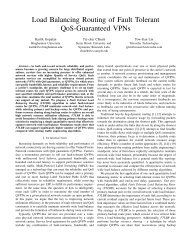
Fig. 2. Log-tail plot for the right tail of the sample distribution of NCC[s; r i ] for an unmatched case.
2.2 Error analysis
We make an assumption that, under hypothesis H 0 for a fixed scaling ratio r i , the values of the 2D normalized crosscorrelation
NCC[s; r i ] as a function of s are i.i.d. samples of a Gaussian random variable ζ ~ N (0, σ
() i
2
i
). This is a
plausible assumption due to the Central Limit Theorem and the fact that the two-dimensional signal K is wellmodeled
as realizations of white Gaussian noise. Since the model fit at the tails is important for proper error analysis,

we experimentally verified this assumption by providing in Fig. 2 the log-tail plot. It shows the probability
log 10 Pr{NCC > x} as a function of x (continuous line) and the same probability calculated from the sample
distribution of cross-correlations obtained experimentally for an incorrect scaling ratio for one selected test image. We
can see that the right tail is consistent with the Gaussian assumption.
Estimating the variance
a small central region N surrounding the peak
2
σ
i
of the Gaussian model using the sample variance
1
2
2
ˆ
i
=
NCC[; s r ]
mn−
| N | ss , ∉N
σ
∑
ˆi2
σ of NCC[s; r i ] over s after excluding
i
, (10)
() i
we now calculate the probability p i that ζ would attain the peak value NCC[s peak ; r peak ] or larger by chance. Using
(8) and (10),
2 2
∞
x
∞
x
= − −
1 2 2 ˆ
2 ˆ σ
1
i
2 ˆ σ
⎛σ
peak ⎞
i
i ∫
PCEpeak
ˆ
ˆ
ˆ
[ peak ; rpeak ] 2πσ
= ∫
i ˆ σ peak PCE
2πσ
= ⎜ ⎟
σ
NCC s
i
peak i
⎝ ⎠
p e dx e dx Q
= 1− ( 1−
p )
, (11)
where Q(x) = 1 – Φ(x) with Φ(x) denoting the cumulative distribution function of a normal variable N(0,1) and
PCE peak = PCE(r peak ). As explained in Section 2.1, during the search for the cropping vector s, we only need to search
in the range (7), which means that we are taking maximum over k i = (m – M/r i + 1)×(n – N/r i + 1) samples of ζ (i) . Thus,
the probability that the maximum value of ζ (i) would not exceed NCC[s peak ; r peak ] is
( 1−
)
. After R steps in the first
phase of the search
‡ and R' steps in the second phase, the probability of false alarm, P FA , (deciding H 1 while H 0 is
true) is
P
FA
R+
R'
∏
i=
1
ki
i
p i
. (12)
Since in our algorithm, we stop the search after the PCE reaches a certain threshold, we have r i ≤ r peak . Because
non-decreasing in i,
ˆ σ ˆ
peak
/ σ
i
≥ 1, and because Q(x) is decreasing, we have p i ≤ Q ( PCE peak )
k i
ˆi2
σ is
= p. Thus, because k i ≤
k
P ( p) FA
≤1− 1−
, (13)
mn, from (12) we obtain an upper bound on P FA
R−1 R'
∑ki
∑k'
i
i= 0 i=
1
where k = + is the maximal number of values of the parameters r and s over which the maximum of (6)
max
could be taken, k' i = (m – M/r' i + 1)×(n – N/r' i + 1).
The threshold for PCE, τ = τ (P FA , M, N, m, n), depends on the probability of false alarm P FA and the size of the search
space for the parameters, which is determined by the dimensions of PRNU and the dimensions of the image under
investigation. For example, for our tested Canon G2 camera with m = 1704 and n = 2272, image size M = 833,
N = 1070, P FA ≤ 10 –5 , R = 201 according to Step 2 and R' = 12 for Phase 2 of the search, k max = 88,836,025 and the
threshold for PCE is τ = 53.772.
3. EXPERIMENTAL RESULTS
Three types of experiments are presented in this section. The scaling only and cropping only experiments performed
on 5 different test images along with (and without) JPEG compression are in Section 3.1. Section 3.2 contains random
cropping and random scaling tests with JPEG compression on a single image. This test follows the most likely “real
life” scenario and reveals how each processing step affects camera identification. In Section 3.3, we discuss a special
case of cropping and scaling which occurs when digital zoom is engaged in the camera.
‡ Recall that the parameter R is the number of samples used in Phase 1 of the search for the scaling parameter.

3.1 Scaling only and cropping only
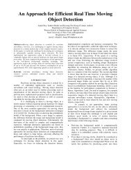
Fig. 3 shows five test images from Canon G2 with a 4 Mp CCD sensor. These images cover a wide range of
difficulties from the point of view of camera identification with the first one being the easiest because it contains large
flat and bright areas and the last one the most difficult due to its rich texture. 17 The camera fingerprint K was
estimated from 30 blue sky images in the TIFF format. It was also preprocessed using the column and row zeromeaning
17 to remove any residual patterns not unique to the sensor. This step is important because periodicities in
demosaicking errors would cause unwanted interference at certain translations and scaling factors, consequently
decreasing the PCE and increasing the false alarm rate. We found that this effect can be quite substantial.
We performed several different tests to first gain insight into how robust the camera ID algorithm is. In the Scaling
Only Test, we only subjected the test images to scaling with progressively smaller scaling parameter r and displayed
the results in Table 1 showing the PCE(r) for 0.3 ≤ r ≤ 0.9, with no lossy compression and with JPEG compression
with quality factors 90%, 75%, and 60%. The downsampling method was bicubic resampling. The upsampling used in
our search algorithm was the nearest neighbor algorithm. Here, we intentionally used a different resampling algorithm
because in reality we will not know the resampling algorithm and we want the tests to reflect real life conditions.
In the Cropping Only Test, all images were only subjected to cropping with an increasing amount of the cropped out
region. The cropped part was always the lower-right corner of the images. We note that while scaling by the ratio r
means that the image dimensions were scaled by the factor r, cropping by a factor r means that the size of the cropped
image is r times the original dimension. In particular, scaling and cropping by the same factor produces images with
the same number of pixels, r 2 × mn.
(1) (2) (3) (4) (5)
Fig. 3. Five test images from a 4 MP Canon G2 camera ordered by the richness of their texture (their difficulty to be identified).
The image identification in the Scaling Only Test (left half of Table 1) was successful for all 5 images and JPEG
compression factors when the scaling factor was not smaller than 0.5. It started failing when the scaling ratio was 0.4
or lower and the JPEG quality was 75% or lower. Image #5 was correctly identified at ratios 0.5 and above although
its content is difficult to suppress for the denoising filter. 17 The largest PCE that did not determine the correct
parameters [s peak ; r peak ] was 38.502 (image #1). On the other hand, the lowest PCE for which the parameters were
correctly determined was 35.463 (also for image #1). We encountered some cases when the maximum value of NCC
did occur for the correct cropping and scaling parameters but the identification algorithm failed because the PCE was
below the threshold set to achieve P FA ≤ 10 –5 .
Image cropping has a much smaller effect on image identification (the Cropping Only Test part of Table 1). We
correctly determined the exact position of the cropped image within the (unknown) original in all tested cases. The
PCE was consistently above 130 even when the images were cropped to the small size 0.3m × 0.3n and compressed
with JPEG quality factor 60.
3.2 Random cropping and random scaling simultaneously
This series of tests focused on the performance of the search method on image #2. The image underwent 50
simultaneous random cropping and scaling with both scaling and cropping ratios between 0.5 and 1 followed by JPEG
compression with the same quality factors as in the previous tests. We sorted the maximum PCE values found in each
search by the scaling ratio (since it has by far the biggest influence on the algorithm performance) and plotted the PCE
in Fig. 4. The threshold τ = 56.315 displayed in the figure corresponds to the worst scenario (largest search space) of
0.5 scaling and 0.5 cropping for false alarm rate below 10 –5 . In the test, we did not observe any missed detection for
the JPEG quality factor 90, 1 missed detection for JPEG quality factor 75 and scaling ratio close to 0.5, and 5 missed

detections for JPEG quality factor 60 when the scaling ratios were below 0.555. Even though these numbers will vary
significantly with the image content, they give us some insight into the robustness of the proposed method.
The last test was a large scale test intended to evaluate the real-life performance of the proposed methodology. The
database of 720 images contained snapshots spanning the period of four years. All images were taken at the full CCD
resolution and with a high JPEG quality setting. Each image was first subjected to a randomly-generated cropping up
to 50% in each dimension. The cropping position was also chosen randomly with uniform distribution within the
image. The cropped part was further resampled by a scaling ratio r∈[0.5, 1]. Finally, the image was compressed with
85% quality JPEG. The false alarm was set again to 10 –5 . Running our algorithm with r min = 0.5 on all images
processed this way, we encountered 2 missed detections (Fig. 5a), which occurred for more difficult (textured)
images. In all successful detections, the cropping and scaling parameters were detected with accuracy better than 2
pixels in either dimension.
To complement this test, 915 images from more than 100 different cameras were downloaded from the Internet in
native resolution, cropped to the 4 Mp size of Canon G2 and subjected to the same random cropping, scaling, and
JPEG compression as the 720 images before. No single false detection was encountered. All maximum values of PCE
were below the threshold with the overall maximum at 42.5.
Table 1. PCE in the Scaling Only Test followed by JPEG compression. The PCE is in italic when the scaling ratio was not
determined correctly. Values in parentheses are below the detection threshold τ (see the leftmost column) for P FA < 10 –5 .
r = 0.9
τ = 45.1
r = 0.8
τ = 48.3
r = 0.7
τ =P 50.4
r = 0.6
τ = 52.1
r = 0.5
τ = 53.5
r = 0.4
τ = 54.8
r = 0.3
τ = 55.9
Scaling Only Test
Cropping Only Test
Im. #1 Im. #2 Im. #3 Im. #4 Im. #5 Im. #1 Im. #2 Im. #3 Im. #4 Im. #5
TIFF 68003 32325 28570 20092 2964 14624 9157 7789 8961 3106
Q 90 28951 12834 11347 6971 1515 20905 11475 8223 7348 2637
Q 75 6131 3343 3436 2225 793 7192 4509 4668 3193 1480
Q 60 1778 1245 1291 1037 461 2751 2029 2227 1706 919
TIFF 72971 35086 30128 17494 2260 9282 8148 7764 8043 3058
Q 90 19041 8045 7080 4171 955 15287 8988 8251 6060 2329
Q 75 2980 1610 1736 1115 417 5698 2979 3977 2550 1226
Q 60 763 645 614 348 222 2216 1224 1916 1337 754
TIFF 41835 20058 17549 9674 910 6496 7986 7384 6030 2508
Q 90 8255 3642 3731 1938 410 11434 7887 9210 4533 2037
Q 75 1316 724 979 507 170 4565 2593 3807 2142 995
Q 60 328 318 406 203 124 1774 1155 1860 1139 622
TIFF 42192 18991 16902 8986 1001 4896 8249 6550 4353 1971
Q 90 4619 2060 2195 1311 422 7679 6328 8574 2918 1445
Q 75 625 399 476 214 117 2883 1951 3443 1255 682
Q 60 190 166 196 85 53 1166 709 1568 669 459
TIFF 24767 10719 9442 4781 487 4339 6592 5216 3006 1599
Q 90 1721 997 927 533 196 6314 3989 6996 2206 1265
Q 75 211 168 221 134 111 2622 1089 2799 1003 695
Q 60 144 56 70 (50) 58 1216 398 1322 574 464
TIFF 8083 3193 2897 1310 123 4008 4469 4163 1881 1086
Q 90 457 227 280 151 (52) 3730 2274 5178 1230 846
Q 75 72 (52) 72 (53) 31 1407 723 2113 570 453
Q 60 (35) (43) (43) 26 34 599 255 1006 311 324
TIFF 777 352 477 124 27 3518 1585 3030 916 837
Q 90 (46) (41) 60 38 30 2577 742 3414 657 609
Q 75 39 32 35 31 35 969 269 1378 300 259
Q 60 35 33 35 32 35 461 139 721 164 177

10 4
10 4
PCE
10 5 scaling factor
10 3
PCE
10 5 scaling factor
10 3
10 2
10 2
10 1
0.5 0.6 0.7 0.8 0.9 1
10 1
0.5 0.6 0.7 0.8 0.9 1
(a) JPEG quality factor 90
(b) JPEG quality factor 75
10 5 scaling factor
10 4
PCE
10 3
10 2
10 1
0.5 0.6 0.7 0.8 0.9 1
(c) JPEG quality factor 60
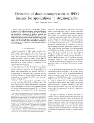
Fig. 4. PCE for image #2 after a series of random scaling and cropping followed by 90% quality JPEG compression.
10 5 scaling factor
10 2 scaling factor
10 4
th
PCE
10 3
PCE
10 2
th
10 1
0.5 0.6 0.7 0.8 0.9 1
0.5 0.6 0.7 0.8 0.9 1
(a) PCE as a function of the scaling ratio for 720 images
matching the camera.
(b) PCE for 915 images not matching the camera.
Fig. 5. “Real-life large scale test” for JPEG images subjected to random cropping and scaling and saved as 85% quality JPEG. The
lines mark the threshold for P FA ≤ 10 –5 (τ = 56.315). (a) 720 images from the camera, (b) 915 images from other cameras.

3.3 Digital zoom
While optical zoom does not desynchronize PRNU with the image noise residual (it is equivalent to a change of
scene), when a camera engages digital zoom, it introduces the following geometrical transformation: the middle part
of the image is cropped and up-sampled to the resolution determined by the camera settings. This is a special case of
our cropping and scaling scenario. Since the cropping may be a few pixels off the center, we need to search for the
scaling factor r as well as the shift vector s. The maximum digital zoom determines the upper bound on our search for
the scaling factor. For simplicity, we apply the same search for cropping as before although we could restrict
ourselves to a smaller search range around the image center.
Some cameras allow almost continuous digital zoom (e.g., Fuji E550) while other offer only several fixed values. This
is the case of Canon S2 that we tested. The camera display indicates zoom values “24×”, “30×”, “37×”, and “48×”,
which correspond to digital zoom scaling ratios 1/2, 1/2.5, 1/3.0833, and 1/4, considering the 12× camera optical
zoom. Our test revealed exact scaling ratios 1/2.025, 1/2.5313, 1/3.1154, and 1/4, corresponding to cropped sizes
1280×960, 1024×768, 832×624, and 648×486, respectively. Thus, in general for camera identification, we may wish
to check these digital zoom scaling values first before proceeding with the rest of the search if no match is found. We
note that none of the camera manuals for the two tested cameras (Fuji and Canon) contained any information about the
digital zoom. We only found out the details about their digital zooms using the PRNU! Thus, this is an interesting
example of using the PRNU as a template to recover processing history or reverse-engineer in-camera processing.
Table 2 shows the maximal PCE on 10 images taken with Canon S2 and Fuji E550, some of which were taken with
digital zoom. Both cameras were identified with very high confidence in all 10 cases. Images from Fuji camera
yielded smaller maximum PCEs, which suggests that (if the image content is dark or heavily textured) the
identification of Fuji E550 camera could be more difficult than Canon S2. The detected cropped dimensions (see
Table 2) are either precise or off only by a few pixels. This camera apparently has a much finer increment when
adjusting the digital zoom than Canon S2. Since the Fuji E550 user is not informed about the fact that the digital zoom
has been engaged, it may be quite tedious to find all possible scaling values in this case. The largest digital zoom the
camera offers for full resolution output size is 1.4. Fig. 6 shows images with detected cropped frame for the last two
Fuji camera images of the same scene.
The fact that we are able to obtain previous dimensions of the up-sampled images is an example of “reverse
engineering” for revealing image processing history. Such information is potentially useful in forensics sciences even
if the source camera is positively known beforehand.
Table 2. Detection of scaling and cropping for digitally zoomed images.
Canon S2
Fuji E550
Image
#
scaling
detected
max
PCE
cropped
dim
scaling
detected
max
PCE
cropped
dim
1 3.1154 1351 832×624 1.1530 358 2470×1853
2 2.5313 6020 1024×768 1.3434 238 2120×1590
3 2.0250 2792 1280×960 1.3940 102 2043×1532
4 2.0203 9250 1283×962 1.1837 310 2406×1805
5 2.5313 5929 1024×768 1.0234 576 2783×2087
6 3.1154 3509 832×624 1.0007 328 2846×2135
7 4.0062 2450 647×485 1.0000 314 2848×2136
8 4.0062 1265 647×485 1.0845 1022 2626×1970
9 4.0062 1620 649×487 1.1530 976 2470×1853
10 4.0062 1612 647×485 1.3428 378 2121×1591

Fig. 6. Cropping detected for Fuji E550 images #9 and #10.
4. CONCLUSIONS
In this paper, we present an extension of our previous work on camera identification from images using sensor pattern
noise. The proposed method is capable of identifying the camera after the image under investigation was
simultaneously cropped and scaled or when the image was taken with a digital zoom. The camera ID is formulated as
a two-channel detection problem. The detector is obtained using the generalized likelihood ratio test and has a form of
a cross-correlation maximized over the parameters of the geometrical transform. In fact, we recommend using crosscorrelation
and the PCE instead of the correlation as the detection statistics even for images that did not undergo any
geometrical processing because the cross-correlation surface enables more accurate error rate estimation. We report
the results for a wide range of scaling and cropping parameters and JPEG compression. The results indicate that
reliable camera ID is possible for images linearly scaled down by a factor of 0.5 or more or images with 90% or more
cropped away. The reliability depends on the image content and subsequent JPEG compression. We also demonstrate
that the sensor noise can be used as a template to reverse-engineer in-camera geometrical processing, such as
processing due to digital zoom. We acknowledge that the proposed method can be computationally expensive, namely
for large image dimensions. A hierarchical search that starts with a large step which is then decreased by ½ in each
round makes the search process about 4 times faster, however only if the match is positive.
ACKNOWLEGEMENT
The work on this paper was supported by the AFOSR grant number FA9550-06-1-0046. The U.S. Government is
authorized to reproduce and distribute reprints for Governmental purposes notwithstanding any copyright notation
thereon. The views and conclusions contained herein are those of the authors and should not be interpreted as
necessarily representing the official policies, either expressed or implied, of Air Force Research Laboratory, or the
U.S. Government.
REFERENCES
1. S. Bayram, H.T. Sencar, and N. Memon: “Source Camera Identification Based on CFA Interpolation.” Proc.
ICIP’05, Genoa, Italy, September 2005.
2. A. Swaminathan, M. Wu, and K.J.R. Liu: “Non-intrusive Forensic Analysis of Visual Sensors Using Output
Images.” Proc. IEEE Int. Conf. on Acoustics, Speech, and Signal Processing (ICASSP'06), May 2006.
3. A. Swaminathan, M. Wu, and K.J.R. Liu: “Image Authentication via Intrinsic Fingerprints.” Proc. SPIE,
Electronic Imaging, Security, Steganography, and Watermarking of Multimedia Contents IX, vol. 6505, January
29–February 1, San Jose, CA, pp. 1J–1K, 2007.
4. M. Kharrazi, H.T. Sencar, and N. Memon: “Blind Source Camera Identification,” Proc. ICIP’04, Singapore,
October 24–27, 2004.

5. K. Kurosawa, K. Kuroki, and N. Saitoh: “CCD Fingerprint Method – Identification of a Video Camera from
Videotaped Images.” Proc. ICIP’99, Kobe, Japan, pp. 537–540, October 1999.
6. Z. Geradts, J. Bijhold, M. Kieft, K. Kurosawa, K. Kuroki, and N. Saitoh: “Methods for Identification of Images
Acquired with Digital Cameras.” Proc. of SPIE, Enabling Technologies for Law Enforcement and Security, vol.
4232, pp. 505–512, February 2001.
7. J. Lukáš, J. Fridrich, and M. Goljan: “Digital Camera Identification from Sensor Pattern Noise.” IEEE
Transactions on Information Security and Forensics, vol. 1(2), pp. 205–214, June 2006.
8. H. Gou, A. Swaminathan, and M. Wu: “Robust Scanner Identification Based on Noise Features.” Proc. SPIE,
Electronic Imaging, Security, Steganography, and Watermarking of Multimedia Contents IX, vol. 6505, January
29–February 1, San Jose, CA, pp. 0S–0T, 2007.
9. N. Khanna, A.K. Mikkilineni, G.T.C Chiu, J.P. Allebach, and E.J. Delp III: “Forensic Classification of Imaging
Sensor Types.” Proc. SPIE, Electronic Imaging, Security, Steganography, and Watermarking of Multimedia
Contents IX, vol. 6505, January 29–February 1, San Jose, CA, pp. 0U–0V, 2007.
10. B. Sankur, O. Celiktutan, and I. Avcibas: “Blind Identification of Cell Phone Cameras.” Proc. SPIE, Electronic
Imaging, Security, Steganography, and Watermarking of Multimedia Contents IX, vol. 6505, January 29–
February 1, San Jose, CA, pp. 1H–1I, 2007.
11. T. Gloe, E. Franz, and A. Winkler: “Forensics for Flatbed Scanners.” Proc. SPIE, Electronic Imaging, Security,
Steganography, and Watermarking of Multimedia Contents IX, vol. 6505, January 29–February 1, San Jose, CA,
pp. 1I–1J, 2007.
12. N. Khanna, A.K. Mikkilineni, G.T.C. Chiu, J.P. Allebach, and E.J. Delp III: “Scanner Identification Using Sensor
Pattern Noise.” Proc. SPIE, Electronic Imaging, Security, Steganography, and Watermarking of Multimedia
Contents IX, vol. 6505, January 29–February 1, San Jose, CA, pp. 1K–1L, 2007.
13. C.W. Honsinger and S.J. Daly: “Method for Detecting Rotation and Magnification in Images,” United States
Patent 5,835,639, Kodak, 1998.
14. N. Nikolaidis and I. Pitas: “Circularly Symmetric Watermark Embedding in 2-D DFT Domain,” In: Proc. IEEE
Int. Conf. on Acoustics, Speech, and Signal Processing (ICASSP99), vol. 6, pp. 3469–3472, Phoenix, AZ, March
15–19, 1999.
15. J.J.K. Ó Ruanaidh and T. Pun: “Rotation, Scale and Translation Invariant Spread Spectrum Digital Image
Watermarking,” Signal Processing, vol. 66(5), pp. 303–317, May 1998.
16. A.C. Popescu and H. Farid: “Exposing Digital Forgeries by Detecting Traces of Resampling.” IEEE Transactions
on Signal Processing, vol. 53(2), pp. 758–767, 2005.
17. J. Fridrich, M. Chen, M. Goljan, and J. Lukáš: “Digital Imaging Sensor Identification (Further Study),” Proc.
SPIE, Electronic Imaging, Security, Steganography, and Watermarking of Multimedia Contents IX, vol. 6505,
San Jose, CA, January 28–February 2, pp. 0P–0Q, 2007.
18. M.K. Mihcak, I. Kozintsev, and K. Ramchandran: “Spatially Adaptive Statistical Modeling of Wavelet Image
Coefficients and its Application to Denoising,” Proc. IEEE Int. Conf. Acoustics, Speech, and Signal Processing,
Phoenix, Arizona, vol. 6, pp. 3253–3256, March 1999.
19. C.R. Holt: “Two-Channel Detectors for Arbitrary Linear Channel Distortion,” IEEE Trans. on Acoustics, Speech,
and Sig. Proc., vol. ASSP-35(3), pp. 267–273, March 1987.
20. B.V.K. Vijaya Kuma and L. Hassebrook: “Performance Measures for Correlation Filters,” Appl. Opt. 29, 2997–
3006, 1990.
21. S.M. Kay, Fundamentals of Statistical Signal Processing, Volume II, Detection theory, Prentice Hall, 1998.